


1. Introduction
Predicting the performance of a turbine array under realistic conditions still remains a challenge in our attempts to optimise the layout and operation of wind and tidal farms (Porté-Agel, Bastankhah & Shamsoddin Reference Porté-Agel, Bastankhah and Shamsoddin2020; Adcock et al. Reference Adcock, Draper, Willden and Vogel2021). This challenge encompasses both external factors such as interactions with the atmospheric boundary layer for wind farms, and internal factors such as turbulent wakes, which impact power extraction and fatigue loads (Sanderse, van der Pijl & Koren Reference Sanderse, van der Pijl and Koren2011). Due to the multi-scale nature of the problem it is practical to split the problem into two sub-problems: the external (farm-scale) and internal (turbine-scale) problems (Nishino & Dunstan Reference Nishino and Dunstan2020), and the internal sub-problem will be the focus of this study. The internal sub-problem is characterised by a range of turbine-scale features; these include local flow boundaries from neighbouring devices, the sea surface or seabed (for tidal). These boundaries can constrain the flow (Garrett & Cummins Reference Garrett and Cummins2007) or even produce additional fluid dynamical phenomena like surface gravity waves (for tidal) which can have a direct impact on the turbine-scale flow and wake development (Li et al. Reference Li, Ghia, Li, Fan and Shen2021). Note that, although gravity waves can impact wind farms as well (Ollier, Watson & Montavon Reference Ollier, Watson and Montavon2018) they are considered as part of the external sub-problem for wind (unless they are strong enough to have a direct impact on the local flow pattern around each turbine). The characteristics of the inflow are a key consideration for the internal sub-problem; the inflow profile, ambient turbulence and inflow direction can all have a large impact on the performance and wake of a turbine as well (Porté-Agel et al. Reference Porté-Agel, Bastankhah and Shamsoddin2020; Adcock et al. Reference Adcock, Draper, Willden and Vogel2021). Being able to accurately model these features is necessary as variations in local boundaries and wake mixing can have significant impacts on the performance of a turbine (Nishino & Willden Reference Nishino and Willden2013a). Analytical models of the internal sub-problem have traditionally been used to parameterise the impact of wind farms in meteorological models (Fitch et al. Reference Fitch, Olson, Lundquist, Dudhia, Gupta, Michalakes and Barstad2012; Abkar & Porté-Agel Reference Abkar and Porté-Agel2015) or tidal turbine arrays in ocean circulation models (Adcock et al. Reference Adcock, Draper, Houlsby, Borthwick and Serhadlíoğlu2013) and it is the extension to such analytical models of turbine arrays that this study will approach.
The most fundamental analytical model of turbines comes from the results of Lanchester, Betz and Joukowsky (van Kuik Reference van Kuik2007) which act as a foundational benchmark for the estimation of turbine performance. Their model, often referred to as the linear momentum actuator disc theory (LMADT), considers the conservation of linear momentum and energy in a streamtube which encases a turbine, and replaces the turbine with a porous actuator disc which exerts uniform streamwise resistance to a uniform inflow. Extensions to this model have been made to account for various flow types, from laterally confined inflow for a single turbine (Garrett & Cummins Reference Garrett and Cummins2007; Houlsby, Draper & Oldfield Reference Houlsby, Draper and Oldfield2008) and for a single row of turbines (Nishino & Willden Reference Nishino and Willden2012b, Reference Nishino and Willden2013b), to non-uniform inflow (Draper, Nishino & Adcock Reference Draper, Nishino and Adcock2014; Draper et al. Reference Draper, Nishino, Adcock and Taylor2016) and for multi-row systems (Juniper & Nishino Reference Juniper and Nishino2020; Ouro & Nishino Reference Ouro and Nishino2021). Although less accurate than numerical models based on the Navier–Stokes equations, their low computational cost makes them ideal for problems with large parameter spaces such as the optimisation of farm layout and operation control.
The interest in the flow confinement or ‘blockage’ effects encompasses two main applications, one being the performance of a turbine in a laboratory environment, and the other being for an array of turbines whose spanwise spacing may alter their performance due to ‘local’ blockage effects (Nishino & Willden Reference Nishino and Willden2012b; Nishino & Draper Reference Nishino and Draper2015). A number of blockage correction methods have been suggested over the years, and a recent experimental study by Ross & Polagye (Reference Ross and Polagye2020) compared a range of popular methods. The methods found to have the greatest agreement with the experiments were those of Houlsby et al. (Reference Houlsby, Draper and Oldfield2008) and Barnsley & Wellicome (Reference Barnsley and Wellicome1990). Note, the report of Barnsley & Wellicome (Reference Barnsley and Wellicome1990) does not appear to be publicly available; however, it was introduced by Bahaj et al. (Reference Bahaj, Molland, Chaplin and Batten2007) whose outline of the method echoes the approach of Garrett & Cummins (Reference Garrett and Cummins2007) placing a one-dimensional actuator disc in the middle of a rectangular channel (to consider additional streamtubes bypassing the disc as well as the ‘core’ streamtube passing through the disc). Barnsley & Wellicome's method solves a set of conservation equations with a given turbine thrust, with Houlsby et al.'s extension allowing for a deformable lateral boundary. The merit of closing the LMADT system with turbine thrust (instead of other physical quantities, such as the wake width) is that it can be measured accurately when utilising these models to correct for blockage in laboratory settings. Extensions to the thrust closure method are presented in this paper to address a wider range of flow features.
This paper firstly extends LMADT for a single turbine by analytically solving for a generalised number of bypass streamtubes, followed by a further extension for a generalised number of streamtubes passing through the turbine as well as in the bypass. These extensions aim to expand the current capabilities of LMADT to handle non-uniform inflow profiles along with variations in resistances across the turbine surface, allowing for a granular exploration of the impact of each of these components on the turbine performance in isolation. Although such an extension to consider non-uniform inflow has already been made by Draper et al. (Reference Draper, Nishino, Adcock and Taylor2016), in this paper we present a new formulation that leads to analytical solutions for any number of bypass streamtubes. This enables very fast calculations not only for a single turbine but also for a large number of turbines in a multi-row system.
The paper is structured such that in § 2 the theory and mathematics are presented along with a discussion of the assumptions made. In § 3 some example solutions for a single turbine are presented to explore the impact of averaging shear in the bypass and core flows, respectively, for select sheared inflow cases. In § 4 solutions for a selection of multi-row turbine arrays are presented and discussed. Discussion and conclusions of theoretical predictions, are presented in § 5.
2. Extended LMADT
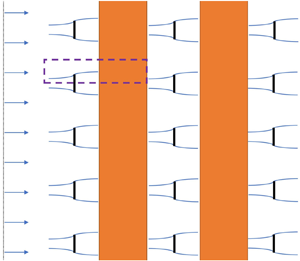
We consider many rows of spanwise equally spaced turbines as depicted in figure 1. The rows are considered to be infinitely wide (or sufficiently wide to ignore the spanwise end effect) and evenly spaced; therefore, we can exploit the symmetry in the system to only consider a local flow domain that is laterally bounded, as shown in figure 2. Note that the local domain here is constructed for the context of a turbine array, therefore  $y$ represents horizontal direction. However, $y$ can also be defined as the vertical direction when considering a single turbine in a channel with a rigid lid. The local flow domain is primarily defined by the blockage ratio $B$, where the cross-sectional area of the domain is $A/B$, with $A$ as the turbines swept area. Note that, for uniform inflow when $B \to 0$ the system limits to the Lanchester–Betz–Joukowsky case. As the LMADT only considers the local flow domain, it is assumed that the blockage ratio and inflow profile are both known.

Figure 1. Schematic of the flow past three rows of turbines arranged as perfectly aligned (left) and perfectly staggered (right) arrays, divided into inviscid (inv.) and viscous (visc.) flow zones. The rectangular region enclosed by the dashed line corresponds to the local flow domain depicted in figure 2.

Figure 2. Diagram of non-dimensionalised local flow domain with a single streamtube passing through the turbine.
The main assumptions employed in this analysis are that the flow is inviscid, incompressible and steady. The flow is also assumed to be symmetric about the centre of the turbine in two-dimensional (2-D) applications of the method and axisymmetric in 3-D applications. The actuator itself is modelled to apply a uniform force on the fluid; this will be discussed further in § 2.2.
For the 2-D case presented in this paper,  $A$ is our reference length defined as the length of the 1-D actuator strip and $u$ is our reference velocity (e.g. $u = 10$ m s $^{-1}$). The inflow profile is defined by $N+1$ segments with velocity $\phi _{i}u$ and cross-sectional area $R_{i}A$, where $0 < R_{i} \leq 1/B$ and $\phi _{i} > 0$. All velocity and area values are defined as a real positive scalar times $u$ and $A$, respectively, which act as dimensional parameters. At the downstream position the flow profile is defined by $N+2$ segments with velocity $\beta _{i}u$ and cross-sectional area $R_{\beta _{i}}A$, where $0 < R_{\beta _{i}} \leq 1/B$ and $\beta _{i} > 0$. The velocity through the turbine is $\alpha _{av}u$, with $\alpha _{av}>0$. We obtain an additional streamtube in the downstream as one of the upstream streamtubes is split by the turbine. For example, with one upstream streamtube (uniform inflow) we obtain two downstream streamtubes i.e. the bypass and the wake. Although $\phi _{0}$ is expressed explicitly in the formulations below all computations will be for normalised flow profiles such that $\phi _{0}=1$.
The problem can be split up into two cases that will be solved slightly differently. The first case is when the flow passing through the turbine has uniform velocity, as depicted in figure 2. The second case is when the flow velocity is non-uniform across the turbine, as depicted in figure 3.

Figure 3. Diagram of non-dimensionalised local flow domain with multiple streamtubes passing through the turbine.
2.1. Uniform flow through turbine
For uniform flow through a turbine Bernoulli's equation is first applied to the streamtubes which bypass the turbine. This gives
 \begin{equation} p_{1} + \tfrac{1}{2}\rho u^{2}\phi_{i}^{2} = p_{4} + \tfrac{1}{2}\rho u^{2}\beta_{i+1}^{2}, \end{equation}
for  $i\geq 0$, where $\rho$ is the fluid density, $p_{1}$ is the static pressure upstream of the turbine, $p_{2}$ and $p_{3}$ are the static pressures immediately upstream and downstream of the turbine, respectively, and $p_{4}$ is the static pressure downstream of the turbine. It is assumed for $p_{1}$ and $p_{4}$ that the pressure has equalised in the spanwise direction. This can be rewritten as
 \begin{equation} p_{1} - p_{4} = \tfrac{1}{2}\rho u^{2} (\beta_{i+1}^{2} - \phi_{i}^{2}). \end{equation}
As the pressure drop  $p_{1} - p_{4}$ is constant for all bypass streamtubes we can equate the right-hand side of (2.2) for two different bypass streamtubes (indexed $i$ and $j$) to obtain a relationship between the velocities
 \begin{equation} \beta_{j} = \sqrt{\beta_{i}^{2} - \phi_{i-1}^{2} + \phi_{j-1}^{2}}, \end{equation}
for  $i,j \geq$ 1. We can fix $i=1$ so only the downstream bypass flow speed for the streamtube that immediately bypasses the turbine ( $\beta _{1}$) is required to know all the other downstream bypass flow speeds ( $\beta _{2}$ to $\beta _{N+1}$). Furthermore, if the bypass flow speeds are known then all downstream areas of bypass streamtubes are known via the conservation of mass
 \begin{equation} R_{i}\phi_{i} = R_{\beta_{i+1}}\beta_{i+1}, \end{equation}
for  $i \geq 1$. Now considering the momentum balance for the entire domain between the upstream and downstream locations the thrust of the turbine is obtained as
 \begin{equation} \frac{T}{A} = \sum^{n}_{i=0} R_{i}\phi_{i}^{2}u^{2}\rho - \sum_{i=0}^{n+1} R_{\beta_{i}}\beta_{i}^{2}u^{2}\rho + \frac{1}{B}(p_{1} - p_{4}). \end{equation}
Using (2.2) with  $i=0$ to remove the pressure terms in the equation
 \begin{equation} \frac{T}{A} = \left( \sum^{n}_{i=0} R_{i}\phi_{i}^{2} - \sum_{i=0}^{n+1} R_{\beta_{i}}\beta_{i}^{2} + \frac{1}{2B} (\beta_{1}^{2} - \phi_{0}^{2})\right) u^{2}\rho. \end{equation}
Applying the Bernoulli equation upstream and downstream of the disc to obtain a relation between the pressure drop across the turbine and the velocity of the flow gives
 \begin{equation} (p_{1} - p_{2}) + (p_{3} - p_{4}) = \tfrac{1}{2} \rho u^{2} ((\alpha_{av}^{2} - \phi_{0}^{2}) + (\beta_{0}^{2} - \alpha_{av}^{2}) ). \end{equation}
Using the static equilibrium across the turbine the thrust is just the pressure drop across the turbine so from (2.7) we simplify to
 \begin{equation} \frac{T}{A} = p_{2} - p_{3} = \frac{1}{2}\rho u^{2} (\beta_{1}^{2} - \beta_{0}^{2} ). \end{equation}
We will set the flow speed  $u$, turbine area $A$ and density $\rho$ equal to 1 for simplicity in the rest of the calculation. Now equating (2.6) and (2.8) gives
 \begin{equation} \frac{1}{2}(\beta_{1}^{2} - \beta_{0}^{2}) = \sum^{n}_{i=0} R_{i}\phi_{i}^{2} - \sum_{i=0}^{n+1} R_{\beta_{i}}\beta_{i}^{2} + \frac{1}{2B} (\beta_{1}^{2} - \phi_{0}^{2}). \end{equation}
From the conservation of mass applied to the streamtube which encompasses the turbine, the following expression is obtained:
 \begin{align} R_{0}\phi_{0} &= R_{\beta_{1}}\beta_{1} + R_{\beta_{0}}\beta_{0} \nonumber\\ &= \beta_{1}\left(\frac{1}{B} - \sum^{n+1}_{i=2} R_{\beta_{i}} - R_{\beta_{0}}\right) + \alpha_{av} \nonumber\\ &= \beta_{1}\left(\frac{1}{B} - \sum^{n+1}_{i=2} R_{\beta_{i}} - \frac{\alpha_{av}}{\beta_{0}}\right) + \alpha_{av}. \end{align}
This can be rewritten in terms of  $\alpha _{av}$ as
 \begin{equation} \alpha_{av} = \frac{\beta_{0} \left( R_{0}\phi_{0} - \beta_{1} \displaystyle\left(\frac{1}{B} -\sum^{n+1}_{i=2} R_{\beta_{i}}\right) \right)}{(\beta_{0}-\beta_{1})}. \end{equation}
Re-arranging (2.9) can give
 \begin{align} \beta_{0}^{2} + 2\left( R_{0}\phi_{0}^{2} - R_{\beta_{0}}\beta_{0}^{2} - R_{\beta_{1}}\beta_{1}^{2} + \sum^{n}_{i=1} R_{i}\phi_{i} (\phi_{i} - \beta_{i+1})\right) + \frac{1}{B}(\beta_{1}^{2}-\phi_{0}^{2}) - \beta_{1}^{2}= 0. \end{align}
By the conservation of mass of the core flow  $R_{\beta _{0}}\beta _{0} = \alpha _{av}$, and along with $R_{\beta _{1}}\beta _{1} = R_{0}\phi _{0} - \alpha _{av}$ equation (2.12) can be rewritten as:
 \begin{align} & \beta_{0}^{2} - 2\alpha_{av}\beta_{0} +2\beta_{1}\alpha_{av} + 2\left( R_{0}\phi_{0}(\phi_{0} -\beta_{1}) + \sum^{n}_{i=1} R_{i}\phi_{i} (\phi_{i} - \beta_{i+1})\right) \nonumber\\ &\quad + \frac{1}{B}(\beta_{1}^{2}-\phi_{0}^{2}) - \beta_{1}^{2}= 0. \end{align}
Let
 \begin{equation} C_{1} = 2\left( R_{0}\phi_{0}(\phi_{0} -\beta_{1}) + \sum^{n}_{i=1} R_{i}\phi_{i} (\phi_{i} - \beta_{i+1})\right) + \frac{1}{B}(\beta_{1}^{2}-\phi_{0}^{2}) - \beta_{1}^{2}, \end{equation}
and
 \begin{equation} C_{2} = \left( R_{0}\phi_{0} - \beta_{1}\left(\frac{1}{B} -\sum^{n+1}_{i=2} R_{\beta_{i}}\right) \right). \end{equation}
Now substitute (2.11) in for  $\alpha _{av}$ to obtain
 \begin{equation} \beta_{0}^{3} - (2C_{2} +\beta_{1})\beta_{0}^{2} + (2C_{2}\beta_{1} + C_{1})\beta_{0} - C_{1}\beta_{1}=0, \end{equation}
which is a cubic equation of  $\beta _{0}$ that can be solved analytically if we fix $\beta _{1}$, as $C_{1}$ and $C_{2}$ are functions of known terms and downstream bypass flow terms which can be obtained from $\beta _{1}$ using (2.3) and (2.4). The power generated by the turbine assuming no internal losses is
 \begin{equation} P=T\alpha_{av}u = \alpha_{av}(\beta_{1}^{2} - \beta_{0}^{2}) \left(\tfrac{1}{2}\rho A u^{3}\right)= C_{P} \left(\tfrac{1}{2}\rho A u^{3}\right), \end{equation}
reintroducing the area, density and velocity terms for clarity. Note that the power coefficient of the turbine,  $C_{P}$, is a function of $\alpha _{av}$ (2.11), $\beta _{1}$ and $\beta _{0}$, where only one of these needs to be given to set the operating condition of the turbine and thus solve the problem. In LMADT it is common to introduce a disc resistance (or local thrust) coefficient $k$ to describe the operating condition of the turbine such that
 \begin{equation} T = \tfrac{1}{2}k\rho A (\alpha_{av}u)^{2}, \end{equation}
therefore  $k= (\beta _{1}^{2} - \beta _{0}^{2})/\alpha _{av}^{2}$, by equating (2.17) and (2.18). Hence, the value of $C_{P}$ can be calculated analytically for a given set of $k$,
$k$,  $B$ and a given inflow profile ( $R_{i}$ and $\phi _{i}$).
The generalised approach means we are not constrained by the number of bypass streamtubes calculated. This removes, for example, the need to reduce the number of streamtubes through mixing assumptions used in previous multi-row studies which could result in substantial differences in the predicted power (Juniper & Nishino Reference Juniper and Nishino2020).
2.2. Non-uniform flow through turbine
When considering non-uniform flow through a turbine the calculations are much the same as the uniform case presented in § 2.1. A choice is required, however, on how to model the actuator disc. For uniform flow through a turbine there is little decision to be made as all methods considered for the non-uniform case produce equal results. The first method, is to keep the resistance,  $k$, uniform across the turbine. The second is to define the velocity profile across the turbine. The final approach considered is to maintain thrust, and therefore ${\rm \Delta} p$, to be uniform across the turbine.
The first method is often used as it gives a more accurate representation of an ideal porous disc which is often used as a representation of a turbine in experimental work (e.g. Myers & Bahaj Reference Myers and Bahaj2012) and in computational studies (e.g. Nishino & Draper Reference Nishino and Draper2015).
Draper et al. (Reference Draper, Nishino, Adcock and Taylor2016) obtain a uniform local resistance coefficient  $k$ for an unblocked turbine; however, this is a consequence of defining the flow velocity across the turbine. For the blocked case they restrict their attention to the case where $\alpha _{i}/\phi _{i}$ is constant across the disc, i.e. the velocity profile through the turbine is self-similar upstream. Here, $\alpha _{i}$ is a scalar such that $\alpha _{i}u$ is the velocity of the $i$th streamtube that passes through the turbine. Draper et al. (Reference Draper, Nishino, Adcock and Taylor2016) note that in flow that is not highly sheared or highly blocked the above method results in a near uniform resistance.
Chamorro & Arndt (Reference Chamorro and Arndt2013) adopted the third method, uniform thrust, constructing a correction factor to the Lanchester–Betz–Joukowsky limit for a turbine in a neutrally stratified atmospheric boundary layer. This method will be adopted in our calculation for non-uniform flow through a turbine. In support of this approach Revaz & Porté-Agel (Reference Revaz and Porté-Agel2021) found through large-eddy simulation that a model which computes non-uniform force distributions over the turbine and a model which assumes uniform forces over the turbine can both make accurate predictions for the flow in the far wake and power of the turbine. An exploration of the impact of non-uniform force for LMADT is presented in Appendix A.2.
For non-uniform flow through the turbine we start off as before by applying Bernoulli's equation to streamtubes that bypass the turbine
 \begin{equation} p_{1}-p_{4} = \tfrac{1}{2}\rho u^{2} (\beta_{i+1}^{2} - \phi_{i}^{2}), \end{equation}
which can be equated to obtain a relationship between all the bypass flow velocities
 \begin{equation} \beta_{i+1} = \sqrt{\beta_{j+1}^{2} + \phi_{i}^{2} - \phi_{j}^{2}}, \end{equation}
for  $i,j \geq M$, where $M$ is the index of the streamtube that is split by the turbine, as depicted in figure 3. Applying Bernoulli's equation to streamtubes that pass through the turbine gives us
 \begin{equation} p_{2}-p_{3} = {\rm \Delta} p = \tfrac{1}{2}\rho u^{2} (\phi_{a}^{2} - \beta_{a}^{2} - \phi_{M}^{2} + \beta_{M+1}^{2}), \end{equation}
and, as  ${\rm \Delta} p$ is held constant,
 \begin{equation} \beta_{a} = \sqrt{\beta_{b}^{2} + \phi_{a}^{2} - \phi_{b}^{2}}, \end{equation}
for  $a,b \leq M$. So all streamtube velocities are related once one downstream velocity in the bypass and one downstream velocity in the core flow are known. Likewise the conservation of momentum is defined as
 \begin{align} 0 &= (\beta_{M}^{2} - \beta_{M+1}^{2}) + \frac{1}{B}(\beta_{M+1}^{2} - \phi_{M}^{2}) + 2\left(\sum_{i=0}^{M-1} R_{i}\phi_{i}(\phi_{i} - \beta_{i}) \vphantom{\sum_{i=M+1}^{n}}\right. \nonumber\\ &\quad \left. + \sum_{i=M+1}^{n} R_{i}\phi_{i}(\phi_{i} - \beta_{i+1}) + R'\phi_{M}(\phi_{M}-\beta_{M}) + R^{*}\phi_{M}(\phi_{M}-\beta_{M+1}) \right), \end{align}
where  $R_{M} = R' + R^{*}$ with $R'$ as the upstream area of the streamtube which passes through the turbine and $R^{*}$ being the upstream area of the streamtube which directly bypasses the turbine.
The power  $P$ is calculated as
 \begin{equation} P = \sum_{i=0}^{M}R_{\alpha_{i}}A\alpha_{i}u {\rm \Delta} p, \end{equation}
where  $R_{\alpha _{i}}A$ is the size of the $i$th streamtube at the turbine plane; however, $R_{\alpha _{i}}$ is not calculated in this analysis. Therefore, this is rewritten using the conservation of mass to obtain an equivalent expression based on known upstream values
 \begin{equation} P = Au{\rm \Delta} p \left(R'\phi_{M} + \sum_{i=0}^{M-1} R_{i}\phi_{i}\right). \end{equation}
We define the power coefficient as
 \begin{equation} C_{P} = \frac{P}{\dfrac{1}{2}\rho A \overline{u^{3}}} = \frac{P}{\dfrac{1}{2}\rho A} \frac{R'+\displaystyle\sum^{M-1}_{i=0}R_{i} }{u^{3} \left(R'\phi_{M}^{3} +\displaystyle\sum_{i=0}^{M-1} R_{i}\phi_{i}^{3}\right)}, \end{equation}
which is the power normalised using the cube of the upstream velocity of the flow that passes through the turbine,  $\overline {u^{3}}$. To solve this system, we need to know what portion of upstream flow passes through the turbine, allowing $M$ to be determined. For this reason $\alpha _{av}$, the average velocity through the turbine, is used as the input parameter, thus allowing $M$ to be determined by conservation of mass. After $\alpha _{av}$ is selected a range of $\beta _{M+1}$ and $\beta _{M}$ values are iterated over to find the relevant root. The combinations of all $\beta _{M+1}$ and $\beta _{M}$ values do not need to be checked. It is possible to solve the system by first solving a corresponding uniform case and then solving for the non-uniform core flow; this is done by averaging the flow through the turbine such that it is uniform and has the same mass as the non-uniform and correcting (2.18) to account for the additional momentum in the non-uniform case. This fixes $\beta _{M+1}$, which will be equal between the uniform and non-uniform cases. Then $\beta _{M}$ can be found using (2.21) and the conservation of mass in the core flow.
3. Single-row results
Now we present some example solutions of the extended LMADT for a single turbine or a single row of turbines. It is worth noting that common wake models such as Jensen (Reference Jensen1983) assume a ‘top-hat’ profile for turbine wakes with locally uniform velocity instead of the more realistic sheared profile. The main aim of this section is therefore to investigate the physical implications of such a simplification of the inflow profile on the performance of a turbine in a laterally bounded domain.
3.1. Effective blockage with sheared bypass flow
A study into the impact of non-uniform inflow on the power of a turbine has been conducted by Draper et al. (Reference Draper, Nishino and Adcock2014), in which they found that a faster (or slower) bypass flow, compared with the core flow, could increase (or decrease) the power extracted by a turbine. This was explained by a change in the ‘effective blockage’ of the turbine, i.e. the faster (or slower) bypass flow inhibits (or enhances) the expansion of the core flow for a given geometrical blockage.
The effective blockage of a turbine is the blockage ratio required to attain the same  $C_{P\,{{max}}}$ with a uniform inflow. Since $C_{P\,{{max}}}$ for the case with uniform inflow is known to be $16/(27(1-B)^{2})$ (Garrett & Cummins Reference Garrett and Cummins2007; Dehtyriov et al. Reference Dehtyriov, Schnabl, Vogel, Draper, Adcock and Willden2021), the effective blockage, $B_{eff}$, is calculated as
 \begin{equation} B_{eff} = 1 - \left(\frac{16}{27 C_{P\,{{max}}}} \right)^{{1}/{2}}. \end{equation}
 The results of this work by Draper et al. (Reference Draper, Nishino and Adcock2014) was limited by the top-hat inflow profile shape, as shown in figure 4(a), where  $r$ is the width of the core flow and $\phi u$ is the velocity of the bypass. It was unclear whether this top-hat inflow profile would accurately predict the flow induced blockage of sheared bypass flows. Draper et al. (Reference Draper, Nishino, Adcock and Taylor2016) investigated the effective blockage of a turbine experiencing a variety of sheared inflow profiles. However, their study considers shear flow across the whole domain so cannot fully clarify the impact of a sheared bypass compared with a uniform bypass on the power extraction of turbine.

Figure 4. Contours of effective blockage ratio,  $B_{eff}$, for (a,c) uniform bypass and (b,d) sheared bypass cases, for fixed geometric blockage ratios (a,b) $B=0.2$ and (c,d) $B=0.1$.
In this study a comparison of the effective blockage was conducted between the cases with a top-hat inflow profile and a flow profile with a uniform core and linearly sheared bypass flow, as shown in 4(b). For the sheared case the upstream number of streamtubes is set at 201, which was found to be sufficient to accurately obtain the values of  $C_{P\,{{max}}}$ and thus $B_{eff}$ (see figure 5). To make a fair comparison, the mass flux in the bypass is held constant between the uniform bypass and linearly sheared cases.

Figure 5. Value of  $C_{P\,{{max}}}$ plotted against number of bypass streamtubes $N$ for $B=0.2$, $r=1$ and six different $\phi$ values.
The effective blockage for various bypass speeds and bypass sizes is plotted in figure 4 for two different blockage ratios  $B=0.2$ and $0.1$. When $\phi = 1$ we obtain the Garrett & Cummins (Reference Garrett and Cummins2007) result for a blocked turbine experiencing uniform inflow. Across all bypass sizes and bypass speeds the uniform bypass scenarios predict a higher effective blockage than the sheared bypass flow cases. This is more prominent for the lower blockage case of $B=0.1$. The over-prediction by the uniform bypass case occurs as for a given background pressure gradient the uniform bypass case restricts the expansion of the core flow more than the sheared bypass case; thus less flow is diverted around the turbine. The additional constraint from the uniform bypass flow can be illustrated from the increased effective blockage ratio $B_{eff}$ in the uniform case compared with the sheared bypass in figure 4.
The reduction in  $B_{eff}$ across all $r$ and $\phi$ values for the linear shear, in comparison with the uniform bypass, implies that the performance of a turbine placed in another turbine's wake may be consistently over-predicted when the upstream bypass flow is modelled as uniform instead of sheared. This result has implication for the use and benchmarking of wake models which maintain a top-hat flow profile in downstream like that of Jensen (Reference Jensen1983) and Frandsen et al. (Reference Frandsen, Barthelmie, Pryor, Rathmann, Larsen, Højstrup and Thøgersen2006) when applied to the analysis of multi-row turbine arrays. These top hat wake models are popular analytical models for turbine wakes which are still used today for turbine array optimisation (e.g. Duc et al. Reference Duc, Coupiac, Girard, Giebel and Göçmen2019).
3.2. Effective blockage with sheared core flow
In the previous section the impact of resolution/flow averaging on the power coefficient of a laterally bounded turbine with a sheared bypass flow was identified. In this section the impact of flow averaging for a shear flow passing through a turbine will be explored by comparing two flow profiles, sheared core and uniform core.
The base inflow profile which spans the domain will be a linear shear profile of the form
 \begin{equation} \phi = (1-\delta) + (2\delta)\frac{y}{A}, \end{equation}
where  $y/A$ is the non-dimensional spanwise distance from the centre of the turbine and $\delta$ is a parameter to define the significance of the shear. The portion of the flow which passes through the turbine will either be kept as a shear profile or be averaged to become a uniform flow profile, as illustrated in figure 6(b). All results presented below are for geometric blockage ratios of $B=0.1$ and $B=0.2$. The spanwise resolution of the flow was defined by fixing the number of upstream streamtubes which pass through the turbine at 20, as it was found to be adequate to ensure convergence with a difference of less than 0.2 % compared with calculating 500 streamtubes through the turbine.

Figure 6. Difference in the effective blockage between the uniform flow through a turbine and the shear flow through a turbine, for fixed geometric blockage ratios (a)  $B = 0.1$ and (b) $B=0.2$.
The effective blockage is plotted against  $\delta$ in figure 6 for the case of sheared flow through the turbine and uniform flow through the turbine. Across all $\delta$ values the uniform core flow case exaggerates the impact of the faster (if $\delta$ is positive) or slower (if $\delta$ is negative) bypass flow on the effective blockage. For negative $\delta$ values where the slower bypass leads to effective blockages lower than the geometric blockage ratio, a uniform core flow will under-predict the power extracted when compared with the sheared core flow case. Conversely, for positive $\delta$ values where the faster bypass increases the effective blockage ratio, a uniform core flow will over-predict the power extracted when compared with the sheared core flow case.
The theoretical approach detailed in § 2.2 only needs to consider which streamtube passes through the turbine and which enters the bypass. Hence, the spanwise position of each streamtube within the core or bypass flow does not impact the results, as long as the streamtube with velocity  $\phi _{M}u$ is still split by the turbine. Therefore, although simple linear shears were considered for this analysis, the trends observed here can be expected in cases with more complicated flow profiles as long as the above condition is satisfied.
4. Multi-row results
The previous section explored the impact of non-uniform inflow on a single turbine in a laterally bounded domain. This section conducts an analysis of multi-row turbine arrays modelled with the inviscid–viscous approach.
4.1. Local and global power coefficients
A distinction is made here between what we define as the ‘internal’ and ‘external’ performance of a multi-row array. To demonstrate this distinction in a simple manner, we first consider a special case of multi-row arrays where the streamwise distance between each row is large enough for the wake of each turbine to be fully recovered. This special case has been studied in a tidal turbine array context by Vennell (Reference Vennell2010) who combined the LMADT of Garrett & Cummins (Reference Garrett and Cummins2007) with an analytical tidal channel model (Garrett & Cummins Reference Garrett and Cummins2005). We present an equivalent special case in the wind turbine array context by combining results from the LMADT (with uniform inflow for each turbine) and an analytical ‘external’ model derived from the two-scale momentum theory for large wind farms (Nishino & Dunstan Reference Nishino and Dunstan2020).
We define the array-average ‘local’ or ‘internal’ power coefficient as
 \begin{equation} C_{P}^{*} = \frac{\displaystyle\sum^{n}_{i=1} P_{i}}{\dfrac{1}{2}\rho u_{av}^{3} n A}, \end{equation}
where  $P_{i}$ is the power at the $i$th turbine and $n$ the number of turbines in the array. This represents the total power of turbines for a given (fixed) mass flux through the local flow domain. Here, we assume that the average velocity, $u_{av}$, corresponds to the ‘farm-layer average’ velocity, $U_{F}$, in the two-scale momentum theory (as the inflow profile is uniform for all turbines and thus we cannot define the farm layer in this simple example). By keeping the mass flux constant through the local flow domain we restrict our attention to the ‘internal’ performance of the array, which can increase due to local blockage effects. This is in contrast to ‘global’ performance which can be impacted by wind-farm blockage effects (Bleeg et al. Reference Bleeg, Purcell, Ruisi and Traiger2018; Kirby, Nishino & Dunstan Reference Kirby, Nishino and Dunstan2022) reducing the power of a wind farm as the mass flux through the whole array decreases. Alongside the local power coefficient $C_{P}^{*}$, we also define the array-averaged ‘global’ power coefficient as
 \begin{equation} C_{P}^{G} = \frac{\displaystyle\sum^{n}_{i=1} P_{i}}{\dfrac{1}{2}\rho U_{0}^{3} n A}, \end{equation}
where  $U_{0}$ is undisturbed or ‘natural’ wind speed observed when the whole wind farm does not exist. Therefore, $C_{P}^{G}$ is a measure of the ‘overall’ efficiency of the farm, represented by the ratio of power extracted by the turbines and the power of the undisturbed flow through the total turbine swept area. Here, $C_{P}^{G} = \beta ^{3} C_{P}^{*}$, where $\beta = u_{av}/U_{0}$. To illustrate the impact of local blockage on $C_{P}^{G}$ and $C_{P}^{*}$, we compare how theses power coefficients change as we vary the lateral turbine spacing in a multi-row turbine array.
We calculate  $C_{P}^{*}$ directly from LMADT, whereas $C_{P}^{G}$ is estimated by combining LMADT results with the two-scale momentum theory of Nishino & Dunstan (Reference Nishino and Dunstan2020). To estimate the unknown velocity ratio, $u_{av}/U_{0}$, from the theory, we consider that there are multiple rows of turbines placed equidistantly with a large streamwise spacing of $20D$, where $D$ is the turbine diameter, and assume that this distance is large enough for each turbine wake to be fully recovered (see e.g. Sedaghatizadeh et al. Reference Sedaghatizadeh, Arjomandi, Kelso, Cazzolato and Ghayesh2019). This allows us to calculate the array density $\lambda$ (which is the ratio of the total turbine swept area to the farm area) as a function of the lateral turbine spacing $L$, i.e. $\lambda = {\rm \pi}D/80L$. We further assume a simple relationship between $B$ and $L$ as $B = {\rm \pi}D/20L$ for convenience, meaning that the height of the local flow domain (which may be defined when there is a strong capping layer acting like a rigid lid) is $5D$. This means that we assume $\lambda = 0.25B$ in the following analysis.
To solve the two-scale coupled problem, we also need to calculate from LMADT the array-averaged ‘local’ or ‘internal’ thrust coefficient, defined as
 \begin{equation} C_{T}^{*} = \frac{\displaystyle\sum^{n}_{i=1} T_{i}}{\dfrac{1}{2}\rho u_{av}^{2} n A}, \end{equation}
where  $T_{i}$ is the thrust at the $i$th turbine. The two-scale coupled momentum balance equation from Nishino & Dunstan (Reference Nishino and Dunstan2020) is
 \begin{equation} C_{T}^{*} \frac{\lambda}{C_{f0}}\beta^{2} + \beta^{\gamma} = 1 + \zeta(1-\beta), \end{equation}
where the momentum availability factor (right-hand side) has been approximated using a linear wind extractability model (Patel, Dunstan & Nishino Reference Patel, Dunstan and Nishino2021). Here, we also set the natural bottom friction coefficient as  $C_{f0} = 0.002$ to be typical of an offshore wind-farm scenario. We set the bottom friction exponent as $\gamma = 2$, which is a reasonable value and allows for the momentum equation (4.4) to be solved analytically. Therefore, $\beta$ is reduced to a function of an external (mesoscale) flow parameter $\zeta$. Here, $\zeta$ is the momentum response parameter for the atmosphere, which represents the ability of the atmosphere to sustain wind speed against the resistance caused by the wind farm, i.e. the extractability of wind. Typical values of which are expected to be between 5 and 25 for a realistic large offshore wind farm (Patel et al. Reference Patel, Dunstan and Nishino2021).
Figure 7 shows the values of  $C_{P}^{*}$ and $C_{P}^{G}$ (for three different atmospheric response strengths, $\zeta$ = 5, 15 and 25) across a range of turbine resistance coefficients and blockage ratios. In each plot the red line shows the optimal resistance coefficient, $k_{opt}$, which is defined as the value of $k$ at which the maximum power coefficient is achieved at each blockage ratio $B$. If $k$ is fixed the local power coefficient $C_{P}^{*}$ always increases with $B$, whereas the global power coefficient $C_{P}^{G}$ tends to decrease at different rates depending on $\zeta$. Importantly, the value of $k_{opt}$ for $C_{P}^{*}$ increases rapidly with $B$ (from 2 at $B$ = 0 to 5.4 at $B$ = 0.2) but $k_{opt}$ for $C_{P}^{G}$ tends to decrease, especially when $\zeta$ is small.

Figure 7. Contour plots of (a)  $C_{P}^{*}$ and (b–d) $C_{P}^{G}$ of a multi-row turbine array without wake interactions between rows, for (b) $\zeta = 5$, (c) $\zeta = 15$ and (d) $\zeta = 25$ for various blockage ratios ( $B$) and resistance coefficients ( $k$). Optimal resistance $k_{opt}$ is shown by a red line.
Figure 8 shows the maximum  $C_{P}^{*}$ and corresponding $C_{P}^{G}$ values obtained with $k=k_{opt}^{*}$ at each blockage ratio $B$, where $k_{opt}^{*}$ is the $k_{opt}$ value for $C_{P}^{*}$. Increasing $B$ (or decreasing the lateral turbine spacing $L$) causes $C_{P\,{{max}}}^{*}$ to increase, as observed in figure 7(a), however, $C_{P}^{G}$ at $k=k_{opt}^{*}$ decreases monotonically for all values of $\zeta$ between 5 and 25 (as the increase in $C_{P}^{*}$ is not large enough to compensate for the decrease in $\beta ^3$). Note that $B = {\rm \pi}D/20L$ has been assumed in this example and hence $B = 0.157$ corresponds to $L/D =1$, meaning that blockage ratios of higher than 0.157 are unphysical in this example (unless we allow for variable turbine hub heights in each row).

Figure 8. Maximum local power coefficient and corresponding global power coefficients of a multi-row turbine array without wake interactions between rows, plotted against the blockage ratio ( $B$) for a range of momentum response parameters ( $\zeta$) (with the assumption that $\lambda = 0.25B$, $C_{f0} = 0.002$ and $\gamma = 2$).
Note that, while a streamwise spacing of  $20D$ was selected for the above analysis, larger spacing may be required for each turbine wake to be fully recovered in a real wind farm depending on the turbulence intensity. However, the trends in the relationship between the local and global power coefficients observed in this exploration remain consistent across choices of spacing.
In the following sections we consider the more general case where the streamwise distance between rows is not large enough for the wake to be fully recovered. To model this we use an inviscid–viscous approach, outlined in the next sub-section, but for simplicity no longer consider the external momentum balance, therefore we only focus on the ‘internal’ performance of the array represented by  $C_{P}^{*}$.
4.2. Inviscid–viscous approach
For the following multi-row analysis we utilise the inviscid–viscous approach as described in Ouro & Nishino (Reference Ouro and Nishino2021). As illustrated earlier in figure 1, this approach treats the region around the turbine as an inviscid flow region which is modelled with LMADT, followed by a viscous mixing zone downstream which is modelled separately. This approach is in line with the results of West & Lele (Reference West and Lele2020) who, in a large-eddy simulation study of flow around an actuator disc, showed that inviscid flow processes dominate around the turbine and viscous processes dominate further downstream. We adopt the same simplification in this analysis as in Ouro & Nishino (Reference Ouro and Nishino2021) that mixing takes place uniformly across the viscous mixing zone and will be defined by a single parameter  $0\leq m\leq 1$ such that $u_{out} = m u_{av} + (1-m) u_{in}$, where $u_{in}$ is a streamtubes velocity entering the viscous mixing zone, $u_{av}$ is the average velocity across the whole domain and $u_{out}$ is the velocity as it exits the viscous mixing zone. For example when $m=1$ the whole flow becomes uniform and when $m=0$ no mixing occurs.
4.3. Instant mixing assumption and its validation
Previous utilisations of the inviscid–viscous approach for an infinitely large array of turbines (Nishino & Draper Reference Nishino and Draper2019; Ouro & Nishino Reference Ouro and Nishino2021) only calculate a fixed number of bypass streamtubes. As the number of streamtubes in the system increases at each turbine row (meaning that an infinite number of streamtubes would be required to model an infinitely large array), an assumption was made to keep the number of bypass streamtubes fixed. The assumption is that the bypass flow in the streamtube adjacent to the turbine (the streamtube with velocity  $\beta _{1}$ in figure 2) is always fully mixed in the viscous mixing zone (regardless of the value of the mixing parameter $m$) with the bypass flow in the streamtube immediately outside (the streamtube with the velocity $\beta _{2}$). In the case with uniform flow through the turbine the streamtubes with velocity $\beta _{1}u$ and $\beta _{2}u$ are mixed to a single streamtube with the new velocity coefficient
 \begin{equation} \beta' = \frac{R_{\beta_{1}}\beta_{1}+R_{\beta_{2}}\beta_{2}}{R_{\beta_{1}}+R_{\beta_{2}}}, \end{equation}
therefore the number of bypass streamtubes remains constant in the upstream and downstream.
The extended LMADT for a generalised number of bypass streamtubes outlined in § 2 allows for the impact of this instant mixing assumption to be accurately quantified. For this investigation both an aligned and a staggered turbine arrangement are considered with the first turbine row experiencing a fully uniform inflow. For a fixed blockage ratio and mixing rate,  $B=0.2$ and $m=0.6$, the array-averaged power coefficient $C_{P}^{*}$ of four rows of turbines is plotted in figure 9 against resistance coefficient $k$ for three different levels of instant mixing. Firstly, the ‘one bypass’ case is for instant mixing such that there are only up to two upstream streamtubes (i.e. the number of streamtubes increases from two to three in the inviscid zone but decreases from three to two due to the instant mixing between the two bypass flows in the viscous zone), the ‘two bypass’ case allows for three upstream streamtubes, and the ‘three bypass’ case allows for four upstream streamtubes. The three bypass case is therefore the case where no instant mixing occurs for any of the four rows. The plots show that the only significant difference in predictions occurs in the staggered case when the upstream number of streamtubes is fixed at two (which is understandable as we need at least three upstream streamtubes to represent the wake of a staggered turbine upstream). Therefore as previous studies utilising this method (Nishino & Draper Reference Nishino and Draper2019; Ouro & Nishino Reference Ouro and Nishino2021) have a minimum of two upstream streamtubes for the aligned case and at least three for the staggered, their predictions and conclusions are not significantly impacted by the instant mixing assumption.

Figure 9. The  $C_{P}^{*}$ predictions for four rows of (a) aligned and (b) staggered turbines for various numbers of upstream bypass streamtubes. Blockage and mixing rate are fixed at $B=0.2$ and $m=0.6$.
4.4. Efficiency of aligned and staggered arrays
Figures 10 and 11 show the maximum  $C_{P}^{*}$ and the corresponding optimal local thrust coefficient, $C_{T\ opt}^{*}$, for an aligned and staggered array of 12 turbine rows, as an example of a multi-row analysis. The analysis was conducted without employing the instant mixing assumption. The optimal local thrust coefficient, $C_{T\ opt}^{*}$, is the $C_{T}^{*}$ value at which the array obtains the maximum $C_{P}^{*}$. These example cases are with a uniform inflow profile at the first turbine row, a constant $k$ for all 12 rows and it is assumed that mixing rate $m$ also remains constant. For the aligned case in figure 10(a) we observe that the array achieves a maximum $C_{P}^{*}$ at higher blockage and mixing rates, with $m=1$ being optimal for all blockage ratios. For the staggered case the efficiency of the array can slightly improve when the mixing rate is less than one. This is because a downstream turbine can take advantage of the increased speed of flow bypassing upstream turbines. These trends agree well with the theoretical and computational results of Ouro & Nishino (Reference Ouro and Nishino2021) for infinitely large arrays of turbines.

Figure 10. Contour plots of the maximum  $C_{P}^{*}$ for a given mixing rate $m$ and blockage $B$ across 12 turbine rows for (a) aligned and (b) staggered turbine arrangements.

Figure 11. Contour plots of the thrust coefficient,  $C_{T}^{*}$, required for obtaining maximum $C_{P}^{*}$ for a given mixing rate $m$ and blockage $B$ across 12 turbine rows for (a) aligned and (b) staggered turbine arrangements.
In both turbine arrangements the regions of higher  $C_{P\,{{max}}}^{*}$ are accompanied by higher $C_{T\ opt}^{*}$. However, the gradient of increasing $C_{T\ opt}^{*}$ does not exactly match that for increasing $C_{P\,{{max}}}^{*}$ so there are opportunities for improving $C_{P}^{*}$ of an array without increasing $C_{T}^{*}$ (meaning that the global power coefficient $C_{P}^{G}$ could be improved by finding an optimal balance between increasing $C_{P}^{*}$ and decreasing $C_{T}^{*}$ for a given ‘external’ condition, as discussed earlier in § 4.1). For example, in a staggered arrangement by using an array layout with blockage $B=0.2$ and $m=0.86$ we would obtain a near identical power coefficient as the $B=0.19$ and $m=0.6$ case with a ${\sim }5.5\,\%$ reduction in $C_{T}^{*}$. As the blockage ratio $B$ is inversely proportional to the spanwise distance between turbines whereas the mixing rate $m$ is expected to increase with the streamwise distance between turbines, the above results imply that the optimal staggered array layout (to maximise $C_{P}^{G}$) would depend on a complex interaction between the local blockage, wake mixing and ‘external’ flow conditions (such as the momentum response parameter $\zeta$ for the case of wind farms).
4.5. Varying turbine resistance across multiple rows
The analytic model presented in § 2 allows for more complex explorations of multi-row turbine array optimisation such as the investigation of varying turbine resistance,  $k$, across multiple rows, an investigation that would become too computationally expensive with other modelling techniques. Varying $k$ across multiple rows may provide improvements in the maximum farm-averaged $C_{P}^{*}$. Let $C_{P\,{{max}}}^{*V}$ be the maximum $C_{P}^{*}$ for varying $k$ across multiple rows and $C_{P\,{{max}}}^{*F}$ be the optimal $C_{P}^{*}$ when $k$ is uniform for all rows. Figure 12 depicts $C_{P\,{{max}}}^{*V}$/ $C_{P\,{{max}}}^{*F}$ for a range of blockage ratios and mixing rates, for the case of three rows of aligned or staggered turbines. As can be seen from figure 12 the magnitude of the improvements and where they are achieved differ between the aligned and staggered arrangements. The improvements over the uniform $k$ scenario for the aligned case can be up to $2\,\%$ in this example, and these improvements can be best obtained at low mixing and blockage ratios. For the staggered arrangement the improvements are minor, of less than $1\,\%$ in this example, and are best seen for high blockage ratios and low mixing rates, scenarios in which the impact of an upstream turbine on the core flow of a downstream turbine is at its greatest.

Figure 12. Contour plots of  $C_{P\,{{max}}}^{*V}$/ $C_{P\,{{max}}}^{*F}$, the ratio of the farm-averaged $C_{P\,{{max}}}^{*}$ achieved by varying resistance coefficient, $k$, across three rows of turbines, to that obtained from the uniform $k$ scenario. (a) Aligned; (b) staggered.
For the aligned case we see a peak in potential improvement over the uniform  $k$ case when $m$ is low and $B\approx 0.05$. This peak occurs due to the interaction between the flow speed through the turbine, flow speed in the wake and blockage effects. At low mixing rates the interaction between upstream and downstream turbines is at its greatest, allowing for more opportunities to optimise their combined performance. The basic mechanism is that we can increase the average performance by reducing the resistance of upstream turbines to obtain more favourable inflow for downstream turbines. At very low $B$ this mechanism does not allow for much optimisation as changing $k$ (from its optimal value for the uniform $k$ scenario) has a large negative impact on $C_{P}^{*}$ of that turbine and the downstream turbines cannot compensate for this. As $B$ increases to $B\approx 0.05$ a small reduction in $k$ (when $k$ is less than $k_{opt}$ for the uniform $k$ case) has a much smaller negative impact on $\alpha _{av}$ than a positive impact it has on $\beta _{0}$, allowing us to better optimise the inflow for a downstream turbine without sacrificing much upstream turbine performance. As $B$ increases further, varying $k$ has less impact on the flow, meaning that a large change in $k$ is required to alter the inflow for a downstream turbine in a significant manner, and this would not offset the great performance reduction the upstream turbine experiences due to large $k$ variations.
All these results are obtained under the assumption that the mixing rate,  $m$, is held constant across the entire array. In reality, the mixing rate would change as we alter the resistance coefficient of the turbine, for example. Implementing a more physically realistic mixing model would provide greater insight on how we should design and operate multi-row turbine arrays. Nevertheless, the analysis presented above highlights the opportunity to explore large parameter space using this computationally fast analytic model, with a single simulation taking less than $1\times 10^{-6}$ seconds.
5. Discussion and conclusions
In this study an extended LMADT method was presented which allowed for the use of an arbitrary number of streamtubes to explore the impact of non-uniform inflow on the efficiency of single and multiple rows of turbines. For the analysis of multi-row turbines, the inviscid–viscous modelling approach (Ouro & Nishino Reference Ouro and Nishino2021) was further extended upon.
We first investigated the implication of ‘averaging’ either bypass or core part of a sheared inflow profile for the prediction of single turbine efficiency. The results show that such an approximation of a sheared bypass inflow profile by a uniform profile will over-predict the effective blockage ratio and thus the turbine power. This is essentially because a top-hat inflow profile inhibits the expansion of the core flow more than the corresponding inflow profile with shear. This suggests that using top-hat wake profiles (such as those predicted by Jensen's model) as an inflow condition for a laterally blocked turbine may result in a substantial error in the prediction of blockage effect on the turbine power.
The extended LMADT was also used to validate the predictions made by previous studies which employed the inviscid–viscous approach that required an ‘instantaneous mixing’ assumption to maintain a fixed number of streamtubes in their analysis. The results suggest that the instant mixing assumption employed by previous studies on infinitely large arrays (Nishino & Draper Reference Nishino and Draper2019; Ouro & Nishino Reference Ouro and Nishino2021) had a negligible impact on the predictions and thus the conclusions of the studies, as they employed the minimum number of inflow streamtubes required to avoid substantial errors (two and three for the aligned and staggered turbine arrangements, respectively).
After clarifying the difference between ‘local’ and ‘global’ efficiencies of multi-row turbine arrays, the extended LMADT was also utilised to explore the local efficiency ( $C_{P}^{*}$) of twelve and three rows of turbines. In the analysis of three rows of aligned and staggered turbines, we explored the impact of varying the turbine resistance $k$ across the rows for various local blockage ratios and mixing rates between rows. The exploration of such a large parameter space was possible due to the very low computational cost of the model. This investigation highlighted the possibility of improving $C_{P}^{*}$ of a multi-row array by tuning the operation of the turbines within it. The greatest improvements were predicted for the aligned case, where improvements occurred when the blockage ratio was not too high or too low for a small reduction in $k$ of upstream turbines to lead to a sufficient increase of the power of downstream turbines. The same cannot be said for the staggered arrangement which was found to obtain negligible increases in $C_{P}^{*}$ by varying $k$ across multiple rows. One limitation in this exploration was that only three turbine rows were considered; a greater number of rows may allow for further improvements due to varying turbine operating conditions across rows, especially for the aligned case. Although implementing more rows to be optimised over is simple, the number of simulations required to find an optimal solution will grow exponentially with each additional row. It should also be remembered that, to find an optimal solution to maximise the ‘global’ efficiency ( $C_{P}^{G}$) of multi-row turbine arrays, the present model needs to be coupled with an ‘external’ flow model (as demonstrated in § 4.1 for a special case without wake interactions between rows).
Acknowledgements
The authors gratefully acknowledge the support of the University of Oxford Advanced Research Computing (ARC) facility.
Funding
This research received no specific grant from any funding agency, commercial or not-for-profit sectors.
Declaration of interests
The authors report no conflict of interest.
Data availability statement
The codes used to obtain the results of this study are openly available in https://github.com/MarcusCRJ/LMADT-Code.
Author contributions
M.C.R.J. derived the extended LMADT in § 2 and performed all computations. T.N. developed the concept of multi-row analysis using the inviscid–viscous approach and two-scale momentum theory. Both authors contributed to analysing results and reaching conclusions. M.C.R.J. wrote the paper with corrections from T.N.
Appendix A. Actuator disc with non-uniform thrust
In this appendix we consider an actuator disc with non-uniform thrust and compare analytical solutions with 3-D Reynolds-averaged Navier–Stokes (RANS) simulations.
The 3-D incompressible RANS equations are solved, modelling the Reynolds stress terms using the standard  $k-\epsilon$ model of Launder & Spalding (Reference Launder and Spalding1974) (where k is the turbulent kinetic energy and $\epsilon$ is its dissipation rate, and for clarity the turbine resistance coefficient previously denoted as $k$ will hereafter be referred to as $K$). The computations are conducted using ANSYS FLUENT 2021 R2 and performed as steady state. This RANS actuator disc method has been utilised successfully in the past (Nishino & Willden Reference Nishino and Willden2012a; Nishino & Draper Reference Nishino and Draper2015); in particular, it has been shown to agree well with the classical, 1-D inviscid actuator disc theory when used with low levels of ambient turbulence. The simulations are carried out with a uniform inflow profile with streamwise velocity of $U_{in} = 10\,{\rm m}\,{\rm s}^{-1}$. For the low level of ambient turbulence, we set the turbulence quantities as $k = 0.00015\,\textrm {m}^{2}\,\textrm {s}^{-2}$ and $\epsilon = 3.02\times 10^{-7}\,\textrm {m}^{2}\,\textrm {s}^{-3}$ at the inlet, which is located $25D$ upstream of the disc (where $D = 100\,\textrm {m}$ is the disc diameter). The air density and viscosity are held constant at $1.225 \,\textrm {kg}\,\textrm {m}^{-3}$ and $1.78\times 10^{-5}\,\textrm {kg}\,\textrm {ms}^{-1}$, respectively. Although a wind turbine in a real environment may experience blockage effects from an atmospheric capping layer above, we do not consider the stratification or vertical shear of the inflow for simplicity. Symmetry conditions are applied to the top, bottom and side boundaries to mimic the configuration considered by the LMADT, which represents (part of) an infinitely wide row of turbines.
A.1. Computational mesh
Figure 13 shows an example of a 2-D slice of the computational mesh at the turbine plane. Only a half of the disc is simulated as the flow field around the disc is symmetric. This 2-D slice is propagated in the streamwise direction (both upstream and downstream) to make a 3-D mesh consisting of exclusively hexahedral cells. The slices are spaced non-uniformly with minimum spacing of  $0.003D$, nearest to the turbine plane.

Figure 13. Cross-sectional segment of the computational mesh around the actuator half-disc.
A mesh sensitivity study was conducted for the domain of width  $0.75D$ (corresponding to $1.5D$ for the domain for a full disc) and height $1.5D$. The normal resolution mesh had a total of 157 200 cells and was compared against a finer resolution mesh of 1 063 200 cells. This domain was chosen as the high shear present in a highly confined domain would be sensitive to mesh resolution. As can be seen in figure 14 the two cases are near identical for all values of the resistance coefficient $K$, with a difference in $C_{P}^{*}$ of less than $0.1\,\%$ for all $K$ values tested, suggesting that the normal resolution mesh is sufficient for this study.

Figure 14. Impact of grid resolution on  $C_{P}^{*}$ for $B=0.349$.
A.2. Extending LMADT for non-uniform thrust
In § 2.2,  ${\rm \Delta} p$ was held constant across the disc surface. However, if we allow ${\rm \Delta} p$ to vary we can then create non-uniform thrust. To do this we set the pressure jump across the disc in each streamtube to $c_{i}{\rm \Delta} p$ where $c_{i}$ is a scalar. From Bernoulli's equation for streamtubes passing through the disc we get
 \begin{align} c_{i}{\rm \Delta} p = \tfrac{1}{2}\rho u^{2} (\phi_{i}^{2}-\beta_{i}^{2} - \phi_{M}^{2} + \beta_{M+1}^{2}), \end{align}
from which we can obtain an updated version of (2.22) which defines the relationship between the streamtubes passing through the turbine
 \begin{align} \beta_{j} = \sqrt{\frac{c_{j}}{c_{i}} (\phi_{M}^{2}+\beta_{i}^{2} - \phi_{i}^{2} - \beta_{M+1}^{2}) + \phi_{j}^{2} - \phi_{M}^{2} + \beta_{M+1}^{2}}. \end{align}
To accurately obtain the varying resistance coefficient  $K_{i}$ we require $\alpha _{i}$ or $R_{\alpha _{i}}$, which was not required for the previous analysis. To obtain these an additional assumption is required. The assumption used here is that the rate of expansion for each streamtube passing through the disc is constant between the upstream and wake positions. This allows us to obtain the area and velocity terms over the disc from the already obtained downstream flow conditions.
A.3. Results
Figure 15 shows RANS results of the variation of local  $C_{T}^{*}$ across an actuator disc with resistance coefficient $K=3$ in the middle of a domain sized $2D \times 2D$. The local $C_{T}^{*}$ is greatest in the middle of the actuator disc and reduces as we move towards the tip. By adding the capability of LMADT to handle variations of thrust across the disc surface, now we are able to examine the impact of this variation on the theoretical prediction of (disc-averaged) $C_{P}^{*}$.

Figure 15. Variation of local  $C_{T}^{*}$ across the actuator disc placed in the middle of a square cross-section of $2D \times 2D$.
To accurately compare the uniform and varying local  $C_{T}^{*}$ we take the thrust profile from the 3-D RANS simulations for a range of resistance coefficient $K$ from 1 to 7. We then use these thrust profiles in the extended LMADT calculations to see if the differences in $C_{P}^{*}$ between LMADT and the 3-D RANS are accounted for by the non-uniform thrust profile.
As can be observed in figure 16 the inclusion of thrust variations does little to impact the LMADT results. It is worth noting that, although the thrust variation has little impact, it does slightly reduce the discrepancies between the uniform thrust LMADT (Garrett & Cummins Reference Garrett and Cummins2007) and 3-D RANS. The results here also highlight that although the LMADT seems an accurate predictor for  $C_{P\,{{max}}}^{*}$, the disc resistance value predicted to achieve $C_{P\,{{max}}}^{*}$ is greater than the value predicted from 3-D RANS simulations. To further improve upon the modelling capabilities of LMADT we would need to consider other physical features impacting an actuator disc in three dimensional flow. One possible cause of the discrepancies observed in figure 16 is the geometric differences between the quasi-1-D and the full 3-D flow domain. As the RANS simulations utilise a square (not circular) cross-section, the variation in radial blockage (or ‘anisotropy’ of the blockage) may have an impact especially for these high blockage ratios (Juniper & Nishino Reference Juniper and Nishino2022).

Figure 16. Theoretical  $C_{P}^{*}$ vs $K$ for uniform and varied thrust across the actuator disc surface compared with 3-D RANS, for $B = 0.196$.


 Open access