


1. Introduction
This theoretical and experimental study examines the turbulent flow of miscible fluid above a horizontal rectangular plate, of width  $2b_0$ and length $L \gg b_0$, whose surface emits a steady uniform heat flux $q$ (Wm $^{-2}$). This flux is assumed to be small enough that the density differences induced in the fluid are small relative to the ambient density $\rho _\infty$ and, therefore, we treat the flow as Boussinesq. Despite numerous practical occurrences, including the convective flow above a slender heated panel in an otherwise unheated floor, a chilled beam set in a ceiling or a straight section of road heated by the sun, an analytical description of the bulk convective flow immediately above a plate (§ 2), that develops into a classic far-field pure plume (§ 3), has not been developed until now.
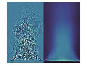
From a modelling perspective, flow visualisation (figure 1) indicates that the turbulent flow above the plate consists of three distinct regions, as shown schematically in figure 2: a predominantly horizontal region of inward flow from the edges towards the plate centre, which we refer to as a horizontal plume, labelled A; a central transitional region where these plumes merge, labelled B, and within which the flow is turned vertically; and a plume-like region of predominantly vertical flow, labelled C, formed as buoyant fluid rises from region B.
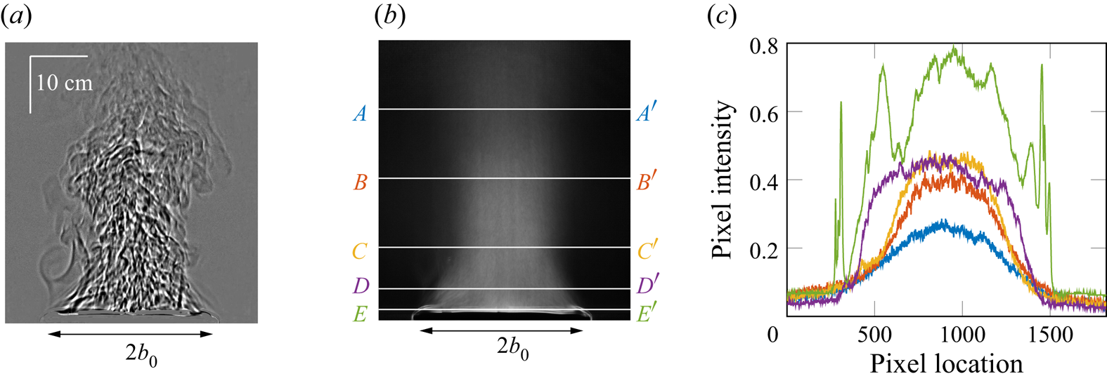
Figure 1. Shadowgraph images of the turbulent airflow above a rectangular heated plate of aspect ratio 6.6 at  $Ra \approx 3 \times 10^{10}$: (a) instantaneous and (b) time averaged. (c) Intensity profiles on $AA'$ (blue), $BB'$ (red), $CC'$ (yellow), $DD'$ (purple) and $EE'$ (green).
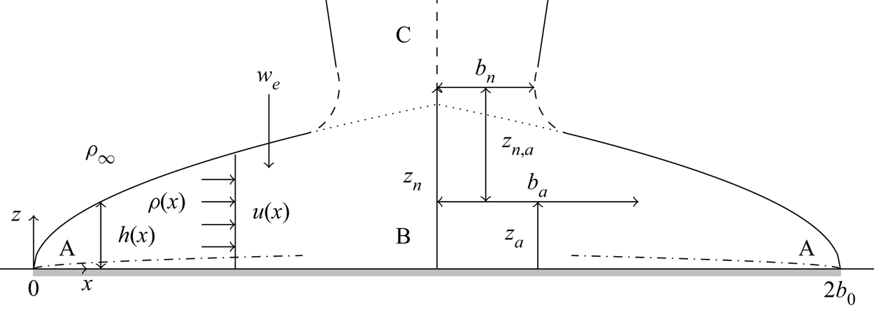
Figure 2. Representation of the mean flow above a plate on  ${z=0}$ emitting a uniform heat flux $q$ (Wm $^{-2}$) over $x \in [0, 2b_0]$ and $y\in [-\infty,\infty ]$ into an environment of density $\rho _\infty$. Here A denotes a horizontal plume with velocity $u$, height $h$ and density $\rho$; B denotes the transitional region in which the horizontal plumes converge to form a vertical plume, labelled C. The height and half-width of the plume neck ( $z_n$ and $b_n$) and apparent source ( $z_a$ and $b_a$) are indicated. Dot-dash lines (– ${\cdot }$ – ${\cdot }$) indicate slender boundary layers.
The nature of the horizontal plume A is determined by the Prandtl  $Pr$ and Rayleigh ${Ra= g\beta q (2b_0)^4/\mathcal {K}\nu \kappa }$ numbers (Fan et al. Reference Fan, Zhao, Torres, Xu, Lei, Li and Carmeliet2021), where $g$ is the gravitational acceleration and $\beta, \nu, \kappa$ and $\mathcal {K}$ are, respectively, the coefficient of thermal expansion, the kinematic viscosity, thermal diffusivity and thermal conductivity of the fluid. Our focus is primarily on thermal plumes in air, for which $Pr \approx 1$. The horizontal plume is observed to be laminar for $Ra\leq O(10^3)$ (Fan et al. Reference Fan, Zhao, Torres, Xu, Lei, Li and Carmeliet2021) and the bulk of the existing work has focused on this case, using boundary layer theory to estimate the heat transfer from the plate (Stewartson Reference Stewartson1958; Gill, Zeh & del Casal Reference Gill, Zeh and del Casal1965; Rotem & Claassen Reference Rotem and Claassen1969; Pera & Gebhart Reference Pera and Gebhart1973a; Ackroyd & Lighthill Reference Ackroyd and Lighthill1976; Kozanoglu & Lopez Reference Kozanoglu and Lopez2007; Jiang, Nie & Xu Reference Jiang, Nie and Xu2019b). Kitamura et al. (Reference Kitamura, Mitsuishi, Suzuki and Kimura2015) found the critical value of $Ra_{crit}=5\times 10^5$ for the transition to turbulence for a plate of aspect ratio $L/b_0=6$. In our experiments (§ 4), $L/b_0=6.6, Ra=O(10^{10})$ and we observed the flow to be turbulent.
By contrast, theoretical models based on classic plume theory have been developed for vertical, turbulent plumes C above high-aspect-ratio rectangular area sources with non-zero specific source momentum flux ( $M_0 \neq 0$), and plume behaviour classified (van den Bremer & Hunt Reference van den Bremer and Hunt2014) in terms of the source Richardson number
 \begin{equation} \varGamma_0 = \mathcal{C}\frac{B_0 Q_0^3}{M_0^3}. \end{equation}
In (1.1),  $B_0$ and $Q_0$ are the physical fluxes per unit length ( $y$ direction, figure 2) of buoyancy and volume, respectively, at the physical source, and $\mathcal {C}$ is a constant. The significance of $M_0 \neq 0$ is that the source supplies fluid, whereas for the heated plate, $M_0 \equiv 0$. van den Bremer & Hunt (Reference van den Bremer and Hunt2014) consider top-hat profiles for the cross-stream variation of buoyancy and velocity, defining $\mathcal {C}=(2\alpha _h)^{-1}$, where $\alpha _h$ is the horizontal entrainment coefficient for a well-established, i.e. pure, vertical planar plume. ‘Lazy’ or buoyancy-dominated releases, for which a heated plate represents the limiting case given $M_0 \equiv 0$, correspond to $\varGamma _0 > 1$. The virtual origin of a plume is the location $z=z_{avs}$ of a line source of buoyancy flux only that gives rise to the same asymptotic behaviour as above the physical source at $z=0$. For a plume that is lazy at source, it is readily shown (van den Bremer & Hunt Reference van den Bremer and Hunt2014) that the virtual origin is at
 \begin{equation} \frac{z_{avs}}{b_0}=
\frac{\mathcal{F}(\varGamma_0)-3}{3 \alpha_h
\varGamma_0^{1/3}} \quad \mbox{where}\ \mathcal{F}(\varGamma_0)=\sum_{j=1}^{j=\infty}
\left(\left(\prod_{i=1}^{i=j}(i-2/3)\right)
\frac{\left(\dfrac{\varGamma_0-1}{\varGamma_0}\right)^{j}}{(\,j-1/3)j!}\right),
\end{equation}
\begin{equation} \frac{z_{avs}}{b_0}=
\frac{\mathcal{F}(\varGamma_0)-3}{3 \alpha_h
\varGamma_0^{1/3}} \quad \mbox{where}\ \mathcal{F}(\varGamma_0)=\sum_{j=1}^{j=\infty}
\left(\left(\prod_{i=1}^{i=j}(i-2/3)\right)
\frac{\left(\dfrac{\varGamma_0-1}{\varGamma_0}\right)^{j}}{(\,j-1/3)j!}\right),
\end{equation}
and for  $\varGamma _0 > 2$, the plume contracts to a minimum half-width $b_n$, or neck, where locally $\varGamma =\varGamma _n=2$, at a height $z_n$ where
 \begin{align} \frac{b_n}{b_0}=\left(\frac{\varGamma_n}{\varGamma_0}\right)^{2/3} \left(\frac{\varGamma_0-1}{\varGamma_n-1}\right)^{1/3} \quad \mbox{and} \quad \frac{z_{n}}{b_0}= \frac{(\varGamma_0-1)^{1/3}}{3 \alpha_h \varGamma_0^{2/3}}\int^{\varGamma_0}_2 \frac{\mathrm{d}Y}{Y^{1/3}(Y-1)^{4/3}}. \end{align}
Solutions (1.2) and (1.3) are based on the assumption of an invariant entrainment coefficient. Modelling the flow above a heated plate using plume theory is problematic given  ${M_0\equiv 0}$ and, thus, $\varGamma _0$ is undefined. Alternatively, if one considers the limit ${M_0\to 0}, {\varGamma _0\to \infty }$ and the plume is predicted to contract to a width of zero (1.3a) and ${z_n/b_0\to 0}$ (1.3b), i.e. the neck is coincident with the physical source. Moreover, from (1.2), ${z_{avs}/b_0\to 0}$, which suggests that the physical plume can be represented as that from the virtual line source $(B_0>0,Q_0=M_0=0)$ at the same elevation as the physical source. This contradictory prediction is clearly non-physical. Evidently, existing plume models (Kaye Reference Kaye2008; Woods Reference Woods2010; Hunt & van den Bremer Reference Hunt and van den Bremer2011) cannot accurately capture the bulk features of the time-averaged turbulent flow above a heated plate and an improved description of the near-plate plume flow is required, providing motivation for the current study.
Only in the past twenty five years has information on the large-scale turbulent motion above a heated plate at high  $Ra$ been reported. Kitamura, Chen & Kimura (Reference Kitamura, Chen and Kimura2001) focused on laminar-turbulent transition, with flow visualisation revealing a near-plate horizontal convergent flow that turns to become vertical. Tsitsopoulos (Reference Tsitsopoulos2013) considered theoretically the axisymmetric flow above a heated disc, however, this model became intractable due to mathematical difficulties attributed to the geometry. We initially adopt his approach to model the flow above a rectangular plate (§ 2). Notably, the recent review of Fan et al. (Reference Fan, Zhao, Torres, Xu, Lei, Li and Carmeliet2021) cites no examples of previous theoretical studies on the turbulent case.
Our approach is as follows. In § 2 we develop the first theoretical description of the attached horizontal plumes and successfully avoid the aforementioned contradiction(s). We model the horizontal plume growing from one edge of the plate in isolation, assuming the mean flow is two dimensional, and solve analytically the resulting conservation equations. By assuming that the vertically rising plume-like flow is supplied at its apparent source by a horizontal plume growing from each edge of the heated surface, in § 3 we characterise theoretically the apparent source. With these predictions, we use the theory for planar plumes of van den Bremer & Hunt (Reference van den Bremer and Hunt2014) to predict the neck height above the heated plate. In § 4 we detail shadowgraph experiments and temperature measurements that are compared with the theory of §§ 2 and 3, confirming that our model captures the observed flow well and that the plume from a heated plate may now be described by applying classic plume theory from the apparent source we identify.
2. Governing equations for the horizontal plume
Consider the horizontal plume on a heated plate of width  $2b_0$ that extends infinitely in the spanwise direction ( $y$ axis into the page, figure 2). A steady uniform heat flux $q > 0$ (Wm $^{-2}$) is supplied on $z=0$ for $0\leq x\leq 2b_0$, and $q=0$ on $z=0$ for $x<0$ and $x>2b_0$. These unheated regions are assumed to be perfectly insulated from the heated region and remain isothermal with temperature identical to the surrounding ambient. The environment for $z>0$ is unbounded, of uniform density $\rho _\infty$ and is treated as an ideal gas. The heat flux is equivalent to a uniform buoyancy flux of $F=(g/\rho _\infty T_\infty c_p)q$ per unit area, where $c_p$ denotes the specific heat capacity. The convective flow so driven is treated as incompressible, fully turbulent and independent of the Reynolds number, so the effects of molecular diffusion and viscosity are neglected. While we acknowledge that the effects of viscosity play a key role in the development of slender boundary layers within the near-plate region of A, we neglect altogether the presence of boundary layers and any associated loss of momentum in the horizontal plume due to contact with the plate; our solutions therefore do not satisfy the no-slip condition and velocities may be interpreted as those outside the boundary layer. Whilst a simplifying assumption, the results of Rotem & Claassen (Reference Rotem and Claassen1969) and Pera & Gebhart (Reference Pera and Gebhart1973b) would appear to aid us in justifying such an approach. Indeed, they found that the boundary layer growing from the plate edge separated when the local Grashof number $Gr_x=g\beta x^3{\rm \Delta} T/\nu ^2\approx 100$, where ${\rm \Delta} T$ is the temperature difference between the plate surface and the ambient. For the experimental conditions we consider, separation is therefore expected at $x\approx 5$ mm, i.e. after only ${\sim }3\,\%$ of the plate half-width of $b_0 \sim 152$ mm, meaning that the majority of the flow we are modelling is not expected to be a classic boundary layer flow but a convective turbulent flow. Accordingly, given a primary aim is to establish how bulk entrainment and plume merger (§ 3) ultimately control the ‘apparent source’ conditions for C, we make the simplifying assumption that the cross-stream profiles of both mean horizontal velocity $u(x)$ and density $\rho (x)$ are uniform.
The mean quantities considered are those averaged in time and spatially in  $y$. The interface at $z=h(x)$ is gravitationally unstable and subject to shear. The resulting Rayleigh–Taylor instabilities and turbulent engulfment give rise to mixing at this interface, causing a net downward transport of fluid, with velocity $w_e$ and density $\rho _\infty$, into the plume (region A, figure 2). The mean height of the plume $h(x)$ thereby increases in the $x$ direction. Adapting the entrainment assumption, cf. Taylor (Reference Taylor1945) for vertical plumes, the entrainment velocity $w_e$ is proportional to a local characteristic velocity in the plume, i.e. $w_e=-\alpha _v u$, where $\alpha _v>0$ is the vertical entrainment coefficient. As confirmed in § 4.1.4, it is to be expected that $\alpha _v > \alpha _h$ due to both the gravitational and shear instabilities at the horizontal plume perimeter, compared with just the shear instability at the vertical plume boundary. Under these assumptions, approximating the fluid as a Boussinesq, ideal gas it is readily shown (Appendix A) that statements of conservation of mass, specific momentum and energy reduce to
 \begin{equation} \frac{\mathrm{d}Q}{\mathrm{d} x} = \alpha_v \frac{M}{Q}, \quad \frac{\mathrm{d}M}{\mathrm{d} x} = \frac{1}{2}\frac{\mathrm{d}}{\mathrm{d} x} \left(\frac{BQ^3}{M^2}\right) \quad \mbox{and} \quad \frac{\mathrm{d}B}{\mathrm{d} x} = F, \end{equation}
respectively, where  $Q=uh, M=u^2h, B=g'uh$ and the reduced gravity $g'=g(\rho _\infty -\rho )/ \rho _\infty$. The boundary conditions are $Q=M=B=0$ at $x=0$. The equations for volume flux $Q$ and buoyancy flux $B$, (2.1a) and (2.1c), are identical to those for a vertical wall plume (Cooper & Hunt Reference Cooper and Hunt2010). The difference in the momentum flux equation (2.1b) is due to the fact that the increase in specific momentum flux $M$ in the horizontal plume is driven by a horizontal pressure gradient, whereas in a wall plume it is driven by buoyancy. While there is no naturally arising characteristic length scale for the horizontal plume flow above a semi-infinite plate, we have elected below to non-dimensionalise using the physical plate half-width, $b_0$, given our ultimate goal concerns the plume above a plate of finite width. With lengths scaled on $b_0$, indicated with hatted variables, we introduce the dimensionless fluxes $\hat {Q}, \hat {M}$ and $\hat {B}$ via
 \begin{equation} \hat{Q} = \frac{Q}{\alpha_v b_0 U}, \quad \hat{M} = \frac{M}{\alpha_v b_0 U^2}, \quad \hat{B} = \frac{B}{b_0 F}, \end{equation}
where  $U$ is a horizontal velocity scale. Accordingly, (2.1) and the boundary conditions reduce to
 \begin{equation} \frac{\mathrm{d}\hat{Q}}{\mathrm{d}\hat{x}} = \frac{\hat{M}}{\hat{Q}}, \quad \frac{\mathrm{d}\hat{M}}{\mathrm{d}\hat{x}} = \frac{b_0 F}{2U^3}\frac{\mathrm{d}}{\mathrm{d}\hat{x}} \left(\frac{\hat{B}\hat{Q}^3}{\hat{M}^2}\right), \quad \frac{\mathrm{d}\hat{B}}{\mathrm{d}\hat{x}} = 1, \end{equation}
and  $\hat {Q}=\hat {M}=\hat {B}=0$ on $\hat {x}=0$. Defining $U$ as the velocity at the centre of the plate, i.e. $U=(b_0F/2)^{1/3}$ as confirmed in (2.6), the governing equations are rendered independent of the source conditions. Equations (2.3b) and (2.3c) may be integrated directly, thence
 \begin{equation} \frac{\mathrm{d}\hat{Q}}{\mathrm{d}\hat{x}}=\frac{\hat{M}}{\hat{Q}}, \quad \frac{\hat{B}\hat{Q}^3}{\hat{M}^3} = 1 \quad \mbox{and} \quad \hat{B} = \hat{x}. \end{equation}
That the ratio of fluxes  $\hat {B}\hat {Q}^3/\hat {M}^3$, a Richardson number for the horizontal plume, is invariant enables comparisons to be drawn with the analogous dynamical invariance in the far field of a vertical plume. Moreover, (2.4c) indicates, as expected for a uniformly distributed buoyancy input, that the buoyancy flux increases linearly with $\hat {x}$. Solving (2.4) we obtain
 \begin{equation} \hat{Q} =
\tfrac{3}{4}\hat{x}^{4/3}, \quad \hat{M} =
\tfrac{3}{4}\hat{x}^{5/3} \quad \mathrm{and} \quad \hat{B} =
\hat{x},
\end{equation}
\begin{equation} \hat{Q} =
\tfrac{3}{4}\hat{x}^{4/3}, \quad \hat{M} =
\tfrac{3}{4}\hat{x}^{5/3} \quad \mathrm{and} \quad \hat{B} =
\hat{x},
\end{equation}
or, in terms of the height, velocity and reduced gravity of the horizontal plume
 \begin{equation} h = \frac{3}{4}\alpha_v x, \quad u = U\left(\frac{x}{b_0}\right)^{1/3} \quad \mathrm{and} \quad g'=\frac{4}{3\alpha_v} \left(\frac{2F^2}{x}\right)^{1/3}. \end{equation}
That  $u(x=b_0)=U$ confirms $U=(b_0F/2)^{1/3}$ as a natural choice for the velocity scale. The linear dependence of plume height (2.6a) and the singular behaviour $g'\to \infty$ as $x\to 0^+$ (2.6c) are assessed in § 4.
3. Source conditions for the vertical plume
The Richardson number  $\varGamma _a$, cf. (1.1), that characterises the ‘apparent’ source governs the classification and, thereby, behaviour of the vertical plume C. The vertical fluxes of volume, specific momentum and buoyancy at the apparent source are taken to be ${(Q_a,M_a,B_a)}={(2Q_c,2\lambda M_c,2B_c)}$, where the fluxes in the horizontal plumes (2.5) are evaluated on the centreline, viz.
 \begin{equation} Q_c=\tfrac{3}{4}\alpha_v
b_0 U, \quad M_c=\tfrac{3}{4}\alpha_v b_0 U^2, \quad B_c=b_0
F.
\end{equation}
\begin{equation} Q_c=\tfrac{3}{4}\alpha_v
b_0 U, \quad M_c=\tfrac{3}{4}\alpha_v b_0 U^2, \quad B_c=b_0
F.
\end{equation}
In other words, the combined volume fluxes of the horizontal plumes at the centre of the plate form the apparent source volume flux and we have assumed that the vertical momentum flux at the apparent source should scale so as to be proportional to the magnitude of the horizontal momentum (evaluated on the centreline), an assumption routinely applied to plume-boundary impingements (Jiang et al. Reference Jiang, Creyssels, Hunt and Salizzoni2019a).
Without further scaling, these fluxes lead to an invariant Richardson number of  $B_aQ_a^3/M_a^3 = 4/\lambda ^3$. Given our goal is to apply the results of plume theory from this apparent source, we rescale so as to be consistent with that required for a pure plume to have a Richardson number of unity. Accordingly, with reference to (1.1) with $\mathcal {C}=(2\alpha _h)^{-1}$,
 \begin{equation} \varGamma_a = \frac{B_a Q_a^3}{2\alpha_h M_a^3} = \frac{b_0F}{\alpha_h\lambda^3U^3} = \frac{2}{\alpha_h\lambda^3}. \end{equation}
 Given measurements indicate that  $\alpha _v\approx 1.2$ (§ 4.1.4), from (2.6), $h\approx b_0$ at $x=b_0$ and, thus, it is not reasonable to treat the heated plate as a $\varGamma _0=2/\alpha _h\lambda ^3$ source at $z=0$ using plume theory; indeed, our observations (§ 4) show that the neck is higher and narrower than that predicted based on such a treatment. Thus, we proceed by predicting the apparent source height, $z_a$, half-width, $b_a$ (figure 2), and its virtual origin location, $z_{avs,a}$, that would match the observed $b_n$ and $z_n$. To do this, we relate $z_a, b_a$ and $z_{avs,a}$ to the quantities we can directly measure, $b_n$ and $z_n$, and infer $z_{avs}$ (§ 4) using the relationship derived below.
On dimensional grounds, we define, for the constants  $\{k,m,p\}>0$,
 \begin{equation} \hat{b}_n=k, \quad \hat{z}_n=m \quad \mbox{and} \quad \hat{z}_{avs}={-}p. \end{equation}
Given  $\varGamma _n=2$, the ratio of the neck and apparent source half-widths is, from (1.3),
 \begin{equation} \frac{b_n}{b_a}=\left(\frac{\varGamma_n}{\varGamma_a} \right)^{2/3}\left(\frac{\varGamma_a-1}{\varGamma_n-1}\right)^{1/3} \implies \hat{b}_a = k(\alpha_h\lambda^3(2 - \alpha_h\lambda^3))^{{-}1/3}. \end{equation}
The location of the apparent source  $\hat {z}_a$ is given by the distance between the actual and apparent neck heights, i.e. $\hat {z}_a=\hat {z}_n-\hat {z}_{n,a}$ (figure 2), hence,
 \begin{equation} \hat{z}_a=m-kI \quad \mbox{where} \ I = \frac{1}{2^{2/3}3\alpha_h} \int_2^{2/(\alpha_h\lambda^3)} \frac{{\rm d}Y}{Y^{1/3}(Y-1)^{4/3}}, \end{equation}
cf. (1.3). If the plume from the apparent source is an accurate model for the far-field data, the experimentally observed virtual origin, measured by linearly tracing the far-field plume perimeter back to a line of intersection, and the theoretical apparent virtual origin will be coincident. In other words, if the model is accurate, the far-field perimeter of the plume above the heated plate, and that of a theoretical plume issuing from the apparent source will be the same. The measured virtual origin is determined relative to the physical source (i.e. the physical plate), while the apparent virtual origin is located relative to the apparent source. The virtual origin for the plume from the apparent source,  $\hat {z}_{avs,a}$, relative to the apparent source is therefore given by the distance between the virtual origin location relative to the plate and the apparent source location, i.e. $\hat {z}_{avs,a}=\hat {z}_{avs}-\hat {z}_a$. Equating this expression with (1.2) and using (3.5) gives
 \begin{equation} \hat{z}_{avs,a} = kI-p-m={-}\frac{k}{3}\frac{3-\mathcal{F} (\varGamma_a)}{[\alpha_h^4\varGamma_a(2-\alpha_h)]^{1/3}}. \end{equation}
While  $\varGamma _a$ has been established above, $b_a$ and $z_a$ must be inferred from experimental measurements of the neck width, neck height and asymptotic virtual origin location, parameterised by $k, m$ and $p$, respectively. Thus, in what follows we report on measurements of $k$ and $m$, and predict the value of $p$. This choice was made as $p$ would need to be established from the far-field gradient of the width. In contrast, $k$ and $m$ can be established solely from measurements made nearer to the source – this near-field measurement approach offers significant advantages for the study of convection above large-aspect-ratio plates given the true far field is often not accessible to measurement.
Throughout this section the constant of proportionality,  $\lambda$, was retained in the analysis, however, we set $\lambda = 1$ in § 4. Here $\lambda = 1$ corresponds to the least lazy apparent source. However, it transpires that the question of identifying the most appropriate value for $\lambda$ is not problematic as knowledge of the neck location and width (empirically observed constants in the model we develop) determines the plume perimeter below that height. For $0 < \lambda < 1$, the apparent source is increasingly lazy, wider and further below the neck (closer to the plate) and, as such, the predicted plume perimeter is extended nearer to the plate, but forms a smooth continuation of the predicted plume perimeter for $\lambda = 1$.
4. Experimental investigation
The heat source was a rectangular brass plate ( $L=1000\pm 1$ mm, $2b_0=305\pm 1$ mm, thickness $6\pm 0.1$ mm) mounted directly atop four electrically heated discs (diameter $\phi =154$ mm, maximum heat output 1 kW) aligned along the plate centreline with centres at 232 mm spacing. Shadowgraph experiments were conducted in air for ${2.6 \times 10^{10}< Ra <8.0 \times 10^{10}}$, a range achieved by varying the plate temperature. Temperature profile measurements were made for $Ra \approx 4 \times 10^{10}$. The plumes were interrogated by means of flow visualisation for $\hat {z}\lesssim 3$ (§ 4.0.1) and direct temperature measurements for ${\hat {z}\lesssim 4}$ (§ 4.0.2). Yokoi (Reference Yokoi1960) established that the plume from a slender rectangular source departs from the two-dimensional scaling ( $g'\sim z^{-1}$) toward the axisymmetric scaling ( $g'\sim z^{-5/3}$) at elevations of ${z/L = 6-7}$; given $\hat {z}=4$ corresponds to $z/L \approx 0.6$, our measurements are firmly within the region in which two-dimensional flow is to be expected. The plate temperature was measured using type-K thermocouples (Omega Engineering (OE), $\phi =$0.025 mm, response time $t_r=0.15$ s), surface mounted at $(x,y)=(40,30)$, (40,270), (153,150) and (153,390) mm ( $\pm 1$ mm). Across all experiments, the time-averaged ensemble mean surface temperature spanned ${\langle {T}_p\rangle =69.2\unicode{x2013}125.2^\circ {\rm C}} (\pm 0.1^\circ {\rm C})$ and the instantaneous room temperature $T_\infty =23.4\unicode{x2013}25.1^\circ {\rm C} (\pm 0.1^\circ {\rm C})$; the $\pm$ range given for $\langle T_p \rangle$ and $T_\infty$ was dictated by the precision of the instrument. The variation of temperature recorded across the plate is given in table 1, Appendix B. Accordingly, we take the properties of air at ${T_\infty = 297}$ K and standard atmospheric pressure (1.01325 bar) (Cimbala & Çengel Reference Cimbala and Çengel2008). Finally, we note that van den Bremer & Hunt (Reference van den Bremer and Hunt2014) identify the non-dimensional vertical length over which non-Boussinesq effects are important scales as $\mathcal {L}_{NB-B} \sim (4F^2/(b_0g^3\alpha _h^2))^{1/3}$. Whilst expressed as a length scale, $\mathcal {L}_{NB-B}$ incorporates effects of both the size and strength of the buoyancy source. For a typical shadowgraph experiment, $\mathcal {L}_{NB-B} \approx 0.1$ (taking $g=9.81$ ms $^{-2}$); given this length scale is measured from the virtual origin at $\hat {z}_{avs}\approx -1$ (see § 4.1.3), the vertical plume is expected to be Boussinesq at all heights.
4.0.1 Shadowgraph
The flow was visualised using direct shadowgraphy in diverging light (Settles Reference Settles2001). Light rays passing through each  $x\unicode{x2013}z$ plane are continuously deflected due to the inhomogeneous density field. Each shadowgraph image therefore captures the superposition of the deflections over all $x\unicode{x2013}z$ planes between light source and camera, and thereby provides a spanwise integrated view of the flow. Images were recorded at 12.5 frames per second using a JAI SP-5M CCD camera and Kowa 16 mm lens. Instantaneous images so obtained, figure 1(a), show turbulent motion above the plate, an increase in the depth $h$ of the horizontal plume with $x$ and the contraction in the vertical flow to a neck.
A characteristic time scale for the horizontal plume is
 \begin{equation} \tau = \frac{b_0}{U} = \left(\frac{2b_0^2c_pT_\infty\rho_\infty}{qg}\right)^{1/3} \approx 1 \mbox{s}. \end{equation}
Each experiment was recorded for a period of  $90\ {\rm s} \gg \tau$, and the corresponding 1125 instantaneous images combined to produce a single time-and-space averaged image, cf. figure 1(b). For $\hat {z} \gtrsim 0.2$, the intensity distribution is near Gaussian for each row of the resulting image (the coefficient of determination ${R^2=\{0.985, 0.985, 0.976, 0.937\}}$ for profiles $AA'$ to $DD'$, respectively) and, hence, the plume perimeter was defined as the locations $x=b_{lhs}$ and $x=b_{rhs}$, at which the intensity had fallen to $1/\sqrt {e}$ of the row maximum, where $\ln (e)=1$. Accordingly, the normalised plume half-width was defined as $\hat {b} = (b_{rhs} - b_{lhs})/2b_0$.
4.0.2 Temperature measurements
Cross-stream profiles of time-averaged temperature  $\bar {T}(x,z)$ at $y=L/2$ were obtained by horizontally traversing a type-K thermocouple (OE, $\phi =0.25$ mm, ${t_r< 1}$ s) from ${x = \{-60, 370\}}$ mm in $10$ mm increments at elevations of ${z = \{0, 5 ,10\}}$ mm, and from $z = \{20, 290\}$ mm in $10$ mm increments. Temperatures at each location were sampled by the datalogger every second for ${\sim }60\tau$, from which $\bar {T}$ was calculated. Consistent with shadowgraph experiments, the plume perimeter was defined as the $x$ locations at which $\bar {T}=\bar {T}_m/\sqrt {e},$ where $\bar {T}_m$ denotes the maximum time-averaged temperature at that elevation.
4.1 Results
4.1.1 Width measurements
Figure 3(a) plots profiles of the normalised half-width inferred from 21 shadowgraph experiments with different  $\bar {T}_p$, and their ensemble median. The plate temperature for each of the shadowgraph experiments is detailed in Appendix B. Half-widths obtained from the temperature traverses are overlaid as crosses. While values differ, both approaches capture the same general trends; the morphology of the high- $Ra$ plume is invariant and is characterised by a far-field linearly expanding region (§ 4.1.2), a height at which the plume is narrowest (§ 4.1.3) and a near-field linearly contracting region (§ 4.1.4).
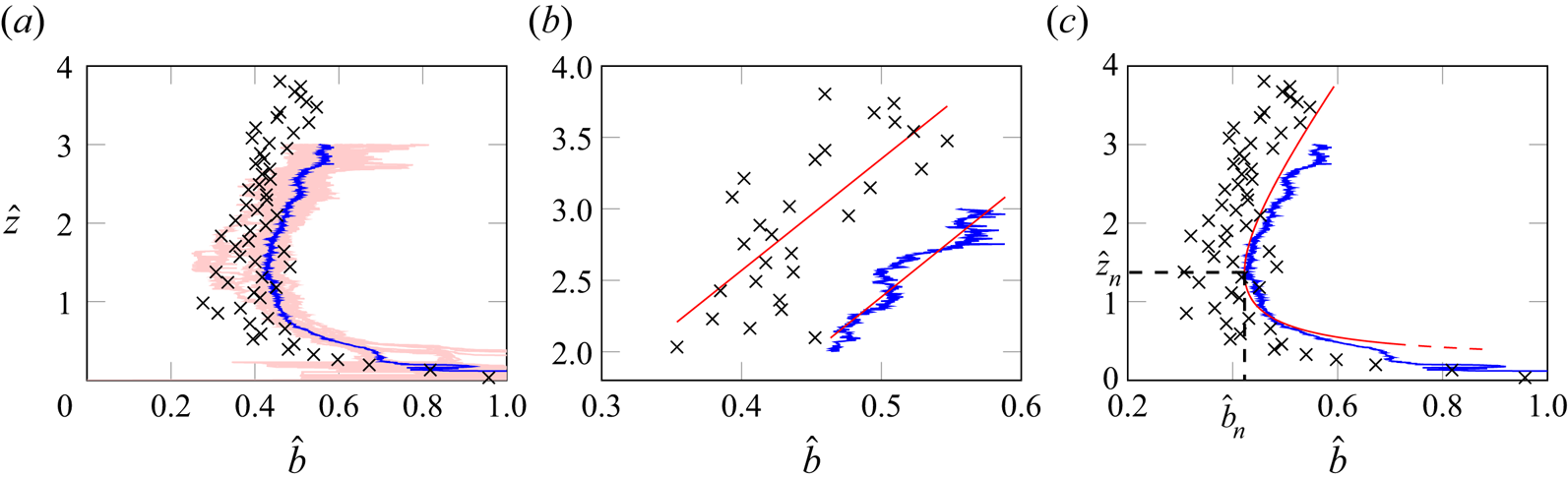
Figure 3. (a) Normalised half-width from: (—–, light red) 21 shadowgraph experiments; (—–, blue) the ensemble median (from which  $\hat {z}_n =1.37, \hat {b}_n = 0.423$, as marked on (c)); ( $\times$, black) temperature data. (b) Linear best fits to data in (a) for $\hat {z}>2$; gradients are 7.82 (temperature) and 7.89 (shadowgraph), with correlation coefficients 0.720 and 0.945, respectively. (c) Prediction of our model for an impingement region of: (—–, red) zero width; (- - - -, red) finite width with an aspect ratio of 2. The shadowgraph measurements were recorded for $2.6 \times 10^{10}< Ra <8.0 \times 10^{10}$ and the temperature traverses for $Ra \approx 4 \times 10^{10}.$
The shadowgraph data are noisy immediately above the plate (figure 3(a) for  $\hat {z} \lesssim 0.35$) and this is evident in the ensemble average. The cause is twofold: firstly, as the shadowgraphy was in diverging light, the magnification of the flow above the plate edge nearest the light source is $15\,\%$ greater than that above the farthest edge (as estimated from Settles (Reference Settles2001) given the light source and plate centreline were 911 and 196 cm from the visualisation screen, respectively) and this creates some uncertainty as to the plate location in an image; secondly, the intensity profiles here are not Gaussian, cf. profile $EE'$ in figure 1(b,c), and, as such, the thresholding of the intensity breaks down.
Figures 4(a) and 4(b) plot the dimensionless neck width and neck height, respectively, against non-dimensional plate temperature,  $\theta _p=(\langle T_p \rangle - T_\infty )/T_\infty$. It is clear that both $\hat {b}_n$ and $\hat {z}_n$ are approximately constant over the range of $\theta _p$ measured. For each shadowgraph experiment, $\hat {b}_n$ was taken as the smallest value of $\hat {b}$, and $\hat {z}_n$ as the height at which this minimum occurred. The greater spread observed in the neck height measurements, compared with the neck width measurements, is expected; near the neck $\mathrm {d}\hat {b}/\mathrm {d}\hat {z} \to 0$, so measurements of neck width are relatively robust to errors in the shadowgraph, whereas the neck height measurements are more sensitive (there is a large range of values of $\hat {z}$ with $\hat {b} \approx \hat {b}_n$). Transition to turbulence in the horizontal plume could provide an explanation for the increased spread in the measurements for $\theta _p \lesssim 2.3$.
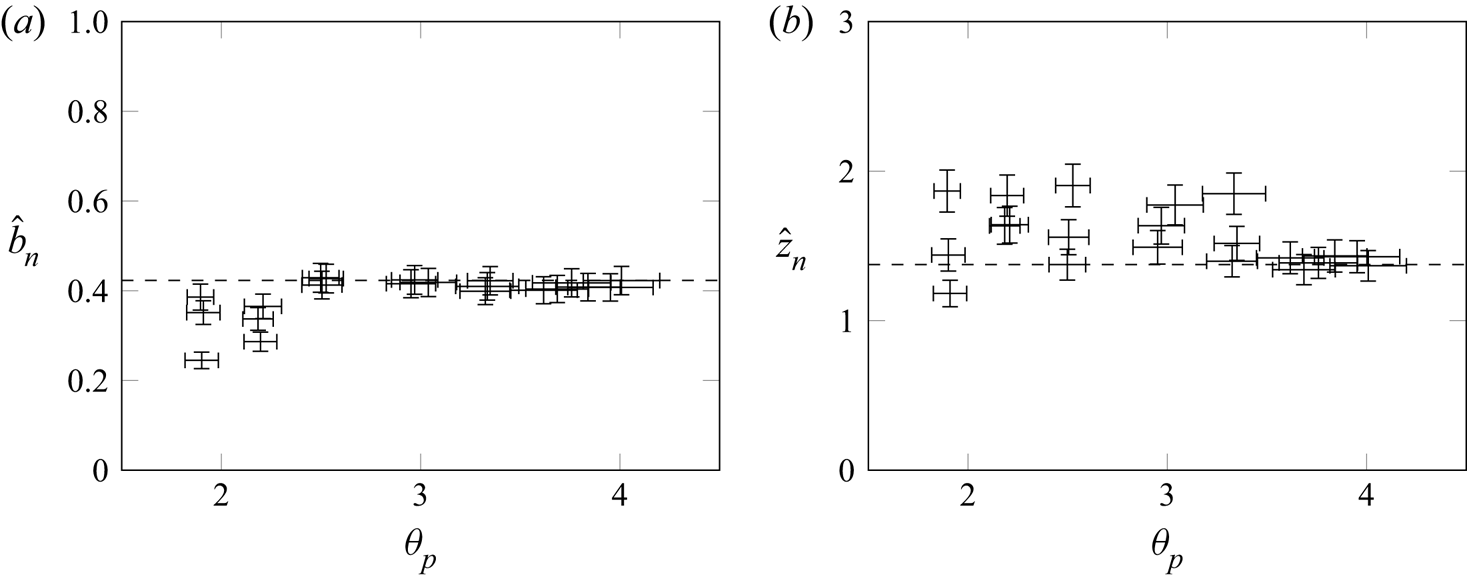
Figure 4. (a) Normalised neck width versus plate temperature; - - - - neck width  ${\hat {b}_n = 0.423}$ corresponding to the ensemble-averaged shadowgraph data. (b) Normalised neck height versus plate temperature; - - - - neck height ${\hat {z}_n = 1.37}$ corresponding to the ensemble-averaged shadowgraph data. Horizontal error bars show the standard error of the mean ( $\sigma /\sqrt {N}$), where $\sigma$ is the standard deviation and $N$ the number of observations. Vertical error bars reflect the 15 % difference in magnification along the plate.
4.1.2 Far-field region
Irrespective of the actual, or apparent, source Richardson number,  ${\varGamma \to 1}$ as ${\hat {z} \to \infty }$ (van den Bremer & Hunt Reference van den Bremer and Hunt2014), a dynamically invariant region where the entrainment coefficient $\alpha _h$ can be inferred from the constant growth rate of the vertical plume. While the Richardson & Hunt (Reference Richardson and Hunt2022) assessment of the literature on line plumes and their own independent measurements based on the plume-induced flow show $\alpha _h\approx 0.11$, for completeness we estimate $\alpha _h$ from our own measurements. Figure 3(b) plots the half-width data and linear best fits for ${\hat {z} > 2}$. Given the cross-stream profiles are approximately Gaussian (see profiles $AA'$– $DD'$, figure 1), ${\alpha _h = (\sqrt {\pi }/2)\mathrm {d}\hat {b}/\mathrm {d}\hat {z}}$ (van den Bremer & Hunt Reference van den Bremer and Hunt2014) from which the respective gradients lead to ${\alpha _h \approx 0.113}$ (temperature data) and $0.112$ (shadowgraph data). That these estimates agree closely with the established value provides confidence in our data and, moreover, we may assert that the shadowgraph offers a robust approach for interrogating this source geometry.
Substituting  $\alpha _h = 0.11$ into (3.2) and (3.6) gives
 \begin{equation} \varGamma_a=18.2, \quad I=2.16 \quad \mbox{and} \quad p + m = 6.51k, \end{equation}
to three significant figures.
4.1.3 Apparent source
Substituting our empirical measurements  $k=0.423$ and $m=1.37$, figure 3(c), into (3.4) and (3.5), the half-width and location of the apparent source are, respectively,
 \begin{equation} \hat{b}_a = 0.423\times1.69 = 0.715 \quad \mbox{and} \quad \hat{z}_a = 1.37 - (0.423\times2.16) = 0.456, \end{equation}
to three significant figures. Given  $b_0>0$ and $Q_0 \equiv 0$ the heated plate was anticipated to produce a contracting plume and, hence, it was to be expected that (i) $b_a/b_0<1$ (4.3) and (ii) $\hat {z}_a < \hat {z}_n$ given previous results show $\varGamma \approx 1$ above the neck. Additionally, compatibility with $\varGamma _a = 2/\alpha _h$ (given $\lambda =1$), as predicted by our theory, requires $p = (6.51\times 0.423) - 1.37 = 1.38$ (from (4.2c) with ${\alpha _h=0.11}$). Figure 3(c) overlays the perimeter predicted by the classic model of van den Bremer & Hunt (Reference van den Bremer and Hunt2014) for a plume emanating from our prediction of the apparent plume source ( $b_a = 0.715b_0, z_a = 0.456b_0, \varGamma _a = 18.2$) with the widths inferred from temperature measurements, and the ensemble median shadowgraph data. The data are well described by this approach, notably our predicted virtual origin location ( $-p=-1.38$) is within $12\,\%$ of the measured value – the latter given by the intercept of the trendline in figure 3(b) with the vertical axis, ${\hat {z}_{avs}=-p=-1.56}$. For $\hat {z} > \hat {z}_n, \mathrm {d}\hat {b}/\mathrm {d}\hat {z}$ increases, asymptotically approaching the far-field value. It is therefore expected that measurements at greater heights would give a smaller value for $p$. By taking the neck as the point of minimum width in the ensemble median rather than, for example, smoothing the data with a moving average, it is also expected that our value for $k=0.423$ is a lower bound. It is natural to consider whether our assuming the horizontal plumes impinge and turn at the centre of the plate, rather than in a control volume of finite width has also introduced error. The analysis considered herein can readily be extended to an impingement region of finite width; this changes the values of $b_a, z_a$ and $\varGamma _a$, but does not change the predicted plume perimeter, only extends it to lower heights, the same qualitative effect as taking a value of $\lambda$ from the range $0<\lambda <1$. The dashed red line in figure 3(c) shows this extension for an impingement region of aspect ratio 2, for which $\hat {b}_a=0.876, \hat {z}_a=0.395$ and $\varGamma _a=34.5$. Whilst there are then a multiplicity of potential apparent sources, in the interests of simplicity we advocate for use of the model (§ 3) with a zero-width impingement region, $\lambda = 1$, and apparent source
 \begin{equation} b_a = 0.72b_0, \quad z_a = 0.46b_0, \quad \varGamma_a= 18.2. \end{equation}
Despite the assumptions made, our model describes the data well, extending our predictive capability to the near field, in addition to providing ‘source’ conditions for the far field.
4.1.4 Near-source region
Figure 5(a) plots our data for the growth of the horizontal plume. Assuming symmetry about  $x=b_0$, $\hat {x} = 1 - \hat {b}$ and $\hat {h} = \hat {z}$. Both shadowgraph ( $\times$, blue) and temperature measurements ( $\times$, black) exhibit a linear evolution $\hat {h}\propto \hat {x}$, consistent with (2.6a), that extends over $0 \lesssim \hat {z} \lesssim 0.6$. The gradients of the respective trendlines (- - - -, red) are 0.960 and 0.860. For $\hat {z}=\hat {h} \lesssim 0.35$, measurements using the shadowgraph method were unreliable for the reasons outlined in § 4.1.1. Comparing ${\mathrm {d}h/\mathrm {d} x = 3\alpha _v/4}$ from (2.6a) with these gradients gives ${\alpha _v \approx 1.28}$ and ${\alpha _v \approx 1.15}$, respectively, and thereby, the average estimate
 \begin{equation} \alpha_v = 1.21. \end{equation}
Thus, near-source entrainment exceeds the far-field entrainment ( $\alpha _h \approx 0.11$) by an order of magnitude. That $\alpha _v > \alpha _h$ is consistent with previous evidence of enhanced entrainment in the near-source region of lazy plumes (Kaye & Hunt Reference Kaye and Hunt2009; Marjanovic, Taub & Balachandar Reference Marjanovic, Taub and Balachandar2017; Ciriello & Hunt Reference Ciriello and Hunt2020).
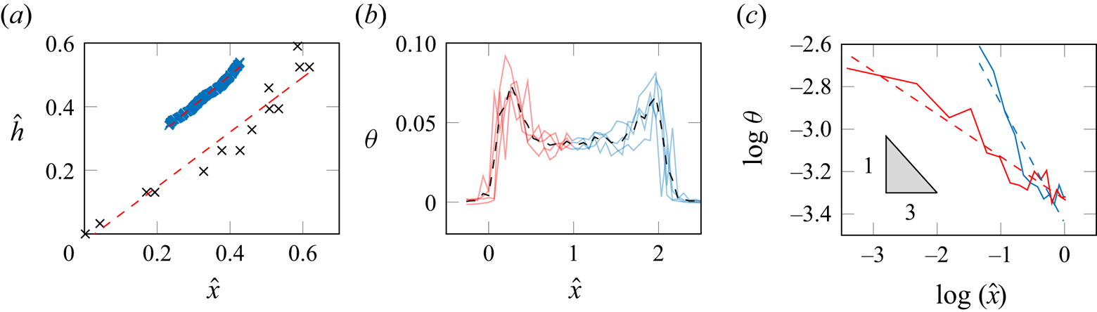
Figure 5. Horizontal plume. (a) Variation of  $\hat {h}$ with $\hat {x}$ obtained from the ensemble-averaged shadowgraph data ( $\times$, blue) and temperature measurements for $Ra \approx 4 \times 10^{10}$ ( $\times$, blue), with linear best fits to the data (- - - -, red). Profiles of $\theta$ at $\hat {z} = 0.033$ on (b) linear and (c) logarithmic axes. In (c) the solid lines show the average temperature profile between the peaks, and the dashed lines show a linear best fit.
Treating air as an ideal gas at room temperature ( $T_\infty =297$ K), $\theta =(\bar {T}-T_\infty )/T_\infty =0.023\,\hat {x}^{-1/3}$ from (2.6c); thus, $\theta \sim \hat {x}^{-1/3}$ for ${\hat {x}\in [0,1]}, \theta \sim (2-\hat {x})^{-1/3}$ for ${\hat {x}\in [1,2]}$ and behaviour is singular for $\hat {x}=\{0,2\}$. Figure 5(b) plots profiles of $\theta (\hat {x})$ recorded close to the plate and their mean. The temperatures peak close to the plate edges, giving a distinctive ‘cat-ears’ shape. Figure 5(c) replots the mean profile on $\log$- $\log$ axes; the data for $\hat {x}\in [0,1]$ has a gradient of $-0.201$ (blue) and $-0.563$ for $\hat {x}\in [1,2]$ (red). Data for $\hat {x}\in [1,2]$ has been reflected about $\hat {x}=1$ to aid comparison and as the profile is expected to be symmetric about $\hat {x}=1$. If the data are in agreement with (2.6c), a gradient of $-1/3$ is expected; our data yields an average gradient of $-0.382$. Evidently viscous effects become important as $\hat {x} \rightarrow 0^+$ and $2^-$, preventing the singular behaviour predicted.
In summary, the behaviour observed supports the predictions.
5. Conclusions
Our dual theoretical and laboratory investigation concerned the region of quasi-steady miscible Boussinesq flow in the near field above a high-aspect-ratio rectangular heated plate in quiescent surroundings. Having zero momentum flux at source, the heated plate represents the limiting case of an infinitely lazy plume source that, prior to this study, was not amenable to solution based on the application of classic plume theory.
Guided by flow visualisation in air, our thesis was (i) that the merger of two convergent horizontal flows that propagate along the plate controls the (apparent) source conditions for the classic two-dimensional plume above, and (ii) by determining these conditions plume theory may be successfully applied to capture the bulk convective flow above a heated plate. Our analytical solutions demonstrate that the two horizontal plumes grow linearly, controlled by vertical entrainment, with an associated coefficient that we measure to be  $\alpha _v = 1.2$. In this region, the temperature profile takes the form of characteristic ‘cat ears’, i.e. with a temperature peaking slightly inboard of the plate edges. Based on our findings we assert that both the far-field flow and the contracting-expanding flow in the near field, above a plate of width $2b_0$, can be modelled using plume theory applied from an apparent source of width $b_a = 0.72b_0$, located at $z_a = 0.46b_0$ and with Richardson number $\varGamma _a \approx 18$. Notably, our approach accurately captures the behaviour in the neck region; this would not be possible on modelling the plate as a line source located at a virtual origin.
The significance of this advancement to the analytic theory of turbulent plumes is in opening up its extension to an entire class of sources, namely, infinitely lazy sources, and thereby in our ability to predict the bulk convective flow established above heated (or below cooled) plates, for which there are many practical examples, underfloor heating in a room and cooling from a chilled beam to name but a few.
Acknowledgements
The authors would like to extend personal thanks to Professor C. Middleton and the Laing O'Rourke Centre for Construction Engineering and Technology at the University of Cambridge.
Funding
We are grateful for the financial support of Innovate UK (grant no. 106163 Product Based Building Solutions – High Productivity Digital Integrated Assured DFMA for Lifecycle Performance) in collaboration with Laing O'Rourke.
Declaration of interests
The authors report no conflict of interest.
Appendix A. Conservation equations
A.1. Conservation of mass
For a two-dimensional horizontal plume flow, with horizontal velocity  $u$, vertical velocity $w$ and density $\rho$, conservation of mass can be expressed as
 \begin{equation} \frac{\partial(\rho u)}{\partial x} + \frac{\partial (\rho w)}{\partial z} = 0 \implies \frac{\partial}{\partial x}\int_0^{\infty}\rho u \,\mathrm{d}z ={-} [\rho w]_0^{\infty}, \end{equation}
on integrating vertically. With reference to figure 2, turbulent entrainment gives rise to a net vertical flow, across the plume perimeter, of fluid with density  $\rho _\infty$ at velocity $w_e$, hence, (A1) becomes
 \begin{equation} \frac{\partial}{\partial x}\int_0^{\infty}\rho u\,\mathrm{d}z ={-}\rho_\infty w_e. \end{equation}
Assuming that the horizontal velocity and density have top-hat profiles, we obtain
 \begin{equation} \frac{\mathrm{d}}{\mathrm{d} x}[\rho u h] ={-}\rho_\infty w_e. \end{equation}
Applying the entrainment hypothesis, i.e. writing  ${w_e = -\alpha _v u}$, where $\alpha _v$ is the vertical entrainment coefficient and the negative sign indicates the velocity is downwards, yields
 \begin{equation} \frac{\mathrm{d}}{\mathrm{d} x}[\rho u h] = \rho_\infty \alpha_v u. \end{equation}
On making the Boussinesq approximation (A4) reduces to the statement of conservation of volume in (2.1a).
A.2. Conservation of momentum
The horizontal momentum equation from Navier–Stokes, neglecting the viscous term gives
 \begin{equation} \rho u \frac{\partial u}{\partial x} + \rho w \frac{\partial u}{\partial z} ={-}\frac{\partial P}{\partial x}. \end{equation}
With reference to (A1) this can be rewritten as
 \begin{equation} \frac{\partial (\rho u^2)}{\partial x} + \frac{\partial (\rho u w)}{\partial z} ={-}\frac{\partial P}{\partial x}, \end{equation}
which, noting that  $u|_{z={\infty }} = w|_{z={0}} = 0$, can be integrated vertically to give
 \begin{equation} \frac{\partial}{\partial x}[\rho u^2 h] = \int_0^{\infty}-\frac{\partial P}{\partial x}\,\mathrm{d}z. \end{equation}
To resolve the pressure gradient, consider the pressure  $P_I$ along the vertical segment $AB$ (figure 6),
 \begin{equation} P_I = k_I - \rho g z, \end{equation}
where  $k_I$ is a constant for a given value of $x$. The pressure is continuous across the plume boundary; therefore, at $A, P_I|_{z=h} = P_0 - \rho _\infty g h = k_I - \rho g h$, where $P_0$ is the pressure in the ambient at $z=0$. Thus, $k_I = P_0 - (\rho _\infty - \rho )gh$ and, hence, (A8) becomes
 \begin{equation} P_I = P_0 - (\rho_\infty - \rho)gh - \rho g z. \end{equation}
Similarly considering the pressure,  $P_{II}$, along vertical segment $CD$, parallel to $AB$ gives
 \begin{equation} P_{II} = P_0 - (\rho +{\rm \Delta}\rho)gz - (\rho_\infty - \rho)g(h + {\rm \Delta} h) + {\rm \Delta}\rho gh + \textit{O}(\varDelta^2). \end{equation}
The pressure gradient can then be written as
 \begin{equation} \frac{P_{II} - P_{I}}{{\rm \Delta} x} = \frac{-(\rho_\infty-\rho)g{\rm \Delta} h + {\rm \Delta}\rho g(h-z)}{{\rm \Delta} x}, \end{equation}
which, on taking the limit as  ${\rm \Delta} x \to 0$ yields
 \begin{equation} \frac{\partial P}{\partial x} ={-}(\rho_\infty - \rho)g\frac{\mathrm{d}h}{\mathrm{d} x} - (z-h)g\frac{\mathrm{d}\rho}{\mathrm{d} x}. \end{equation}
The horizontal momentum equation then becomes
 \begin{equation} \frac{\mathrm{d}}{\mathrm{d} x}[\rho u^2 h] ={+}\int_0^{\infty}\left((\rho_\infty - \rho)g\frac{{\rm d}h}{{\rm d}\kern0.7pt x} + (z-h)g\frac{{\rm d}\rho}{{\rm d}\kern0.7pt x}\right)\,\mathrm{d}z, \end{equation}
which gives
 \begin{equation} \frac{\mathrm{d}}{\mathrm{d} x}[\rho u^2 h] = (\rho_\infty - \rho)g\frac{\mathrm{d}h}{\mathrm{d} x}h -\frac{gh^2}{2}\frac{\mathrm{d}\rho}{\mathrm{d} x}. \end{equation}
This can be rearranged to give
 \begin{equation} \frac{\mathrm{d}}{\mathrm{d} x}[\rho u^2 h] = (\rho_\infty - \rho)gh\frac{\mathrm{d}h}{\mathrm{d} x} +\frac{gh^2}{2}\frac{\mathrm{d}}{\mathrm{d} x}[\rho_\infty - \rho], \end{equation}
and use of the chain rule gives
 \begin{equation} \frac{\mathrm{d}}{\mathrm{d} x}[\rho u^2 h] = \frac{1}{2}\frac{\mathrm{d}}{\mathrm{d} x}[g(\rho_\infty - \rho)h^2]. \end{equation}
On taking the Boussinesq approximation, (A16) reduces to the statement of conservation of momentum in (2.1b).
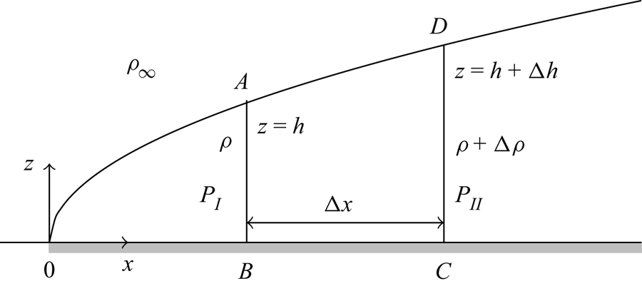
Figure 6. Schematic of the control volume  $ABCD$ and associated quantities considered in deriving (A16). At section $AB, A$ has elevation $z=h$, the pressure $P=P_{I}$ and the density is $\rho$. At section $CD, D$ has elevation $z=h+{\rm \Delta} h$, the pressure $P=P_{II}$ and the density is $\rho +{\rm \Delta} \rho$.
A.3. Conservation of energy
Following the method of Rooney & Linden (Reference Rooney and Linden1996), starting from the internal energy equation for a system capable of expansion work only and assuming an ideal gas gives
 \begin{equation} \frac{c_p}{R}\int_{\tau_p} P \boldsymbol{\nabla}\boldsymbol{\cdot}\boldsymbol{v} \, \mathrm{d}\tau = \dot{Q} - \frac{c_p}{R}\int_{\tau_p}\boldsymbol{v}\boldsymbol{\cdot}\boldsymbol{\nabla} P \, \mathrm{d}\tau, \end{equation}
where  $\tau _p$ is the volume enclosed by the plume, $\boldsymbol {v}$ is the velocity vector, $\dot {Q}$ is the total heating power input to the system and $R$ is the gas constant. For the two-dimensional geometry considered, (A17) becomes
 \begin{equation} \frac{c_p}{R}\int_{\tau_p} P \left(\frac{\partial u}{\partial x} + \frac{\partial w}{\partial z}\right) \,\mathrm{d}\tau = \dot{Q} - \frac{c_p}{R}\int_{\tau_p}\left(u\frac{\partial P}{\partial x} + w\frac{\partial P}{\partial z}\right) \,\mathrm{d}\tau. \end{equation}
Differentiating with respect to  $x$ and rearranging yields
 \begin{equation} q = \frac{\mathrm{d}\dot{Q}}{\mathrm{d} x} = \frac{c_p}{R}\int_0^h \frac{\partial}{\partial x}(uP) \,\mathrm{d}z + \frac{c_p}{R}\int_0^h \frac{\partial}{\partial z}(wP) \,\mathrm{d}z. \end{equation}
Assuming an ideal gas so that  $P = \rho R T$, where $T$ is the plume temperature,
 \begin{equation} q = \frac{\partial}{\partial x}\int_0^h (c_p \rho u T ) \,\mathrm{d}z + c_p\rho_\infty w_eT_\infty, \end{equation}
where  $T_\infty$ is the ambient temperature. Assuming a top-hat profile for $T$ (consistent with that for $\rho$) gives
 \begin{equation} \frac{q}{c_p\rho_\infty T_\infty} = \frac{\mathrm{d}}{\mathrm{d} x}\left[\frac{\rho u h T}{\rho_\infty T_\infty}\right] + w_e. \end{equation}
Taking the Boussinesq approximation yields
 \begin{equation} \frac{\mathrm{d}}{\mathrm{d} x}[uh] = \alpha_v u + \frac{q}{c_pT_\infty\rho_\infty}, \end{equation}
on taking  $w_e = - \alpha _v u$. Combining (A22) with (A4) and multiplying by $g$ gives
 \begin{equation} \frac{\mathrm{d}}{\mathrm{d} x}[g'uh] = \frac{g}{c_pT_\infty\rho_\infty}q, \end{equation}
the statement of conservation of buoyancy in (2.1c).
Appendix B. Experimental data
Table 1. Shadowgraph experiment data (to 3 significant figures), plotted in figure 4. The standard error of the mean is defined by  ${SEM} = \sigma /\sqrt {N}$ where $\sigma$ is the standard deviation and $N$ is the number of observations of the plate temperature.


 Open access