


1. Introduction
Parallel application of a pressure-driven flow and electric field can drive a net migration of long DNA strands to the walls of a capillary, and reversing the relative directions of the flow and electric field causes the DNA strands to migrate towards the centre of the capillary (Zheng & Yeung Reference Zheng and Yeung2002, Reference Zheng and Yeung2003; Arca, Butler & Ladd Reference Arca, Butler and Ladd2015). This transverse migration has been used to trap and concentrate DNA within a microfluidic chip of simple design, and evidence suggests that the process can separate DNA from other macromolecules and particulates (Arca, Ladd & Butler Reference Arca, Ladd and Butler2016; Montes, Butler & Ladd Reference Montes, Butler and Ladd2019a; Valley et al. Reference Valley, Crowell, Butler and Ladd2020).
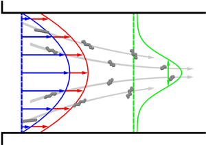
The transverse migration of DNA strands has been attributed to intramolecular velocity disturbances caused by the electric field acting on the charged backbone of the polyelectrolyte and its surrounding counterion cloud (Butler et al. Reference Butler, Usta, Kekre and Ladd2007; Usta, Butler & Ladd Reference Usta, Butler and Ladd2007; Kekre, Butler & Ladd Reference Kekre, Butler and Ladd2010b; Pandey & Underhill Reference Pandey and Underhill2015; Ladd Reference Ladd2018). These electrohydrodynamic interactions are commonly ignored when calculating the electrophoretic motion of DNA and other polyelectrolytes. However, these interactions can alter the motion if the electric double layer is large in comparison with the backbone cross-section and the DNA molecule is distorted from its equilibrium (roughly spherical) configuration. In the case of migration during a pressure-driven flow, hydrodynamic forces stretch the DNA molecule within the extensional quadrants of the local shear flow. Then, the electric field and resulting electrohydrodynamic interactions induce additional components of motion, including one transverse to the flow and field direction. When a flexible polyelectrolyte leads a pressure-driven flow upon application of an axial electric field, the transverse motion is towards the centre of the channel, as illustrated in figure 1(a); upon reversing the electric field direction, the same polyelectrolyte will lag the flow and move towards the bounding walls.

Figure 1. (a) Applying an electric field  $\boldsymbol {E}$ anti-parallel to a pressure-driven flow (blue) causes an initially uniform distribution of DNA, which is negatively charged, to lead the flow (red) and migrate towards the centre of the channel (grey field). The width of the concentration profile (green) is characterized by the standard deviation $\sigma (x)$ corresponding to the concentration profile $C(y|x)$ at position $x$. (b) Dependence of widths $\sigma ^\infty =\sigma (x \rightarrow \infty )$ of the developed concentration profiles of DNA molecules in a microfluidic channel on the electric field $E$ obtained in the experiments of Arca et al. (Reference Arca, Butler and Ladd2015) for several mean shear rates $\bar {\gamma }$ and Debye lengths $\lambda _D$. The normalization for the axes was chosen to collapse the data onto a single curve.
Two different approximations for electrohydrodynamic interactions have been employed to calculate the centre-of-mass distribution of bead–spring models of polyelectrolytes. The long-range model (Butler et al. Reference Butler, Usta, Kekre and Ladd2007; Kekre et al. Reference Kekre, Butler and Ladd2010b) treats each bead as a uniformly distributed collection of point charges, where each point charge is surrounded by counterions. The velocity disturbances caused by the electric field acting on the point charges and counterions within each bead are calculated using the algebraically decaying terms in the Green's function, while ignoring the exponentially decaying terms (Allison & Stigter Reference Allison and Stigter2000; Long & Ajdari Reference Long and Ajdari2001). The net velocity disturbance from each bead is summed pairwise over all other beads of the polymer, but velocity disturbances within the beads are ignored.
The other model assumes that the electrohydrodynamic interactions are localized to individual Kuhn steps (Liao et al. Reference Liao, Watari, Wang, Hu, Larson and Lee2010; Pandey & Underhill Reference Pandey and Underhill2015; Ladd Reference Ladd2018). This short-range approximation uses the electrophoretic mobility of rigid rods (Chen & Koch Reference Chen and Koch1996) to represent the motion of each Kuhn step. Rigid rods can move perpendicular to the electric field if the Debye length is sufficiently large and the rods are aligned at an angle with respect to the electric field. The mobility tensor relating the electric field to the motion of each bead of the polymer is obtained by averaging over the mobilities of the rods composing it. Like the long-range model, transverse motions to the flow and field are predicted only if the polyelectrolyte is distorted from its equilibrium configuration and if the electric double layer is sufficiently large with respect to the polymer backbone size.
The proposed mechanism of electrohydrodynamic migration has been validated, at least qualitatively, against experimental observations of DNA migration. For example, experiments (Arca et al. Reference Arca, Butler and Ladd2015; Montes, Ladd & Butler Reference Montes, Ladd and Butler2019b) demonstrated that migration can be eliminated by increasing the buffer salt concentration, which reduces the double-layer thickness and screens the electrohydrodynamic interactions. Some alternative mechanisms were also investigated by Montes et al. (Reference Montes, Ladd and Butler2019b) and were found to be inadequate to explain the observed migration. Additionally, experiments with anti-parallel fields (Arca et al. Reference Arca, Butler and Ladd2015) indicate that DNA initially focuses more strongly in the centre of the channel with increasing electric field, but focusing diminishes once a critical electric field is surpassed (see figure 1b). Brownian dynamics simulations using the long-range approximation predicted this increase and subsequent decline of concentration upon increasing the electric field (Kekre et al. Reference Kekre, Butler and Ladd2010b). Simulations using the short-range approximation (Pandey & Underhill Reference Pandey and Underhill2015) also predict an increase in concentration for weak fields, and more recent analysis (Setaro & Underhill Reference Setaro and Underhill2019) also suggests that the concentration declines as the electric field increases beyond a critical value.
Quantitative differences between the models and the experimental results are evident from previous studies (Kekre et al. Reference Kekre, Butler and Ladd2010b; Pandey & Underhill Reference Pandey and Underhill2015; Ladd Reference Ladd2018), but assessing the relative merits of the short- and long-range approximations is difficult due to the different parameters used. Here we report a mean-field model for a polyelectrolyte in a pressure-driven flow and an electric field which causes the polyelectrolyte to lead the flow, and hence migrate towards the centre of the channel. The model is a convection–diffusion equation with diffusion tensor and convective velocities obtained from Brownian dynamics simulations in a simple shear flow, and the mean-field model is also validated using Brownian dynamics simulations in parabolic flows. Mean-field models with the short-range and long-range approximations of the electrohydrodynamic interactions were considered.
Comparing the results with the experiments of Arca et al. (Reference Arca, Butler and Ladd2015) provides a number of conclusions regarding the models. Among them, predicting the observed migration requires setting the Debye length to a value much larger than in the experiments for the long-range model, as previously determined (Ladd Reference Ladd2018). The short-range model predicts significant migration even when the Debye length is comparable to that in the experiments, but the electric field at which focusing diminishes is much larger than measured in experiments. Also, analysis demonstrates that dispersion caused by the coupling of fluctuations of the polymer configuration and electric field causes the maximum in the extent of migration. Furthermore, the experimentally observed scaling of the width  $\sigma ^\infty$ of the developed concentration profile with the mean shear rate $\bar {\gamma }$ ( $\sigma ^\infty \propto \bar {\gamma }^{-1/2}$; see figure 1b) is explained. These results and conclusions are discussed in §§ 3–5, following presentation of the relevant theoretical background and numerical methods in § 2.
2. Theoretical background and model development
2.1. Model
We consider a DNA molecule in an ambient flow field  $\boldsymbol {u}^\infty (\boldsymbol {r})$ and a uniform electric field $\boldsymbol {E}$. The molecule is modelled as a chain of $N$ beads with coordinates $\boldsymbol {r}_1$, $\boldsymbol {r}_2$, …, $\boldsymbol {r}_N$ connected by $N-1$ springs. The dynamics of the DNA beads is described by the Langevin equation:
 \begin{equation} \frac{\textrm{d}\boldsymbol{r}_i}{\textrm{d}t} = \boldsymbol{u}^\infty(\boldsymbol{r}_i) + \sum_{j=1}^N \boldsymbol{\mu}^{H}_{ij}\boldsymbol{\cdot}(\boldsymbol{F}_j^C + \boldsymbol{F}_j^B) + \mu_0^E \boldsymbol{E} + \boldsymbol{v}_i^E. \end{equation}
Here,  $\boldsymbol {F}_i^C$ and $\boldsymbol {F}_i^B$ are the conservative and Brownian forces acting on bead $i$,
$i$,  $\boldsymbol {\mu }^{H}_{ij}$ is the mobility tensor which includes hydrodynamic interactions, $\mu _0^E$ is the electrophoretic mobility in the absence of shear and $\boldsymbol {v}_i^E$ is the velocity disturbance due to electrohydrodynamic interactions.
The conservative force includes the spring force  $\boldsymbol {F}_i^S$, the bead–bead repulsion force $\boldsymbol {F}_i^R$ and the bead–wall repulsion force $\boldsymbol {F}_i^W$:
 \begin{equation} \boldsymbol{F}_i^C = \boldsymbol{F}_i^S + \boldsymbol{F}_i^R + \boldsymbol{F}_i^W. \end{equation}
The springs connecting the beads represent freely jointed chains of  $N_K$ Kuhn steps of length $l_K$, with the tension approximated by the finitely extensible nonlinear elastic (FENE) force (Warner Reference Warner1972):
 \begin{equation} \boldsymbol{F}_i^S ={-}\sum_j\frac{\kappa\boldsymbol{r}_{ij}}{1-(r_{ij}/r_0)^2}. \end{equation}
Here, the summation is performed over beads  $j = i\pm 1$ connected to bead $i$,
$i$,  $\boldsymbol {r}_{ij}=\boldsymbol {r}_{i}-\boldsymbol {r}_{j}$ is the vector connecting beads $j$ and $i$,
$i$,  $r_{ij}$ is the magnitude of $\boldsymbol {r}_{ij}$, $\kappa = 3k_BT/l_K r_0$ is the spring constant, $k_B$ is the Boltzmann constant, $T$ is the temperature and $r_0 = N_K l_K$ is the maximum spring extension.
Excluded volume between beads is enforced using a repulsive force with potential (Kekre, Butler & Ladd Reference Kekre, Butler and Ladd2010a)
 \begin{equation} \varPhi^R(r_{ij}) = A \exp(-\beta r_{ij}^2), \end{equation}
where parameters  $A$ and $\beta$ specify the force magnitude and range. Simulations of polymers in pressure-driven flows also include a repulsive force to prevent polymer beads from passing through the channel walls. The potential energy of interaction between each bead $i$ and the bounding walls is
 \begin{equation} \varPhi^W(d_{ij}) = 2 A \exp(-\beta (d_{ij}-a)^2), \end{equation}
where  $a$ is the bead radius and $d_{ij}$ is the distance between the bead centre and wall $j$.
$j$.
Brownian forces acting on the polymer beads satisfy the fluctuation–dissipation theorem:
 \begin{equation} \left. \begin{gathered} \langle \boldsymbol{F}^B(t) \rangle = 0, \\ \langle \boldsymbol{F}^B(t)\boldsymbol{F}^B(t+\tau) \rangle = 2 k_BT (\boldsymbol{\mu}^{H})^{{-}1} \delta(\tau), \end{gathered} \right\} \end{equation}
where  $\boldsymbol {F}^B = (\boldsymbol {F}^B_1, \boldsymbol {F}^B_2, \ldots , \boldsymbol {F}^B_N)$ is the $3N$-dimensional vector containing Brownian forces acting on all of the beads, $\boldsymbol {\mu }^{H}$ is the $3N\times 3N$ grand mobility tensor and $\delta$ is the Dirac delta function.
The Rotne–Prager tensor is used to describe the hydrodynamic interactions between individual beads (Rotne & Prager Reference Rotne and Prager1969):
 \begin{equation} \boldsymbol{\mu}^{H}_{ij}(\boldsymbol{r}_{ij}) = \frac{1}{\zeta}\left\{ \begin{array}{@{}ll} \boldsymbol{\mathsf{I}}, & i=j, \\ C_1(r_{ij})\boldsymbol{\mathsf{I}} + C_2(r_{ij})\hat{\boldsymbol{r}}_{ij}\hat{\boldsymbol{r}}_{ij}, & i\ne j, \end{array}\right. \end{equation}
where  $\zeta =6{\rm \pi} \eta a$ is the drag coefficient, $\eta$ is the fluid viscosity, $\hat {\boldsymbol {r}}_{ij} = \boldsymbol {r}_{ij}/r_{ij}$ is the unit vector pointing from bead $j$ to bead $i$ and
 \begin{equation} C_1(r_{ij}) = \left\{\begin{array}{@{}ll} \displaystyle\dfrac{3a}{4r_{ij}} + \displaystyle\dfrac{a^3}{2r_{ij}^3}, & r_{ij} \ge 2a, \\ 1 - \displaystyle\dfrac{9r_{ij}}{32a}, & r_{ij} < 2a, \end{array} \right.\quad C_2(r_{ij}) = \left\{\begin{array}{@{}ll} \displaystyle\dfrac{3a}{4r_{ij}} - \displaystyle\dfrac{3a^3}{2r_{ij}^3}, & r_{ij} \ge 2a, \\ \displaystyle\dfrac{3r_{ij}}{32a}, & r_{ij} < 2a. \end{array} \right. \end{equation}
Hydrodynamic interactions between beads and walls were neglected. Kekre et al. (Reference Kekre, Butler and Ladd2010b) demonstrated that these interactions have a negligible effect on the developed concentration profile for the case studied here, where the channel dimension is much larger than the polyelectrolyte and the polyelectrolyte migrates towards the centre of the channel.
2.2. Models of electrohydrodynamic interaction
Two alternative approaches to modelling electrohydrodynamic interactions ( $\boldsymbol {v}^E_i$) were investigated. The long-range model (Butler et al. Reference Butler, Usta, Kekre and Ladd2007; Kekre et al. Reference Kekre, Butler and Ladd2010b) assumes that each bead of the polymer model represents a blob of uniformly distributed charges and utilizes the Green's function for the velocity field caused by an electric field acting on a point charge and its surrounding counterion cloud (Allison & Stigter Reference Allison and Stigter2000; Long & Ajdari Reference Long and Ajdari2001). The short-range model (Liao et al. Reference Liao, Watari, Wang, Hu, Larson and Lee2010; Pandey & Underhill Reference Pandey and Underhill2015; Ladd Reference Ladd2018) approximates electrohydrodynamic mobilities of each polymer bead by averaging the mobilities of Kuhn steps comprising the bead. The motion due to the electric field of each Kuhn step is approximated as that of a charged rigid rod (Chen & Koch Reference Chen and Koch1996) and electrohydrodynamic interactions between the Kuhn steps are neglected.
As shown in appendix A, the velocity  $\boldsymbol {v}^E_i$ of each bead $i$ can be written as
 \begin{equation} \boldsymbol{v}^E_i = \mathcal{E}_m \sum_{j\ne i}\hat{\mu}_{m,ij}^E(r_{ij})\boldsymbol{\mathsf{A}}(\hat{\boldsymbol{r}}_{ij}) \boldsymbol{\cdot} \boldsymbol{\hat{E}}, \end{equation}
where the subscript  $m$ indicates the model ( $m = L$ for long-range model and $m = S$ for short-range model) and $\boldsymbol {\hat {E}} = \boldsymbol {E}/E$ is the unit vector parallel to the electric field. The parameter $\mathcal {E}_m$ characterizes the strength of the electrohydrodynamic interactions, while $\hat {\mu }_{m,ij}^E(r)$ describes the dependence of the electrohydrodynamic interactions between beads $i$ and $j$ on the distance $r$ between them. The tensor
 \begin{equation} \boldsymbol{\mathsf{A}}(\hat{\boldsymbol{r}}_{ij}) = 3\hat{\boldsymbol{r}}_{ij}\hat{\boldsymbol{r}}_{ij} - \boldsymbol{\mathsf{I}} \end{equation}
is zero on average when the distribution of beads is isotropic, i.e.  $\langle \hat {\boldsymbol {r}}_{ij}\hat {\boldsymbol {r}}_{ij}\rangle = \boldsymbol{\mathsf{I}}/3$. This condition is met in the absence of shear, and on average the electrohydrodynamic interactions between different beads cancel out. Consequently no net migration occurs perpendicular to the electric field in this case, as expected.
For the long-range model, the summation in (2.9) is performed over all  $j\ne i$, and the model-dependent parameters in the equations are given by
 \begin{equation} \hat{\mu}_{L,ij}^E(r) = \left\{\begin{array}{@{}ll} r^{{-}3}, & r\ge 2a, \\ 0, & r < 2a \end{array}\right. \end{equation}
and
 \begin{equation} \mathcal{E}_{L} = \displaystyle\frac{3a\lambda_D^2QE}{2\zeta}. \end{equation}
Here,  $Q$ is the charge of a bead and $\lambda _D$ is the Debye length. For the short-range model, the summation on the right-hand side of (2.9) is performed only over beads $j=i\pm 1$ connected to bead $i$. The parameters in this case are given by
 \begin{equation} \hat{\mu}_{S,i,i\pm1}^E(r) = \frac{2}{N_s(i)}\frac{(r/r_0)^2}{3-(r/r_0)^2}, \end{equation}
where
 \begin{equation} N_s(i) = \left\{\begin{array}{@{}ll} 1, & i = 1\ \mathrm{or}\ i = N, \\ 2, & \mathrm{otherwise}, \end{array}\right. \end{equation}
and
 \begin{equation} \mathcal{E}_{S} = \frac{1-\alpha_\mu}{1+2\alpha_\mu}\mu_0^EE. \end{equation}
Here,  $N_s(i)$ is the number of springs connected to the $i$th bead and $\alpha _\mu = \mu _{\perp }^{E,rod}/\mu _{\parallel }^{E,rod}$ is the ratio of the Kuhn step (rod) mobility in the directions perpendicular and parallel to the rod axis. The value of $\alpha _\mu$ varies between 1/2 and 1, depending on the Debye length $\lambda _D$. According to the slender-body model for a cylinder (Chen & Koch Reference Chen and Koch1996), $\alpha _\mu \approx 1/2$ for the range of $\lambda _D$ considered in the experiment of Arca et al. (Reference Arca, Butler and Ladd2015) ( $d < \lambda _D < l_K$, where $d$ is the diameter of the rod). For a thin double layer ( $\lambda _D \ll d$), the model for an infinitely long cylinder (Ohshima Reference Ohshima1996) yields $\alpha _\mu \approx 1$ and $\mathcal {E}_{S} = 0$. No net migration occurs perpendicular to the electric field in this limit.
2.3. Model parameters
Here,  $\lambda$-DNA molecules are modelled by a chain consisting of 20 beads to facilitate comparison with experiments. Each subchain connecting neighbouring beads corresponds to $N_K = 10$ Kuhn steps of length $l_K = 106\ \textrm {nm}$ each. The corresponding bead charge obtained from the Manning condensation model (Manning Reference Manning1969) is $Q = 1493.6e$. Throughout this work, parameter values are normalized using the characteristic length $b = \sqrt {k_BT/\kappa } = l_K\sqrt {N_K/3}= 193.5\ \textrm {nm}$, characteristic time $t_c = \zeta /\kappa = 0.0122\ \textrm {s}$, characteristic energy $k_BT$ and elementary charge $e$. With this choice of characteristic values, the dimensionless values of the spring constant $\kappa$ and the drag coefficient $\zeta$ both equal one. Dimensionless values of other model parameters that are kept constant throughout this work are summarized in table 1. These values match those used by Kekre et al. (Reference Kekre, Butler and Ladd2010a,b), with the exception of the electrophoretic mobility $\mu _0^E$. The value of $\mu _0^E= 120.7$ measured in experiments (Montes Reference Montes2018) for a buffer with an estimated Debye length $\lambda _D = 0.03$ was used (see § S1 of the supplementary material available at https://doi.org/10.1017/jfm.2021.11).
Table 1. Dimensionless values of the parameters of the  $\lambda$-DNA model that are kept constant throughout this work.

Additional parameters that characterize the strength of the electrohydrodynamic interactions, such as the Debye length  $\lambda _D$ for the long-range model and the ratio $\alpha _\mu$ for the short-range model, are absorbed into the parameters $\mathcal {E}_{L}$ and $\mathcal {E}_{S}$, respectively. These latter parameters are varied systematically in the computations.
It should be noted that the parameters  $\mathcal {E}_{L}$ and $\mathcal {E}_{S}$ corresponding to the same electric field strength $E$ differ by three orders of magnitude for typical experimental conditions, $\alpha _\mu \approx 1/2$, $\lambda _D = O(10^{-2})$. For these conditions, (2.12) and (2.14) yield
 \begin{equation} \frac{\mathcal{E}_{L}}{\mathcal{E}_{S}} \approx \displaystyle\frac{6a\lambda_D^2Q}{\mu_0^E} = O(10^{{-}3}). \end{equation}
2.4. Brownian dynamics simulations
Simulations of the Langevin equation (2.1) were performed using the Brownian dynamics method (Ermak & McCammon Reference Ermak and McCammon1978). Three different flow fields  $\boldsymbol {u}^\infty (\boldsymbol {r})$ were investigated, namely pressure-driven flows in two different geometries and a simple shear flow. In all simulations, the flow and electric field were directed along the $x$ axis, which causes the polyelectrolyte to lead the flow since $\mu _0^E>0$. As a result, transverse migration occurs from regions of high flow rate to regions of low flow rate.
Initial configurations of the bead positions were sampled from simulations in the absence of a flow and electric field, where these equilibrium simulations were long compared to the correlation time of 42 for the end-to-end vector (see § S2 of the supplementary material). Time steps between  $10^{-4}$ and $10^{-3}$ were used, depending on the shear rate and the strength of the electric field, with stronger rates and fields requiring smaller time steps. The step-size selection was validated by confirming that the structural and transport properties of polymers were consistent with those obtained with simulations using smaller step sizes.
The considered pressure-driven flows were flows between parallel plates separated by a distance  $H$ (referred to as the two-dimensional or 2-D flow) and through a channel of cross-section $H \times H$ (referred to as the three-dimensional or 3-D flow). The dimension of $H=413$ was chosen to match the experiments of Arca et al. (Reference Arca, Butler and Ladd2015), and the flow is characterized by the mean shear rate $\bar {\gamma } = 2v_0/H$, where $v_0$ is the centreline flow velocity. For flows through a square cross-section, $\boldsymbol {u}^\infty (\boldsymbol {r})$ was determined numerically using a finite-difference solution of the Stokes equation for a unidirectional flow and $\boldsymbol {u}^\infty (\boldsymbol {r}_i)$ for each bead was obtained by the bilinear interpolation of the numerically obtained velocity values stored on a square grid.
For each set of conditions (flow and electric fields, geometry), a total of  $10^4$ bead–spring chains were initially distributed at the entry ( $x=0$) and simulated for a channel length sufficient to attain a fully developed concentration profile. Concentration profiles $C(\boldsymbol {\rho }|x)$ at various positions $x$ along the channel were computed ( $\boldsymbol {\rho }$ represents the transversal coordinates of the polymer centre of mass, $\boldsymbol {\rho } = y$ for 2-D flows and $\boldsymbol {\rho } = (y,z)$ for 3-D flows). The width of the concentration profile in the 2-D channel is characterized by the standard deviation $\sigma (x)$ corresponding to the concentration profile $C(y|x)$ at position $x$. To obtain the width of the concentration profile in the 3-D channel, the concentration $C(y,z|x)$ was first averaged in the depth ( $z$ direction) to obtain a 2-D profile $C_{av}(y|x)$. This was followed by computing the standard deviation $\sigma (x)$ of $C_{av}(y|x)$. This approach was chosen over a more straightforward calculation of the standard deviation of the 3-D concentration profile $C(y,z|x)$ to mimic experimental measurements of Arca et al. (Reference Arca, Butler and Ladd2015).
For simple shear flow, at least 2000 trajectories were simulated for each set of parameter values (shear rate and electric field). Each trajectory was simulated for a duration of  $5000$, but only data for times greater that $500$ were used in the analysis. The mean polymer velocity $\boldsymbol {V}_c$ was obtained by fitting the ensemble average of the polymer displacement from its initial equilibrated position to a straight line, $\langle \boldsymbol {R}_c(t)\rangle = \boldsymbol {V}_ct$. The diffusion tensor was obtained from deviations $\boldsymbol {\xi }_c(t) \equiv \boldsymbol {R}_c(t) - \boldsymbol {V}_c t$ of individual trajectories from the mean trajectory by fitting each of the components of the mean-squared displacement tensor $\langle \boldsymbol {\xi }_c(t)\boldsymbol {\xi }_c(t)\rangle$ to a straight line. Both $\langle \boldsymbol {R}_c(t)\rangle$ and $\langle \boldsymbol {\xi }_c(t)\boldsymbol {\xi }_c(t)\rangle$ increase linearly in time (see § S3.1 of the supplementary material), and consequently the motion of the polymer centre of mass can be modelled by a Langevin equation, as described next.
2.5. Mean-field model
Results from Brownian dynamics simulations of polyelectrolytes in simple shear flows were used to develop a mean-field model for the polymer distribution in more complex geometries. The model assumes that motion of the polymer centre of mass  $\boldsymbol {R}_c$ can be described by the following Langevin equation:
 \begin{equation} \dot{\boldsymbol{R}}_c(t) = \boldsymbol{u}^\infty(\boldsymbol{R}_c) + \mu_0^E\boldsymbol{E} + \boldsymbol{V}_c + \boldsymbol{\varGamma}_c(t), \end{equation}
where  $\boldsymbol {V}_c$ is the mean contribution of the electrohydrodynamic interactions to the velocity of the centre of mass and $\boldsymbol {\varGamma }_c$ is the effective random force acting on the centre of mass. Here $\boldsymbol {\varGamma }_c$ contains contributions from the Brownian force and the fluctuating component of the electrohydrodynamic interactions caused by fluctuations of the polymer configuration. The random force $\boldsymbol {\varGamma }_c$ has a zero mean and covariance
 \begin{equation} \langle\boldsymbol{\varGamma}_c(t)\boldsymbol{\varGamma}_c(t+\tau)\rangle = 2\boldsymbol{\mathsf{D}} \delta(\tau), \end{equation}
where  $\boldsymbol{\mathsf{D}}$ is the effective diffusion tensor.
Therefore, the polymer concentration  $C(\boldsymbol {r})$ is expected to obey a convection–diffusion equation with position-dependent drift velocity and diffusivity:
 \begin{equation} \frac{\partial C}{\partial t} = \boldsymbol{\nabla}\boldsymbol{\cdot}[\boldsymbol{\mathsf{D}}\boldsymbol{\nabla} - (\boldsymbol{u}^\infty + \mu_0^E\boldsymbol{E} + \boldsymbol{V}_c)]C. \end{equation}
In a simple shear flow, statistics of the polymer configuration are independent of the polymer position and, hence,  $\boldsymbol {V}_c$ and $\boldsymbol{\mathsf{D}}$ are constant. In a more complex flow geometry, $\boldsymbol {V}_c$ and $\boldsymbol{\mathsf{D}}$ are position-dependent, with their value determined by the local shear $\gamma (\boldsymbol {r})$. The model (2.18) is valid if the memory effects can be neglected, i.e. the polymer instantly acquires its diffusivity and velocity corresponding to the local environment. This assumption holds since the response time of the polymer to changes in the environment is much smaller than the time it takes the polymer to move from one streamline to another. This is verified by the Brownian dynamics simulations discussed in § 3 and the time-scale analysis presented in § S4.3.1 of the supplementary material.
The mean-field model is applied to pressure-driven unidirectional flows in the same 2-D and 3-D geometries as those considered in the Brownian dynamics simulations. In these systems, the local shear rate  $\gamma (\boldsymbol {r})$ depends only on the transverse coordinates $\boldsymbol {\rho }$ and is independent of the position $x$ along the channel length. Hence, the local drift velocity and diffusivity are also independent of $x$. Moreover, transport in the $x$ direction is dominated by the convective and electrophoretic velocities and the diffusivity in the $x$ direction can be neglected (see § S4.3.2 of the supplementary material). Assuming furthermore that the system is at steady state, (2.18) can be approximated as
 \begin{equation} (u^\infty_x(\boldsymbol{\rho}) + \mu_0^E E + V_{c,x}(\boldsymbol{\rho})) \frac{\partial C(x,\boldsymbol{\rho})}{\partial x} = L_{\boldsymbol{\rho}} C(x,\boldsymbol{\rho}), \end{equation}
where
 \begin{equation} L_{\boldsymbol{\rho}} = \boldsymbol{\nabla}_{\boldsymbol{\rho}}\boldsymbol{\cdot}(\boldsymbol{\mathsf{D}}_{\boldsymbol{\rho}}\boldsymbol{\nabla}_{\boldsymbol{\rho}} - \boldsymbol{V}_{c,\boldsymbol{\rho}}) \end{equation}
is the convection–diffusion operator in the transverse directions. The diffusion tensor  $\boldsymbol{\mathsf{D}}_{\boldsymbol {\rho }}$ and the mean velocity $\boldsymbol {V}_{c,\boldsymbol {\rho }}$ in (2.20) contain only the elements corresponding to the transverse motion, i.e. for the 2-D flows, $\boldsymbol {V}_{c,\boldsymbol {\rho }} = V_{c,y}$, $\boldsymbol{\mathsf{D}}_{\boldsymbol {\rho }} = D_{yy}$ and for the 3-D flows,
 \begin{equation} \boldsymbol{V}_{c,\boldsymbol{\rho}} = \left[\begin{array}{@{}c@{}} V_{c,y} \\ V_{c,z} \end{array} \right], \quad \boldsymbol{\mathsf{D}}_{\boldsymbol{\rho}} = \left[\begin{array}{@{}cc@{}} D_{yy} & D_{yz} \\ D_{yz} & D_{zz} \end{array} \right]. \end{equation}
 The values of  $\boldsymbol {V}_c$ and $\boldsymbol{\mathsf{D}}$ were obtained from a series of Brownian dynamics simulations in a simple shear flow, which yield dependence of $\boldsymbol {V}_c$ and $\boldsymbol{\mathsf{D}}$ on $\gamma$. To utilize these quantities in the mean-field model for a pressure-driven flow, the local shear $\gamma (\boldsymbol {\rho })$ in the flow is computed and spline interpolation of $\boldsymbol {V}_c(\gamma )$ and $\boldsymbol{\mathsf{D}}(\gamma )$ is performed to obtain their values corresponding to $\gamma (\boldsymbol {\rho })$. This yields velocities and diffusivities in a local system of coordinates $x\eta \zeta$ with the $\eta$ and $\zeta$ axes pointing in the directions of $(0, \partial _y u^\infty _x, \partial _z u^\infty _x)$ and $(0, -\partial _z u^\infty _x, \partial _y u^\infty _x)$, respectively. The tensor $\boldsymbol{\mathsf{D}}$ and the vector $\boldsymbol {V}_c$ are then rotated to obtain the diffusivity and the velocity in the directions of $x$,
$x$,  $y$ and $z$.
$z$.
Equation (2.19) was solved numerically using a finite-difference approximation for the operator  $L_{\boldsymbol {\rho }}$ and the Runge–Kutta method for integration in the $x$ direction. In addition, the developed profiles (corresponding to $\partial C/\partial x = 0$) were obtained directly by solving (2.19) with zero left-hand side. In the 2-D channel, this equation is solved analytically (see appendix B). In the 3-D channel, the developed profiles were obtained by numerically computing the eigenfunction corresponding to the zero eigenvalue of the operator $L_{\boldsymbol {\rho }}$.
3. Results
Results of Brownian dynamics simulations in a simple shear flow are presented in §§ 3.1 and 3.2, with comparisons between the long-range and short-range models for the electrohydrodynamic interactions. Then, results for pressure-driven flows are given in § 3.3, which include results of Brownian dynamics simulations and mean-field calculations. The shear rate is reported in terms of the Peclet number, i.e. dimensionless  $\gamma$. Note that the Weissenberg number is given by $12\gamma$ (see § S2 of the supplementary material).
3.1. Mean velocity in simple shear flow
Dependence of the transverse velocity  $V_{c,y}(\gamma ,\mathcal {E}_m)$ of the polymer centre of mass in the simple shear flow on the shear rate $\gamma$ is shown in figure 2 for several values of the electric field strength $\mathcal {E}_m$. Drift in the transverse direction is caused solely by electrohydrodynamic interactions. At zero shear rate, the polymer shape is nearly isotropic and the electrohydrodynamic interactions between polymer beads cancel out (see the discussion following (2.10)). Hence, $V_{c,y}(\gamma = 0; \mathcal {E}_m) = 0$ for all $\mathcal {E}_m$. Application of shear stretches and tilts the polymer with respect to the field direction, resulting in a non-zero electrohydrodynamic velocity $V_{c,y}$ in the transverse direction.

Figure 2. Mean transverse velocity  $V_{c,y}$ in simple shear flows with rate $\gamma$. The results were obtained from Brownian dynamics simulations using (a) long-range and (b) short-range models for the electrohydrodynamic interactions. The velocities are normalized by the strength of the electric field $\mathcal {E}_m$ to facilitate discussion of the effects of $\mathcal {E}_m$ on $V_{c,y}$.
The long- and short-range electrohydrodynamic models predict qualitatively different dependence of  $V_{c,y}$ on $\gamma$. The long-range model yields a non-monotonic dependence of $V_{c,y}$ on $\gamma$ (see figure 2a): $V_{c,y}$ increases with $\gamma$ for sufficiently small $\gamma$ and decreases with further increase of $\gamma$, where both the maximum value and shear rate at which it occurs are functions of $\mathcal {E}_{L}$. In contrast, the short-range model predicts a monotonic increase of $V_{c,y}$ with $\gamma$ (see figure 2b).
The qualitative differences observed in figure 2 cannot be attributed to changes in the structural properties of the polymer arising from the choice of electrohydrodynamic model. As shown in figure 3, the electrohydrodynamic model alters the structure quantitatively, but not qualitatively. Instead, the differences in  $V_{c,y}$ arise from the dependencies of the electrohydrodynamic interactions on polymer stretching. As the polymer end-to-end distance increases in response to larger shear rates (see figure 3a,b), the magnitude of the electrohydrodynamic interactions can decrease or increase depending on which model is used.

Figure 3. Structural properties of the polymer in a simple shear flow obtained from Brownian dynamics simulations. The root-mean-squared end-to-end distance  $\langle R^2 \rangle ^{1/2}$ is shown for the (a) long- and (b) short-range electrohydrodynamic models. The normalized covariance $\varSigma _{xy} = \langle R_x R_y\rangle /\langle R^2 \rangle$ of the $x$ and $y$ components of the end-to-end vector $\boldsymbol {R}$ are also shown for the (c) long- and (d) short-range models. Data are shown as a function of shear rate $\gamma$ and electric field $\mathcal {E}_m$.
Within the long-range model,  $\hat {\mu }_{L,ij}^E(r)$ decreases as the distance $r$ between beads increases (see (2.11)). This is consistent with the behaviour of $V_{c,y}$ obtained with the long-range model at high shear rates. The behaviour of $V_{c,y}$ at low shear rates is explained by the effect of the bond direction on electrohydrodynamic interactions. It follows from (2.9) and (2.10) that the velocity in the $y$ direction induced by an electric field applied in the $x$ direction is proportional to $\hat {r}_x\hat {r}_y$, where $\hat {\boldsymbol {r}}$ is the normalized vector connecting pairs of polymer beads. On average, $\hat {r}_x\hat {r}_y$ can be characterized by the normalized covariance between the $x$ and $y$ components of the end-to-end vector $\boldsymbol {R}$ of the polymer, $\varSigma _{xy} = \langle R_x R_y\rangle /\langle R^2 \rangle$. This covariance, shown in figure 3(c,d), exhibits a non-monotonic dependence on $\gamma$. Therefore, at low shear rates, the decreasing trend of $\hat {\mu }_{L,ij}^E(r)$ competes with a very rapid increase of $\varSigma _{xy}$. Thus, $V_{c,y}$ obtained with the long-range model increases with $\gamma$ at low shear rates.
Within the short-range model,  $\hat {\mu }_{S,i,i\pm 1}^E(r)$ increases as the distance $r$ between beads increases (see (2.13a)), which is consistent with the observed dependence of $V_{c,y}$ on the shear rate (see figure 2b). At large $\gamma$, there is a competition between decreasing $\varSigma _{xy}$ and increasing $\hat {\mu }_{S,i,i\pm 1}^E(r)$. For the range of $\gamma$ considered in the current work, the increase of $\hat {\mu }_{S,i,i\pm 1}^E(r)$ is more substantial than the decrease of $\varSigma _{xy}$ and, hence, the magnitude of $V_{c,y}$ grows with $\gamma$. The theoretical prediction of Ladd (Reference Ladd2018) (which neglected the effect of the electrohydrodynamic interactions on the polymer configuration) shows that $V_{c,y}$ eventually reaches a maximum at large $\gamma$. However, this maximum is observed at a very high shear rate ( $\gamma > 4$ in the current normalization), which is well beyond the values considered in the current simulations and the experiments of Arca et al. (Reference Arca, Butler and Ladd2015). Moreover, this maximum is very weak, i.e. the rate of decrease of $V_{c,y}$ beyond this maximum is very small.
Figure 2 indicates that the transverse velocity depends on the field strength  $\mathcal {E}_m$ as well as the shear rate. Since the magnitude of the instantaneous electrohydrodynamic velocity $\boldsymbol {v}_i^E$ of a bead is directly proportional to $\mathcal {E}_m$, it is expected that $V_{c,y}$ is also proportional to $\mathcal {E}_m$. This is indeed the case for the short-range model, as evident from figure 2(b). However, this is not always the case for the long-range model. The discrepancy is caused by changes in the polymer configuration induced by the electric field. For example, figure 3 shows that the root-mean-squared end-to-end distance $\langle R^2\rangle ^{1/2}$ and the normalized covariance $\varSigma _{xy}$ of the end-to-end vector are affected by $\mathcal {E}_m$. Although the electric field also affects the polymer shape in the short-range model, its effect on $V_{c,y}$ is not as significant as in the long-range model. Despite the deviation from the linear dependence of $V_{c,y}$ on $\mathcal {E}_m$ in the long-range model, $V_{c,y}$ can be approximated by a power-law dependence on $\mathcal {E}_m$:
 \begin{equation} V_{c,y}(\gamma,\mathcal{E}_m) = \hat{V}_{c,y}(\gamma) \mathcal{E}_m^{p(\gamma)} \end{equation}
(see figure S4 in the supplementary material), with the exponent  $p(\gamma )$ close to one. Dependence of the power-law exponent $p(\gamma )$ on the shear rate is shown in figure 4.

Figure 4. Power-law exponents  $p$ and $q$ for the empirical relationships (3.1) and (3.2) describing the effect of the strength of the electric field $\mathcal {E}_m$ on the velocity $V_{c,y}$ and the diffusivity $D_{yy}$ in the transverse direction predicted by the long-range (LR) and short-range (SR) electrohydrodynamic models.
In addition to the qualitative difference in the mean drift velocities  $V_{c,y}$, the long- and short-range models yield a substantial quantitative difference. Since the magnitudes of the parameters $\mathcal {E}_{L}$ and $\mathcal {E}_{S}$ corresponding to the same electric field strength $E$ differ by three orders of magnitude for typical experimental conditions (see (2.15)) and the magnitudes of the normalized velocities $V_{c,y}/\mathcal {E}_m$ ( $m = L$ or $S$) predicted by both electrohydrodynamic models are comparable (see figure 2), the values of velocities predicted by the long-range model are substantially smaller than those predicted by the short-range model at the same electric field and Debye length. To achieve the same transverse velocity at the same electric field in the long- and short-range models, it is necessary to increase the Debye length in the long-range model. This finding matches that of Ladd (Reference Ladd2018).
3.2. Diffusivity in simple shear flow
The polymer diffusivity is also sensitive to  $\mathcal {E}_m$, as shown in figure 5. This is explained by dispersion effects of electrohydrodynamic interactions: as the polymer configuration fluctuates, so do the electrohydrodynamic interactions between its beads. Therefore, in addition to the regular Brownian force due to thermal collisions between the polymer and the solvent, the random force acting on the polymer contains a contribution from the fluctuating component of electrohydrodynamic interactions. More specifically, the dynamics of internal degrees of freedom of the polymer contribute to translation of the polymer centre of mass. It is shown in § S3.3 of the supplementary material that the electrohydrodynamic dispersion is dominated by fast fluctuations of individual polymer beads. Contribution of slow fluctuations of the molecule as a whole (e.g. tumbling) is negligible in comparison with the fast fluctuations.

Figure 5. Contribution of electrohydrodynamic dispersion to polymer diffusivity in the  $y$ direction in the simple shear flow obtained from Brownian dynamics simulations using (a) long-range and (b) short-range models. The dashed lines show fits of the data to the empirical relationship (3.2).
Fluctuations of electrohydrodynamic velocity increase in magnitude as the electric field becomes stronger. If the electric field were not to alter the polymer configuration, the instantaneous electrohydrodynamic force would be proportional to the field strength  $\mathcal {E}_m$ and, hence, the contribution of this force to the diffusivity would scale as $\mathcal {E}_m^2$. However, as in the case with the mean drift velocity $V_{c,y}$, the polymer deformation caused by the electric field alters the value of the exponent. Therefore, the diffusivity is approximated by a more general expression:
 \begin{equation} D_{yy}(\gamma,\mathcal{E}_m) = D^B_{yy}(\gamma)+ D_{yy}^E(\gamma)\mathcal{E}_m^{q(\gamma)}, \end{equation}
where  $D^B_{yy}(\gamma ) = D_{yy}(\gamma ,0)$ is the diffusivity due to the Brownian force and the second term of (3.2) represents the electrohydrodynamic dispersion. The Brownian diffusivity is obtained from simulations in the absence of an electric field and the characteristics of the electrohydrodynamic dispersion, $D_{yy}^E$ and $q$, are obtained by fitting $[D_{yy}(\gamma ,\mathcal {E}_m) - D^B_{yy}(\gamma )]$ to a power law, as shown in figure 5. Dependence of the power-law exponent $q(\gamma )$ on the shear rate $\gamma$ is shown in figure 4. It is observed that $q(\gamma )> 1$ for all considered shear rates $\gamma$.
In addition to  $V_{c,y}$ and $D_{yy}$, the mean-field model for the 3-D pressure-driven flow requires $D_{zz}$ and $D_{yz}$. The component $D_{zz}$ exhibits trends qualitatively similar to those of $D_{yy}$ (see figure S5 in the supplementary material), with the power-law exponents $q$ within the same range. The component $D_{yz}$ is at least an order of magnitude smaller than $D_{yy}$ and $D_{zz}$ (see figure S3 in the supplementary material) and is therefore neglected in the mean-field analysis presented in § 3.3.
3.3. Pressure-driven flows
Brownian dynamics simulations of 2-D and 3-D pressure-driven flows were performed for a mean shear rate  $\bar {\gamma } = 0.146$, which corresponds to the largest used in the experiments of Arca et al. (Reference Arca, Butler and Ladd2015). Typical evolution of the concentration profile in the 2-D flow is shown in figure 6. It is observed that the distribution of the polyelectrolyte narrows downstream of the channel entrance at $x=0$, where the distribution was uniform. The concentration profile eventually becomes independent of the position $x$ along the channel, and this fully developed concentration profile is independent of the initial conditions as shown in figures S9–S11 in the supplementary material. Therefore, unless stated otherwise, we focus on results obtained with the initial conditions determined from the experimental data (see § S4.1 in the supplementary material) which are not quite uniform at $x=0$.

Figure 6. Concentration profiles in a 2-D pressure-driven flow at various positions  $x$ along the channel obtained by the Brownian dynamics simulations with uniform initial conditions. The results were generated using the long-range model with $\mathcal {E}_{L} = 9.41$ and $\bar {\gamma } = 0.146$. Positions $x \ge 10^5$ correspond to the fully developed profile. The profiles are normalized so that $\int C(y)\,{\textrm {d}y} = 1$.
Evolution of the concentration profile width  $\sigma$ (see figure 1a for definition) along the channel length is shown in figure 7 for 2-D flows; similar results were obtained for 3-D flows, as shown in figure S12 in the supplementary material. Results, shown for a range of electric fields with a fixed flow rate (mean shear), indicate that the distribution moves towards its developed value more rapidly with increasing electric field.

Figure 7. Dependence of widths  $\sigma$ of the concentration profiles on position $x$ along the channel in 2-D pressure-driven flows. The data were obtained by the Brownian dynamics simulations (solid lines) and the mean-field model (dashed lines) at $\bar {\gamma } = 0.146$ using (a) long-range and (b) short-range approximations. The inset in (b) shows a magnified area corresponding to developed profiles for $\mathcal {E}_{S} = 6.15$, 12.30 and 16.40.
To further facilitate analysis of pressure-driven flows, we utilize the mean-field model described in § 2.5. One of the main assumptions of this model is that the polymer adjusts to its local environment (determined by a local shear rate) much faster than it travels in the transverse direction. This enables us to use the values of the velocity  $\boldsymbol {V}_c$ and the diffusivity $\boldsymbol{\mathsf{D}}$ determined from the Brownian dynamics simulations in simple shear flows. This assumption is validated by an order-of-magnitude estimation of the relevant time scales presented in § S4.3.1 of the supplementary material. In addition, the validity of the mean-field model is confirmed by a direct comparison of its predictions with the Brownian dynamics simulations. As shown in figure 7, results of the mean-field model (shown by the dashed lines) and the Brownian dynamics (solid lines) are in excellent agreement for the 2-D pressure-driven flow; the mean-field model accurately predicts not only the developed profiles, but also the transient states. Similarly good agreement between the mean-field model and the Brownian dynamics simulations is observed for the 3-D pressure-driven flow (see figure S14 in the supplementary material). In § S4.4 of the supplementary material we utilize the mean-field model to investigate developing concentration profiles and assess effects of the electric field strength and the mean shear rate on the entrance length required to reach a developed profile. In the remainder of this section, we apply the mean-field model to analyse well-developed profiles.
Figure 7 indicates that the width  $\sigma ^\infty$ ( $\sigma$ as $x \rightarrow \infty$) of the fully developed profile is a non-monotonic function of the electric field $\mathcal {E}_m$ for both models of electrohydrodynamic interactions. This non-monotonic dependence is shown more clearly in figure 8 using data from the mean-field calculations. The difference between $\sigma ^\infty$ in the 2-D and 3-D flows is small, with the 3-D flow producing slightly wider concentration profiles than the 2-D flow at the same $\mathcal {E}_m$ and $\bar {\gamma }$. The similarity between the 2-D and 3-D flows is also observed during the development stage of the profiles (see figure S12 in the supplementary material). In particular, the rate of convergence towards a developed profile is almost the same in 2-D and 3-D geometries at identical $\mathcal {E}_m$ and $\bar {\gamma }$.

Figure 8. Widths ( $\sigma ^\infty$) of the developed profiles in 2-D and 3-D pressure-driven flows with mean shear rate $\bar {\gamma } = 0.146$ in channels of width $H = 413$ obtained using the mean-field model for the long-range (LR) and short-range (SR) approximations of the electrohydrodynamic interactions. The asterisks and crosses indicate the approximate solutions (3.9) of the 2-D mean-field model.
Since the 2-D and 3-D pressure-driven flows yield similar results, the remainder of this paper focuses on analysis of the 2-D flow. The 2-D flow velocity profile and the local shear rate corresponding to the mean shear rate of  $\bar {\gamma }$ are
 \begin{equation} u^\infty_x(y) = \frac{2\bar{\gamma}}{H}\left[\left(\frac{H}{2}\right)^2 - y^2\right] \end{equation}
and
 \begin{equation} \gamma(y) ={-}\frac{4\bar{\gamma} y}{H}, \end{equation}
respectively (the system of coordinates is chosen so that  $y = 0$ corresponds to the centre of the channel). As shown in appendix B, the developed concentration profile in a 2-D channel is
 \begin{equation} C(y;\mathcal{E}_m) \propto \exp\left[ \int_0^{y} R(\gamma(y');\mathcal{E}_m)\,{\textrm{d}y}'\right], \end{equation}
where
 \begin{equation} R(\gamma;\mathcal{E}_m) = \frac{V_{c,y}(\gamma;\mathcal{E}_m)}{D_{yy}(\gamma;\mathcal{E}_m)} \end{equation}
is the ratio of the transverse velocity and diffusivity.
The electrohydrodynamic drift vanishes in the absence of shear,  $V_{c,y}(\gamma = 0) = 0$. Therefore, to leading order,
 \begin{equation} R(\gamma;\mathcal{E}_m) \approx c(\mathcal{E}_m)\gamma \end{equation}
for small  $\gamma$. The function $c$ depends only on the type of the electrohydrodynamic model and the strength $\mathcal {E}_m$ of the electric field. Substituting (3.4) and (3.7) into (3.5), we obtain
 \begin{equation} C(y;\mathcal{E}_m) \propto \exp\left[\int_0^{y} c(\mathcal{E}_m)\gamma(y')\,{\textrm{d}y}'\right] = \exp\left[-\frac{2c(\mathcal{E}_m)\bar{\gamma}}{H}y^2\right]. \end{equation}
Hence, the developed concentration profile can be approximated by a Gaussian distribution with the standard deviation
 \begin{equation} \sigma^\infty(\bar{\gamma};\mathcal{E}_m) = \frac{1}{2}\left[\frac{H}{c(\mathcal{E}_m)\bar{\gamma}}\right]^{1/2}. \end{equation}
 As shown in figure 8, this approximation is in good agreement with the solution of the full 2-D mean-field equation (B1) for most of the considered conditions. The only exception is the profile at the lowest considered electric field strength ( $\mathcal {E}_{L} = 0.03$) in the long-range model. The discrepancy is caused by an inaccuracy of the linear approximation (3.7) inside this wide profile: the local shear rate at distance $\sigma ^\infty (\mathcal {E}_{L}=0.03)\approx 80$ from the channel centre is $\gamma \approx 0.1$. It is clear from figure 9(a) that dependence of $R(\gamma; \mathcal {E}_{L} \leq 0.31)$ deviates from the linear behaviour for $0 \le \gamma \le 0.1$, which explains the discrepancy between the approximate and full solution of the mean-field model. Note that the approximation (3.9) works much better for a concentration profile of comparable width obtained with the short-range model (at $\mathcal {E}_{S} = 0.21$). This good agreement is due to the fact that $R(\gamma; \mathcal {E}_{S} = 0.21)$ exhibits a linear dependence on $\gamma$ for a wide range of $\gamma$ (see figure 9b).

Figure 9. Ratio  $R = V_{c,y}/D_{yy}$ of the transverse velocity and diffusivity in a simple shear flow. The ratio $R$ was obtained from the Brownian dynamics simulations using (a) long-range and (b) short-range models.
4. Discussion
4.1. Dependence of the profile width on the mean shear rate
The approximate expression (3.9) for the developed profile width  $\sigma ^\infty$ indicates that $\sigma ^\infty \propto \bar {\gamma }^{-1/2}$. This scaling is consistent with the experimental observations of Arca et al. (Reference Arca, Butler and Ladd2015) (see figure 1b). This scaling was also obtained analytically for a dumbbell polyelectrolyte model with the long-range (Butler et al. Reference Butler, Usta, Kekre and Ladd2007) and short-range (Setaro & Underhill Reference Setaro and Underhill2019) approximations of the electrohydrodynamic interactions. The current work demonstrates that the scaling holds for more general multi-bead polymer models. Since the approximation (3.9) is based on the leading-order term of the Taylor series expansion of the ratio $R = V_{c,y}/D_{yy}$ (see (3.7)), the scaling $\sigma ^\infty \propto \bar {\gamma }^{-1/2}$ does not depend on details of the electrohydrodynamic model, as long as $\bar {\gamma }$ is sufficiently small.
Furthermore, this scaling may hold even at a relatively large mean shear rate  $\bar {\gamma }$, provided that the ratio of the transverse velocity and diffusivity remains proportional to the shear rate (3.7) within the fully developed flow. This condition is satisfied if the developed concentration profile is sufficiently narrow (i.e. the polymers are concentrated in the low-shear region) and/or the linear approximation (3.7) is valid for a wide range of $\gamma$. Figure 9 indicates that the latter condition is satisfied for the short-range model, whereas the long-range model exhibits a strongly nonlinear (non-monotonic) dependence of the ratio $R$ on $\gamma$. Therefore, it is expected that, within the short-range model, the $\bar {\gamma }^{-1/2}$ scaling of $\sigma ^\infty$ holds even for wide concentration profiles and large shear rates. On the other hand, the long-range model is expected to yield this scaling only for small shear rates and/or sufficiently large electric field strength (since the latter produces a strong focusing of the polyelectrolyte).
This is confirmed by figure 10, which shows  $\sigma ^\infty (\bar {\gamma })$ obtained by solving the full mean-field equation (B1) for the 2-D pressure-driven flow. For the short-range model, the scaling $\sigma ^\infty \propto \bar {\gamma }^{-1/2}$ holds even for relatively wide concentration profiles (observed at a low electric field strength). In contrast, in the long-range model, this scaling holds only for relatively narrow concentration profiles. At a weak electric field, the long-range model predicts the $\bar {\gamma }^{-1/2}$ scaling only for very small $\bar {\gamma }$. However, at a moderate electric field strength, the concentration profile is sufficiently narrow so that the $\bar {\gamma }^{-1/2}$ scaling holds at relatively large $\bar {\gamma }$ even with the long-range model.

Figure 10. Effect of the mean shear rate  $\bar {\gamma }$ on the width $\sigma ^\infty$ of the developed concentration profile in a 2-D pressure-driven flow predicted by the mean-field model for the long-range (LR) and short-range (SR) approximations of the electrohydrodynamic interactions. The dashed lines show results of a fit of $\sigma ^\infty (\bar {\gamma })$ to $\sigma _0\bar {\gamma }^{-1/2}$ ( $\sigma _0$ is a constant).
4.2. Dependence of the profile width on the electric field strength
As shown in figure 8, both the long- and short-range models predict the existence of an optimal field strength  $\mathcal {E}_m^*$ leading to the narrowest concentration profile. This is in qualitative agreement with experimental observations of Arca et al. (Reference Arca, Butler and Ladd2015) (see figure 1b), previous simulations of the long-range model (Kekre et al. Reference Kekre, Butler and Ladd2010b) and analysis of the short-range model for a dumbbell approximation to a polymer (Setaro & Underhill Reference Setaro and Underhill2019). Here, we explain the mechanism leading to existence of the optimal field strength.
Equation (3.9) indicates that the optimal field  $\mathcal {E}_m^*$ corresponds to the maximum of $c(\mathcal {E}_m)=\partial R(\gamma; \mathcal {E}_m)/\partial \gamma |_{\gamma = 0}$. Therefore, at small shear rates $\gamma$, $\mathcal {E}_m^*$ corresponds to the maximum of the ratio $R(\gamma; \mathcal {E}_m)$ of the drift velocity and diffusivity in the transverse direction. This maximum arises due to an interplay between the Brownian motion and the electrohydrodynamic drift and dispersion. To see this, consider the inverse of $R$ and use the empirical relationships (3.1) and (3.2) for $V_{c,y}$ and $D_{yy}$:
 \begin{equation} R^{{-}1}(\gamma;\mathcal{E}_m) = \frac{D_{yy}(\gamma;\mathcal{E}_m)}{V_{c,y}(\gamma;\mathcal{E}_m)} = \frac{D^B_{yy}(\gamma)}{\hat{V}_{c,y}(\gamma)}\mathcal{E}_m^{{-}p} + \frac{D^E_{yy}(\gamma)}{\hat{V}_{c,y}(\gamma)}\mathcal{E}_m^{q-p}. \end{equation}
Since  $q > p > 0$ (see figure 4), the first and second terms of (4.1) are monotonically decreasing and increasing functions, respectively. Therefore, the sum of these functions has a single minimum corresponding to the optimal electric field strength $\mathcal {E}_m^*$, as illustrated in figure 11. This result holds for both considered models because in both cases the electrohydrodynamic velocity is approximately proportional to the electric field ( $p\approx 1$) and the electrohydrodynamic dispersion scales as $\mathcal {E}_m^q$ with $q > 1$. These scalings are expected to be quite general, since the mean and variance of the electrohydrodynamic velocity are expected to be proportional to $\mathcal {E}_m$ and $\mathcal {E}_m^2$, respectively. The discrepancy between these expected scalings and those observed in the Brownian dynamics simulations is due to polymer deformation caused by the electrohydrodynamic interactions.

Figure 11. Schematic of contributions of individual terms of (4.1) to  $R^{-1}$. The contributions of the Brownian force ( $R_B = (D^B_{yy}/\hat {V}_{c,y})\mathcal {E}_m^{-p}$) and the electrohydrodynamic dispersion ( $R_E = (D^E_{yy}/\hat {V}_{c,y})\mathcal {E}_m^{q-p}$) are shown by the blue dashed and red dash-dotted lines, respectively. The solid black line is $R^{-1}$ and the optimal electric field $\mathcal {E}_m^*$ is shown by the filled circle. The dotted lines show the effect of increasing the magnitude of the electrohydrodynamic dispersion relative to the electrohydrodynamic drift (the green and black dotted lines show new $R_E$ and $R^{-1}$, respectively, and the open circle shows new $\mathcal {E}_m^*$).
Although  $\sigma ^\infty (\mathcal {E}_m)$ predicted by both models is in qualitative agreement with the experiment of Arca et al. (Reference Arca, Butler and Ladd2015), there is a substantial quantitative difference between the model predictions and the experimental data, as summarized in table 2. The values of the predicted optimal electric fields $E^*_m$ ( $m = L$ and $S$) reported in this table are computed from the optimal values of $\mathcal {E}_m$ ( $\mathcal {E}_{L}^* = 1.19$ and $\mathcal {E}_{S}^* = 12.30$) using (2.12) and (2.14) for the Debye lengths $\lambda _D$ used in the experiment. The ratio $\alpha _\mu$ of the parallel and perpendicular components of the electrohydrodynamic rod mobility tensor (needed to compute $E_S^*$ from $\mathcal {E}_{S}^*$) is obtained using the slender body model (Chen & Koch Reference Chen and Koch1996) approximating a single Kuhn step as a cylinder of diameter 1 nm and length 106 nm.
Table 2. Comparison of the optimal electric fields obtained from experiment (Arca et al. Reference Arca, Butler and Ladd2015) and the combination of the Brownian dynamics simulations with the mean-field analysis. Here  $E^*_{exp}$, $E^*_L$ and $E^*_S$ denote the optimal electric fields obtained, respectively, from the experiment and the analysis with the long- and short-range models. The electric field is normalized by the characteristic electric field $k_BT/be = 1305\ \textrm {V}\ \textrm {cm}^{-1}$.

Both considered models for electrohydrodynamic interactions overestimate the magnitude of the optimal electric field  $E^*$. Moreover, scaling of $E^*$ with $\lambda _D$ suggested by the experimental data ( $E^*\propto \lambda _D^{-1}$) is different from that predicted by the models. According to the long-range model, $E^*\propto \lambda _D^{-2}$ (see (2.12)) and the short-range model predicts a very weak dependence of $\alpha _\mu$ on $\lambda _D$, with $\alpha _\mu$ varying between 0.5 and 0.6 for the range of experimental values of $\lambda _D$. Hence, according to the short-range model, changing the Debye length should have a small effect on the optimal electric field $E^*$, which contradicts the experimental results.
In addition to overestimating the magnitude of the optimal electric field  $\mathcal {E}_m^*$, the considered electrohydrodynamic interaction models underestimate the width $\sigma ^\infty (\mathcal {E}_m^*)$ of the narrowest concentration profile. Both models yield $\sigma ^\infty (\mathcal {E}_m^*) \approx 13$ at $\bar {\gamma } = 0.146$ in the 3-D channel (see figure 8), whereas the experimental value for these conditions is $\sigma ^\infty (\mathcal {E}_m^*)\approx 20$ (see figure 1). Therefore, to improve agreement with the experiment, an improved model for electrohydrodynamic interactions should yield a smaller $\mathcal {E}_m^*$ and a larger $\sigma ^\infty (\mathcal {E}_m^*)$. As illustrated in figure 11, this can be accomplished by increasing $R_E\equiv (D^E_{yy}/\hat {V}_{c,y})\mathcal {E}_m^{q-p}$, i.e. the magnitude of the electrohydrodynamic dispersion relative to the magnitude of the electrohydrodynamic drift.
5. Conclusions
The Brownian dynamics simulations and the mean-field analysis performed in the current study elucidated mechanisms of two electrohydrodynamic phenomena observed in earlier experimental (Arca et al. Reference Arca, Butler and Ladd2015) and computational and analytical (Kekre et al. Reference Kekre, Butler and Ladd2010b; Setaro & Underhill Reference Setaro and Underhill2019) studies of pressure-driven flows of polyelectrolytes in microfluidic channels. Specifically, the current work confirms and explains the scaling of the width  $\sigma ^\infty$ of the fully developed concentration profile with the mean shear rate $\bar {\gamma }$, $\sigma ^\infty \propto \bar {\gamma }^{-1/2}$. It is demonstrated that this scaling holds for both the long- and short-range approximations of electrohydrodynamic interactions. However, the long-range model produces the scaling only at small shear rates and/or sufficiently strong electric fields, whereas the short-range model does not require these additional restrictions.
Furthermore, the current work explains the observed dependence of the profile width  $\sigma ^\infty$ on the electric field $E$. Specifically, it is shown that the non-monotonic dependence of $\sigma ^\infty$ on $E$ is caused by dispersion created by fluctuations of electrohydrodynamic interactions within a polymer. The specific value of $E^*$ is determined by a balance between the Brownian diffusion and the electrohydrodynamic drift and dispersion (see figure 11). The optimal electric field $E^*$ is observed with both the short- and long-range electrohydrodynamic models considered in the current work, in qualitative agreement with the experiment. In addition, the mechanism is expected to be general and hold for any future refinements of the electrohydrodynamic models.
That these refinements are necessary is indicated by the quantitative discrepancy between the predicted and experimental values of  $E^*$. Both the long- and short-range models overestimate $E^*$ and underestimate the profile width $\sigma ^\infty (E^*)$ at this $E^*$. As discussed in § 4.2, this indicates that these models underestimate the ratio of the electrohydrodynamic dispersion and drift. An improved model should contain features of both the long- and short-range models, i.e. it should contain electrohydrodynamic interactions between different groups of a polymer (as in the long-range model) as well as mobility of individual Kuhn steps of the polymer chain (as in the short-range model). This model should also account for medium-range electrohydrodynamic interactions between the Kuhn steps (Ladd Reference Ladd2018), which were neglected in the current work. Since each of these factors contributes to electrohydrodynamic dispersion, a model combining them is expected to yield a larger total dispersion. The medium-range model requires development of an accurate model for electrohydrodynamic interactions between rods, which can be accomplished by extending the slender body model of Chen & Koch (Reference Chen and Koch1996). The rod interaction model can then be validated by experiments on electrophoresis of non-dilute rigid segments of polyelectrolyte.
In addition, dispersion is expected to be sensitive to the number of beads in the bead–spring model and one needs to select an appropriate level of discretization when approximating electrohydrodynamic interactions in the polymer. This, together with a model combining long-, medium- and short-range interactions will be explored in future work.
Supplementary material
Supplementary material is available at https://doi.org/10.1017/jfm.2021.11.
Funding
This work was supported by the National Science Foundation (grant no. 1804302).
Declaration of interests
The authors report no conflict of interest.
Appendix A. Details of electrohydrodynamic models
This appendix reviews the derivation of the long- and short-range models, demonstrates that both of these models can be written as (2.9) and obtains the expressions for parameters  $\mathcal {E}_m$ and functions $\hat {\mu }_{m,ij}^E$ characterizing electrohydrodynamic interactions.
A.1. Long-range model
Within the framework of this model (Butler et al. Reference Butler, Usta, Kekre and Ladd2007; Kekre et al. Reference Kekre, Butler and Ladd2010b), each bead of the polymer chain is assumed to be a sphere containing uniformly distributed point charges. The electrohydrodynamic flow at the centre of mass of the  $i$th bead generated by charges contained in the $j$th bead is approximated by the leading term of a multi-pole expansion:
 \begin{equation} \boldsymbol{v}^E_{ij} = \int_{|\boldsymbol{r}-\boldsymbol{r}_{j}|\le a} \rho_Q(\boldsymbol{r})\boldsymbol{v}^{E,point}(\boldsymbol{r} - \boldsymbol{r}_{i}) \,\textrm{d}\boldsymbol{r} \approx Q\boldsymbol{v}^{E,point}(\boldsymbol{r}_{j} - \boldsymbol{r}_{i}). \end{equation}
Here,  $\rho _Q(\boldsymbol {r})$ is the charge density of the bead centred at $\boldsymbol {r} = \boldsymbol {r}_{j}$, $Q$ is the total charge of the bead and $\boldsymbol {v}^{E,point}(\boldsymbol {r})$ is the electrohydrodynamic flow field at point $\boldsymbol {r}$ generated by a point charge of unit magnitude located at the origin and its surrounding counterion cloud (Allison & Stigter Reference Allison and Stigter2000; Long & Ajdari Reference Long and Ajdari2001):
 \begin{equation} \boldsymbol{v}^{E,point}(\boldsymbol{r}) = \frac{\lambda_D^2}{4{\rm \pi}\eta r^3}\boldsymbol{\mathsf{A}}(\hat{\boldsymbol{r}}) \boldsymbol{E}. \end{equation}
Here,  $\lambda _D$ is the Debye length, $\hat {\boldsymbol {r}} = \boldsymbol {r}/r$ and tensor $\boldsymbol{\mathsf{A}}(\hat {\boldsymbol {r}})$ is defined by (2.10). In writing (A2), we neglected the exponentially decaying terms proportional to $\exp (-r/\lambda _D)$ because the distance $r$ between beads typically exceeds multiple Kuhn lengths $l_K = O(100\ \mathrm {nm})$ and, hence, is significantly larger than the Debye length $\lambda _D \le O(10\ \mathrm {nm})$. Furthermore, electrohydrodynamic interactions between overlapping beads are neglected. Therefore, the electrohydrodynamic velocity of the $i$th bead can be written as (2.9) with $\hat {\mu }_{L,ij}^E(r)$ and $\mathcal {E}_{L}$ given by (2.11) and (2.12), respectively.
A.2. Short-range model
This model (Liao et al. Reference Liao, Watari, Wang, Hu, Larson and Lee2010; Pandey & Underhill Reference Pandey and Underhill2015; Ladd Reference Ladd2018) represents a DNA molecule as a chain of rigid rods (Kuhn steps) of length  $l_K$. Response of each of the rods to the electric field is described by the mobility tensor
 \begin{equation} \boldsymbol{\mu}^{E,rod}(\,\boldsymbol{p}) = \mu_{{\parallel}}^{E,rod}\boldsymbol{p}\boldsymbol{p} + \mu_{{\perp}}^{E,rod}(\boldsymbol{\mathsf{I}}-\boldsymbol{p}\boldsymbol{p}), \end{equation}
where  $\boldsymbol {p}$ is the rod director of unit length. This tensor contains contributions of both the electrophoretic mobility and the electrohydrodynamic interactions.
The entire polymer chain is split into subchains of equal contour length. Each subchain corresponds to a chain connecting neighbouring beads in the bead–spring model. The mobility tensor  $\boldsymbol {\mu }^{E,chain}$ describing response of a subchain to an electric field is obtained by averaging over orientations of rods comprising it. In the current work, we use the Kirkwood–Riseman averaging (Kirkwood & Riseman Reference Kirkwood and Riseman1948), which assumes that the subchain mobility is the mean of mobilities of individual rods, i.e.
 \begin{equation} \boldsymbol{\mu}^{E,chain} = \langle\boldsymbol{\mu}^{E,rod}\rangle. \end{equation}
Assuming, furthermore, that the rods form a freely jointed chain, the mobility of a subchain connecting beads  $i$ and $j$ (
$j$ ( $j = i\pm 1$) is (Ladd Reference Ladd2018)
 \begin{equation} \boldsymbol{\mu}^{E,chain}(\boldsymbol{r}_{ij}) = \mu_{{\parallel}}^{E,chain}\hat{\boldsymbol{r}}_{ij}\hat{\boldsymbol{r}}_{ij} + \mu_{{\perp}}^{E,chain}(\boldsymbol{\mathsf{I}}-\hat{\boldsymbol{r}}_{ij}\hat{\boldsymbol{r}}_{ij}), \end{equation}
with
 \begin{gather} \mu_{{\parallel}}^{E,chain}(n_{ij}) = \mu_{{\parallel}}^{E,rod}\left(1-\frac{2n_{ij}}{L^{{-}1}(n_{ij})}\right) + 2\mu_{{\perp}}^{E,rod}\frac{n_{ij}}{L^{{-}1}(n_{ij})}, \end{gather}
 \begin{gather} \mu_{{\perp}}^{E,chain}(n_{ij}) = \mu_{{\parallel}}^{E,rod}\frac{n_{ij}}{L^{{-}1}(n_{ij})} + \mu_{{\perp}}^{E,rod}\left(1-\frac{n_{ij}}{L^{{-}1}(n_{ij})}\right). \end{gather}
Here,  $n_{ij} = r_{ij}/r_0$ and $L^{-1}(n_{ij})$ is the inverse Langevin function representing the normalized tension in the freely jointed chain. Rearranging (A5), (A6) and (A7), we obtain
 \begin{equation} \boldsymbol{\mu}^{E,chain}(\boldsymbol{r}_{ij}) = \mu_0^E\boldsymbol{\mathsf{I}} + \tfrac{1}{3}(\mu_{{\parallel}}^{E,rod} - \mu_{{\perp}}^{E,rod})\hat{\mu}^{E,chain}(r_{ij})\boldsymbol{\mathsf{A}}(\hat{\boldsymbol{r}}_{ij}), \end{equation}
where  $\mu _0^E = (\mu _{\parallel }^{E,rod} + 2\mu _{\perp }^{E,rod})/3$ is the overall rod mobility, the tensor $\boldsymbol{\mathsf{A}}(\hat {\boldsymbol {r}}_{ij})$ is defined by (2.10) and
 \begin{equation} \hat{\mu}^{E,chain}(r_{ij}) = 1 - \frac{3n_{ij}}{L^{{-}1}(n_{ij})} = \frac{2n_{ij}^2}{3-n_{ij}^2}. \end{equation}
The second equality in (A9) is obtained using the Padé approximation (Cohen Reference Cohen1991) to  $L^{-1}$:
 \begin{equation} L^{{-}1}(n) = n\frac{3-n^2}{1-n^2}. \end{equation}
It is convenient to express the magnitude of electrohydrodynamic interactions in terms of the ratio  $\alpha _\mu = \mu _{\perp }^{E,rod}/\mu _{\parallel }^{E,rod}$ of the components of the rod mobility tensor:
 \begin{equation} \frac{1}{3}\left(\mu_{{\parallel}}^{E,rod} - \mu_{{\perp}}^{E,rod}\right) = \frac{1-\alpha_\mu}{1+2\alpha_\mu}\mu_0^E. \end{equation}
 To implement the short-range model in the Brownian dynamics simulations of the bead–spring model, it is necessary to convert the electrohydrodynamic mobility of a subchain to that of a bead. Following Liao et al. (Reference Liao, Watari, Wang, Hu, Larson and Lee2010) and Pandey & Underhill (Reference Pandey and Underhill2015), the bead mobility is taken to be the average of mobilities of subchains adjacent to the bead. It then follows that the electrohydrodynamic velocity of a bead within the short-range model is given by (2.9) with the strength of electrohydrodynamic interactions characterized by the function  $\hat {\mu }_{S,i,i\pm 1}^E$ and the parameter $\mathcal {E}_{S}$ given by (2.13a) and (2.14), respectively.
Equations (A8) and (A9) indicate that stretching a subchain increases its electrohydrodynamic mobility and the mobility of a fully stretched subchain ( $n_{ij} = 1$) coincides with that of a single rod. The mobility of a partially stretched chain is smaller than that of a fully stretched chain because of partial cancellation of mobilities of non-parallel rods (contained within a partially stretched chain) during averaging. This feature of the short-range model is expected to be independent of specific method of averaging of $\boldsymbol {\mu }^{E,rod}$ employed to obtain $\boldsymbol {\mu }^{E,chain}$.
In fact, earlier simulations employing the short-range model (Liao et al. Reference Liao, Watari, Wang, Hu, Larson and Lee2010; Pandey & Underhill Reference Pandey and Underhill2015) utilized an alternative averaging method to obtain  $\boldsymbol {\mu }^{E,chain}$. Specifically, Zimm averaging (Zimm Reference Zimm1980) was performed. Within this approach, a subchain is assumed to be a rigid object so that
 \begin{equation} \boldsymbol{\mu}^{H,chain}\boldsymbol{\mu}^{E,chain} = \langle\boldsymbol{\mu}^{H,rod}\boldsymbol{\mu}^{E,rod}\rangle, \end{equation}
where  $\boldsymbol {\mu }^{H,chain}$ and $\boldsymbol {\mu }^{H,rod}$ are hydrodynamic friction tensors of a subchain and a rod, respectively. It was shown by Ladd (Reference Ladd2018) that the Zimm and Kirkwood–Riseman approximations yield very similar numerical values for the subchain mobilities. Therefore, it is expected that the specific choice of the averaging approximation does not have a significant effect on simulation results. Furthermore, the Zimm averaging performed by Pandey & Underhill (Reference Pandey and Underhill2015) assumed that the rod hydrodynamic friction tensor $\boldsymbol {\mu }^{H,rod}$ is isotropic. With this choice, $\boldsymbol {\mu }^{H,chain} = \boldsymbol {\mu }^{H,rod}$ and Zimm averaging reduces to the Kirkwood–Riseman averaging. Therefore, the model employed in the current work is equivalent to that of Pandey & Underhill (Reference Pandey and Underhill2015).
Appendix B. Analytical solution for the developed concentration profile in a 2-D channel
A developed concentration profile in a 2-D channel satisfies the following one-dimensional convection–diffusion equation:
 \begin{equation} \frac{\textrm{d}}{\textrm{d}y}\left[D_{yy}(y)\frac{\textrm{d}C}{\textrm{d}y} - V_{c,y}(y) C\right] = 0. \end{equation}
We consider a channel of width  $H$ centred at $y = 0$. The polymer concentration is assumed to be symmetric with respect to the channel centre, i.e.
 \begin{equation} \frac{\textrm{d}C(y)}{\textrm{d}y} = 0\quad\mathrm{at}\ y = 0. \end{equation}
In addition, the shear rate at the centre of the channel is zero and, hence, the electrohydrodynamic drift is also zero:
 \begin{equation} V_{c,y}(0) = 0. \end{equation}
Integrating (B1), we obtain
 \begin{equation} D_{yy}(y)\frac{\textrm{d}C}{\textrm{d}y} - V_{c,y}(y) C = A, \end{equation}
where  $A = \textrm {const}$. It follows from (B2) and (B3) that the left-hand side of (B4) is zero at $y = 0$. Hence, $A = 0$ and the solution of (B4) is
 \begin{equation} C(y) = B \exp\left[\int_0^y \frac{V_{c,y}(y')}{D_{yy}(y')}\,{\textrm{d}y}'\right]. \end{equation}
The constant  $B$ is obtained from a normalization condition. In the current work, we normalize $C(y)$ so that it represents the probability density of the polymers, i.e. $\int _{-H/2}^{H/2} C(y)\, {\textrm {d}y} = 1$.


 Open access