


Introduction
As part of ongoing research at Matanuska Glacier, Alaska, U.S.A., on subglacial hydrologie and sedimentation processes, we initiated studies of the use of short-pulse, ground-penetrating radar (GPR) to identify and map ice facies, debris distribution, conduits and cavities within and below the glacier, and to determine the nature of the englacial-basal and ice-substrate interfaces. The terminus region of Matanuska Glacier is easily accessible and we chose the early spring for surface-based GPR surveying in hope of exploiting the general absence of surface meltwater and the probable presence of unfilled drainage conduits. In addition, ice thicknesses in the terminus region were within the anticipated depth capabilities of the radar system, and crevasse danger and survey interference were minimal. Data existed on the basal-ice zone characteristics and distribution, and the occurrence and revelation by late summer of numerous englacial and subglacial conduits due to ablation (Reference Lawson and KullaLawson and Kulla, 1978; Reference LawsonLawson, 1979a, Reference Lawsonb, Reference Lawson1986, Reference Lawson1987) were critical to interpreting the radar records.
The objective of these studies is to determine whether transmitted wavelets (i.e. pulses) can be recovered from high-resolution GPR profiles of englacial and basal ice so that interfacial dielectric contrasts can be interpreted from the wavelet phase. At the outset, it was not clear that wavelet recovery would be possible for a complex structure such as basal ice in the terminus zone of a sub-polar glacier. Diffractions, which dominate radar soundings of glaciers, and secondary reflections from embedded anomalies and layers could interfere with primary wavelet resolution. Surface-based antennas operating at 50 and 400 MHz center frequencies were towed along multiple transects, a few of which are discussed here. After establishing the form and phase of the transmitted wavelet, the data were migrated to reduce diffractions and. in one case, filtered using a two-dimensional Fourier transform. Although it is the purpose of migration to perform spatial imaging by “collapsing” diffractions through summation, the main intent of this superposition process was to recover the temporal form of the transmitted wavelet to derive its phase. In a subsequent paper, we will describe the nature of the glacier’s internal features from a detailed interpretation of the radar records using various ground-truth data.
Radio echo-sounding (RES) rather than GPR had been the common method of sub-surface glacier exploration since the late 1950s. RES uses the envelope of a wavelet consisting of six-fifteen cycles of a 35–65 MHz carrier (e.g. Reference GudmandsenGudmandsen, 1975; Reference Hodge, Wright, Bradley, Jacobel, Skou and VaughnHodge and others, 1990). The resulting bandwidth permits a radar-performance figure (i.e. working range of signal/noise ratio) in excess of 200 dB, and penetration to the depths of continental ice sheets. RES has been used primarily to obtain information on ice thickness, bottom topography and large-scale internal structure of continental ice sheets (e.g. Reference Robin, Evans and BaileyRobin and others, 1969). The vertical resolution (e.g. about 20 m layer separation for a wavelet lasting 15 cycles of a 60 MHz carrier frequency) gives a general picture of continental ice-sheet depth and internal layering, but no detailed information on the location or concentration of debris, the presence of conduits or other voids, or the transition between basal-zone ice and its substrates, almost an impossible problem at the depths and signal levels used. Englacial and basal composition have been deduced indirectly only, from changes in signal amplitude (e.g. Reference BamberBamber, 1988. Reference Bamber1989). RES resolution has been improved by using higher frequencies, such as 440 (Reference Davis, Halliday and MillerDavis and others, 1973), 620 (e.g. Reference Macheret and ZhuravlevMacheret and Zhuravlev, 1982) and 840 MHz (e.g. Reference Narod and ClarkeNarod and Clarke, 1980). In general, however, englacial scattering (Reference Smith and EvansSmith and Evans, 1972; Reference Watts and EnglandWatts and England, 1976; Reference BamberBamber, 1988; Reference Walford and KennettWalford and Kennelt, 1989) caused by inclusions of air, water and dirt makes bottom sounding at all RES wavelengths difficult in sub-polar, temperate or otherwise “warm” glaciers.
In response to the RES scattering problem, by the early 1980s the short-pulse GPR approach had been implemented primarily at bandwidths centered below 20 MHz (e.g. Reference Watts and WrightWatts and Wright. 1981). These systems achieve depth penetration on the order of 1 km, while exploiting the resolution of the monocycle wavelet shape; one cycle, for example, at 5 MHz is as long in ice (34m) as are ten cycles at 50 MHz. The added flexibility of viewing the phase of the wavelet has allowed Walford and others (1986), Reference Jacobel and AndersonJacobel and Anderson (1987), Reference Jacobel and AndersonJacobel and others (1988), Reference KennettKennett (1989) and Reference Watford, Kennett and HolmlundWalford and Kennett (1989) to interpret water-filled cavities and other structural features. At these frequencies large antennas are required and profiling is often done station by station (e.g. Reference Jacobel and AndersonJacobel and others, 1988), although Reference Wright, Hodge, Bradley, Grover and JacobelWright and others (1990) have successfully towed large antennas in West Antarctica. The use of fiber optics and real-time digitization (e.g. Reference Davis and AnnanDavis and Annan, 1989; Reference Jones, Narod and ClarkeJones and others, 1989; Reference Wright, Hodge, Bradley, Grover and JacobelWright and others, 1990) has raised the performance figure for some GPR systems to nearly 150 dB. This figure, along with the ability to view waveforms, now makes GPR at frequencies well above 20 MHz a possible approach for investigating the scattering from englacial- and basal-ice structures that lower-frequency GPR seeks to overcome.
Commercially available since the early 1970s, GPR, primarily above 20 MHz, has been applied mostly to shallow (< 10m) surveys of soils, bedrock and utilities (e.g. Reference PilonPilon, 1992; Reference Hanninen and AutioHanninen and Autio, 1992) because of its vertical resolution and sensitivity to subtle changes in sub-surface stratification. Migration of GPR data acquired in a dcpositional environment is discussed by Reference Fisher, McMechan, Annan and CoswayFisher and others (1992b). On glaciers, smaller and shallower structures such as brine intrusions (e.g. Reference Kovacs and GowKovacs and Gow, 1975; Reference Kovacs, Gow, Cragin and MoreyKovacs and others, 1982) and englacial conduits (e.g. Reference Blindow and ThyssenBlindow and Thyssen, 1986; Reference KennettKennett, 1987) have been pursued with 30–120MHz GPR systems. Ground-based continuous surveys of englacial-and basal-ice features at 34 MHz pulse-center frequency by Reference Blindow and ThyssenBlindow and Thyssen (1986) revealed a multitude of localized (“point”) reflectors at depths up to 100 m. The strength of these reflections and the nature of the glacier led the authors to interpret the reflectors as water-filled inclusions. Their data are dominated by diffractions, as are many glacial soundings, and are therefore migrated.
Their data are similar to those presented here, but we use bandwidths centered at 50 and 400 MHz. Bandwidths centered at 400 MHz have been attempted from an airborne platform (Reference Arcone, Delaney and WillsArcone and others, 1992) on a glacial tributary high in the Alaska Range, but produced an indefinite, diffraction-dominated bottom profile to 29 m depth, suggesting a complicated structure. The inaccessibility of the area to landing prevented a more controlled, ground-based survey.
This paper discusses a technique for resolving reflection-phase changes and thus interpreting the dielectric contrasts between the inclusions and the surrounding ice. The technique requires migration in order to recover the transmitted wavelet to determine its phase. Wavelet estimation is a well-studied topic (e.g. Reference ZiolokowskiZiolkowski, 1991) in seismic surveying, where the problem is far more difficult due to the enormous complexity of earth sections encountered, changes in source-to-ground coupling and the paucity of transmissions, as with dynamite sources. Structures encountered in glaciers are simpler, and GPR has the advantage of a high pulse-repetition rate, high stacking rates for every few tens of centimeters of profile distance, consistent ground coupling on a hard-snow or ice surface, and a very short pulse, all of which help in the wavelet recovery. Reference Kagansky and LoewenthalKagansky and Loewenthal (1993), who give many of the important references, discuss theoretical wavelet estimation based on weighted summation of seismic traces and present numerical examples. Here, we also do a summation, but along diffractions occurring in real GPR data. Variations of diffraction summation (e.g. Reference Tygel, Schleicher, Hubral and HanitzshTygel and others, 1993) are also used to obtain true seismic amplitudes, a topic of high current interest for petrographic interpretation. Such techniques are applicable to GPR data, but resolution and interpretation of amplitude are not sought in this paper because of the unknown geometry of the inclusions.
Radar Equipment
General Operation
The radar utilized in this study comprises a Geophysical Survey Systems, Inc., SIR Model 4800 control unit, several different antennas, cables, a GSSI DT6000 digital tape recorder and a power supply. The control unit keys the transmitter on and off at 50 kHz (synchronized with the receiver), sets the scan rate at which echo scans are compiled, generally 25.6s−1, scan-time range and the time-range gain (TRG) to be applied to the scans. The transmitter antenna radiates a broadband wavelet that lasts from only a few to tens of nanoseconds (ns). A separate, identical receiver antenna is employed because echoes can return from near-surface events before the transmitter antenna has stopped radiating. The received signals are converted by sampling into an audio frequency facsimile for filtering, amplification and recording.
Antennas
All antennas are resistively loaded dipoles that radiate a wavelet lasting about 2–2.5 cycles. The 50 MHz surveys were performed in 1989 with a transmitter receiver pair of unshielded metallic shielding mitigates back-radiation), PulseEKKO 50 MHz antennas Sensors and Software, Mississauga, Ontario), and in 1990 with a similar design we constructed from specifications given by Reference Watts and EnglandWatts and Wright (1981). Both sets are piece-wise resistively loaded. The 50 MHz antennas were separated 2 m to prevent overloading the receiver by the 800 W(peak-power) transmitter. The 400 MHz antenna pair are flared dipoles with a tapered resistive loading, back-shielded and housed in one unit (Model 3102. GSSI, Inc.) at a separation of about 15cm. The 400 MHz transmitter is rated by the manufacturer at 8W peak-power excitation. The 100 MHz antenna pair Model 3107, GSSI, Inc.) are of the same design but housed in separate back-shielded units. The 3107 transmitter is rated at 800 W peak-power. The GSSI antennas are commonly characterized by the frequency corresponding to the period of the dominant wavelet cycle radiated in air: e.g. 200 and 500 MHz for the 3107 and 3102, respectively.
Waveforms and Phase Polarity
Two representative scans containing received events are shown in Figure 1. The scans contain a trigger pulse (labeled SOS for start-of-scan), the direct coupling (DC) along the ground surface between transmitter and receiver antennas, and reflections from sub-surface interfaces. For the purposes of this study, the phase of an event is defined as the sequence of phase polarities for the first three major half-cycles (labeled + or in Figure 1). The transmitted wavelets of all antennas are similar to the received and DC events shown here, with about a two-cycle duration and a 3 dB bandwidth of about 35%. The instantaneous frequency, defined as the inverse of the time duration of the dominant wavelet cycle, is close to 50 MHz for the PulseEKKO antennas and closer to 375 MHz for the Model 3102 when coupled to ice. The reflected events of Figure 1 are very similar to the transmit wavelets, which will be established later to determine the relative phase polarity of a sub-surface reflection in order to find interfacial dielectric contrasts. Use of the DC as a substitute phase reference is also possible and may be preferable to using the response to a known reflector, since the same relative polarization between transmitter and receiver antennas may not be maintained from survey to survey. A discussion of DC: generation, waveform and alteration by filtering is given in the Appendix.

Fig. 1. Scans showing received waveforms for the unshielded 50 MHz and the shielded 400 MHz antennas. The phase polarities of significant half-cycles of the DC and sub-surface reflections are labeled. After processing to isolate the reflections better, these polarities will be used to determine dielectric contrasts at interfaces. The event labeled SOS is a start-of-scan pulse and not geophysical data.
Antenna Directivity
Theoretical transmitted radiation directivity for horizontal point dipoles on the surface of a dielectric half-space has been discussed by Reference AnnanAnnan (1973), Reference Annan, Waller, Strangway, Rossiter, Redman and WattsAnnan and others (1975), Reference Engheta, Pappas and ElachiEngheta and others:1982) and Reference SmithSmith (1984). This theory shows the directivity to be non-uniform with nulls and lobes determined by the value of the critical angle Ψ c = ± sin−1 (1/m), measured from vertical. Directivity nulls in the plane parallel to the antenna axis (electric-field plane, or Ε-plane) and peak values in the plane perpendicular to the antenna axis (magnetic-field plane, or Η-plane) occur at Ψ c, which for solid ice (n = 1.78) = ±31°.
The transmit receive directivities for a horizontal, unshielded, finite-size radar antenna operating mono-statically (i.e. two antennas with zero offset) on the surface of a dielectric half-space are shown in Figure 2a. The Ε-plane is perpendicular to our profile directions and the Η-plane is parallel. The directivities were computed for the far-field electric-field strength by using the superposition of fields radiated by discrete antenna elements following the procedure discussed by Reference ArconeArcone in press). The patterns model the radiation response of the Model 3102. 400 MHz antennas to an idealized, 2.5 ns (400 MHz) half-cycle current pulse that progressively attenuates along each 11 cm half-length of the antenna; far-field directivities for the scaled, larger-size 50 MHz antennas are nearly identical. The patterns are more directive than for a single transmitter antenna due to multiplication of the identical transmit receive directivities, and may be considered the radar response of an isotropic, polarization-insensitive, non-dispersive point target. The two-way directivity in the Ε-plane shows a 3 dB beamwidth of 43 for the main lobe, and side lobes only −1.5 dB below the Ε-plane peak. The unorthodox H-plane pattern has maximum intensity in two scalloped lobes, and an effective beamwidth is not simply characterized. The single antenna gain in ice is about 7 dB.

Fig. 2. (a) Theoretical far-field transmit/receive directivities and (b) “footprint” in ice fin a single, monostatic, unshielded. 22 cm long, resistively loaded dipole excited by unipolm pulse with spectrum centered at 400 MHz. Degrees on arrows refer to 3dB beamwidths. The results are very similar for a 2 m long, 50 MHz antenna. The effects of shielding are not known. The depth d is used to normalize the horizontal footprint dimensions.
The transmit receive directivity is represented in Figure 2b as a two-dimensional “footprint”, i.e. its projection upon a flat plane in the far field within the dielectric hall-space. The coordinates of the projection are normalized with respect to depth d. The contours of this projection take on peculiar shapes due to the strong lobes off-center in the Η-plane. Regardless of the amplitude distribution of the directivity, responses of a non-dispersive, isotropic point target will still have the characteristic hyperbolic shape and should add together coherently during migration because wavelet phase does not change significantly along the spherical phase fronts.
The directivity becomes more irregular when the finite separation of transmitter and receiver antennas 15 cm at 400 MHz; 200cm at 50 MHz is a significant fraction of the range and must be considered Fig. 3. The irregular directivities of both Figures 2 and 3 affect the amplitude distribution along all diffractions and add noise to migrated data (discussed later), but those of Figure 3 are more appropriate for closer ranges.

Fig. 3. Theoretical H-plane bistalic directivity in ice at several ranges for a pair of 2 m long, resistively loaded dipoles separated 2 m. The irregularity of the patterns helps to explain the apparent over-migration of targets at close ranges seen later.
The directivities of Figures 2 and 3 result from computing either the total energy content of the pulse (area under the waveform) or its peak value; both give nearly identical results. Either approach hides the fact that the far-field waveforms distort if the differences in distances to a target from different radiating elements of the antenna are a significant fraction of the in-situ pulse length. The earlier and later arrivals extend the pulse length and lower the frequency content of the waveform. Distortion may also arise from the complex phasing of the spectral components at angles off vertical greater than Ψ c. Both sources of distortion are insignificant in the F-plane beginning at angles of about 30 ° off vertical (Reference ArconeArcone. in press). Distortion, as measured by the instantaneous frequency of individual cycles, was never apparent in our data, which suggests that all reflections originated near the H-plane.
Field Procedures and Data Processing
Field Procedures
Transects were established by tape and compass and later surveyed for elevation changes. Profiling of each transect was done by dragging the antennas over the glacier surface by baud. Most surveys were performed with the antennas polarized perpendicular to the transect direction so that the more intense but unorthodox H-plane pattern was in the line of the transect. Event markers were placed artificially on the records at measured intervals, generally every 10m. Sean durations were limited by the depth of the noise floor visible on the oscilloscope incorporated in the control unit, but were usually set to encompass the features of interest. Generally we used 500–3000 ns for the 50 and 100 MHz studies and 200–240 ns at 100 MHz. A round-trip propagation time of 100 ns corresponds to 8.4 m depth in solid ice.
Data Recording
All data were recorded at an approximate antenna speed of 0.5 ms−1, a scan rate of 25.6 s−1, and a scan-sampling density of 512 or 1021 eight-bit words. Both an overall gain and a TRG were applied to all scans. The TRG is used to suppress the DC. amplify later returns and keep all signals within the range required for efficient digitization. The GSSI Model 8400 TRG function is fairly fixed in form and roughly compensates for the signal-energy loss clue to spherical wave-front spreading. The TRG function docs not significant alter any waveforms in this study because their duration is always a small fraction of any scan.
Data Processing
The slow dragging speed of the antennas resulted in a recorded scan about every 2 cm. All data were slacked up to sixteen-fold, which marginally affected spatial detail as the stacked horizonial-data density was about one scan per 30 or 40 cm. but probably helped facilitate the wavelet estimation sought from migration. Data recorded when antenna movement was stalled were deleted from the profile record. After editing, the lengths of the records between distance markers were equalized (i.e. “justified”) to compensate for changes in lowing speed. Later processing alleviated scan-to-scan gain variations resulting from inconsistent antenna-ground coupling (high-pass filtering) and high-frequency noise (low-pass filtering). Two-dimensional Fourier-transform filtering is discussed later.
Transformation of echo-time delay into depth is generally based on the simple echo-delay formula for flat interfaces or point reflectors,
where d is the depth of a reflector in centimeters, t is the echo-time delay in ns, c is the speed of electromagnetic waves in a vacuum (30 cm ns−1) and n is the real part of the refractive index of the propagation medium. The quantity n is often replaced by √ε, where ε is the dielectric constant (3.2 for ice). The factor of two accounts for the round-trip propagation path. Because of the irregular interfaces, reflection profiles were migrated to transform automatically the distance-time record of the raw data into the more meaningful, distance depth record, and also in view of recovering the transmitted wavelets by mitigating interference from diffraction patterns. The migrations used a single-layer, Kirchhoff-summation algorithm implemented by Reference Boucher and GalinovskyBoucher and Galinovsky (1990). The Kirchhoff or a similar diffraction-summation (e.g. Reference YilmazYilmaz, 1987) approach is commonly used in glaciology for single-interface migration. Use of the single-layer approach is justified for subsurface conditions that are approximately homogeneous matrices of ice with local inclusions. The approach will not work if the inclusions are so dense that n is significantly elevated for a large portion of the ice. It is not known how well the algorithm handles highly irregular target geometry.
The Kirchhoff algorithm includes an amplitude weighting to compensate for the distance attenuation. Although the TRG function approximately applies this weighting already, the extra weighting helps to compensate for an insufficient TRG and other losses due to scattering, absorption, reflection and transmission. An additional weighting based on the cosine of the angle between antenna and target (i.e. an “obliquity factor”) is included in the algorithm to correct the implicit assumption of spherical uniformity of target radiation. However, there is no correction for the irregular antenna directivity seen in Figures 2 and 3. This irregularity can cause an apparent “over-migration” because it generates bright spots within diffractions. The bright spots transform into concave semicircles which resemble the inverted-hyperbola effects seen when the migration velocity is too high. The irregularity can be controlled by limiting the “aperture” (number of scans) used in the migration (Reference YilmazYilmaz, 1987), but we generally used the maximum width allowable by the software in order to migrate the diffraction asymptotes as much as possible. Consequently, shallow targets are more severely affected because the coverage of a given aperture increases as the surface is approached.
An additional concern of Kirchhoff migration is that events along a diffraction will not necessarily add coherently during the summation. This is not true for ideal point targets, but real targets can have irregular or multi-layered cross-sections that could cause the phase of diffracted wavelets to depend upon angle of incidence. Such cross-sections could therefore affect the summation, especially in light of the off-nadir strengthening of the H-plane directivity. The algorithm used does not include any phase or frequency filtering to precondition wavelets before or recondition them after summation (personal communication from L. Galinovsky). Therefore, any clarification of primary reflections and successful recovery of transmitted wavelets would be due entirely to the summation process.
Data are displayed as echo-time-of-return vs profile distance using either wiggle trace or line-intensity format as depicted in Figure 4. A nonlinear scheme of grey-scale intensity that emphasizes weaker events is used for the line-intensity format. Profiles were printed on a Hewlett Packard Paintjet printer. The quality of the printout was generally very good, but inferior to the display on the computer monitor.

Fig. 4. Wiggle trace (left) and equivalent line-intensity format for radar data display.
Site Description
Matanuska Glacier is a large valley glacier that flows generally north from the ice fields of the central Chugach Mountains into the upper Matanuska River valley, where it terminates about 135 km northeast of Anchorage (Fig. 5). The glacier is approximately 48 km long, and ranges in width from about 2.2 km near the ice fields to about 5 km in the terminal lobe. The elevation decreases from approximately 3500 m in the upper accumulation area to 500 m at the terminus. The thermal regime of the glacier is basically unknown, but apparently is, in part, sub-polar with a frozen zone of unknown width below the terminus region. Most of the terminal lobe consists of debris-covered ice, the outermost regions of which appear stagnant. The western terminus region, however, is active ice with a surface predominantly free of debris. The area of study is located in this region and the expanded view of Figure 5 locates the study lines discussed below.

Fig. 5. (a) Map of Matanuska Glacier drawn from USGS topographic maps: Anchorage Quadrangle C-2, D-2, D-3. (b) Map of study area; study c encompasses two lines.
Two general zones of ice are recognized in the terminus region (Reference LawsonLawson, 1977, 1979b): a lower, relatively thin (about 5–15 m thick in exposures), debris-laden basal zone and an upper, debris-poor englacial zone, in which the thicknesses we encountered varied from a few to more than 80 m. Englacial thickness probably exceeds 500 m (gross estimate based on a basal shear stress of 1 bar) in the main body of the glacier. Basal ice thicknesses could not be determined directly from the radar data, but were possibly greater than 15 m.
Along the central pan of the western margin of the glacier, water flows from subglacial conduits through multiple upwellings and fountains into ice-marginal streams that merge into a single main tributary forming the Matanuska River Fig. 6. Most subglacially derived drainage is concentrated within this centrally located basin that extends up-glacier about 0.5–1.5 km from the ice margin. East of the basin, the bed rises at a sufficiently steep angle to form a heavily crevassed icefall. North and south, the ice lies adjacent to unvegetated, partly ice-cored moraine, and drainage occurs mainly in supraglacial or englacial streams that discharge into the basin. Study a was located within the basinal area, where numenms subglacial and englacial conduits occur, while studies b and c were just cast and north of the basin (Fig. 5b). The lines show u are representative of more than 50 such profiles acquired in late March and early April 1989–91.

Fig. 6. Aerial view of approximately 1 km of the westernmost region of the terminus of Matanuska Glacier (photograph by J. Strasser, August 1991). South to north is upper right to lower left. Prominent vents are marked by arrows. Profiles a1 and a2 are on the line along the shore; profile a3 is along the crossing line.
Snow cover generally ranges from about 1.0 to 1.5 m across the study area but exceeds several meters in wind-filled depressions, crevasses and hollows. During the warm periods we commonly encountered in late March and early April (afternoon air temperatures near 10 °C), snow cover was reduced to about 0.5 m or less; in study c we encountered slush and/or pools of meltwater that had formed at the base of the snow above depressions.
Results and Discussion
Study a: Basal ice along the glacier margin; 50 and 400 MHz
Several transects were surveyed on 31 March 1990. within 50m of the glacier margin at the outlet of the Matanuska Rivet. In 1990. ice was upthrust at the margin due to the seasonal advance of the glacier, exposing the upper part of the basal zone. The area is a few hundred meters down-glacier from the icefall. Numerous subglacial and englacial conduits discharge at the margin into the outlet streams here, and were the primary reason for profiling this area. At the time of the survey, several streams were found right at the margin within 1 m of the ice surface. At highest discharge in summer, these outlet streams merge to form a “through-flow” lake in the basinal area.
Figure 7a is an elevation-corrected 400 MHz profile (a1), 395 m long, located along the margin of Figure 6 and perpendicular to the ice flow. The first band at the top of the record is the direct coupling (DC). The profile shows a clear zone, 3–7 m thick, representing the englacial-zone ice underlain by the basal zone. The englacial basal ice transition is defined by numerous hyperbolic diffractions rather than by any single continuous reflection. Profiles taken parallel to the ice-flow direction have the same diffraction-dominated character. The linear reflection seen just below the surface between 310 and 360 m is due to water-saturated ice above seasonally frozen ice (verified by the + phase polarity sequence of the reflected waveforms, as discussed below which had standing water at the base of the snow pack. An ice mound that is partially filled with water occurs at 375 m.

Fig. 7. (a) 400 MHz profile a1 and (b) its migration. An ice mound over an air cavity partially filled with water was situated at about 375m.
Profile a1 was migrated using the velocity in ice and an aperture width of 19m (61 scans) This width well encompasses the H-plane directivity maxima to a depth of about 13m; narrow widths that avoid these maxima result in serious degradation of the migration. The migration (Fig. 7) transforms the basal-ice regime into numerous targets (local reflectors), all of which line up with the peaks of the diffractions in Figure 7a. At this scale the englacial basal ice transition becomes diffuse and there is no evidence of the base of the glacier. Although not readily apparent throughout Figure 7b because of the compressed distance and depth scales, an expanded view (Fig. 8) shows that many of the events appear over-migrated, resulting in low-amplitude, upturned asymptotes (“smiles” or “wings”) flanking the events. This well-known phenomenon is usually due to a migration velocity that is too high (i.e. ε is too low) or to the presence of a low-velocity surface layer, which occurs as the saturated, layered section between 310 and 360 m. This layer takes up to 40% of the sub-surface propagation delay to the basal ice reflectors. Over-migration in this section is also due to the irregular layered geometry beneath the ice mound. In other sections however, such as 30–120 m, where there is no surface layer the effect is due to the H-plane antenna directivity discussed previously.

Fig. 8. Detail of two sections of the migration profile a1. Over-migration between 310 and 400 m is primarily due to multi-layering associated with water at the surface and the ice-mound structure. Apparent over-migration between 30 and 120 m is due to the H-plane antenna directivity.
Events seen within two scans extracted from the 20 m segment centered at 375 m profile a1 are examined in Figure 9. The segment traversed an ice mound with a 1 m thick roof that was partially filled with water, as determined by drilling and observation. The interfaces are shallow (to avoid any possible dispersion) and sufficiently separated that the events labeled may lie considered to exhibit the form of the transmitted wavelet. In the top scan, the wavelet labeled “ice over air” has a −+− phase sequence to the first three half-cycles which is opposite that of the +−+ sequence in the wavelet labeled “air over water”. These sequences are correctly reversed with the change in interfacial dielectric contrast, and along with the wavelet shapes, serve as a reference for determining Other contrasts at depth in profile a1. It is also apparent that the wavelet forms in both scans are very similar to that of the DC. The use of DC as an alternate phase reference and the effect of filtering on all these waveforms are discussed in the Appendix.

Fig. 9. Expanded view of the response to interfaces within the ice mound at 375 m in profile a1 and two scans showing the waveform and phases of the various reflections.
Sections from scans containing ’ strong events, both before and after migration of profile a1. are compared in Figure 10. The scan numbers refer to the horizontal axis scale at the bottom of Figure 7 and the lime datum is just below the surface at 320–350 m. The selections are based nu the appearance of an isolated two three cycle event in the migrated data. These events appeared in at least one. but usually three to live scans of 31 of 35 reflection segments seen in Figure 7b; most segments last about five to ten scans. Phase is preserved in almost all of the 31 segments within which an isolated waveform can be identified both before and after migration. In addition, most examples in Figure 10 show that the transmitted wavelet form (shaded) either results from or is maintained through the migration. Migrated scans 662, 695, and 932 and 988 contain reflections that were obscured by diffractions in the immigrated data. Migration “noise” is also apparent in that some unmigrated scans do not contain a visible signal early in the segment, but do upon migration.

Fig. 10. Comparison between migrated and unmigrated scans of profile a1. All scans begin at the same time datum. Most of the scans show maintenance of phase through migration and some show the emergence of the transmitted waveform. The −+− phase sequence is interpreted as an ice-over-air reflection. Migration noise occurs at the start of several segments.
To interpret dielectric contrast, the three half-cycles which correspond to the first three of the reference wavelets in Figure 9 are identified. The choice of half-cycles is obvious for most of the events in Figure 10 and for many others, but, for some, the progression of half-cycle amplitudes (scan 781) and/or the extended width of the last half-cycle (scans 850 and 1138) were used for identification. Of the 31 waveforms for which phase can be identified in profile a1, only 12 have a −+− phase sequence to the half-cycles. Therefore, a predominance of high-dielectric-constant reflectors, such as water-filled conduits and/or dirt layers occurs along this line.
In general, the appearance of the transmitted wavelet implies that for most targets any characteristic thickness must be greater than about 80 cm for air, about 40 cm for dirt and only about 9 cm for water. If any air or dirt targets do have a top and bottom surface, then multiple reflections and even strong resonances should exist (Reference Jacobel and AndersonJacobel and Anderson, 1987) because air or dirt dielectrically contrasts weakly with ice. Migrated scans 662 and 988 in Figure 10 show evidence of a primary from a void followed by a possible multiple with reversed phase; scan 695 seems to contain resonance. If this interpretation is correct then the void widths are about 1 m. The transmission coefficient from ice to water is too weak to set up a resonance, but scans 850 and 932 in Figure 10 contain +−+ reflections followed by weak events. Although Amine (1991) has analyzed such double events for an ice sheet and shown that their relative amplitudes can be related to layer values of ε through the Fresnel coefficients, such analysis may not be applicable to small inclusions.
The near-surface presence of basal ice along profile a1 prompted us to attempt identification of sub-basal-ice transitions with 50 MHz profiles at a time range of 2400ns, ten times greater than that of profile a1. This time range, at 1024 samples per scan, gives about eight samples per cycle at 50 MHz. The time range precludes the need for any elevation correction of profile a2; corrections are applied to profile a3, which progressively sloped toward the glacier margin. A migrated (ε = 3.2) profile (a2) of the last 290 m of Figure 7 is shown in Figure 11. along with a migration of a perpendicular 220 m line (a3) that crossed a2 at 165 m. All but the first cycle of the DC in both profiles have been removed by filtering in order to distinguish the onset of the basal-ice reflections. The migration used the velocity in ice and an aperture-width of only 31m (101 scans), the maximum allowed by the software. This width encompasses the H-plane directivity maxima to a depth of only 22 m so that most of the record is migrated using only a small and therefore more uniform part of the directivity. Although the migration is inaccurate (as evidenced by the abundance of short, horizontal segments) because of the small aperture, profiles a2 and a3 appear very similar to the immigrated data.
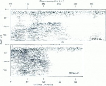
Fig. 11. Migrated 50 MHz surveys of study a along the 400 MHz line (profile a2) and perpendicular to it (a3). Arrows indicate where these lines cross and LM is the lake margin. Two englacial zones (1, 2) are seen above the basal zone (3) at the start of a3. The refections below about 70 m depth are of unknown origin.
In profile a2 of Figure 11, basal-ice reflections extend across the record between about 10 and 35 m depth. Profile a3, which parallels the direction of ice flow and starts further up-ice. shows the basal zone beginning at a depth of about 30 m and rising towards the surface as surface elevation decreases. Two englacial zones occur at the start of this profile; this type of feature will be seen and discussed in study c. Deep reflections in profile a2 at a depth of about 70 m are of unknown origin, and have too much interference to determine phase. A few scans at distances around 240 m and at a depth of about 75 m in profile a2 indicate a low-over-high contrast in dielectric constant. Therefore, these reflections are most likely associated with either an ice rock interface or a water horizon located a1 the bottom of over-ridden and glacier ice that has been buried within the basin. The absence of deep reflections beyond 300 m distance along a2. and along a3 as ii passes over the lake margin (LM on the profile: on to the ice-covered lake, is probably due to attenuation in wet, line-grain materials.
Study b: 100 MHz WARR Over Basal Ice
A wide-angle reflection and refraction (WARR) sounding was performed in 1991 in order to obtain a dielectric constant value (n 2) for basal ice by measuring the ground-wave velocity. The sounding was performed over an exposed, 50 m long section of debrisrich basal ice using the 100 MHz antennas. Reference Annan and DavisAnnan and Davis (1976) and Reference Arcone and DelaneyArcone and Delaney 1984 (have discussed this technique with several examples. Theoretically, several coupling modes are excited, including an air-wave traveling at speed c, a ground-wave retraction travelling at speed c/n, and several sub-surface reflections that may propagate modally if a sub-surface interface is within a depth of a few wavelengths. The dielectric constant is derived from the ground-wave speed.
WARR profile b1 in Figure 12 was obtained by recording while the receiver antenna was separated at an increasing distance from the fixed transmitter. The antennas were polarized normal to the profile direction. A second WARR reversed direction and gave identical results. The important events are the air and ground waves. Many sub-surface reflections, all of which appear eventually to parallel the ground wave, are also present. The ground-wave slope in Figure 12 can be seen to vary along the profile, but the average is 15.3 cm ns−1. This velocity corresponds to a dielectric constant of 3.8 (n = 1.95), typical of values found in massive silty ice in permafrost Reference Delaney and ArconeDelaney and Arcone, 1984; Reference Arcone and DelaneyArcone and Delaney, 1984, Reference Arcone and Delaney1989). The fact than the average n deviates only about 10% from the ice value 1.78. and than it is apparently variable over this small distance, others further justification for the application of single-layer migration to discontinuous structures beneath the englacial basal ice transition.

Fig. 12. Wide-angle refection and refraction profile b1 at 100 MHz over an exposed section of basal ice.
Assuming that most dry silicate particles have a dielectric constant that ranges between 4.4 the value for quartz) and 5.7 (feldspars), and using the cube-root dielectric-mixing formula of Reference Landau and LifshitzLandau and Lifshitz (1960), the value of 3.8 corresponds to a din content of 30–56% by volume. These content values appear high and. although they are possible, they are not probable. Samples from another, nearby exposure of basal ice contained an average of 20–30% debris by volume, but samples of individual layers and lenses of debris-rich ice (0.5–6.0 cm thick) ranged from about 10 to 75% debris by volume. It is more likely that the elevated dielectric constant is due to water adsorbed on silt particles or in small pockets.
Study c: Englacial and Basal Regimes; 50 MHz
This study was conducted on 9 April 1989 along a 220 m line parallel to the glacier flow. Snow conditions were highly variable, but at several locations and especially at 40–80 and 110–140 m, there was a layer of about 0.5 m of saturated snow. The profiles covered englacial-ice depths that deepened from a few meters at the ice margin to more than 60 m up-glacier. The basal ice was exposed at the margin (Fig. 13). We confined our work to 50 MHz pulses because at ice depths below about 20 m, 400 MHz surveys become too noisy due to the limited sampling rate available. The separable 100 MHz antennas were not available in 1989.

Fig. 13. Exposed section of englacial (light) over basal (dark) ice near study c.
The unmigrated and elevation-corrected profile c1 is shown in Figure 14. The profile is dominated by diffractions, as are other profiles taken perpendicular to the flow. Immediately beneath the DC in Figure 14 is a clear, englacial zone (1) of about 10–20 m depth. No strong reflections originate in zone 1 except for the mar-surface disturbance around 130 m from saturated snow and ice covering a moulin: difficulty towing the antennas may have distorted the record slightly in this segment. A second englacial zone (2) progressively thickens up-glacier and contains numerous small reflections and diffractions. The hyperbolically shaped diffraction peaks are broadened, as would be the response of an extended target. Zone 3 is a region of more intense reflections, with associated diffractions that define its apparent upper boundary. The intersection of this boundary with the ground surface further west, at the terminus (off left side of profile c1), coincided with the physical contact of the englacial-and basal-ice zones. The diffuse transition associated with the occurrence of multiple diffraction hyperbolas, the deepest peaks of which occur at about 800–1000 ns, may define an apparent location of the sole of the glacier, but there is no clear signal. The upper three-zone structure was seen in profile a3 and occurred repeatedly on profiles throughout the terminus region.

Fig. 14. Unmigrated 50 MHz profile c1 of the main line in study c. Several zones of different radar character (described in text) are numbered. Light bands are positive-phase and black bands are negative.
An extension of profile c1 was made to the west in order to identify reflections from the clear ice (lower ε) basal ice (higher ε) contact that was approaching the surface, A segment of this extension, profile c2, is shown in Figure 15 along with one of the scans. This particular scan was recorded with antennas on a smooth, hard ice surface. The basal-ice event consists of three strong half-cycles phased in a − + − sequence and establishes a wavelet form and phase reference for other events in profile c1; neighboring scans show this event to be followed by one weak half-cycle. For the particular relative antenna orientation, the first three DC: half-cycles are phased oppositely in a + − + sequence. Verification that this opposition in phase sequences indicates basal ice and not a void is provided in the Appendix by an example with phases that agree. The generation of this DC and the effect of high-pass filtering are also discussed in the Appendix.

Fig. 15. L ’nmigrated profile c2 (lop) which extended near the intersection of the basal ice with the surface, and scan 264 which identifies the transmitted waveform and phase from the basal-ice refection.
Asympototes of the early diffractions at the start of profile cl show the intensification of signal strength predicted by the H-plane directivity (Fig. 2) and confirm that most events originate close to the profile transect plane. T his off-axis strengthening of the signal will affect migration of these shallow diffractions as it did in study a. Scans containing events from the prominent diffraction that peaks at a distance of 45 m are shown in Figure 16. Scan 119 is at the peak of the hyperbola, and 104 and 88 are from oil-axis (44 ° for scan 88, assuming the diffractor was directly along the transect of the antennas). The off-axis pulse in scan 88 is much stronger in amplitude than is the pulse from the peak. The agreement in phase of the hyperbolic response with the DC indicates a high-over-low dielectric interface, presumably ice over an empty pocket or conduit.

Fig. 16. Selected scan segments containing the diffraction response (darkened) that peaks at about 45m distance in the unmigrated data of profile c1.
The migration of profile c1 is shown in Figure 17a. The migration used the velocity in ice and an aperture width of 38 m (101 scans), near the maximum width allowed by the software, which covers about 70% of the widest diffractions. The width encompasses the H-plane directivity maxima to a depth of only 28 m so that most of the record is migrated using only a small and therefore more uniform part of the directivity. The ice velocity generates hyperbolas that correctly match the slopes of the basal-ice diffraction asymptotes and thereby produces the longest segments of coherent reflections to define best the englacial basal ice transition. An extensive horizontal structure, possibly the glacier bed, occurs at a depth of about 90 m between distances of about 130 and 220 m and possibly extending further up-glacier. Generally, however, the migration produces many distinct horizons in zones 2 and 3. the lengths of which possibly affected the relatively small migration aperture at depth. The horizontal banding in the bottom 200 ns of the record appears to be remnants of internal low-frequency noise that were not completely filtered, such as in the lower left corner, where the spacing is very regular.

Fig. 17. (a) One-layer migration of profile c1 and (b) a 2D Fourier-transform filtered version that retains events that are only horizontal or slope down to the east. In the top figure, the early diffractions that originated within the first 150 scans of profile c1 are improperly migrated.
Many of the diffractions defining the top of zone 2 in profile c1 between 40 and 100 m appear to be partially or totally over-migrated in Figure 17a. This is partly due to the fact that asymptotes on only one side of most shallow-diffractions can be matched using ε = 3.2. Although a higher value of ε will improve the appearance of the migration of the two most prominent and shallow hyperbolas, the upper ten or so meters of zone 1 ice should be well frozen in early spring and not contain any intergranular water needed to elevate ε. Simple calculations show that it is also not possible for a thin (less than 1 m) layer of slush or even water to distort significantly a diffraction from 10m depth in ice. Part of the difficulty may lie in an irregular target geometry and Reference Lee, Jackson and MasonLee and others (1993) have proposed a scheme to compensate for this. Regardless of the ε value used, bow ever, apparent over-migration to about 20 m depth always occurs and is due to the antenna directivity seen in Figure 3.
A two-dimensional (frequency and wavenumber) Fourier-transform filtering of the migrated profile c1 is shown in Figure 17b. The filtering retains events that are horizontal or slope downward to the cast and, therefore, clarifies some of the more continuous interfaces and helps to isolate reflection events within individual scans (Fig. 18). More visible now in Figure 17b is the sloping reflector that begins at the surface at 0 m and dips to the east. The horizons that begin at the top of the basal zone-occur over an apparent thickness of about 40 m on both the west and east sides. This thickness could be inflated by at least 10% due to the higher dielectric constant of basal ice. if it is all basal ice. Previous measurements Reference LawsonLawson, 1979a, Reference Lawsonb) at the edge of the active ice have indicated a basal-zone thickness ranging from about 5 to more than 15 m. therefore, these horizons may represent basal ice thickened by ice-marginal overthrusting.

Fig. 18. Segments of scans from the profiles in Figure 17 illustrating waveform phase.
Events for which interfacial dielectric constants can be identified from the transmitted wavelet and its phase are seen in scans presented in Figure 18. The scans are extracted from the migrated profiles of Figure 17. Within these and many other scans, the choice of wavelet half-cycles to compare with the reference of Figure 15 is nearly as clear as it was for the higher-resolution 400 MHz profile a1. Almost invariably, each of the 1½ cycle, highlighted events is followed by a weaker, fourth half-cycle. The wavelets highlighted here and seen within other scans show many + − + phase sequences for zones 2 and 3. indicating voids. The − + − sequence indicating dirt-rich ice or water occurs primarily in basal zone 3. As with study a, the appearance of these wavelets, and the fact that their coherence can be followed in some cases fin-tens of scans, implies the existence of only one smooth surface associated with a particular target.
Some of the events in Figure 18 contain one or two cycles beyond the reference waveform from profile c2. Given a probable 1−2 m target thickness in this area, the greater length of the 50 MHz pulse allow s target-bottom reflections to overlap surface reflections. Some apparent resonances are seen in scans 497 and 562, and are associated with the extended linear reflectors between 130 and 220 m in the migration, the closely spaced reflections with the same phase polarity sequence of + − + that occurs in scans 213 and 497 are unusual because a progression of layers in which ε decreases with depth does not seem likely.
Figure 19 shows an interpretation of the events in the migrated profiles of Figure 17 for which phase could he determined. Open loops represent empty conduits, with no particular significance attached to the exact thickness of the loops. Grounded bars represent water or debris. The length of the loops and bar segments is at least 5 m, but this is only the length of the brighter events and may also reflect the small migration aperture at depth. The transition from basal ice to a fourth zone of sediments and/or bedrock is speculative. The fact that the upper “contact” between the zones of clear and englacial ice with scattered debris approximately parallels the ice surface suggests that the contact defines the active thermal regime, below which liquid water begins to occur within the ice. The upper, clear layer should have been frozen and/or dry in late winter, gradually becoming wetter toward the surface in spring. Conduits within the englacial zone ought to be clear of any water at the time of these investigations, as the radar data imply. This structure will be examined in more detail in a later publication I paper in preparation by D. F.. Lawson, S.A. Arcone and A.J. Delaney).

Fig. 19. Generalized interpretation of some of the events in the migrated profile c1. Clear enclosures represent probable conduits, and the grounded segments represent debris and/or water. The interpreted thickness of the basal zone may be generated by over thrusting along the ice margin. The depth seal, is based on propagation in ice and is probably too large for a single basal-ice zone.
Conclusions
The diffraction summation invoked in migration has been shown capable of both maintaining and recovering the form of the transmitted wavelet sufficiently to allow determination of whether or not it had changed phase upon reflection. Stacking and the short duration of the GPR wavelet affect recovery also, but the former depends on the amount of data recorded and the method of acquisition, while the lattter would become important in a reflection-rather than a diffraction-dominated profile caused by the presence of dielectrically “thin” layers. Future work will improve wavelet recovery by using a greater sampling density and 16-bit quantization to reduce errors that may have occurred due to the relatively primitive eight-bit analog to digital conversion.
A wider migration aperture should also improve wavelet recovery as well as the spatial imaging, but at the price of generating the migration noise discussed previously. Λ more uniform antenna directivity or a change in signal processing to correct for the directivity would improve imaging and wavelet recovery, and decrease migration noise; others are aware of the noise problem and have devised compensatory schemes to eliminate bright spots (personal communication from R. Jacobel). Changing directivity by profiling in the E-plane would risk phase aberrations at high angles of incidence (Reference ArconeArcone, in press). The complicated directivity of a single GPR antenna makes it doubtful that a fixed array could be designed to give a more uniform distribution of energy; larger, real antenna apertures are also subject to significant waveform degradation. Synthetic apertures Reference Fisher, McMechan and AnnanFisher and others. 1992a) greatly improve imaging, but are nut always practical. In view of the need lot a wide migration aperture to migrate deep reflections correctly and improve wavelet estimation, we think that Kirchhoff migration of GPR glacier profiles at least should use an obliquity lactor that also compensates for antenna directivity.
The recovered wave forms give evidence for a substantial number of voids within the englacial- and basal-ice zones at the time of these early-spring investigations. The frequent, isolated appearance in the migrated data of the transmitted-wavelet form and the continuity of events over depths to about 90m suggest many of these targets are characterized by a single smooth interface. The less frequent occurrence of closely spaced wavelets with opposite phases suggests that embedded, electrically thick layers are present. Recovery of wavelets to depths of 90 m implies little dispersion during propagation, but this may not hold true in late-summer surveys when the upper part of the glacier warms and drainage is fully developed. Resolution of basal-substrate reflections will require at least 50 MHz pulses, but the necessary time ranges will need a greater sampling rate than the 1024 samples per scan used here.
Acknowledgements
Support for this research was provided by the U.S. Army-Cold Regions Research and Engineering Laboratory Project 4A161102AT24, work unit AT24-SS-E10, two Inter-Laboratory Independent Research projects and the Cold Regions Water Resources Program, work unit CWIS32689. The authors gratefully acknowledge Dr Β. Narod of Vancouver, BC, and Professor R. Jacobel of St. Olaf College, Northfield, for their comprehensive and valuable reviews, and the field assistance of J. Strasser. Citation of brand names does not constitute official endorsement or approval of the use of such commercial products.
Appendix
Direct Coupling as a Phase Reference
The DC between transmitter and receiver antenna has been shown to be a suitable phase reference to substitute for a transmitted waveform. This section presents evidence that it is the air-wave component of the DC and the filtering applied to it that is the critical factor.
Theory (e.g. Reference AnnanAnnan. 1973 predicts that only near-field modes propagate along the surface from an antenna on the sin face of a dielectric half-space, although there is debate over which surface modes propagate in the near field of an antenna just above the ground surface (e.g. Reference Narod and ClarkeNarod and Clarke, 1994). The dominant modes are air and ground waves with opposite phase polarity and for which the field strength attenuates in inverse proportion to distance squared. Practically, the close proximity of transmitter and receiver antennas, the changes in ground dielectric structure in the very near field and the high-pass temporal filtering needed to eliminate gain variations due to inconsistent antenna ground contact can change the nature of the DC. We have observed, however, that the phase polarity of the first major half-cycle is consistently the same for a given antenna setup and filtering procedure, and that the DC waveform itself is similar to the waveforms of sub-surface reflections.
Pulse-EKKO 50 MHz
The above theory is consistent with observations of coupling between our own. specially constructed 50 MHz antennas situated at a water surface e.g. Sellman and others, 1993) and separated a few meters. An exemplary scan is shown in Figure 20, where it can be seen that the near-field air and ground modes have opposite phase polarity. The scan also contains a far-field sub-surface reflection from an interface between high-over-low dielectric permittivity media. The first few half-cycles of this reflection have the same phase polarity sequence as does the air wave. The reverse dielectric situation will produce a π phase shift, as was seen in Figure 15.

Fig. 20. Separation of surface-air and ground waves propagating between 50 MHz antennas separated 3.6 m on the surface of a lake. The air and ground waves have opposite phases. The bottom reflection is from sediments with dielectric constant lower than that of the water. Starting from the leading edge, the successive half-cycles of the air and bottom events have the same sequence of phase polarity. The trace is unfiltered and selective gain has been added to the surface modes to compensate for the nonuniform time-range gain.
The phase polarity of the DC and of any reflection also depends on the polarity of transmitter and receiver connections to the antennas, but this will not affect their relative phase. In study c the transmitter and receiver antennas were separated 2 m. On ice this separation corresponds to a delay between air and ground waves of about 5ns. which is sufficient time for the first half-cycle of the air wave to begin the DC. In the water study of Figure 20, the first half-cycle surge in the DC is negative, whereas in our studies on the ice Figure 21 from profile c2), the initial half-cycle surge in the DC is positive.
The leading DC half-cycle in Figure 21 is followed by-two more strong half-cycles and then one weaker one because the 2 m antenna separation on ice did not allow the air and ground coupling to overlap exactly. Our choices of sample width for high-pass filtering never produced an appreciably negative half-cycle at the leading edge Fig. 21). Consequently, in contrast with the filtered. 400 MHz data shown next, reflections from interfaces between media of low-over-high dielectric constant produced reflections π out of phase with the DC:.

Fig. 21. Waveforms before and after high-pass filtering, for the unshielded PulseEKKO 50 MHz antenna pair sitting on solid ice. The highlighted reflection is from basal ice and its phase is opposite that of the DC. The filtering also eliminates an offset to the overall gain.
400 MHz
The GSSI Model 3102 antennas are hardwired in place and back-shielded by connected, metallic, double half-cylinders capped at both ends. Through some clever engineering, the DC avoids resonance within the shielding. The shielding precludes any simple explanation for the generation of the DC: waveform, but the waveform shape and the closeness (about 15cm between feed points) of the antennas suggest it is controlled by the air wave. Any distinct air and ground coupling must virtually overlap. The first half-cycle of the unfiltered DC: is always negative Fig. 22 and is followed by a strong and then a weak half-cycle. Our choice of sample width for high-pass filtering always added a significant positive half-cycle to the leading edge of the DC pulse, but one of negligible amplitude to the sub-surface reflections. Consequently, in contrast to the unfiltered data and the 50 MHz results, the phase polarity sequence of the strongest DC half-cycles in filtered, Model 3102 data always appears the same as that of a reflection from the interface between low-over-high dielectric permittivity media.

Fig. 22. Waveforms before and after high-pass filtering, for the shielded Model 3102 400 MHz antenna pair sitting on solid ice. The highlighted reflection is from water, and its phase is the same as that of the DC.


