


1. Introduction
Turbulent boundary layers (TBLs) are ubiquitous in nature and technology, with significant implications concerning, among others, drag, heat and mass transfer, and aerodynamic noise generation. The majority of practical TBL applications, such as flows over wings, surface protrusions, dunes, mountains and vegetation, involve roughness. Additionally, these and many other industrial applications such as diffusers, nozzles, ducts, blowers, compressors and others also involve pressure gradients, which can have significant effects on the flow physics. Roughness and pressure gradient effects on canonical TBLs, not surprisingly, result in notable alterations to the near-wall TBL flow physics. Flow over a bump involves an adverse pressure gradient (APG) downstream of the bump and a favourable pressure gradient (FPG) upstream of the bump.
In the case of APG, the typical flat plate TBL is sufficiently altered such that the standard scaling laws in the outer region – the ‘log law’ and ‘defect law’ – do not hold (Tanarro, Vinuesa & Schlatter Reference Tanarro, Vinuesa and Schlatter2020). Furthermore, for increasing APGs, the streamwise Reynolds stress in the outer region increases and progressively develops a second outer peak outside the usual buffer layer peak (Skåre & Krogstad Reference Skåre and Krogstad1994; Monty, Harun & Marusic Reference Monty, Harun and Marusic2011; Lee Reference Lee2017).
Flow separation caused by strong APG in internal or external flows continues to have numerous unanswered questions and remains an active research area; see, for example, Simpson (Reference Simpson1996), Krogstad & Skåre (Reference Krogstad and Skåre1995) and Cheng, Pullin & Samtaney (Reference Cheng, Pullin and Samtaney2015). Na & Moin (Reference Na and Moin1998a) numerically demonstrated that the well-known detachment and reattachment points of the separation bubble (SB) oscillate both temporally and spatially due to Kelvin–Helmholtz instability of the shear layer above the SB. Mohammed-Taifour & Weiss (Reference Mohammed-Taifour and Weiss2016) experimentally showed that the spanwise vortices are responsible for inducing a high-frequency unsteadiness of the detachment and reattachment points of the SB.
In our study, in addition to the separated flow downstream of the bump, the upstream flow necessarily involves an FPG, which has two interesting aspects: flow acceleration induced possible re-laminarization (Balin & Jansen Reference Balin and Jansen2020) and flow curvature induced (incipient) separation (Simpson Reference Simpson1996).
Wall roughness is central to TBL flow physics because of its role in skin friction and form drag (Leonardi et al. Reference Leonardi, Orlandi, Smalley, Djenidi and Antonia2003), and it will definitely alter the effects of pressure gradients. Numerous studies have concentrated on streamwise-aligned riblets due to their potential for reducing skin-friction drag in TBLs (Choi, Moin & Kim Reference Choi, Moin and Kim1993; García-Mayoral & Jiménez Reference García-Mayoral and Jiménez2011). Lin, Howard & Selby (Reference Lin, Howard and Selby1990) experimentally showed that in the case of a separation bubble behind a ramp (smooth, sigmoid-like backward step), the addition of longitudinal V-shaped grooves (riblets) placed at the beginning of the ramp shortens the bubble length. Similarly, transverse or longitudinal grooves placed rearward of bluff bodies can reduce form drag (Howard & Goodman Reference Howard and Goodman1985, Reference Howard and Goodman1987). Recent experiments by Simmons et al. (Reference Simmons, Thomas, Corke and Hussain2022) have examined the TBL with APG and large-scale flow separation over a smooth two-dimensional convex (backward-facing) ramp with sidewalls detailing the highly three-dimensional flow through inspection of near-wall topography and topology of both separation and reattachment. Their study highlights that two counter-rotating vortical structures (secondary flow) dominate the resulting flow separation. The secondary flow described by Simmons et al. (Reference Simmons, Thomas, Corke and Hussain2022) may relate to that occurring at a smaller scale on top of the longitudinal grooves; this secondary flow will be examined here in some detail. Song & Eaton (Reference Song and Eaton2002) (experimentally) and Wu & Piomelli (Reference Wu and Piomelli2018) (numerically) found that a TBL with a strong APG over a random rough surface results in earlier flow separation and delayed reattachment, contrasting that of an organized roughness such as riblets.
We investigate the physics of (separated) TBL over a bump with small-scale, organized roughness over the entire wall. More specifically, the physics of the near-wall turbulence, with pressure gradients, flow separation (and reattachment) over a transversal, sinusoidal bump with small-scale longitudinal square grooves is examined and compared with a smooth bump case. The flow over longitudinal grooves with pressure gradients and flow separation has not yet been addressed – hence the thrust of this paper.
2. Flow configuration and numerical method
The flow geometry is shown in figure 1: a precursor simulation (figure 1a), which connects smoothly (i.e. without any jump) with the main simulation domain (geometry detailed in figure 1b), is employed to provide the inflow. Unless stated otherwise, all quantities are non-dimensionalized using the bulk velocity ( $U_b$, flow rate/channel cross-section area), channel half-height ( $H$), density ( $\rho$, set equal to one) and the kinematic viscosity ( $\nu \equiv \mu /\rho$, where $\mu$ is the dynamic viscosity); dimensional variables are starred. In SW, the computational domain sizes ( $L_x, L_y, L_z)$ of the precursor and main simulation are respectively ( $6, 2, 1.6$) and ( $12, 2, 1.6$) in the streamwise ( $x$), wall-normal ( $y$) and spanwise ( $z$) directions. Note that at any $x$, the vertical height from the wall is denoted as $Y$;
$Y$;  $Y$ is equivalent to $y$ away from the bump but not over the bump. Additionally, $y$ is the distance from the flat bottom wall, independent of the bump, as shown in figure 24.

Figure 1. Computational domain and boundary conditions. (a) Precursor channel flow simulation domain with periodic boundary conditions in the streamwise ( $x$) and spanwise ( $z$) directions; (b) main channel flow simulation domain; (c,d) bump details with panel (c) emphasizing that $Y$ is vertical coordinate and not normal to the local bump surface and panel (d) delineating the height and length of the bump; (e) bump isometric view; (f) cross-sectional geometry of the grooves showing crest, crest corner and groove.
Bump profile. The TBL is perturbed by a transversal, sinusoidal bump, placed on the bottom wall (figure 1b). The sinusoidal geometry of the bump is defined by
 \begin{equation} f(x)= \begin{cases} \dfrac{h}{2} \sin\left[\dfrac{2{\rm \pi}}{\lambda_b}(x-x_s)-\dfrac{\rm \pi}{2}\right]+\dfrac{h}{2}, & x_s\leqslant x \leqslant x_s+\lambda_b, \\[10pt] 0, & {\rm otherwise}, \end{cases}\end{equation}
where  $x_s$ is the starting location of the bump, $h$ the maximum height of the bump and $\lambda _b$ the total length of the bump, i.e. one sinusoidal wavelength (figure 1c). The parameter $x_s$ is chosen to be $3.5$ – far enough from the inlet so that the flow modified by the bump does not discernibly modify flow at the inlet. The height of the sinusoidal bump is $h=0.15 (h^+=45)$ and the length is $\lambda _b=1.5 (\lambda _b^+=450)$. Hereinafter, the superscript $+$ denotes non-dimensionalization by the friction velocity $u_\tau ^*\equiv \sqrt {\tau _w^*/\rho }$ at the inlet and the viscous length scale $\nu /u_\tau ^*$, where $\tau _w^*$ is the wall shear stress (see Appendix B for details on the computation of $\tau _w$). The bump height is relatively large but no more than the buffer layer height (note that the bump length is even larger – $10$ times the bump height $h$ and $30$ times the groove width $w$), and the bump induces a notable flow separation bubble, but it is sufficiently small such that the top wall TBL is minimally affected (without inducing any separation on the top wall, as well as keeping the alteration of the wall shear stress at the top wall to ${<}0.4\,\%$ of a flat wall smooth channel, further discussed in § 4.3).
Longitudinal square grooves are incorporated throughout the bottom wall of the whole domain both in the precursor and the main domains, while the top wall remains flat and smooth. Note that (2.1) corresponds only to the profile of the crest, and since the groove cross-section is exactly the same throughout the entire computation domain  $L_x$, the groove's bottom portion is not a sine curve. The grooves consist of identical repeats of square cavities along the $z$ direction, each with equal crests and troughs of width $w=0.05$; the groove depth is $k=0.05$ (figure 1f). Between SW and GW, the computational domain is the same, except in GW, where the bottom wall extends downward by the groove depth; i.e. $L_y$ in GW is larger by the groove depth. The square groove size in wall units is $k^+=15$, found to reduce skin friction drag (without bump) by $3.3\,\%$, with the grooves behaving as a riblet-like surface. A set of simulations with a smooth wall boundary condition (i.e. with the bump but no grooves) was also performed to compare all (instantaneous and statistics) flow measures and analyse the effects of the grooves.
We perform direct numerical simulation (DNS) of the non-dimensional incompressible Navier–Stokes equations,
 \begin{equation} \frac{\partial U_i}{\partial t}+\frac{\partial U_i U_j}{\partial x_j} ={-}\frac{\partial P}{\partial x_i}+ \frac{1}{Re_b}\frac{\partial^2U_i}{\partial x_j^2} +f_i; \quad \frac{\partial U_j}{\partial x_j}=0, \end{equation}
where  $U_i$ is the velocity component in the $i$th direction, $f_i$ is a forcing vector term to model a solid body (i.e. the bump and crests) using the immersed boundary method (Fadlun et al. Reference Fadlun, Verzicco, Orlandi and Mohd-Yusof2000), $P(=P^*/\rho U_b^2)$ is the non-dimensional pressure with $P^*$ denoting pressure and $Re_b(\equiv U_b H/\nu )$ is the bulk Reynolds number.
The equations are solved using a second-order finite difference scheme for spatial derivatives and a third-order Runge–Kutta algorithm for the time stepping combined with the fractional-step method. The numerical method details can be found from Orlandi (Reference Orlandi2000) and Orlandi & Leonardi (Reference Orlandi and Leonardi2006). Periodic boundary conditions are applied in the spanwise ( $z$) direction. The inflow boundary condition is obtained from the precursor simulation of the channel flow with periodic conditions in $x$ and $z$ (figure 1a) at the bulk Reynolds number $Re_b=5300$ (friction Reynolds number $Re_\tau \equiv u_\tau ^* H/\nu =300$). Between SW and GW cases, the bulk Reynolds number is kept the same at the inlet of the channel. Note that grooves add 1.25 % to the total channel cross-sectional area; that is, the maxima of the mean velocity profiles between GW and SW are slightly different – but not of any significance. The outflow boundary condition is ${\partial U_i}/{\partial t}+C {\partial U_i}/{\partial x}=0$, where $C$ is chosen to be the maximum instantaneous streamwise velocity at the channel exit plane in the previous time step of each computation step (Orlanski Reference Orlanski1976). The no-slip condition is imposed on both the top and bottom walls. Details of the computational grid are in Appendix A and computational validation is in Appendix B.
3. Instantaneous flow field example
Figure 3(a) depicts a snapshot of the instantaneous streamwise velocity in an  $x$–
$x$– $y$ plane of the entire computational domain for SW, showing the bump's relative size and perturbation of the flow. A shear layer starts near the bump peak (figure 2, R3), overlying the SB, and subsequently rolls up into spanwise rollers; the rollers undergo pairing and tearing, and interact with the SB structures before the reattachment. In figure 3(b), we see only three large-scale swirling regions within the SB – these swirling regions change with time, varying between 3 and 5 structures. Also, vortex dipoles are present around and inside the SB. They are not evident in the streamlines, but can be identified through the vorticity and corresponding pressure fluctuation field (figure 3c,d). The dipoles are expected, given the proximity of the shear layer to the wall, as the spanwise rollers would detach vorticity from the wall. The dynamics of these inherently unsteady vortical structures within the bubble, coupled with the grooves-induced secondary flows, presents a highly complex flow of interacting vortical structures and is the focus of our study.

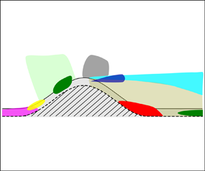
Figure 2. Schematic denoting the regions of interest and important flow features as a summary. I – upstream separation; II – incipient separation; IIIab – negative production; IV – favourable pressure gradient (FPG); V – adverse pressure gradient (APG); VI – spinning jets; VII – shear layer; VIII – separation bubble; IX – minibubble.

Figure 3. A sample instantaneous flow field. (a) Colour map of streamwise velocity in an  $x$–
$x$– $y$ plane for the full domain SW bump case at $z=L_z/2$. Zoomed-in views of instantaneous $x$–
$x$– $y$ plane contours of: (b) SW streamwise velocity; (c) SW spanwise vorticity; (d) SW pressure fluctuations; (e) GW streamwise velocity; (f) GW spanwise vorticity; and (g) GW pressure fluctuations. Isometric views of instantaneous streamlines over the GW show (i) flow channelling into the grooves and (h) flow ejection (blue originating below the crest and red above). The letter markers identify locations of specific flow features: (M) secondary recirculation bubble (minibubble), (R) shear layer rollup, (P) vortex pairing, (D) vortex dipole and (T) vortex tearing.
A groove alters the flow by channelling fluid into the groove on the upstream side of the bump (figure 2, R2) and also jetting fluid out of the groove immediately after the peak of the bump (figure 2, R3) – illustrated in figure 3(h,i) via instantaneous streamlines colour-coded by the  $Y$-distance from the crest (blue below the crest and red above). The initiation of the shear layer is pushed upwards in GW because of the jetting of the fluid from the grooves (compare figure 3c,f). Inside the SB of GW (figure 2, R4), we often find smaller vortical regions attached to the wall with opposite signed circulation to that of the shear layer rollers as well as the SB (figure 3e–g); we call them ‘minibubbles’, further discussed later. Although a minibubble is not present for the SW snapshot in figure 3(b–d), they do occur intermittently for SW. Despite the low speed in the separated region, the flow channelling within the grooves and the minibubble (figure 3e,i) significantly modify the drag (discussed later). Note that the instantaneous reattachment length in GW is larger than in SW. We will see later that this is also the case for the mean SB.
Figure 4(a–d) show the streamwise velocity fluctuations,  $u=U-\bar {U}$, on the curved surface parallel to the (SW and GW) bump at $Y=0.01 (Y^+\approx 3)$ and $Y=0.033(Y^+\approx 10)$. The overbar $\overline {({\cdot })}$ denotes the average over time and the spanwise ( $z$) extent at every $x$ and $y$ location within the domain. The dashed lines A-A, B-B and C-C indicate the start, peak and end of the bump, respectively. In SW (figure 4a,c), the typical (low-speed) streaks are present near the channel inlet (figure 2, R1), and the characteristic length scales (in both streamwise length and spanwise spacing) agree with those found in documented flat wall turbulence (Kim, Moin & Moser Reference Kim, Moin and Moser1987). In SW, near the peak of the bump, the flow detaches around $x=4.4$ (indicated by the zero-shear stress wiggly black thick line in figure 4a,e). Note that all streaks disappear a short distance behind this separation line, and velocity fluctuations of the upstream flow become very weak past this point (more apparent in the zoomed-in view in figure 4e), to be expected in this decelerated flow (Simpson Reference Simpson1996).

Figure 4. Instantaneous colour maps of streamwise velocity fluctuation,  $u$, in an $x$–
$x$– $z$ plane: (a) SW at $Y^+=3$; (b) GW at $Y^+=3$; (c) SW at $Y^+=10$; and (d) GW at $Y^+=10$. Zoomed-in views of the dotted regions in panels (a,b): (e) corresponding to panel (a) for SW and (f) corresponding to panel (b) for GW. Zoomed-in views of $u$ in an $x$–
$x$– $z$ horizontal plane at $y^+=48$ for (g) SW and for (h) GW. Recall that $Y^+$ measures vertical distance from the bump surface, while $y^+$ denotes constant horizontal surface; hence panels (e,f) are parallel to the bump surface, while panels (g,h) are horizontal surfaces capturing the shear layer structures. The solid thick lines in panels (a–h) denote the SB detachment and reattachment. The thin line contours in panels (e–h) denote constant $u$ values: $0.02$, solid; $-0.02$, dotted. Line A-A identifies the start of the bump, B-B the bump peak and C-C the end of the bump.
Past the SW bump ( $x>5$), streamwise velocity fluctuations persist without streaks with a significant increase in magnitude due to the reattaching shear layer. While the detachment is uniform in the spanwise direction, the turbulent reattaching shear layer (with embedded spanwise vortices) induces some spanwise inhomogeneity of the instantaneous reattachment line (figure 4e) – overlooked in the averaged flow field.
In contrast, the streaks in GW far upstream (figure 2, R1) and downstream of the bump have weak spanwise modulations due to the grooves at  $Y^+\approx 3$ (figure 4a) (caused by the streamwise swirls at the crest corners; see Arenas et al. Reference Arenas, García, Fu, Orlandi, Hultmark and Leonardi2019); but this modulation disappears away from the wall ( $Y^+\approx 10$, figure 4b). The (random) streaks persist past $Y^+=10$ with spanwise spacing and streamwise length the same as in SW (see figure 4c,d). The grooves’ modulation may be more important for different groove sizes, either larger or smaller, but is not explored here.
A notable feature for GW (unlike in SW) is the small-scale streaks downstream of the bump's peak ( $x\simeq 4.2$, figure 4b,f) generated by the flow channelling. Clearly, the groove-induced streamwise velocity fluctuations, $u$, are strong at the bump's peak and diminish moving downstream in $x$ near the wall at $Y^+=3$ (figure 4f) and across the shear layer in $z$ at $y^+=48$ (figure 4h). In the reattachment region ( $5.5< x<6$), $u$ (at $Y^+=3$) for GW are similar to those for SW, i.e. the groove-induced $u$ completely disappear. Interestingly, the reattachment line – which reflects the presence of grooves – has no correspondence with $u$ at $Y^+=3$ (figure 4f) and hence there is no significant bottom-up effect, presumably because of the flow stagnation around the reattachment point.
A perspective in terms of  $\lambda _2$ vortical structures (Jeong & Hussain Reference Jeong and Hussain1995) is shown in figure 5 to better separate vortices from shear layer vorticity (in contrast to figure 3c,f). As the typical near-wall quasi-streamwise vortices (Robinson Reference Robinson1991) approach the (SW) bump, they follow the wall curvature and become stretched due to flow acceleration. Then, they drastically weaken after the bump peak when facing flow deceleration (compression) due to the APG (see figure 15a) – consistent with the vanishing streaks in figure 4(a). After the streaks vanish, spanwise vortices (rollers) develop in the shear layer from the peak of the (SW) bump, along with numerous spanwise arch vortices (not hairpins) and finer-scale structures in the SB (figure 5c,e). The increased velocity fluctuations noted earlier are detailed by the myriad of small-scale $\lambda _2$-structures emerging in the separated bubble. After reattachment (around $x=5.5\unicode{x2013}6$), where new streaks begin to re-emerge, the vortical structures are a mixture of fine-scale structures and newly generated quasi-streamwise vortices. Far downstream of the (SW) bump (figure 2, R5), the boundary layer gradually relaxes to a flat wall channel flow state, and quasi-streamwise vortices are the prevalent structures near the wall (figure 5a).

Figure 5. Instantaneous iso-surfaces of  $-\lambda _2=3$ vortical structures coloured by streamwise vorticity $\omega _x$ for (a) SW and (b) GW. (c–f) Zoomed-in views of $-\lambda _2=4$ iso-contours coloured by streamwise velocity $U$:(c,e) SW and (d,f) GW.
For GW, the vortices far upstream and downstream of the bump are very similar to SW, confirming that the GW does not significantly modify the streaks and overlying structures on a flat surface. However, near the peak of the bump, numerous small streamwise structures are observed to be attached to the grooves’ corners (figure 5d,f), which are associated with the flow channelling through the grooves. The corner structures predominantly connect to the rollers in the developing shear layer (figure 5f). While the rollers are the dominant contributors to turbulence intensity and production in the SW developing shear layer, the corner vortices connecting to these rollers play a significant role in GW. Here, we focus only on their significance to flow statistics, while in a subsequent paper (García et al. Reference García, Hussain, Yao and Stout2024), we will address the spanwise rollers and streamwise groove corner vortex dynamics in more detail.
4. Flow statistics
4.1. Mean flow field
To understand the underlying effect of the grooves, consider  $\langle U\rangle$, which denotes the value of $U$ averaged over all grooves at the same relative point and averaged over 500 flow realizations, which are sampled one non-dimensional time unit (i.e. $H/U_b$) apart. Figure 6(a–d) show the colour maps of the mean streamwise velocity (in $x$–
$x$– $y$ planes), both $\langle U \rangle$ and $\bar {U}$, superimposed with the corresponding mean streamlines around the bump ( $3\leqslant x \leqslant 6.5$) for (a) SW and (b–d) GW.

Figure 6. Contours in  $x$–
$x$– $y$ planes of mean velocity components (a,b) $\bar {U}$, (c,d) $\langle U\rangle$, (e,f) $\bar {V}$ and (g,h) $\langle V\rangle$ superimposed with corresponding mean streamlines, where the thick red line denotes the mean dividing streamline; dashed line contours for $\bar {U}$ and $\langle U\rangle$, and solid line contours for $\bar {V}$ and $\langle V \rangle$. (a,e) SW and (b–d), (f–h) GW; (c,g) GW $x$–
$x$– $y$ section at the crest centre and (d,h) GW $x$–
$x$– $y$ section at the trough centre. The vertical dotted line corresponds to the $x$ position of SW separation, slightly after the bump peak.
Let us focus on the 2-D mean flow only. We consider  $x$–
$x$– $y$ planes at the centre of the groove and centre of the crest; note that by symmetry, $W$ is zero in these two planes, resulting in a purely 2-D flow. In these two planes, the separation and reattachment points are identified by the locations of zero wall shear stress $\tau _w$. The separating streamline starting from the separation point and the reattachment streamline ending at the reattachment point must be identical where they meet in between; otherwise, the SB cannot be steady. Hence, this line is used as the outer boundary of the SB. Various other criteria for determining detachment and reattachment, such as intermittency of backward flow, near-wall velocity vector angle and the effect of roughness, are discussed in the supplementary material (S1) available at https://doi.org/10.1017/jfm.2024.465. Although there are several co-rotating swirling motions and, in some instances, a minibubble attached to the wall in the instantaneous flow field (figure 3e), mean flow for SW (figure 6a) only displays a single SB.
The mean detachment location in  $\bar {U}$ (figure 6b) is slightly altered by the grooves (which has implications on the bump's form drag, discussed in § 4.3). The locations of detachment and reattachment vary along the spanwise direction for GW (figure 6c,d at the crest and trough, respectively). In particular, detachment occurs slightly earlier in the troughs than on the crests, but the reattachment reverses this order – resulting in a longer recirculation bubble in the troughs compared with the crests. Furthermore, the spanwise variation of $\Delta x$ between the adjacent crest and trough detachment points is much smaller than that of the reattachment points. The spanwise variation of the detachment points is related to the counter-rotating streamwise swirling flow at each crest corner, discussed in § 4.2. The most significant effect of the grooves is to delay the bubble reattachment.
Upstream separation. A less prevalent but significant feature is the intermittent flow separation (not visible in the mean streamlines) at the upstream end of the smooth bump despite a favourable streamwise pressure gradient in the centre of the channel. A mean streamline curvature is associated with a pressure gradient across the streamline obeying the transverse Bernoulli equation  $\partial \langle P^*\rangle /\partial n^*=\rho \langle U_s^*\rangle ^2/R^*$ (at each point of the streamline, $R$ is the radius of curvature, $n$ the coordinate normal to the streamline and $U_s$ the speed along the streamline – strictly, in the inviscid sense). The curvature of the streamline causes an APG in the upstream side of the bump, i.e. $\partial \langle P\rangle /\partial x>0$ along the wall in the converging flow region, whereas the free stream flow is accelerating, i.e. $\partial \langle P\rangle /\partial x<0$ (see in figure 9a,d that $\partial \langle P\rangle /\partial s<0$ along the free stream streamline versus $\partial \langle P\rangle /\partial s>0$ along the streamline near the wall at $x=3.5$). To reaffirm, while the free stream flow is accelerating, there is an APG along the wall as the flow approaches the bump – hence, the possibility for counterintuitive flow separation.
The mean streamlines in figure 6(a–d) suggest there is upstream separation only for GW. However, even though no upstream mean flow separation occurs for this SW bump height, a mean separation is very likely to occur for a higher bump, i.e. large  $h$, as well as for a shorter bump with a steeper slope – an important consideration in the design of wind tunnel contractions and nozzles.
Intermittent separation upstream of the bump for SW is detailed (figure 8) in terms of the instantaneous wall shear stress  $\tau _w$ and the flow field (this separation is also apparent in the instantaneous $P(x)$, although $\partial P^* /\partial n^*$ computed at this instant does not match $\rho U^{*2}_s/R^*$, as the flow is highly unsteady). The time series of $\tau _w$ (figure 8a) shows that positive shear stress ( $\tau _w>0$, in red, also reflected by the red region in the probability density function (p.d.f.) in figure 8c) occurs more often than negative shear stress ( $\tau _w<0$, in blue, reflected by blue in the p.d.f.); the negative minima are smaller in magnitude than most of the more numerous red maxima – the red maxima are typically approximately 3.8 times the blue minima.
While apparently intriguing, the skin friction increase due to sweep events is much more than the decrease by ejection events induced by streamwise vortices, and hence reflect the inherent sweep ejection asymmetry effect on the skin friction (Jeong et al. Reference Jeong, Hussain, Schoppa and Kim1997; Schoppa & Hussain Reference Schoppa and Hussain2002). These features are well captured in the p.d.f. of  $\tau _w$ at a particular location ( $x=3.5,z=1.35$) in SW – showing that the peak of the p.d.f. occurs mostly to the left of $\overline {\tau _w}$ in figure 8(b). Also shown (dashed line in figure 8b) is the p.d.f. of $\tau _w$ of all ( $640$) points in $z$ at $x=3.5$ for all ( $500$) realizations. Because the p.d.f. is based on a very long flow time, the occurrence of sweep and ejections should be stationary. The p.d.f. of our localized sample and the p.d.f. of the entire $z$ range are quite congruent, implying that our data are not biased by the detection point being preferentially on one side of a streak. Somewhat surprisingly, the two p.d.f.s around the peak match exactly (figure 8b) – this congruence confirms the expectation that the statistics, particularly p.d.f., is independent of $z$. The tails for the selected $z$ location have unavoidable fluctuations, which are significantly reduced in the dashed curve because it covers a much larger ensemble ( $640$ times). The integral of the blue region (negative wall shear stress, i.e. $\tau _w<0$) amounts to 9.6 % of the total integral of the p.d.f. – the upstream separation ( $\tau _w<0$) is intermittent and infrequent (figure 8a), not unexpected for this small curvature upstream of the bump.
The asymmetric p.d.f. of  $\tau _w$ (with skewness of $+1.004$) seems to be a consequence of the near-wall streamwise vortices having sweeps inherently stronger than ejections, as previously mentioned, i.e. the longer right tail of the p.d.f. Coincidentally, the wall shear stress in flat wall channel flows (without APG) also has skewness of ${\sim }1$ (Nakagawa & Nezu Reference Nakagawa and Nezu1977; Kim et al. Reference Kim, Moin and Moser1987); surprising because one would expect the TBL with an APG would modify the level of asymmetry of the p.d.f. of $\tau _w$. The kurtosis of $\tau _w$ in figure 8(a) is $4.96$, also very close to that of flat channel flows (Alfredsson et al. Reference Alfredsson, Johansson, Haritonidis and Eckelmann1988). These two coincidences are unexpected and may suggest that the intermittent flow separation does not significantly alter the near-wall streamwise vortices – a topic that remains to be explained.
The top view of instantaneous  $\tau _w$ in figure 8(c) illustrates an extreme event with minimum $\tau _w$ (marked by the vertical dashed line in figure 8a), showing that the upstream separation is highly non-uniform in $z$, in addition to being intermittent, unlike the SB downstream which is uniform in $z$. The $x$–
$x$– $y$ section in figure 8(d) (corresponding to the solid grey line in figure 8c) reveals that the SB is extremely thin and does not significantly affect the overlying coherent structures. The small streamwise extent of this upstream recirculation region has a peak in the $\omega _z$ contours (dotted lines, figure 8d) in contrast to the streamwise extended vorticity layer above the SB downstream (figure 3c). Moreover, the streamlines in figure 8(d) have a spiral-like pattern (focus, at $x\simeq 3.43,y\simeq 0.005$), and hence with a strong spanwise velocity; no such spanwise motion is evident in the downstream SB. Here, we emphasize that flow separation due to streamline curvature is relevant to wind tunnels (upstream of the working section), flow over dunes, bumps, large-scale roughness, etc.
Intermittent flow reversal is a known behaviour within flat plate longitudinal grooves TBL flows (Chu & Karniadakis Reference Chu and Karniadakis1993). Here, we see that the APG (due to streamline curvature) in GW induces a steady upstream separation within the grooves, i.e. a mean SB around  $x=3.5$ (figure 6d). Notably, the near-wall mean streamline curvature is lower in GW than in SW, resulting in a lower wall pressure in GW, and hence slightly decreases the APG with respect to SW at $x=3.5$ (figures 9e and 15a). Interestingly, the APG at the grooves remains strong enough to cause the upstream mean SB at the centre of the grooves. We speculate that this phenomenon is the combined effect of the APG and the inherent flow reversal of grooves that, when superimposed, leads to a steady separation at the centre of grooves. Note that on the crests, although there is no mean separation (figure 6c), intermittent separation indeed occurs.
Secondary bubble. Surprisingly, on the downstream end of the bump, there is also a small and steady separation bubble (‘minibubble’) within the grooves. It is embedded within the SB (at  $x\simeq 4.8$), having a circulation opposite (counterclockwise) to that of the much larger SB. Also, it is surprising that in the instantaneous flow for GW (figure 3e), a swirl with counterclockwise rotation can be identified (at $x\simeq 4.8$), which is the opposite direction of rotation to all the other swirls within the instantaneous SB. The generation mechanism of this minibubble appears to be similar to that of the upstream SB. Adjacent to the wall, the larger SB behind the bump has an upstream-directed flow before the reattachment point; as this flow approaches the bump, it induces a reverse APG (due to streamline curvature), resulting in flow separation. Additionally, while it is intermittently present at the crests (and also as in SW), the minibubble is apparently steady and not moving within the grooves – indicating that the grooves stabilize the minibubble (see figure 3f). The immobility of the minibubble is presumably due to the fact that the flow of the SB near the wall pushes it upstream, while its own image vortex under the solid surface pushes it downstream.
The effect of grooves on the mean velocity field is further documented through the mean wall-normal velocity component (figure 6e–h). Directly after the bump's peak, a negative patch of  $\langle V\rangle$ is observed at crests (downwash) along with the delayed detachment (figure 6g), while positive $\langle V\rangle$ at grooves (upwash) is associated with an earlier detachment (figure 6c). These are features connected with the streamwise swirling motion (§ 4.2) induced by grooves. The peak value in $\langle V\rangle$ located above the SB and near reattachment is shifted downstream in GW, consistent with the delayed flow reattachment.
The mean velocity profiles at various streamwise positions, extracted from figure 6, are shown in figure 7. For the  $\langle U\rangle$ profiles, the effect of GW is most noticeable in the near-wall region – particularly near the bump – where $\langle U\rangle$ is higher at the troughs than crests. All profiles collapse far from the wall for both SW and GW – emphasizing that the localized effect of the grooves does not modify the overlying flow. From $x=5$ to $5.5$, an overall decrease in $\langle U\rangle$ is observed in the shear layer region (i.e. in the range of $Y=0.1\unicode{x2013}0.2$, $Y\approx 0.15$) in GW. This decrease of $\langle U\rangle$ results from a higher skin friction drag induced by the grooves (upstream) at the bump's peak (figure 13a) and hence the reduced momentum downstream (at $x>5$). GW alters the mean streamwise stretching rate ( $\partial \langle U\rangle /\partial x$) in the developing shear layer (the flow accelerates as it channels into the grooves and decelerates as it ejects out of the grooves), which in turn affects turbulence production from Reynolds normal stresses via stretching, to be discussed in § 5.2.

Figure 7. Mean velocity profiles: (a) streamwise,  $\bar {U}$ (SW) and $\langle U\rangle$ (GW); and (b) wall-normal, $\bar {V}$ (SW) and $\langle V\rangle$ (GW), at different $x$. Red lines denote the SW case and blue lines denote GW at the crest (dotted), at the trough (dash-dotted) and spanwise averaged (dashed).

Figure 8. Incipient separation details in SW. (a) Wall shear stress  $\tau _w$ as a function of time and(b) probability density function (p.d.f.) of $\tau _w$ at a location $(x,z)=3.5, 1.35$ for SW – circles denote p.d.f. at $z=1.35$ for all realizations, while the dashed line denotes additionally averaging in $z$. (c) Top view of instantaneous colour contours of wall shear stress $\tau _w$ at the time ( $\times$) marked in panel (a). (d) Instantaneous colour map of streamwise velocity superimposed with line contours of instantaneous $\omega _z$ (dotted lines denote $-\omega _z$, dashed lines $+\omega _z$) and the instantaneous streamlines in the $x$–
$x$– $y$ plane (solid lines) at $z=1.35$ marked with a solid grey line in panel (c).
The effect of grooves is further detailed in the  $\langle V\rangle$ profiles. At $x=3.575$, while $\langle U\rangle$ profiles show an increase near the wall for GW, $\langle V\rangle$ decreases at all $y$ (figure 7a,b), i.e. the upward deflection is suppressed as the flow is channelled. Also detailed is the variability of $\langle V\rangle$ in the $z$ direction near the wall at $x=4.5$, as noted earlier, with $\langle V\rangle$ negative at crests and positive at troughs. Around the reattachment point ( $x=5.5$), within grooves, $\langle V\rangle$ increases abruptly in magnitude, consistent with a flow channelled upstream at high speed (figure 7a) at $x=5.25$.
Mean pressure. For  $P$ in figure 9, we chose a reference pressure $P_0$ such that $\overline {P-P_0}$ in the outflow plane is zero at the wall for SW and zero at the crest for GW; henceforward, $\langle P\rangle$ stands for $\langle P-P_0\rangle$ and $\bar {P}$ for $\overline {P-P_0}$.

Figure 9. Colour map of mean pressure in the  $x$–
$x$– $y$ plane for: (a) $\bar {P}$ for SW and (b) $\langle P\rangle$ for GW at the centre of grooves. (c) Colour map of $\langle P\rangle$ in the $x$–
$x$– $z$ plane (top view) at $Y^+=3$ for GW, over $1$ groove and crest. Measures computed along the selected streamlines (at three arbitrary distances from the wall – two near the wall and one farther away) shown in panel (a) for SW and panel (b) for GW: (d) $\bar {P}$ for SW, $\langle P\rangle$ for GW; (e) $\partial \bar {P}/\partial s$ for SW, $\partial \langle P\rangle /\partial s$ for GW; (f) velocity along the streamlines $U_s$; (g) curvature $1/R$ ( $R$ is the radius of curvature of the streamline); (h) $\partial \bar {P}/\partial n$ for SW, $\partial \langle P\rangle /\partial n$ for GW. Measures and streamlines in panels (a,b) have the same colour and line style.
We now discuss the mean pressure field,  $\langle P\rangle$, streamwise pressure gradient, $\partial \langle P\rangle /\partial s$, and normal pressure gradient, $\partial \langle P\rangle /\partial n$, along streamlines. The APG at $x=3.5$ (point $a$ in figure 9e) in SW that causes intermittent separation is due to streamline curvature with $\partial \bar {P}/\partial n>0$ (marked by $E$ in figure 9h); this results in an increase of mean pressure towards the wall at $x=3.5$ (figure 9a), and hence $+\partial \langle P \rangle /\partial x$ along the wall (satisfying a necessary condition for flow separation). In GW, recall that we have a steady separation due to APG ( $\partial \langle P\rangle /\partial s>0$, marked by $a'$), although a lower $\partial \langle P \rangle /\partial n$ occurs at $x=3.5$ in comparison to SW (point $E$ versus $E'$, figure 9h). Notice that $\partial \langle P \rangle /\partial n>0$ occurs earlier in $x$ for GW as illustrated in the inset of figure 9(h) causing the (steady) separation on grooves.
The local minimum in  $\langle P\rangle$ near the bump peak, following the strong FPG (at points $A$ and $A'$ in figure 9d), is less pronounced for GW in comparison to SW, i.e. less negative; similar is the pressure variation $\langle P \rangle (x)$ on the crests also (figure 9c). The vanishing of the local minimum of $\langle P\rangle$ in GW leads to a significant reduction in the APG along the streamline (point $c$ versus $c'$, figure 9(e); this aspect will be discussed further in § 4.3 in the context of form drag and the mechanism of flow separation for GW). In an inviscid sense, it is an unexpected change in $\langle P\rangle$ for GW (point $A'$ versus $A$) because mean velocity is higher for GW than SW at this location (figure 9f); therefore, a lower pressure for GW compared with SW is expected apropos Bernoulli's equation. The suppression of the local minimum of $\langle P\rangle$ in GW (points $A,\,A'$) can be explained in terms of the streamline curvature changes due to grooves, being lower in GW at this location (figure 9g, points $F$ and $F'$). Figure 9(h) shows that for GW, $\partial \langle P \rangle /\partial n$ at the location of minimum $\langle P \rangle$ ( $x\simeq 4.2$) has a lower magnitude (due to lower streamline curvature) than $\partial \langle P \rangle /\partial n$ in SW. The grooves modify the flow near the wall, while the pressure variation away from the wall is similar for both SW and GW (see black and green curves in figure 9(d) for the pressure variation far from the wall). Thus, the lower magnitude $\partial \langle P \rangle /\partial n$ necessarily results in higher near-wall pressure for GW – attributed to the flow channelling due to grooves.
In GW, after flow channelling at the peak of the bump, we have a flow ejection at the point of flow separation, evident by the maximum in  $\partial \langle P \rangle /\partial n$ and $1/R$ (point $G$ in figure 9g,h) – obviously absent in SW because of the lack of channelling and ejection. This peak value in $\partial \langle P \rangle /\partial n$ is followed by another maximum (point $H$ in figure 9g,h) caused by a second streamline curvature due to flow being redirected downstream after the ejection.
Another distinctive difference in  $\partial \langle P \rangle /\partial n$ between SW and GW is the local maximum at $x\approx 4.8$ (point $N$ in figure 9h). In GW, the large $\partial \langle P \rangle /\partial n$ caused by sharp streamline curvature at the downstream foot of the bump, hence causing APG of the near-wall upstream flowing flow of the SB (figure 9g,h points $P$ and $P'$), initiates flow separation leading to the formation of the minibubble. The near-wall upstream flowing flow goes around the minibubble and returns back to the wall past the minibubble, somewhat similar to point $H$ of the streamline above the SB, and a change in curvature occurs, leading to a maximum $\partial \langle P \rangle /\partial n$ (point $N'$). This effect is sensed in the flow above the SB, causing the change in curvature of the streamline above the SB and hence the local maximum in $\partial \langle P \rangle /\partial n$ (point $N$).
$N$).
Now, let us focus on the outer part of the SB. The local  $\partial \bar {P}/\partial n$, $\partial \langle P \rangle /\partial n$ maxima – points $S$ and $S'$ (figure 9h) – are caused by the streamlines turning towards the wall before reattachment. Points $S$ and $S'$ are followed by another change of curvature at $T$ and $T'$ (figure 9g) at reattachment as the streamlines transition to the flat wall configuration further downstream. The peak locations $S'$ and $T'$ are shifted downstream with respect to $S$ and $T$ – i.e. the local extrema for GW occurring after SW – resulting from a longer SB in GW.
Intuitively, one would assume that due to the grooves-induced flow alteration near the wall, the spanwise pressure variation for GW is significant (in comparison with SW being uniform in  $z$). However, in contrast to the mean velocity, which is strongly dependent on $z$ near grooves (figure 6), the spanwise variation of wall pressure in GW is negligible (figure 9c). In our case, the external flow is similar between SW and GW; thus, no $z$ variation of wall pressure appears in GW. Because of spanwise homogeneous flow, the mean velocity in the core of the channel is homogeneous in $z$ and so is the pressure there. Since pressure is a non-local variable, the wall pressure – footprint of outer pressure – will also be homogeneous in $z$ (Townsend Reference Townsend1976). In reality, the curvatures of streamlines within the grooves are different from those of SW (compare figure 9a,b); the streamlines immediately above the crests are also altered. However, above the crests – also above the groove – the streamline curvature remains unaltered at all $z$; hence, the near wall mean pressure does not vary in $z$ for GW also (see figure 9c).
Some caveats. It is important to recognize that the detailed discussion in the above paragraphs invoking the streamline curvature and  $\partial \langle P \rangle /\partial n$ discussion has some caveats. Streamline curvature-induced pressure gradient in this highly viscous flow, particularly within the grooves, cannot be the complete explanation as the flow there is not rotational, and the pressure variation cannot be strictly completely described by $\partial \langle P^* \rangle / \partial n^* = \rho {{\langle U_s^*\rangle }^2}/R^*$. Furthermore, pressure is a non-local variable, and the wall pressure distribution will also be altered by the effect of structures and the flow field further away from the wall.
4.2. Secondary swirl
The GW is characterized, not surprisingly, by secondary flows over the entire  $x$ domain with interesting consequences in flow separation, drag and turbulence intensity. Over the flat regions away from the bump, there are Reynolds stress-driven secondary swirling motions (termed secondary flow; see figure 10a,k), but these are very weak, and the associated drag increase is more than negated by other forms of drag reduction over riblets of this size (Suzuki & Kasagi Reference Suzuki and Kasagi1994).

Figure 10. (a–k) Colour maps of  $\langle \omega _x\rangle$ superimposed with velocity vectors in a $Y$–
$Y$– $z$ plane at different streamwise positions for GW. The dashed line contours denote the wall-normal thickness of the vorticity thickness $\delta _\omega =(\langle U\rangle _{max}-\langle U\rangle _{min})/(\partial \langle U\rangle /\partial Y)_{max}$, the dash-dotted line contour denotes $(\partial \langle U\rangle /\partial U)_{max}$ and the dotted line contour denotes $\langle V\rangle =0$. (l) Diagram showing how to determine $\delta _\omega$. Zoomed-in top ( $x$–
$x$– $z$) view of (m) $\langle U\rangle -\bar {U}$ and (n) $\partial \langle U \rangle /\partial y$ at $y=0.16~(y^+=48)$ (shaded regions denote crests).
As the flow approaches the bump and enters the grooves, naturally, we see the formation of strong patches of streamwise vorticity,  $\langle \omega _x\rangle$, at the crest's corners (figure 10a). The velocity vectors at $x=3.65$ on a $Y$–
$Y$– $z$ section (figure 10a) show that while the flow is entering (channelled) the grooves in the streamwise direction, it is moving vertically away from the wall above the grooves – not obvious by the streamlines in the $x$–
$x$– $y$ plane. The channelling is due to the upstream recirculating bubble reattaching in this location. Around $x=3.875$ (figure 11a), there is a change in the sign of $\langle \omega _x\rangle$ with flow ejecting from the grooves during the contraction, which persists up to the point of flow separation (see figure 10b–e). The vorticity patches before the change of sign of vorticity detach from the wall while diminishing via cross-diffusion (figure 10b,c); hence, streamwise vortices parallel to the wall (due to flow ejecting from grooves) are expected to be present in this region.

Figure 11. (a) Isosurfaces of  $\langle \omega _x\rangle =(-0.33,0.33)$ along with the streamlines at the centre of grooves for reference; the grey $Y$–
$Y$– $z$ planes denote location for colour maps in figure 10. (b) Zoomed-in view of streamlines around the secondary recirculation bubble (minibubble) within grooves at the location denoted by the dashed line box in panel (a).
Simultaneous with separation at  $x\approx 4.4$, the $\langle \omega _x\rangle$ patches detach from the wall and form two streamwise vortices embedded in the developing shear layer above the recirculation bubble, detailed by showing the vorticity thickness ( $\delta _\omega$) and $(\partial \langle U \rangle /\partial Y)_{max}$ of the shear layer to emphasize that these are embedded in the shear layer (figures 11a and 10e–g). The counter-rotating streamwise jets eventually disappear near the end of the bump (figure 10g) because of cross-diffusion (detailed vortex dynamics discussed in a subsequent paper by García et al. Reference García, Hussain, Yao and Stout2024). Patches of $\langle \omega _x\rangle$ at the crest's corners form inside the SB near the flow reattachment as the flow enters the grooves (figure 11a at $x\approx 5.5$ and figure 10j). Interestingly, for the flow going upstream at the wall within the recirculation bubble, there is another change in the sign of $\langle \omega _x\rangle$ ( $x\approx 5.25$) – the consequence of the flow encountering the minibubble forcing flow to exit grooves (figure 11b). Similar to that in the upstream side of the bump ( $x=3.65$) and at separation ( $x=4.4$), the $\langle \omega _x\rangle$ patches within the recirculation bubble at the crest's corners, prior to the change in sign, detach from the wall (figure 10g–i); therefore, streamwise vortices also occur within the recirculation bubble.
At  $x=4.25$ (figure 10m, $\times$ symbol), high $x$-momentum is in the grooves due to flow channelling, but shifts in $z$ downstream to the crests ( $x=4.5$; see figure 10m, $*$ symbol) due to downwash induced by streamwise vortices. The associated spanwise shift of the $x$-momentum within the shear layer induced by the streamwise vortices hints that the spanwise vortices in the developing shear layer evolve similarly to the rib and rollers documented by Metcalfe et al. (Reference Metcalfe, Orszag, Brachet, Menon and Riley1987); in our case, such a situation is forced by the grooved wall inducing the $z$ variation (figure 10n). The spanwise shift in $x$-momentum will help explain a spanwise shift in dissipation, which will be discussed later.
Swirl strength. The strength of the secondary swirl motion is further investigated by calculating the line integral of the velocity vector in the  $y$–
$y$– $z$ plane over the closed curve $C$ in figure 12(b) (half of the groove),
 \begin{equation} \varGamma=\oint_C \langle U_i\rangle \,{\rm d}l_i, \end{equation}
where  ${\rm d}l_i$ are the components of a differential length over the curve $C$. The sign of $\varGamma$ indicates the direction of $\langle V\rangle$ at the centre of grooves and, of course, the resultant sense of rotation around the crest's corners – $\varGamma >0$ occurs when flow enters the grooves and $\varGamma <0$ when flow leaves. Note that in the absence of grooves (i.e. SW), $\varGamma \equiv 0$ due to the $z$ homogeneity of the mean flow. As expected, far upstream and downstream of the bump, $\varGamma$ is positive for the Reynolds-stress-induced swirling motions (Goldstein & Tuan Reference Goldstein and Tuan1998), but negligible compared with that near the bump (figure 12a). The upstream SB (figure 6d) has an associated streamwise swirl with (small) positive $\varGamma$ at $x=3.65$ since the flow is pushed down into the grooves at the reattachment point (figure 11a). As the flow is deflected upwards in the upstream side of the bump, fluid leaves the grooves throughout ( $x=3.875\unicode{x2013}4.75$), resulting in a negative peak in $\varGamma$, where flow accelerates due to FPG (figure 9d). Examining $\varGamma$ uncovers that maximum $|\varGamma |$ occurs where flow accelerates due to FPG. Moreover, a peak in $\varGamma$ occurs near reattachment with a strong APG (figure 9d). Therefore, $\varGamma$ reveals that pressure gradients significantly enhance secondary swirling motions induced by the grooves.

Figure 12. Swirl strength  $\varGamma$ as a function of streamwise position. (b) Sketch of the region considered to compute $\varGamma$ denoted by the loop (curve $C$).
$C$).
After flow separates past the bump's peak, there is a small region around  $x\approx 4.75$ (figure 12a), where a local minimum follows a local maximum in $\varGamma$. This local transition results from the combined weakening of the detached $\langle \omega _x\rangle$ patches (streamwise vortices) (figure 10f,g at $Y=0.125$) through viscous diffusion and the generation of corner vorticity patches at the wall due to fluid moving upstream and out of the grooves (figure 10g,h). At $x\geqslant 5.5$, the $\varGamma$ sign is due to induction by Reynolds stress and progressively becomes weak.
We will see later that  $|\varGamma |$ correlates well with the skin friction at the wall, indicating that the secondary swirls are responsible for the significant modifications of the flow mean characteristics, such as drag and flow separation (discussed in § 4.3).
Görtler vortices? One may raise the question, because of the concave curvature of the bump upstream and downstream, whether Görtler vortices should occur in these regions. Here, of course, the flow is fully turbulent, yet this is a valid question. It turns out that the Görtler number ( $G$) at these two locations indeed satisfies the criterion for Görtler instability ( $G>0.3$) reaching a maximum exceeding $100$. This, however, is unable to induce the Görtler vortices because it only happens abruptly in a small $x$ range and, in fact, there is no evidence of Görtler vortices in our simulation.
4.3. Skin friction and wall pressure distribution
The surface differences between SW and GW naturally provoke the question: what are the effects of GW on the skin friction and pressure drag of the bump? The skin friction coefficient is  $c_f(x)=2\overline {\tau _w}^*(x)/(\rho U_b^2)=2\overline {\tau _w}(x)$, where $\overline {\tau _w}$ is the time average of wall shear stress, averaged over the entire $z$ range of the computation. In GW, $\overline {\tau _w}$ includes the contributions of the crest wall and groove's side walls and bottom wall (details of the skin friction coefficient, $c_f(x)$, and wall shear stress, $\overline {\tau _{w}}$, computations are in Appendix B). At the top wall, $c_f$ is positive and remains almost constant throughout without separation (figure 13a) because the influence from the bottom wall bump is too weak. Furthermore, not surprisingly, the grooves also have no effect in $c_f$ on the top wall. For the rest of the paper, we will only focus on the bottom wall.
For SW,  $c_f$ decreases just before the bump, consistent with the intermittent flow separation (see § 4.1). Then, on the upstream side of the bump (at $x\approx 4.05$; R2 in figure 2), $c_f$ increases sharply with increasing in $x$, due to flow acceleration near the wall. Next, $c_f$ drops to zero at flow separation ( $x=4.4$; R3 in figure 2) and becomes negligible on the downstream side of the bump (from $x=4.4$ to $4.8$), where flow moves upstream (Mollicone et al. Reference Mollicone, Battista, Gualtieri and Casciola2017). Downstream of the bump ( $x>5$), $c_f (x)$ has its minimum at $x\approx 5.1$, coinciding with the centre of the recirculation bubble (figure 6a), then gradually increases, switching sign at the reattachment point, followed by a prolonged but gentle decrease towards the value of the flat wall case.
Upstream of the bump,  $c_f (x)$ for GW is smaller than SW – a consequence of having a riblet-like surface giving an effective slip velocity at the height of the crests. Just before the bump, $c_f(x)$ decreases to zero at $x=3.5$ but does not become negative, although the flow is upstream within grooves (figure 6d). Hence, the $z$ integrated quantity $c_f(x)$ does not capture the SB if it remains within the grooves, i.e. not penetrating past the crests.
Although the location of maximum  $c_f (x)$ in GW is similar to that in SW, the magnitude is significantly higher in GW (by 20 %). The upstream side of the bump ( $x\approx 4.1$) $c_f$ in GW is higher than that in SW because the roughness length scale of the grooves doubles locally in wall units ( $k^+=33.5$), far exceeding the drag-reducing size ( $k^+=15$), and locally becomes drag increasing. Similarly, the minimum $c_f$ has a greater magnitude than SW in addition to being shifted further downstream (to $x\simeq 5.3$) with respect to SW. The flow channelling and associated secondary flow (figures 10j and 14a) cause the increase of $c_f$ inducing intense wall shear at the corner of the crests, as discussed next.

Figure 13. (a) Skin-friction coefficient  $c_f(x)$, (b) wall shear stress at different $z$ positions for GW and(c) skin-friction drag reduction $r(x)$.

Figure 14. (a) Colour map of wall shear stress,  $2\tau _{w,x}$, for GW. The dashed line contour corresponds to ${\langle \tau _w\rangle =0}$. (b) Skin-friction profiles in the $z$-direction at different streamwise positions. The lines in panel (b) correspond to the $x$ position denoted by the black dots over the bump in panel (a).
As the flow enters the grooves – either on the upstream side of the bump or upstream of reattachment –  $\langle \tau _w \rangle$ increases locally at the crest corners, better depicted by the top view of $\langle \tau _w\rangle$ and spanwise profiles of $\langle \tau _w\rangle$ in figure 14(a,b). Although the velocity is low within the SB, the jump in $\langle \tau _w\rangle$ at the corner of the grooves exceeds the skin friction obtained in SW. The elevated corner $\langle \tau _w\rangle$ on the crests due to the fluid channelling and secondary flow is responsible for the pronounced maximum and minimum in $c_f$ in GW (Jelly, Jung & Zaki Reference Jelly, Jung and Zaki2014). The wall shear stress as a function of $x$ in GW at the centre of crests, crest corner, groove corner and centre of grooves is included in figure 13(b) as a reference.
Recall that the grooves studied here are drag reducing over flat TBL, so let us now delve further into the role of the grooves in producing drag reduction and its quantification through the local skin friction drag reduction  $r(x)=1-c_{f,GW} (x)/c_{f,SW} (x)$ around the bump (figure 13b). As the flow approaches the bump, $r$ increases, achieving a maximum at $x=3.5$. Note that $r$ is equal to one at this location because the flow separates in the GW case but not for the SW. At the region of flow acceleration ( $3.75< x<4.2$), $r$ becomes negative, denoting drag increase up to the point of separation, which occurs for both SW and GW approximately at the same location ( $x=4.4$). Hence, $r$ tends to infinity at $x=4.4$ since $c_{f,SW}$ appears in the denominator with zero value. After separation, $c_f$ is negative (for both SW and GW) but with a lower magnitude for GW; therefore, within the recirculation bubble, $r$ returns to a finite positive value for a drag-reducing stage. In the downstream side of the bump, $c_f (x)$ in SW and GW is negligible, where $r$ oscillates between $-1$ and $+1$. After the bump ( $x>5$) where $c_f$ is non-negligible, $r$ is negative before reattachment, indicating that the grooves cause a significant drag increase over the flat region inside the recirculation bubble. Beyond reattachment, the grooves are drag-reducing and eventually return to the flat channel state.
To explain the bump's total drag, we further consider the pressure coefficient  $c_p(x)=2 \overline {p_w}^*/\rho U_b^2=2 \overline {p_w}$, where $\overline {p_w}$ is the spanwise and time-averaged wall pressure. Figure 15(a) shows streamwise variations of $c_p$, $\mathrm {d}c_p/\mathrm {d}\kern 0.06em x$, $\langle p_w\rangle$ at crests and $\langle p_w\rangle$ at grooves. As discussed earlier, the wall pressure at the centre of grooves (dash–dotted line) and at the centre of crests (dotted line) are almost identical. For SW, a weak APG occurs upstream of the bump; and for GW, the APG decreases slightly in magnitude but remains positive and strong enough to produce the upstream separation within grooves (see $x=3.6$, figure 6d). Not surprisingly, a strong FPG develops on the upstream side of the bump ( $x\simeq 4$), stronger in SW than in GW (marker $a$ in figure 15a). This is because, in GW, due to flow channelling, streamlines have lower curvature producing lower $\partial \langle P \rangle /\partial n$ resulting in a higher $\langle p_w\rangle$, and hence lower FPG (discussed previously in § 4.1).

Figure 15. (a) Pressure coefficient  $c_p$, wall pressure at the centre of grooves, wall pressure at the centre of crests and pressure coefficient gradient $\mathrm {d}c_p/\mathrm {d}x$. (b) Pressure coefficient difference between SW and GW ( $c_{p,SW}-c_{p,GW}$).
Now we address the wall pressure downstream of the bump peak. Interestingly, the transition from an FPG to a significant APG (point  $b$ in figure 15a) occurs only for SW, i.e. the grooves suppress the APG (at $x=4.4$). This can be understood by recognizing that grooves reduce the streamline curvature for $4.2< x<4.4$, allowing flow to continue straight (discussed in § 4.2), and hence, the lower magnitude of the APG (figure 9e,d). Despite the lack of APG in GW (dashed line in figure 15a at $x=4.4$), flow separates at the same location as SW ( $x\approx 4.4$). This unexpected separation without APG in GW at the same point as SW, rather than at a farther downstream $x$, is because of the high momentum fluid emanating from the grooves (i.e. jetting with a wall-normal velocity component resulting in separation). This jetting-induced separation over a bump surface (with grooves) without any APG is quite akin to the flow behind a backwards facing step. Moreover, despite jetting, the average velocity very close to the bottom wall of the groove trough is smaller than the average velocity near the wall on top of the crest. Hence, the flow over the crest separates later, and the flow within the groove separates earlier – as is indeed the case (figure 6) – while keeping the $z$ average separation point unchanged.
Further downstream ( $x>5$), the $\mathrm {d}c_p/\mathrm {d}x$ distribution for the SW and GW cases show similar trends, but the peak is delayed for the latter (point $c$ in figure 15a), because of the longer SB.
The effect of the grooves is quantified in figure 15(b) by showing the difference in wall pressure distribution between the SW and GW,  $c_{p,SW}-c_{p,GW}$. On the upstream side of the bump ( $3.5< x<4.25$), $c_{p,SW}$ is lower than $c_{p,GW}$, while on the downstream side of the bump ( $4.25< x<5$), $c_{p,SW}$ is higher. As the form drag acts only on the bump, this change in $c_p$ along the bump means the form drag is larger on the GW bump.
The total drag coefficient at the lower wall is defined as
 \begin{equation} C_d=C_{d,f}+C_{d,p}, \end{equation}
where  $C_{d,f}=L_x^{-1}\int c_f (x)\,\mathrm {d}x$ is the skin friction drag coefficient and $C_{d,p}=L_x^{-1}\int c_p (x) n_i \delta _{i1}\,\mathrm {d}x$ is the form drag coefficient ( $\delta _{ij}$ is the Kronecker delta tensor). In table 1, $C_d$, $C_{d,f}$ and $C_{d,p}$ are reported for SW and GW. Even though grooves can locally be drag increasing at the peak of the bump, on average, a global reduction of 5 % in $C_{d,f}$ is obtained. In contrast, the grooves increase $C_{d,p}$ by 25 %. As a passive drag control, skin-friction drag-reducing grooves over a bump increase form drag significantly; this contrasts other passive drag control methods such as superhydrophobic surfaces that can reduce the form drag of a similar bump (Mollicone et al. Reference Mollicone, Battista, Gualtieri and Casciola2022). These grooves over a bump also contrast with active drag control methods such as streamwise travelling waves of spanwise velocity (Banchetti, Luchini & Quadrio Reference Banchetti, Luchini and Quadrio2020), where both the skin friction and form drag significantly decrease. The increase in form drag due to the grooves causes a 4.2 % increase in the total drag $C_d$ (see table 1). Note that the bump is an isolated fixed size perturbation (regardless of grooves), the contribution of $C_{d,p}$ to $C_d$ becomes less with increasing the channel length.
Table 1. Drag coefficients for the SW and GW bump.

5. Turbulence statistics
5.1. Reynolds stresses and variance of pressure fluctuations
SW Reynolds stresses. Far upstream of the bump (e.g.  $x<3$), the streamwise normal stress ( $\overline {uu}$, recall $u=U-\bar {U}$) has a peak around $y=0.05~(y^+\approx 15)$ (figure 16a), due to the typical meandering of near-wall streaks on flat plate TBL (Kim et al. Reference Kim, Moin and Moser1987). In the upstream side of the (SW) bump (R2 in figure 2), $\overline {uu}$ decreases compared with that upstream (R1 in figure 2), consistent with a flow accelerating on the upstream side of the bump (Narasimha & Sreenivasan Reference Narasimha and Sreenivasan1973; Balin & Jansen Reference Balin and Jansen2020). Downstream of the bump's peak, the $\overline {uu}$ is maximum in the shear layer above the recirculation region (due to higher $\partial \bar {U}/\partial y$ and hence higher production) and increases in $x$ reaching its peak at $(x,y)=(5.25,0.15)$.

Figure 16. Colour maps of Reynolds normal stresses: (a)  $\overline {uu}$, $\overline {u'u'}$, $\langle u'u'\rangle$; (b) $\overline {vv}$, $\overline {v'v'}$, $\langle v'v' \rangle$; (c) $\overline {ww}$, $\overline {w'w'}$, $\langle w'w'\rangle$ and (d) Reynolds shear stress $-\overline {uv}$, $-\overline {u'v'}$, $-\langle u'v'\rangle$, in $x$–
$x$– $y$ sections. From top to bottom in each panel are the SW, spanwise averaged GW, GW at the centre of crests and GW at the centre of grooves.
In contrast to  $\overline {uu}$, the normal stress $\overline {vv}$ shows no significant reduction in magnitude on the upstream side of the bump (figures 16b, 17a; R2 in figure 2), perhaps because quasi-streamwise vortices in this region are being streamwise stretched, and thus maintaining the $\overline {vv}$ intensity. Behind the bump ( $x>5$), $\overline {vv}$ increases with its peak value in the shear layer similar to $\overline {uu}$, although at a lower $y$ position than the peak of $\overline {uu}$. In particular, the peaks of $\overline {uu}$ and $\overline {vv}$ at $x=5.25$ are $y=0.123$ and $y=0.0933$, respectively (figure 17a,b; $\times$ symbol as reference). The variation of streamline curvature downstream of the bump peak necessarily introduces non-zero $\partial \bar {V}/\partial x$ and $\partial \bar {V}/\partial y$ strain rates, which occur predominantly below the shear layer ( $y<0.15$), as seen in figures 6(b) and 7(b). This non-zero $\partial \bar {V}/\partial x$ and $\partial \bar {V}/\partial y$ further generates $\overline {vv}$ via $-\overline {vv} \partial \bar {V}/\partial y$ and $\overline {uv} \partial \bar {V}/\partial x$, and hence the different $y$ between the peaks of $\overline {uu}$ and $\overline {vv}$. As a reference fact, in a plane mixing layer, the peaks of $\overline {uu}$, $\overline {vv}$ and $\overline {ww}$ all lie at the same $y$-location (Oster & Wygnanski Reference Oster and Wygnanski1982) and production occurs only for $\overline {uu}$ due to $\partial \bar {U}/\partial y$ and $\partial \bar {U}/\partial x$.

Figure 17. (a) Normal Reynolds stress profiles; red line,  $\overline {uu}$ (SW), $\overline {u'u'}$ (GW); blue lines $\overline {vv}$ (SW), $\overline {v'v'}$ (GW); black lines $\overline {ww}$ (SW), $\overline {w'w'}$ (GW). (b) Reynolds shear stress profiles; red lines $-\overline {uv}$ (SW); blue lines $-\overline {u'v'}$ (GW). For both panels, the solid lines correspond to SW and the dashed lines to GW.
The spanwise normal stress  $\overline {ww}$ (figure 16c) doubles its magnitude on the upstream side of the bump with respect to that upstream of the bump; different to $\overline {uu}$, which decreases by 50 %, and $\overline {vv}$, which remains the same. This is surprising because the accelerating flow on the upstream side of the bump should reduce turbulence, but again, it can be attributed to the stretching of quasi-streamwise vortices. A notable feature of $\overline {ww}$, absent in $\overline {uu}$ and $\overline {vv}$, is that the high intensity $\overline {ww}$ in the shear layer spreads more in $y$, particularly below the shear layer in the region $5< x<6$ (figure 17a,c; $+$ symbol as reference) due to transport of TKE from the shear layer towards the wall. In SW, $\partial \bar {W}/\partial z\equiv 0$, so there is no production of $\overline {ww}$ at $5< x<6$; therefore, the source of $\overline {ww}$ must be the redistribution of energy via pressure fluctuations (further discussed in Appendix C); note that this is also the case in GW as $\partial \langle W \rangle /\partial z \approx 0$, implied by the velocity vectors in figure 10.
The overall distribution of  $-\overline {uv}$ in figure 16(d) is similar to that observed in the normal stresses with a peak value in the shear layer above the recirculation bubble. Interestingly, on the upstream side of the bump, a region of negative $-\overline {uv}$ is observed very close to the wall (the blue region in figure 16d) – consistent with the finding by Mollicone et al. (Reference Mollicone, Battista, Gualtieri and Casciola2017) for a similar configuration and by Elyasi & Ghaemi (Reference Elyasi and Ghaemi2019) in separating and reattaching flows on a backwards-facing ramp. It is attributed to the curving instantaneous streamlines with $u>0$ due to accelerating flow and $v>0$ due to flow pushed away from the wall. Note that the negative $-\overline {uv}$ can result in a negative production – further discussed in § 5.2.
GW Reynolds stresses. One distinct effect of the grooves is to delay and decrease the peak of the streamwise Reynolds normal stress ( $\langle u'u' \rangle$, where $u'=U-\langle U\rangle$); see figure 16(a). Such suppression of turbulence in shear layers has been observed with controlled excitation (Zaman & Hussain Reference Zaman and Hussain1981) or by perturbing the shear layer with an obstruction such as a spanwise cylinder (Rajagopalan & Antonia Reference Rajagopalan and Antonia1998). Here, the organized roughness acts as an excitation via flow channelling and the resulting jetting out – also causing turbulence suppression in the local shear layer. The grooves introduce streamwise vortices into the local shear layer, altering the evolution of the naturally forming energetic spanwise rollers (formed via Kelvin–Helmholtz instability), presumably by changing the roll-up frequency, and hence, the strength (circulation) of the rollers. Like $\langle u'u' \rangle$, the $\langle v'v' \rangle$ and $\langle w'w' \rangle$ peaks are also delayed in $x$ in GW, with respect to SW (figure 16a,b); the $\langle w'w' \rangle$ value is not notably modified by GW, unlike the $\langle u'u' \rangle$ and $\langle v'v' \rangle$ peaks (figure 16c). A similar result has been observed in separating TBLs with embedded streamwise vortices (Angele & Muhammad-Klingmann Reference Angele and Muhammad-Klingmann2005). The difference in Reynolds stresses between a crest and a groove is negligible, except near the wall where the turbulence intensities slightly increase inside the grooves at the crest height (clear in $Y$–
$Y$– $z$ contours of the Reynolds stresses, but not shown for brevity).
The spatial variation (in  $x$–
$x$– $y$) of the peak of $-\langle u'v' \rangle$ between SW and GW is similar to those of the normal Reynolds stresses – presumably for the same reason as peaks in normal Reynolds stresses. The region (in $x$–
$x$– $y$) of negative $-\langle u'v' \rangle$ for GW is larger and with higher magnitude in the grooves.
Figure 17 shows the vertical distribution of Reynolds stresses at various streamwise locations extracted from the contours in figure 16. Figure 17(a) confirms that the  $\langle v'v' \rangle$ and $\langle w'w' \rangle$ peaks are closer to the wall than $\langle u'u' \rangle$ – for both SW and GW. In addition to lowering the peak of $\langle u'u' \rangle$, the grooves also shift the peak location vertically away from the wall with respect to the SW case (figure 17a). This vertical shift is due to the overall increased wall-normal velocity associated with fluid jetting out of the grooves pushing the shear layer away from the wall (figure 7). The vertical shift is also apparent for $\langle v'v' \rangle$, $\langle w'w' \rangle$ and $-\langle u'v' \rangle$. Further downstream, as the shear layer diffuses and the flow gradually returns to the flat wall state, the differences between SW and GW in all Reynolds stresses disappear (figure 17a,b at $x=5.5$).
The normal Reynolds stresses budgets upstream of the bump where flow accelerates (with negative production) and downstream of the bump at the location of peak turbulence intensity are discussed in Appendix C.
Variance of pressure fluctuations. The peak of the variance of pressure fluctuations ( $\langle p'p'\rangle$) within the shear layer also shifts downstream in GW compared with SW (figure 18b–d); but unlike $\langle u'u' \rangle$, $\langle p'p'\rangle$ does not decrease. As pressure fluctuation is primarily related to the vortical structures (Na & Moin Reference Na and Moin1998b), the fact that the peaks of $\overline {pp}$ and $\langle p'p'\rangle$ between SW and GW are the same implies that the dominant structures in the shear layer are similar between SW and GW. However, the dominant structure in GW is modified by the ejecting jets – yielding lower spanwise-averaged Reynolds stresses in GW.

Figure 18. Colour contours of variance of pressure fluctuations in an  $x$–
$x$– $y$ plane: (a) $\overline {pp}$ SW; (b) $\overline {p'p'}$ GW spanwise averaged; (c) $\langle p'p'\rangle$ GW at the crest centre; (d) $\langle p'p'\rangle$ GW at the groove centre.
5.2. Turbulent kinetic energy: production and dissipation
To gain some insight into the dynamical significance of the grooves’ alteration of the flow around the bump, we analyse the turbulent kinetic energy (TKE) balance. Henceforward, for simplicity, we will only use the  $\langle {\cdot } \rangle$ notation, which corresponds to GW, although in SW, the same equations apply but with $\overline {({\cdot })}$ instead of $\langle {\cdot } \rangle$. The mean kinetic energy $K=1/2\langle U_i U_i\rangle$ (per unit mass) can be split into two parts, $K=K_M+k_T$, where $K_M=1/2\langle U_i\rangle \langle U_i\rangle$ is the kinetic energy of the mean flow and $k_T=1/2\langle u_i' u_i'\rangle$ is the TKE.
The equation for the transport of TKE in an incompressible, statistically steady flow is (Pope Reference Pope2000)
 \begin{equation} \underbrace{\langle U_i \rangle\frac{\partial k_T}{\partial x_i}}_{\textit{mean advection}}={\mathcal{P}}-\epsilon-\underbrace{\frac{\partial \dfrac{1}{2}\langle u'_i u_j' u_j'\rangle}{\partial x_i}-\frac{\partial \langle u_i'p'\rangle}{\partial x_i}+\frac{\partial \dfrac{2}{Re}\langle u_j' s_{ij}'\rangle}{\partial x_i}}_{\textit{turbulent transport}}, \end{equation}
where  ${\mathcal {P}}=-\langle u_i' u_j' \rangle \partial \langle U_i\rangle /\partial x_j$ is the turbulence production and $\epsilon =2/Re\langle s_{ij}' s_{ij}'\rangle$ dissipation ( $s_{ij}'=S_{ij}-\langle S_{ij}\rangle$ is the fluctuating string rate tensor). Equation (5.1) can be re-cast in a short form by defining a vector $\phi _{T_i}$:
 \begin{equation} \frac{\partial \phi_{T_i}}{\partial x_i}={\mathcal{P}}-\epsilon , \end{equation}
where  $\phi _{T_i}=\langle U_i\rangle k_T+1/2\langle u_i' u_j' u_j'\rangle +\langle u'_ip'\rangle -2/Re \langle u'_js_{ij}'\rangle$ represents flux of TKE in different directions ( $i=1,2,3$) due to mean advection, turbulent transport, pressure transport and viscous diffusion. By combining all transport terms into $\phi _{T_i}$, we now need to address only the three terms in (5.2) ( $\phi _{T_i}$, $\mathcal {P}$ and $\epsilon$) whose spatial distribution might be more tractable than looking at all terms of $\phi _{T_i}$ separately.
Figure 19 shows  $\mathcal {P}$ superimposed with the vector field $\phi _{T_i}$. Consistent with the Reynolds stresses shown in figure 16, the production occurs predominantly in the shear layer, with a decrease in magnitude and a downstream shift of the peak in GW. The increased production in the shear layer is accompanied by significant transport of energy in the vertical direction. The vectors in figure 19(a–c) show that the TKE transport is predominantly from the peak of production towards the wall. Previously, we mentioned that $\langle w'w' \rangle$ contours extend more towards the wall than away (figures 16c and 17a from $5< x<5.5$); this $y$-asymmetric distribution is different from the more symmetric $\langle u'u' \rangle$ and $\langle v'v' \rangle$ around the shear layer. Since $\langle w'w' \rangle$ has no production ( $\partial \langle W\rangle /\partial z \approx 0$), its larger $y$ extent below is due to transport terms of TKE – in both SW and GW.

Figure 19. Colour maps of TKE production ( $\mathcal {P}$) with superimposed vectors of TKE flux vector ( $\phi _{T_i}$, defined in text) for: (a) SW; (b) GW at the centre of crests; (c) GW at the centre of grooves. The red dashed line denotes the mean streamline through the point of peak $\mathcal {P}$. (d) $\mathcal {P}$ in the $Y$–
$Y$– $z$ plane superimposed with (black) vectors of $\phi _{T_i}$ and velocity (blue) vectors. Transport terms contributions at $x=4.5$: (i) $\langle u'_iu'_ju'_j\rangle /2$; (j) $\langle u_i'p'\rangle$; (k) $-2\langle u_j's'_{ij}\rangle$, $\langle U_i\rangle k_T$. The dashed line contours denote the shear layer thickness $\delta _\omega =(\langle U\rangle _{max}-\langle U\rangle _{min} )/(\partial \langle U\rangle /\partial Y)_{max}$, and the dash–dotted line identifies $(\partial \langle U \rangle /\partial Y)_{max}$.
Figure 19(d) shows contours of  $\mathcal {P}$ superimposed with $\phi _{T_i}$ in $Y$–
$Y$– $z$ planes at different $x$ locations; note that the $x$ locations are chosen to highlight regions with higher spanwise variations of $\mathcal {P}$ and they are located upstream of the peak of $\mathcal {P}$. The local peaks of production near corners of the crests, associated with the local increase in shear stress (figure 13b) and the secondary Reynolds shear stress TKE production $-\langle u'w'\rangle \partial \langle U\rangle /\partial z$. The vectors $\phi _{T_i}$ predominantly point towards the wall below the local peaks of $\mathcal {P}$ and away from the wall above the local peaks, with a weak modulation in $z$ caused by the swirling motion at the crests corners, i.e. $\partial \phi _{T_i}/\partial x_i>0$ in the shear layer, which is not surprising as the layer is the source of $\phi _{T_i}$. The transport above the shear layer is dominated by wall-normal velocity advection, $\langle V\rangle k_t$ (figure 19l). However, all transport terms in $\phi _{T_i}$ have some contribution in the shear (figure 19i–h).
Negative production. In steady turbulent shear flows, the mean production integrated over the entire domain must be positive to counter the mean dissipation. In this sense, ‘negative production’ – implying net transfer of turbulence kinetic energy to mean flow kinetic energy – always has remained enigmatic and has been the subject of considerable curiosity. Only in the specific case of the plane mixing layer, Zaman & Hussain (Reference Zaman and Hussain1981) documented a region of negative mean production and explained the phenomena involved. In the case of TBLs with pressure gradients, local regions of mean negative production have been reported (Mollicone et al. Reference Mollicone, Battista, Gualtieri and Casciola2017; Elyasi & Ghaemi Reference Elyasi and Ghaemi2019; Banchetti et al. Reference Banchetti, Luchini and Quadrio2020) but not explained. Here we find regions of steady negative production – one upstream of the bump for SW and GW, a second appears within the grooves upstream of the bump, and a third in the SB near the wall for both SW and GW – and attempt to explain this enigmatic phenomenon in some detail.
For SW, streamwise acceleration can alter production due to  $-\langle u'u' \rangle \langle S_{11}\rangle$, $-\langle v'v' \rangle \langle S_{22} \rangle$ and $-2\langle u'v'\rangle \langle S_{12}\rangle$, while both $\langle u'w'\rangle \langle S_{13}\rangle$ and $\langle v'w'\rangle \langle S_{23}\rangle$ are identically zero by $z$-symmetry at all $x$. However, for GW, very close to the wall and within the grooves, all the above five contributions to $\mathcal {P}$ are non-zero – with corresponding alterations to the dissipation components also. Note that further outside, $\langle u'w'\rangle$ and $\langle v'w'\rangle$ would be negligible compared with $\langle u'v'\rangle$, and normal productions $-\langle u'u' \rangle \langle S_{11}\rangle$, $-\langle v'v' \rangle \langle S_{22} \rangle$ are even more dominant due to pressure gradient (i.e. flow acceleration/deceleration). In the following, we briefly discuss first the FPG effect of the bump in the SW case, then the GW case, and highlight the differences.
In the upstream region of the SW bump, although the peak of net production is positive near the wall (with a positive peak  $-\langle u'u'\rangle \langle S_{11}\rangle$ dominant over a negative peak of $-2\langle u'v'\rangle \langle S_{12}\rangle$; see figure 28 in Appendix C), we see negative mean production in the outer region (figure 19a) – our main interest here. Examination of all contributions to $\mathcal {P}$ reveals that the negative $\mathcal {P}$ is caused by mean streamwise stretching $\langle S_{11} \rangle \rangle >0$, $-\langle u'u' \rangle \langle S_{11}\rangle$ being approximately five times either $-2\langle u'v'\rangle \langle S_{12}\rangle$ or $-\langle v'v'\rangle \langle S_{22}\rangle$ productions there (figure 28 in Appendix C). This negative production is consistent with the previously observed decrease of $\langle u'u' \rangle$ in figure 16(a) around $x=4$.
For GW, the non-negligible contributions to the production at the centre of crests and grooves are  $-\langle u'u' \rangle \langle S_{11}\rangle$, $-\langle v'v' \rangle \langle S_{22}\rangle$ and $-2\langle u'v' \rangle \langle S_{12}\rangle$ (the term $-\langle w'w'\rangle \langle S_{33}\rangle \simeq 0$, and the rest are exactly zero at the centre of crests and grooves). The negative $\mathcal {P}$ in the outer region is similar between GW and SW; however, an additional region of negative $\mathcal {P}$ occurs at $x\simeq 4$ within the grooves (figure 19c,d). This is due to negative $-\langle u'v' \rangle$ (with positive $\langle S_{12}\rangle$); see figure 28.
The negative  $\mathcal {P}$ downstream of the (SW) bump near the wall within the SB is purely from streamwise stretching, $\partial \langle U\rangle /\partial x>0$ as $-\langle u'v'\rangle >0$ there. In GW, this layer with negative $\mathcal {P}$ moves inside the grooves and extends longer in $x$. Additional details on the origin of negative production can be found in the decomposition of $\mathcal {P}$ along streamline coordinates, discussed next.
Production along streamline. The production consists of different components contributed by different mechanisms, which can be decomposed and analysed for both SW and GW, as the two cases are likely to be different, particularly near the wall. It is prudent to analyse these components in the streamline coordinate as these are simpler, compared with the Cartesian coordinates. The decomposition of P along a streamline coordinate is
 \begin{equation} {\mathcal{P}}={\mathcal{P}}^\sigma+{\mathcal{P}}^\tau +{\mathcal{P}}^G, \end{equation}
where  ${\mathcal {P}}^\sigma =-\langle u_s'u_s'\rangle \partial \langle U_s\rangle /\partial s$ is the production by the Reynolds normal stress, ${\mathcal {P}}^\tau =-\langle u_n'u_s'\rangle \partial \langle U_s \rangle /\partial n$ is the production by the Reynolds shear stress and (in the case of grooves) ${\mathcal {P}}^G=-\langle u_s'w'\rangle \partial U_s/\partial z$ is the production by the Reynolds shear stress associated with secondary flow (see § 4.2). Note that $s$ denotes a coordinate along a streamline and $n$ is normal to $s$ in the $x$–
$x$– $y$ plane.
The contributions from the normal stresses ( $\mathcal {P}^\sigma$) and shear stresses ( ${\mathcal {P}}^\tau$, ${\mathcal {P}}^G$) to the total production $\mathcal {P}$ along the streamline passing through the peak of $\mathcal {P}$ (denoted by the red dashed line in figure 19a–c) are displayed in figure 20. On the upstream side of the bump ( $x=3.5\unicode{x2013}4$), the region with negative $\mathcal {P}$ is confirmed to be caused by flow acceleration from the normal stress contribution $\mathcal {P}^\sigma$ having $\partial \langle U_s \rangle /\partial s >0$, due to local streamwise stretching – for both the SW and GW (figure 19).

Figure 20. Colour maps of production components: (a)  $\mathcal {P}^\sigma$; (b) $\mathcal {P}^\tau$; (c) ${\mathcal {P}}^G$ for GW on an $s$–
$s$– $z$ plane following the streamline in figure 19. Profiles along the $s$ coordinate (for GW at the crest, corner and trough spanwise locations denoted in panels (a–c) on the left side of the panels): (d) $\mathcal {P}^\sigma$, $\mathcal {P}^\tau$, ${\mathcal {P}}^G$; (e) $\langle u_s' u_s'\rangle$, $\langle u_s'u_n'\rangle$, $\langle u_s' w'\rangle$; and (f) $\partial \langle U_s \rangle /\partial s\times 20$, $\partial \langle U_s \rangle /\partial n$, $\partial \langle U_s /\partial z$. The solid lines correspond to SW, the dashed lines to GW at the centre crests, the dash–dotted line to GW at the crests corners and the dotted line to the centre of grooves.
Past the strong FPG ( $x\simeq 4$, figure 15a) upstream of the bump peak, around the bump peak ( $4< x<4.4$), although $\mathcal {P}$ is positive, unexpectedly we find a patch of negative $\mathcal {P}^\sigma$ at the crests for GW, indicating that flow continues to experience streamwise stretching there (see figure 20f). Of course, the negative $\mathcal {P}^\sigma$ does not lead to negative net $\mathcal {P}$ because the shear production ( $\mathcal {P}^\tau, {\mathcal {P}}^G$) dominates in this region. Note that even though $\mathcal {P}^\tau$ is negative at the corners of the crest at $4< x<4.4$ (figure 20b), it is countered by ${\mathcal {P}}^G$ (figure 20c), which is strong precisely at the same locations. Therefore, in GW, the net contribution from the shear production components to $\mathcal {P}$, namely ${\mathcal {P}}^\tau +{\mathcal {P}}^G$, turn out to be positive and dominate over $\mathcal {P}^\sigma$ at $4< x<4.4$.
Let us focus now on  $\mathcal {P}$ in the downstream region past the bump peak and above the recirculation bubble ( $4.4< x<6$). As expected, the contribution from Reynolds shear stress $\mathcal {P}^\tau$ is the dominant component of $\mathcal {P}$, particularly at the peak of $\mathcal {P}$ which lies in the middle of the shear layer, for both SW and GW. For GW, there is non-negligible ${\mathcal {P}}^G$ downstream of the bump peak ( $x=4.5$), but it is much weaker than ${\mathcal {P}}^G$ at the bump peak ( $x\simeq 4.25$) and ${\mathcal {P}}^G$ quickly vanishes before reaching the peak of $\mathcal {P}$ (figure 20c). At the peak of $\mathcal {P}$, both $\mathcal {P}^\tau$ and $\mathcal {P}^\sigma$ also have peaks for both SW and GW. The magnitude and location of the peak of $\mathcal {P}^\tau$ in GW is very close to that of the SW $\mathcal {P}^\tau$ at $5< x<5.5$ (figure 20d), and $\partial \langle U_s\rangle /\partial n$ remains unchanged between SW and GW (figure 20f). In contrast, the peak of $\mathcal {P}^\sigma$ decreases notably in magnitude and moves further downstream (figure 20d) due to the suppression of both $\langle u_s' u_s'\rangle$ and $\partial \langle U_s \rangle /\partial s$ for GW, as observed in figure 20(e,f). Hence, we recognize that the reduction in the peak of $\mathcal {P}$ and the change in location is primarily due to the changes in $\mathcal {P}^\sigma$, i.e. streamwise stretching rate $\partial \langle U\rangle /\partial x$ and $\langle u'u' \rangle$, and not because of $\mathcal {P}^\tau$. In other words, the grooves are significantly modifying $\partial \langle U\rangle /\partial x$, lowering the normal production of $\langle u' u' \rangle$. This surprising effect of $\partial \langle U \rangle /\partial x$ by grooves is presumably connected with the streamwise vortices.
Dissipation. The spatial distribution of dissipation ( $\epsilon$) is rather similar to that of production ( $\mathcal {P}$), except adjacent to the wall where they differ as in any TBL (figure 21) – true for both SW and GW. The $\epsilon$ has a distinct peak near the shear layer, but the peak is closer to the wall and further downstream than the peak $\mathcal {P}$ (again true for both SW and GW, as seen in figure 21a,b); also noticed by Mollicone et al. (Reference Mollicone, Battista, Gualtieri and Casciola2017). The downstream shift is perhaps expected since turbulence needs to be produced first so that it can be soon dissipated, while the vertical shift is less obvious. The vector field $\phi _{T_i}$ (figure 19a–c) indicates that the vertical transport of TKE is mostly from the peak $\mathcal {P}$ towards the wall. This downward transport perhaps is responsible for the vertical shift of the $\epsilon$ peak and the wider contours of $\epsilon$ in $y$ towards the wall, compared with that in $\mathcal {P}$ (figure 21a,b). Figure 21(b,c) show lower dissipation for GW, as expected from the lower turbulence intensity compared with SW.

Figure 21. Colour maps of TKE dissipation ( $\epsilon$) with superimposed vectors of kinetic energy transport vector ( $\phi _{T_i}$, defined in the text) for: (a) SW; (b) GW at the grooves; (a,b) with a zoomed-in view of contours of $\epsilon$ and $\mathcal {P}$. The red dashed line denotes the mean streamline through the point of peak $\mathcal {P}$. (c) Same data in the $Y$–
$Y$– $z$ plane; the dashed lines contours denote the shear layer thickness $\delta _\omega =(\langle U\rangle _{max}-\langle U\rangle _{min} )/(\partial \langle U\rangle /\partial Y)_{max}$, and the dash–dotted line identifies $(\partial \langle U \rangle /\partial Y)_{max}$.
The  $Y$–
$Y$– $z$ plane distribution of dissipation in figure 21(d) reveals additional details due to the grooves-generated secondary motions. On the upstream side of the bump, $x=3.875$, dissipation is maximum at crests and, moving downstream, local peaks appear at the corner of crests, which detach and move away from the wall (figure 21d, $x=4.25$). The detachment of the $\epsilon$ peaks from the corners of the crest has a similar evolution to that observed in $\langle \omega _x\rangle$ (figure 10) associated with the streamwise swirling jets induced by the grooves. However, this is a puzzling result as vortices have zero dissipation at their cores and we expected a further reduction in $\epsilon$ at these sites. Possibly, this is because of the unsteady meandering of the streamwise jets, resulting in the increased $\epsilon$. Further downstream, $4.45< x<5$, as expected, the peak dissipation is closely linked to the regions of high shear in the shear layer (i.e. shear production of turbulence). Recall from § 4.2 that there is a spanwise shift of the peak shear in the shear layer from the centre of crests to the centre of grooves due to the streamwise swirling jets (secondary motions) induced by the grooves. Therefore, not surprisingly, dissipation has a similar spanwise shift.
TKE spectra. The pre-multiplied spanwise wavenumber spectra of TKE,  $\kappa _z\varPhi _{k_T}(x,Y,\lambda _z)$, are shown (figure 22a) at different $x$ locations (those near the bump, figure 22b–g, are marked by dashed lines in figure 22l,m). Here, $\varPhi _{k_T}(x,Y,\kappa _z)=(\varPhi _{uu}(x,Y,\kappa _z)+\varPhi _{vv}(x,Y,\kappa _z)+\varPhi _{ww}(x,Y,\kappa _z))/2$, where $\varPhi _{uu}$, $\varPhi _{vv}$ and $\varPhi _{ww}$ are respectively the spectra of velocity components $U$,
$U$,  $V$ and $W$;
$W$;  $\varPhi _{uu}(x,Y,\kappa _z)=\langle \hat {U}(x,Y,\kappa _z,t) \hat {U}^{\cdot } (x,Y,\kappa _z,t) \rangle$, $\hat {U}$ is the Fourier coefficient of $U$ (similarly $\varPhi _{vv}$ and $\varPhi _{ww}$ for $V$ and $W$);
$W$);  $f^{\cdot }$ denotes the complex conjugate of $f$; and $\kappa _z$ and $\lambda _z$ are the wavenumber and wavelength, respectively, in the $z$ direction. The $x$ locations chosen capture well the spectral evolution in the flow domain. First, far upstream ( $x=1.75$), where the bump has no effect, the energy spectra resemble that of a flat plate TBL. The contours show a peak at $Y=5\times 10^{-2}~(Y^+\approx 15)$ and $\lambda _z=3.3\times 10^{-2}~(\lambda _z^+\approx 100)$ associated with the averaged spanwise spacing of streaks in the buffer layer – in agreement with previous studies (Kim et al. Reference Kim, Moin and Moser1987). Also consistent with previous observations, the effect of grooves on the TKE spectra is only slightly sensed near the wall for the lowest level contour.

Figure 22. (a–j) Pre-multiplied spanwise wavenumber spectra of TKE ( $\kappa _z \varPhi _{k_T}(Y,\lambda _z)$) at different $x$ locations. (k) $\varPhi _{k_T}(\kappa _z)$ at $(x,Y)=(4.5,0.049)$. Solid lines are for SW and dashed lines for GW in panels (a–k). Contours of $\langle \omega _z \rangle$ for (l) SW and (m) GW, with vertical dotted lines denoting locations for spectra in panels (b–g). The green vertical lines denote wavelengths of $\lambda _z=0.1$ and $0.05$ corresponding to the groove size.
Further downstream ( $3.875< x<4.25$), as flow structures impinge on the upstream side of the bump, more energy appears closer to the wall, and the contours of $\kappa _z \widehat {k_T}$ extend to lower $Y$; these structures are pushed up and stretched due to the local flow acceleration on the upstream side of the bump (discussed in § 3). As a result, the extent of the TKE spectra expands in both the $y$-direction and $\lambda _z$, particularly on the upstream side and around the peak of the bump. The effect of the grooves is to expand the outer contours towards the wall and shift towards lower wavelengths, particularly around $\lambda _z=0.1$ and $0.05$, the pitch (wavelength) of grooves and the width of grooves, respectively. The TKE at $\lambda _z=0.1$, as expected, is associated with the fluid jetting out of the grooves generating streamwise vortices with spanwise size half of the groove size, $\lambda _z=0.05$ – more clearly shown in figure 22(k).
For the initial stages of the developing shear layer ( $x\approx 4.5$), there is an increase in the energy content at the lower wavelengths for GW, owing to the additional small-scale structures associated with the grooves. For GW, the peak of the energy spectra decreases and shifts away from the wall as the local shear layer shifts up (as seen also in figure 17).
At  $x=4.75$, the contours become elongated and clumped together in the middle of the shear layer (figure 22a). In GW, the additional small-scale structures with a peak of energy around $\lambda _z=0.05$ to $0.1$ are still persistent at $x=4.75$, now embedded in the developing shear layer. Moreover, the energy distribution remains unchanged above the local shear layer (i.e. $Y>0.15$) in GW, but weakens below the shear layer ( $x=4.75$). Note that the energy at $\lambda _z=0.05$ near the wall, which appears around the bump ( $3.875< x<4.5$), disappears further downstream within the SB, but, not unexpectedly, reappears at $x=5$ (figure 22f) where there are strong swirling motions at the corners of crests with flow advecting upstream (discussed in § 4.2) and where flow reattaches (figure 22g).
Further downstream, in both SW and GW, the narrow energy band associated with the shear layer grows in the wall-normal direction and transitions to the flat wall state. Interestingly, there are two peaks of energy spectra in this transition region (figure 22i), also noted by other researchers (Krogstad & Skåre Reference Krogstad and Skåre1995; Laval, Marquillie & Ehrenstein Reference Laval, Marquillie and Ehrenstein2012). One is associated with the local shear layer and the other is due to the reappearance of the typical low-speed velocity streaks. The grooves, however, smear these peaks into a single combined region. In GW, far downstream of the bump, the outer (i.e. low-level) contours extend further in  $y$ towards the bottom wall (figure 22j). Thus, when combined with the bump, the effect of the grooves is felt very far downstream despite the contours of mean spanwise vorticity (and other mean quantities) being indistinguishable between SW and GW.
5.3. Anisotropy invariants
Turbulence modelling is challenging when the flow is in a non-equilibrium state, such as TBLs with strong APG or FPG (Wilcox Reference Wilcox1998; Witherden & Jameson Reference Witherden and Jameson2017). For example, in an accelerating flow caused by a contraction, the history of streamwise stretching to which turbulence is subjected persists long after the contraction, and the local mean strain rate tensor cannot accurately predict the Reynolds stress tensor anisotropy (Pope Reference Pope2000). For this reason, the changes in the anisotropy of the Reynolds stress tensor are frequently reported for such complex flows, see Krogstad & Skåre (Reference Krogstad and Skåre1995) and Mollicone et al. (Reference Mollicone, Battista, Gualtieri and Casciola2017). The normalized anisotropy tensor with components  $b_{ij}$ is defined as $b_{ij}={\langle u_i^\prime u_j^\prime \rangle }/{\langle u_k^\prime u_k^\prime \rangle }-{\delta _{ij}}/{3}$. Since the first invariant $I=b_{ii}=0$, the anisotropy tensor has only two non-zero invariants: ${II}=-{b_{ij}b_{ij}}/{2}$ and ${III}={b_{ij}b_{jk}b_{ki}}/{3}$. A comparison of the overall anisotropy between SW and GW can be obtained by examining the function $F=1+9II+27III$ (figure 23), which is the determinant of the tensor with components $\langle u_i' u_j' \rangle /( 1/2 \langle u_k'u_k'\rangle )$ in terms of the invariants $II$ and $III$ of the anisotropy tensor (Pope Reference Pope2000). The function $F$ is a measure of the approach of the Reynolds stress tensor to either two-component turbulence ( $F=0$) or a three-component isotropic state ( $F=1$) (Krogstad & Skåre Reference Krogstad and Skåre1995).

Figure 23. Colour maps of  $F=1+9II+27III$, the invariant function, for the (a) SW, (b) GW spanwise averaged, (c) GW at crest and (d) GW at grooves. (e) Profiles of $F$ at the streamwise locations denoted by dotted vertical lines in panels (a–d). The red contour in panels (a–d) denotes the mean dividing streamline. In panel (e), the solid line corresponds to SW, the dash–dotted line to GW spanwise averaged, the dotted line to GW at crest and the dashed line to GW at grooves.

Figure 24. Cross-sections delineating the computational grid in different planes: (a)  $x$–
$x$– $y$ section, dashed black line indicates the groove trough, $y$ coordinate is vertical and starts from the top of the crest; (b) $y$–
$y$– $z$ section at the bump's peak; (c) $y$–
$y$– $z$ section away from the bump – both upstream and downstream. The $Y$ coordinate in panel (c) is the same as in panel (b). Note that the darker shadings in panels (a–c) denote solid portions within the wall. We show only every 4th grid point in each direction.
Far from the bump (either upstream or downstream), turbulence near the wall is highly anisotropic, associated with the low-speed streaks expected for a flat channel. In these regions, the grooves mildly reduce the anisotropy near the wall, while  $F$ in GW is indistinguishable from the SW for $y>0.017~(y^+>5)$.
In the flow around the bump (the region  $4< x<4.4$), turbulence isotropy extends closer to the wall, as the flow is accelerated, and the isotropic state of the Reynolds stress tensor comprises most of the wall-normal extent (figure 23a) with $F\approx 0.6$. Very close to the wall, of course, turbulence stays highly anisotropic ( $F\leq 0.1$).
The downstream side of the bump, where the local shear develops, is characterized by highly anisotropic turbulence, similar to a mixing layer above the SB (Bell & Mehta Reference Bell and Mehta1990) and a separating TBL near the wall (Skåre & Krogstad Reference Skåre and Krogstad1994; Mollicone et al. Reference Mollicone, Battista, Gualtieri and Casciola2017). The grooves notably reduce anisotropy at the peak of the bump – similar to roughness on flat plate TBL (Leonardi et al. Reference Leonardi, Orlandi, Djenidi and Antonia2004). Further downstream, at  $x=4.6$, the grooves reduce anisotropy in the near-wall region and at the height of the shear layer (see the two local maxima of $F$ profiles in figure 23e). The decrease in anisotropy persists downstream, particularly inside the recirculation region.
In GW, after flow reattachment, the layer of high  $F$ sloping away from the wall in the range of $0.1< y<0.2$ has $F$ greater than SW (figure 23e), and the higher $F$ persists further downstream (see also García et al. Reference García, Hussain, Yao and Stout2024) Again, this isotropic turbulence layer persists very far downstream in GW, even though it is relatively far from the grooves in the wall-normal direction. Thus, this change must be a historical effect due to grooves at the recirculation region and the onset of the local shear layer. The anisotropy of the Reynolds stress tensor as a function of $y$ at various streamwise positions is discussed in the supplementary material (S3) via the anisotropy invariant maps (Lumley triangle).
6. Concluding remarks
Recognizing the prevalence of roughness and its effects on the TBL characteristics in a variety of near-wall flows in nature and technology, we study via DNS the flow over the idealized case of a spanwise bump with small scale longitudinal square grooves to understand how these two organized disparate perturbations together affect the flow physics.
The sinusoidal bump chosen in this study is large enough to noticeably perturb the TBL and induce a smooth-body flow separation downstream of the bump peak and subsequent reattachment without substantially modifying the flow at the top channel wall. In this part, important turbulence statistics in a grooved wall bump (GW) flow are quantified and compared with the smooth wall bump (SW) flow.
At large streamwise distances away from the bump, the groove size considered yields a mild drag reduction compared with a smooth flat plate. The effect of the grooves is profound around the bump. At the start of the bump, the incipient flow separation due to mean streamline curvature observed for the SW bump is augmented by the grooves, inducing a steady SB within the grooves. After the upstream separation, the flow tunnels into the grooves at the upstream end of the bump and ejects past the bump's peak, initiating streamwise swirling jets (secondary motions) at the corners of the crest. The swirl generates upwash motion out of the grooves and downwash motion and impingement on top of the crests leading to the separation points at crests and grooves to occur at different  $x$-locations – earlier at the grooves and later at crests. Although the spanwise averaged $x$-location of flow separation in GW is nearly the same as that in SW, the $x$-location of flow reattachment is significantly delayed in GW by 30 %. Interestingly, a secondary, wall-attached separation bubble (minibubble), embedded within the primary bubble, occurs with a circulation opposite to that of the SB at nearly the same distance from the bump peak as that of the upstream SB. However, the minibubble (typically two or three instantaneously) is due to the similar mean streamline curvature induced separation of the wall boundary layer as that upstream, except in this case, the separation is of the upstream flowing boundary layer at the bottom of the SB and the minibubble is much weaker (lower circulation) than the upstream SB. Why the upstream bubble is much longer than the downstream minibubble and why there are multiple minibubbles remain an interesting curiosity. The minibubble is also present in SW but only intermittently – like the intermittent upstream separation in SW.
Prior studies have shown that longitudinal grooves locally in the region of APG could be beneficial in reducing form drag and delaying flow separation in a TBL when the groove size is comparable to the boundary layer thickness. The present study shows that small-scale grooves, in case of a bump perturbation, have the opposite effect – the small-scale grooves fail to delay flow separation, increase the form drag of the bump and prolong the SB length. Consequently, the total drag caused by the grooves outweighs the benefits of skin-friction drag reduction achieved over the flat part of the channel away from the bump. The effect of the groove size on the upstream and downstream separations is the subject of our further research.
While GW increases form drag and, thus, total drag, it reduces turbulence intensity and TKE production in the developing shear layer behind the bump. The TKE balance along a streamline coordinate shows that the decrease in TKE production and the associated decrease in turbulence intensities for GW result from modification of the streamwise mean stretching rate ( $\partial \langle U \rangle /\partial x$). The reduction in $\partial \langle U \rangle /\partial x$ suppresses the contribution of production by normal Reynolds stress. The production from the secondary motion Reynolds shear stress in GW becomes important only near the bump peak – not at the point of peak of production further downstream. Additionally, the production decomposition in the streamline coordinate shows that the shift in $x$ of the peak production in GW is due to the post-peak groove jetting flow shifting the peak normal stress production – not due to any notable shift in the peak shear stress production.
Interestingly, three regions of negative mean production have been identified involving two different mechanisms – two upstream of the bump and a much thinner region downstream. The downstream negative production region has the same thickness in SW and GW, while it is longer in GW. In the upstream side of the (SW) bump, the negative production is shown to be a result of a mean streamwise stretching of the flow, i.e. positive  $\partial \langle U \rangle /\partial x$ resulting in $-\langle u'u'\rangle \partial \langle U\rangle /\partial x <0$. In GW, an additional patch of negative production occurs inside the grooves on the upstream side of the bump; it is purely due to positive $\langle u'v'\rangle$ (hence, counter-gradient Reynolds shear stress) and not because of streamwise stretching. That is, one is due to negative normal stress production and the other due to negative shear stress production, both regions of negative production occurring at the same $x$ but different $y$. The near wall negative production downstream of the (SW and GW) bump within the SB is due to mean streamwise stretching of the flow, although this flow is locally moving upstream. Hence, the downstream value is much lower than the upstream value.
TKE spectra, in addition to detailing the energy associated with the flow structures induced by the grooves in the shear layer, also emphasize that the effect of grooves on the shear layer past the bump is persistent until the end of the flow domain considered, far beyond the SB. This fairly interesting result revealed by the spectra is not obvious from the mean flow quantities far downstream after reattachment, although it is not totally surprising because of the lingering effect of the upstream spinning jets. This history effect of grooves far downstream is further emphasized by analysing the anisotropy of the Reynolds stress tensor. Reduced anisotropy of the Reynolds shear stress tensor in GW is persistent until the end of the computational domain, similar to the lingering persistence of TKE spectra features. Therefore, the presence of longitudinal grooves, even if small, over a bump perturbation have notable prolonged effects on the flow and must be included in turbulence modelling.
The present study may help understand flows over bumps in various technological devices and vehicles, and flows over sand dunes at riverbeds and around hills, as well as aspects related to heat transfer, aerodynamic noise and erosion. In the case of hills (with organized vegetation and vine rows), the vapour transport and, hence, irrigation requirements can be optimized by the application of this study.
Supplementary material
Supplementary material is available at https://doi.org/10.1017/jfm.2024.465.
Acknowledgements
The authors deeply appreciate a careful review of the manuscript by N. Malik. Computational resources provided by Texas Tech University HPCC are acknowledged.
Declaration of interests
The authors report no conflict of interest.
Appendix A. Computational grid
For the main domain, uniform grid cell sizes are used in  $x$ and $z$ directions, with $\Delta x^+=1.8$ and $\Delta z^+=0.75$. These grid sizes are adequate to resolve the flow details within and around grooves and, hence, also the flow around the bump ( $20$ grid points in $z$ within each groove and crest, and $250$ grid points over the length of the bump). A non-uniform grid is used in $y$, with grid points clustered near the walls (top and bottom) from a minimum grid size of $\Delta y=0.001~(\Delta y^+\approx 0.3)$ (which is constant in $y$ up to the bump's peak) to a maximum in the channel centre of $\Delta y=0.02~(\Delta y^+\approx 6)$. In the precursor simulation, the grid sizes in $y$ and $z$ are identical to those in the main channel, and the grid size in $x$ is held constant at $\Delta x^+=3.5$.
Appendix B. Numerical procedure validation in rough flat channels
The flow around the roughness elements is computed by means of the efficient immersed boundary method (IBM), avoiding body-fitted grids. The IBM has been used extensively for flows over transversal square bars (Leonardi et al. Reference Leonardi, Orlandi, Smalley, Djenidi and Antonia2003; Orlandi, Leonardi & Antonia Reference Orlandi, Leonardi and Antonia2006; Burattini et al. Reference Burattini, Leonardi, Orlandi and Antonia2008) as well as longitudinal grooves (Fu et al. Reference Fu, Arenas, Leonardi and Hultmark2017; Arenas et al. Reference Arenas, García, Fu, Orlandi, Hultmark and Leonardi2019; Bernardini et al. Reference Bernardini, García Cartagena, Mohammadi, Smits and Leonardi2021) and details of the method can be found from Orlandi & Leonardi (Reference Orlandi and Leonardi2006). In the IBM, velocity is set to zero in the grid points inside the body (red crosses in figure 25), while the boundary of the body (green solid line in figure 25) does not necessarily coincide with the grid. Here, we use the methodology of Orlandi & Leonardi (Reference Orlandi and Leonardi2006) where viscous terms are treated with special care considering the exact distance from the grid point in the fluid neighbouring the solid body ( $\Delta z$ and $\Delta y$ in figure 25) rather than using the mesh size. The correction for the viscous terms is particularly critical in this work, not only for accurately solving the flow over the grooves, but also in the regions around the bump perturbation, which has a smooth curvature.

Figure 25. Geometrical sketch of the grid around the corner of a groove. The arrows indicate the position in the grid where the velocities are specified (staggered). Blue circles correspond to fluid points near the boundary of the roughness element where derivatives of the velocities are computed using the real distance to the body ( $\Delta y,\Delta z$). The green solid line corresponds to the boundary of a groove. The velocities inside the solid body (red crosses) are set to zero.
The computational method used here is validated by replicating the results for longitudinal square bars of Orlandi et al. (Reference Orlandi, Leonardi and Antonia2006), Orlandi & Leonardi (Reference Orlandi and Leonardi2006) and transversal bars of Leonardi et al. (Reference Leonardi, Orlandi, Smalley, Djenidi and Antonia2003).
The longitudinal bars are with  $k=0.2$ and $k/w=1$, where $k$ is the height of the bars and $w$ the separation between bars (see figure 26d) – this configuration is equivalent to longitudinal square grooves. The bulk Reynolds number is $Re_b=2800$, which corresponds to $Re_c=U_cH/\nu =4200$, where $U_c$ is the centreline laminar Poiseuille velocity as used by Orlandi et al. (Reference Orlandi, Leonardi and Antonia2006) and Orlandi & Leonardi (Reference Orlandi and Leonardi2006). The bars, as well as the grooves, have $20$ grid points in the $z$ direction and $40$ points in $y$. In the cavity, the grid points in $y$ are equally spaced, and stretching is implemented above the bars. The grid is $256\times 192\times 400$ in the entire computational domain (from the bottom of grooves to the top wall) of $(L_x,L_y,L_z)=(8, 2.2,4)$ in the $x$,
$x$,  $y$ and $z$ directions, respectively – hence, we have $10$ bars in the $z$-direction.

Figure 26. Flow statistics of a simulation with longitudinal square bars: (a) mean streamwise velocity profiles; (b) turbulence intensities and Reynolds shear stress profiles; (c) total shear stress; (d)  $\langle U \rangle$ in the $y$–
$y$– $z$ plane; and (e) wall shear stress on the side walls, bottom and crest of the grooves.
Figure 26(a,b), displaying the mean velocity profiles and turbulence intensities, shows excellent agreement with the data of Orlandi et al. (Reference Orlandi, Leonardi and Antonia2006) and Orlandi & Leonardi (Reference Orlandi and Leonardi2006). Excellent agreement is also achieved in the top smooth wall when compared with the results of Lee & Moser (Reference Lee and Moser2015) for approximately the same Reynolds number (figure 26a,b). The wall shear stress is a critical measure to compare.
Here, we review how the wall shear stress is computed applicable for a wall with a bump, i.e. the wall shear stress is a function of  $x$. The wall shear stress $x$ component is
 \begin{equation} \langle \tau^*_{w}\rangle(x,l)=\mu \frac{\partial \langle U^*\rangle|_{wall}}{\partial x^*_i} m_i; \quad \langle \tau_{w} \rangle (x,l)=\frac{1}{Re_b} \frac{\partial \langle U\rangle|_{wall}}{\partial x_i} m_i , \end{equation}
where  $m_i=(n_i-(n_js_j)s_i)/(|n_i-(n_js_j)s_i|)$ is the normalized projection of the normal vector to the wall with components $n_i$ into the $y$–
$y$– $z$ plane, $s_i$ the components of the unit vector parallel to the $x$ direction and $l$ is the coordinate that follows the wall contour in the $y$–
$y$– $z$ plane. Equation (B1a,b) is for the case of grooves over a bump state, where we consider the wall shear stress $x$ component on the crest, side walls and bottom wall of grooves over the bump; for SW, we replace $\langle U\rangle$ with $\bar {U}$ and (B1a,b) equally applies. As an example, for the wall shear stress over the crest, side walls and bottom wall of grooves, boundaries 1 to 4 denoted in figure 26(d), (B1a,b) becomes as follows:
 \begin{equation} \langle \tau_{w}\rangle|_{1,3} =\frac{1}{Re_b}\frac{\langle U\rangle_{boundary,1,3}}{\Delta z} \quad \langle \tau_{w}\rangle|_{2,4} =\frac{1}{Re_b}\frac{\langle U\rangle_{boundary,2,4}}{\Delta y}, \end{equation}
where  $\Delta y$ and $\Delta z$ are the distances to the body from the neighbouring grid points (red crosses in figure 26d). Figure 26(e) shows the wall shear stress distribution at the four boundaries for the longitudinal square grooves we are replicating. The wall shear stress $x$ component is then integrated along the contour of the wall in the $y$–
$y$– $z$ plane to obtain the total wall shear stress
 \begin{align} \overline{\tau_w}(x)&=\frac{1}{\lambda_g} \int \langle \tau_{w} \rangle(x,l) \,{\rm d}l\nonumber\\ &=\frac{1}{\lambda_g}\left[ 2\int_{{-}0.2}^{0} \langle \tau_{w}\rangle|_{1,3}\,{{\rm d}y}+\int_{0}^{0.2} \langle \tau_{w}\rangle|_2 \,{\rm d}z +\int_{0.2}^{0.4} \langle \tau_{w}\rangle|_4 \,{\rm d}z\right], \end{align}
where  $\lambda _g=k+w$. The skin friction coefficient is $c_f(x)=2\overline {\tau _w}^*/(\rho U_b^2)=2\overline {\tau _w}$.
For validation, the wall shear stress in a channel with longitudinal grooves but without a bump (thus no variation in  $x$) is calculated to be $\overline {\tau _w}=0.004867$. The same wall shear stress is obtained if computed only at the crest height, i.e. $\overline {\tau _w}=\bar {\tau }|_{y=0}$ (figure 26c), so that within the groove, Reynolds shear stress is included with the viscous shear stress. The friction velocity is $u_\tau =u_\tau ^*/U_b=\sqrt {\overline {\tau _w}^*/\rho }/U_b=0.06976$, but for the purpose of validation with Orlandi et al. (Reference Orlandi, Leonardi and Antonia2006), we need to non-dimensionalize this value using as reference value the smooth wall laminar centreline velocity $U_c$; $u_\tau (U_b/U_c)=0.0465$. The present simulation agrees within ${<}1\,\%$ of the value of $u_\tau =0.0463$ reported by Orlandi et al. (Reference Orlandi, Leonardi and Antonia2006).
The longitudinal bars can be characterized by the roughness Reynolds number  $k^+=ku_\tau /\nu \approx 40$, considered in the range of a fully rough surface by Orlandi & Leonardi (Reference Orlandi and Leonardi2006) with a drag increase of $15\,\%$ with respect to a smooth wall with the same Reynolds number – we obtain the same value here. Interestingly, this particular roughness has no form drag contributions, and the total drag is due to skin friction, as is the case with riblets. Note that riblets are characterized using a length scale based on groove cross-sectional area $A_g$, $l_g^+=\sqrt {A_g^+}$ (García-Mayoral & Jiménez Reference García-Mayoral and Jiménez2011), which in this case is equivalent to $k^+$. Riblets with $l_g^+=15$ have a drag reduction of approximately $5\,\%$ (García-Mayoral & Jiménez Reference García-Mayoral and Jiménez2011). We find that for the square grooves described in § 2, which have $k^+=l_g^+=15$, a mild drag reduction of $3\,\%$ is achieved, with the square grooves behaving as a riblet-like surface.
To further emphasize the validity of the present numerical code, we also reproduce the results for a turbulent channel flow with transversal square bars in one wall of Leonardi et al. (Reference Leonardi, Orlandi, Smalley, Djenidi and Antonia2003). The bars are with  $k=0.2$ and $w/k=7$ (figure 26c). The bulk Reynolds number is $Re_b=2800$. The grid is $320\times 160\times 128$ on a computational domain of $(L_x,L_y,L_z)=(8,2.2,3.2)$ with $40$ points in $y$ within the cavity and $8$ points in $x$ for each square bar.
Figure 27(a) shows the comparison of mean velocity profiles in wall units with those of Leonardi et al. (Reference Leonardi, Orlandi, Smalley, Djenidi and Antonia2003) – also the comparison of the smooth wall with that of Lee & Moser (Reference Lee and Moser2015). As discussed in detail by Leonardi et al. (Reference Leonardi, Orlandi, Smalley, Djenidi and Antonia2003), Orlandi et al. (Reference Orlandi, Leonardi and Antonia2006) and Orlandi & Leonardi (Reference Orlandi and Leonardi2006), the roughness will produce a downward shift of the log region with respect to the smooth wall. Correctly plotting the mean velocity profile will rely on accurate measurement of  $u_\tau$ (which has contributions from viscous drag and form drag) as well as the $y^+$-origin, $d_0$. We follow the procedure delineated by Leonardi et al. (Reference Leonardi, Orlandi, Smalley, Djenidi and Antonia2003). The friction velocity is $u_\tau =(\overline {P_d}+\overline {C_f})^{1/2}$, where $\overline {C_f}=\lambda _g^{-1}\int _{0}^{\lambda } \langle C_f \rangle \,{\rm d}s=-5.838\times 10^{-4}$ and $\overline {P_d}=\lambda _g^{-1}\int _{0}^{\lambda } \langle P\rangle n_i x_i \,{\rm {d}}s=0.0118$ ( $n_i$ is the normal vector to the surface and $s$ a coordinate starting at the leading edge of the bar). Note that $\overline {C_f}$ is the average of that in figure 27(b) and $\overline {P_d}$ is the form drag using pressure distributions in the vertical walls in figure 27(d). These results are in good agreement with that reported in figure 5 of Leonardi et al. (Reference Leonardi, Orlandi, Smalley, Djenidi and Antonia2003). The $y^+$-origin, $d_0$, is computed using the centroid of the moments of forces around roughness elements, giving $d_0/k=0.4872$ in good agreement with figure 8(a) of Leonardi et al. (Reference Leonardi, Orlandi, Smalley, Djenidi and Antonia2003). The downward shift $\Delta U^+=13.2$ in figure 27(a) is also in good agreement with figure 9 of Leonardi et al. (Reference Leonardi, Orlandi, Smalley, Djenidi and Antonia2003).

Figure 27. Flow statistics of a simulation with transversal square bars: (a) mean velocity profiles in wall units; (b) distribution of viscous shear stress at the wall,  $\langle C_f\rangle =Re^{-1}\partial \langle U\rangle /\partial y$, where the $\langle {\cdot } \rangle$ here denote averaging with respect to time, $z$ and the 5 bars in $x$; distribution of wall pressure on the (c) horizontal walls and(d) vertical walls, and (e) mean streamlines averaging in time and $z$. The dotted lines of reference in panel (a) are for $\bar {U}^+=0.41^{-1}\ln y^++5.5-\Delta U^+$, with $\Delta U^+=0$ and $13.2$.
Finally, for validation of the distributions in the  $x$–
$x$– $y$ plane, we compare the mean streamlines and viscous wall stress as the flow over transversal square bars involves flow separation relevant to the flow over the bump. Figure 27(e) shows a similar pattern to that in figure 2 of Leonardi et al. (Reference Leonardi, Orlandi, Smalley, Djenidi and Antonia2003); the reference values in figure 27(e) taken from that work correspond only to the mean dividing streamline, with good agreement. Accordingly, the distribution of viscous stress $\langle C_f\rangle (x)$ is in excellent agreement with Leonardi et al. (Reference Leonardi, Orlandi, Smalley, Djenidi and Antonia2003) (figure 27b).
Appendix C. Generation of spanwise and normal velocity fluctuations and their roles in negative production and peak production
The Reynolds stress budget is delineated and analysed in locations of negative production and peak of production to identify the origin of negative production and clarify the production of wall-normal and spanwise Reynolds stress. The transport equation for the Reynolds stresses is
 \begin{equation} \langle U_k\rangle\frac{\partial \langle u_i' u_j'\rangle}{\partial x_k}={\mathcal{P}}_{ij}+\epsilon_{ij}+T_{ij}+\varPi_{ij}+V_{ij}, \end{equation}
where  ${\mathcal {P}}_{ij}=-\langle u_i'u_k'\rangle \partial \langle U_j \rangle /\partial x_k-\langle u_j'u_k' \rangle \partial \langle U_i \rangle /\partial x_k$ is the production tensor, $\epsilon _{ij}=2/Re\langle \partial u_i'/\partial x_k\partial u_j'/\partial x_k\rangle$ is the dissipation tensor, $T_{ij}=\partial \langle u_i'u_j'u_k'\rangle /\partial x_k$ is the turbulent transport (also called turbulent diffusion) tensor, $\varPi _{ij}=-\langle u_i' \partial p'/\partial x_j+u_j' \partial p'/\partial x_i\rangle$ is the velocity-pressure-gradient tensor and $V_{ij}=1/Re \partial ^2 \langle u_i'u_j'\rangle /\partial x_k^2$ is the molecular diffusion tensor.
Negative production region. The negative production observed in the upstream side of the (SW) bump is shown to be due to flow stretching,  $S_{11}>0$ (figure 28a) (streamwise stretching of a fluid element that can increase $\overline {w'w'}$ and $\overline {v'v'}$, but not $\overline {u'u'}$). Additionally, near the wall ( $Y<0.05$), negative production due to Reynolds shear stress is countered by positive contribution of $-\overline {u'u'}\overline {S_{11}}>0$; note that for this production term to be positive, $\overline {S_{11}}$ has to be negative – hence locally, the flow must be contracting rather than stretching. In GW, the negative production at $Y>0.02$ is similar to that in SW at $x\sim 4$. In contrast, the additional patch of negative production inside grooves at the same $x$ is due to negative Reynolds shear stress ( $-\langle u'v'\rangle <0$) and not due to local stretching (figure 28b).

Figure 28. Contributions to TKE production from normal and shear Reynolds stresses in the region of negative production ( $x=4.05$) for (a) SW and (b) GW. Balances for Reynolds stress components (at $x=4.05$) in the region of negative production: (c) balance of $\langle u'u' \rangle$; (d) balance of $\langle v'v' \rangle$; (e) balance of $\langle w'w' \rangle$; the solid lines correspond to SW and the dashed lines to GW.
In the turbulence statistics section, we discussed that in the region of flow acceleration, the intensity of  $\langle u'u' \rangle$ decreases, consistent with the negative production (figure 28c). However, $\langle v'v' \rangle$ remains approximately the same, and $\langle w'w' \rangle$ even increases slightly. The $\langle v'v' \rangle$ and $\langle w'w' \rangle$ budgets reveal that their just stated changes are predominantly due to the advection term contribution (figure 28d,e). In terms of vortex dynamics, as the flow accelerates, the near wall quasi-streamwise vortices are streamwise stretched, and as $v'$ and $w'$ intensify, both $\langle v'v' \rangle$ and $\langle w'w' \rangle$ should increase equally. Note that $\langle v'v'\rangle$ has an additional (marked) loss due to turbulent transport (figure 28) – hence, the different variations of $\langle v'v'\rangle$ and $\langle w'w'\rangle$. In GW, the trends at $Y>0.2$ of the normal Reynolds stresses budgets are similar to SW, while near the wall becomes too complex to interpret.
Peak production region. The Reynolds stress budget at the peaks of production ( $x=5.1$ for SW and $x=5.3$ for GW) are shown in figure 29 with the $y$ coordinate normalized by the inflection point, $y_{IP}$, of the mean streamwise velocity, which collapses the profiles between the SW and GW cases. Note that away from the shear layer, there is no inflection point, and hence, this scaling is not applicable. Previously, Song & Eaton (Reference Song and Eaton2004) and Schatzman & Thomas (Reference Schatzman and Thomas2017) showed that turbulence statistics profiles from a separated flow region collapse with $y_{IP}$ scaling of the $y$ coordinate. Recall that the GW induces a shift of the peak of turbulence in the wall-normal direction (see § 5.1); hence, the scaling of $y$ with $y_{IP}$ is particularly useful to assess the influence of grooves on the profiles. In a simple (equilibrium) shear flow, the production is that of the streamwise normal stress $\langle u'u' \rangle$ (i.e. ${\mathcal {P}}=1/2{\mathcal {P}}_{ii}=1/2{\mathcal {P}}_{11}$) and the production of wall-normal, $\langle v'v' \rangle$, and spanwise, $\langle w'w' \rangle$, stresses are by redistribution of energy from the streamwise direction through pressure fluctuations – since ${\mathcal {P}}_{22}={\mathcal {P}}_{33}=0$ (Pope Reference Pope2000). However, in a TBL with a bump perturbation, the mean velocity in the wall-normal direction is non-zero, and hence, ${\mathcal {P}}_{22}\neq 0$ for both SW and GW (figure 29b). In GW, there is non-zero ${\mathcal {P}}_{33}$; however, at the peak of production, we find ${\mathcal {P}}_{33}\approx 0$, i.e. emphasizing that secondary motions are negligible at this position. Of course, transport terms, as mentioned in the turbulent statistics section, become important, particularly transport due to pressure fluctuations and turbulent transport – the latter more noticeable for $\langle v'v' \rangle$ (figure 29a,b).

Figure 29. Balances of Reynolds stresses components showing the effect of grooves at the peak location of TKE production: (a) balance of  $\langle u'u' \rangle$; (b) balance of $\langle v'v' \rangle$; (c) balance of $\langle w'w' \rangle$; (d) pressure-rate-of-strain redistributive terms ( ${\mathcal {R}}_{11}=\langle p' s_{11}\rangle$, ${\mathcal {R}}_{22}=\langle p' s_{22}\rangle$, ${\mathcal {R}}_{33}=\langle p' s_{33}\rangle$). The wall-normal coordinate is normalized by the height of the inflection point ( $y_{IP}$) in the mean velocity profile. The dashed lines are for GW.
The budget of Reynolds stresses gives insight on the production of  $\langle w'w' \rangle$, since the peak value of $\langle w'w' \rangle$ is not decreasing as much as in the other directions due to the grooves. The intensity of $\langle w'w' \rangle$ is predominantly due to the redistribution of energy through pressure fluctuations, as seen in figure 29(c). Note that $\varPi _{33}$ has two peaks, one at the streamwise velocity inflection point and another closer to the wall, which in part explains the wider distribution of $\langle w'w' \rangle$ in the wall-normal direction compared with $\langle u'u' \rangle$ and $\langle v'v' \rangle$.
We further look at the redistribution of energy due to fluctuating pressure revealed by the pressure-rate-of-strain tensor:
 \begin{equation} {\mathcal{R}}_{ij}=2\langle p' s_{ij}'\rangle, \end{equation}
where the rate of transfer of energy among normal stresses exactly balance each other since the trace of  ${\mathcal {R}}_{ij}$ is zero for incompressible flow (i.e. ${\mathcal {R}}_{11}+{\mathcal {R}}_{22}+{\mathcal {R}}_{33}=0$). At the inflection point, the redistribution of energy is from $\langle u'u' \rangle$ (i.e. loss) to $\langle v'v' \rangle$ and $\langle w'w' \rangle$, but near the wall, the loss is predominantly of $\langle v'v' \rangle$, and gain in $\langle w'w' \rangle$ and $\langle u'u' \rangle$ (figure 29d).


 Open access