Analysing spatial relationships through the urban cadastre of nineteenth-century Rome

Keti Lelo

doi:10.1017/S0963926820000188

Analysing spatial relationships through the urban cadastre of nineteenth-century Rome

Part of: Thinking Spatially: New Horizons for Urban History

Published online by Cambridge University Press: 19 March 2020

Keti Lelo

Show author details

Keti Lelo*: Affiliation:
Department of Business Studies, Roma Tre University, Rome, Italy
*: *Corresponding author. Email: keti.lelo@uniroma3.it

Article contents

Abstract
Context of the research
The 1820s urban cadastre of Rome
The HGIS of Rome in the nineteenth century
Exploring spatial relationships
Final remarks
Footnotes
References

Rights & Permissions

Abstract

Urban history and urban cartography are closely linked. The analysis of spatial relationships through cartography enables a deeper and more sophisticated understanding of studied phenomena, and thus can be a valuable support to urban historians. In this context, the eighteenth- and nineteenth-century cadastres represent a fertile ground for experimentation in the quantitative analysis of urban space. The explicit relationships between the descriptive data of the cadastral registers and cadastral maps facilitate the computerization of this historical source and the construction of the spatial database. This article illustrates the use of Geographical Information Systems (GIS) and geostatistical methods applied to urban historical studies, focusing on the analysis of socio-economic information retrieved from the Pio-Gregorian cadastre of Rome, from 1818 to 1824.

Type: Research Article
Information: Urban History , Volume 47 , Special Issue 3: Thinking spatially: new horizons for urban history , August 2020 , pp. 467 - 487

DOI: https://doi.org/10.1017/S0963926820000188 [Opens in a new window]
Creative Commons: This is an Open Access article, distributed under the terms of the Creative Commons Attribution licence (http://creativecommons.org/licenses/by/4.0/), which permits unrestricted re-use, distribution, and reproduction in any medium, provided the original work is properly cited.
Copyright: Copyright © The Author(s), 2020. Published by Cambridge University Press

Context of the research

The so-called ‘spatial turn’ in historical studies has stimulated new research paradigms during the last few decades.Footnote ¹ The spatial element has gained importance along with the development of computerized mapping that has prompted the use of historical maps as digital cartographic supports in complex GIS-based environments.Footnote ² The integration of historical sources of a different nature and origin into digital platforms, as well as the management, comparison and sharing of large amounts of historical information, requires the adoption of new methodologies and innovative solutions related to their acquisition and exploitation. From the start of this century, an array of Historical Geographical Information Systems (HGIS) studies have appeared in research journals, referring to projects on digital mapping at the national or regional scale,Footnote ³ while applications at the urban scale are less frequent.Footnote ⁴ The need for maps that depict the urban structure with an increased level of detail, as well as for spatially homogeneous descriptive data, has encouraged city historians to consider cadastral sources as suitable for analysing socio-spatial characteristics of historical cities. In particular, eighteenth- and nineteenth-century cadastral maps and the related property documentation are key resources for thematic quantitative analysis in dense and highly diversified urban contexts.Footnote ⁵

Cadastral maps represent the result of the most detailed scale survey of a region. Their goal is to record and cartographically represent the property system; thus, they are not topographic maps. Italian cities have long provided a rich vein of cadastral source material:Footnote ⁶ see for example the studies of Macerata (1268), Orvieto (1292) or the Florentine cadastre (1427).Footnote ⁷ A few centuries later, the first geometrical cadastres were implemented in Piedmont (1738) and in Lombardy (1758).Footnote ⁸ Faculties of Architecture have also taken an interest in cartography and in its close links with urban history.Footnote ⁹ In this context, urban cadastres were mostly used to document the physical transformation of cities, while their potential for analysing socio-economic relationships remained unexplored.Footnote ¹⁰

This article focuses on the analysis of socio-economic information retrieved from the Pio-Gregorian cadastre of Rome, from 1818 to 1824. The developed methodology allows for effectiveness and accuracy in historical data acquisition, integration and management, which facilitates the study of different aspects of city life. The work presented here is part of a wider project promoted by CROMA (Centre for the Study of Rome – University Roma Tre), entitled ‘The Historical Atlas of Rome’. The project brings together a multidisciplinary team of researchers on the socio-economic and environmental transformations of modern and contemporary Rome, through the integration of historical sources, different competencies (architects, economists, biologists, art historians) and specific analytical methods applied to urban history.

The 1820s urban cadastre of Rome

The birth of the geometric cadastre of rural and urban landownership in the papal state is linked to the decision taken by Pius VII in the aftermath of the Second Pontifical RestorationFootnote ¹¹ to reform both the tax system and the public administration of the state, and to address exceptions such as the cadastre Boncompagni in the pontifical province of Bologna and the cadastre Chiosi in Perugia.Footnote ¹² The new administrative culture of the Napoleonic period, and the awareness, even in peripheral provinces, of the need for modern methods of distributing the tax burden contributed to the development of a cadastral survey.Footnote ¹³ This process was reinforced by the dissemination of knowledge and technical experience achieved in cartographic representation, land description and classification in the cadastral works of the late eighteenth century in Piedmont and Lombardy.Footnote ¹⁴

The management task was assigned to the congregation of cadastres, founded on 3 January 1817, composed of prelates chosen from the members of the apostolic chamber and presided over by Msgr. Cesare Guerrieri Gonzaga, who was also in charge of the treasury of the papal state. The technical and administrative structure was headed by the general directorate of cadastres, under the presidency of the census. For each province, the general directorate of cadastres supervised the census chancelleries established in 1817 to survey, control and preserve documents. Rome had a special autonomous structure, the chancellery of the census of Rome, which was also in charge of the Roman countryside.Footnote ¹⁵ The first step undertaken by the congregation of cadastres was the publication of regulations, on 22 February 1817. The next step was to entrust the cadastral operations – with the exception of the territories of Rome and the Roman countryside – to experts from Milan, based on a contract signed on 4 March 1817. A few months later, on 5 September 1817, in an effort to dispel the anxiety of ‘local’ professionals side-lined by the initial contract awarded to foreigners, another contract was assigned to four Roman engineers for the survey of the Roman campaign. Finally, more than one year later, on 24 November 1818, a contract was assigned to two Roman architects, Gaspare Salvi and Giacomo Palazzi, members of San Luca Academy, to survey the city of Rome within the Aurelian Walls.Footnote ¹⁶

Archival sources give a limited insight into the survey operations of the urban cadastre of Rome. It is known that the architects Salvi and Palazzi had suggested that instead of organizing an entirely new survey of the city, the 1748 New Plan of Rome (Nuova Pianta di Roma) by Giambattista Nolli should be used as a cartographic basis, to be updated with ‘all the necessary corrections and integrations where…any transformation might have occurred’.Footnote ¹⁷ Thus, they would have started the work at the drawing table by enlarging Nolli's mapFootnote ¹⁸ (approximate scale 1:2,900), and continued with a longer and more complex fieldwork phase necessary to subdivide the building blocks (isole) and the courtyards into cadastral units. The most important innovation, compared to the Nolli plan, which was on a smaller scale and represented only the building blocks – with the exception of churches and public buildings – was the delimitation of the map in parcels, accompanied by their detailed description in a register called brogliardo. The urban cadastre is composed of 14 maps, one for each rione (district), each divided into sheets (approximately 64 x 89 cm), the number of which varied according to the size of the territory to be represented. There are in total 94 map sheets in scale 1:1,000 (Figure 1).

Figure 1. Map of urban cadastre of Rome, rione Regola, fragment

Cadastral operations took longer than the expected six months because the contract with Salvi and Palazzi did not include the valuation of properties, but was limited to surveying and descriptive tasks. The delay was also due to the fact that new administrative arrangements had been made, such as the motu proprio of Pius VII (10 December 1818) ‘On the preservation and renovation of the streets of Rome’ and ‘Instructions to the appraisers of the buildings in Rome’, adopted by the congregation of cadastres on 22 February 1819.Footnote ¹⁹ Moreover, during the survey, the congregation faced numerous doubts concerning the interpretation of the regulations as well as problems in accessing some ecclesiastical buildings, such as monasteries and diplomatic missions by architects and their collaborators, which hindered the complete representation and description of the existing urban fabric. It is interesting to note that in the course of the cadastral operations the congregation stipulated precise ‘Instructions’ for the communication of ownership changes to the cadastral services, according to dispositions dating back to the period of French rule (1809–14).Footnote ²⁰

There are two series of brogliardi. The first was completed for most districts between 1818 and 1820. For each parcel in the map, the brogliardo reports: the full address, the parcel area, the nature and the use of real estate units (fondi), the number of rooms and the number of floors, the identity of the owner (or owners) and their social status. The second series, completed by 1823, takes into account the updates and corrections and is complemented by the indication of the rent and the related estimate values of real estate units (Figure 2). Estimated property values (estimi) were used in the calculation of taxation dues.Footnote ²¹ Recent studies on this subject claim that estimated property values can be considered a fairly reliable measure of wealth.Footnote ²²

Figure 2. Brogliardo (register) of the urban cadastre of Rome, rione Regola, fragment

The cadastre was approved by the secretary of state on 4 October 1823 and became operational from January 1824. After the unification of Rome with the Kingdom of Italy in 1870, the new Italian administration proceeded to update the urban cadastres on the basis of the law of 11 August 1870, and the regulations to implement this law created on 5 June 1871 were extended to Rome by Royal Decree No. 260, 16 June 1871.Footnote ²³ The urban cadastre of Rome consisting of the city maps, the second series of brogliardi and the cadastral updates drawn up after Rome's annexation to the Kingdom of Italy represent an extraordinarily rich and complete source of information concerning the city and its population during the nineteenth century.

The HGIS of Rome in the nineteenth century

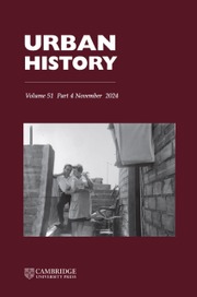
Most of the map sheets of the urban cadastre of Rome feature errors of measurement greater than is generally acceptable today. The GIS techniques of calibration, georeferencing and the transformation of projection overcome most of the problems of accuracy by reducing the distortion of the paper format, the imprecision of the measuring techniques and the lack of a projection system. The 94 sheets of the urban cadastre of Rome were georeferenced using a network of ground control points (GCPs) based on a custom-made GPS survey, and then digitized (Figure 3).Footnote ²⁴

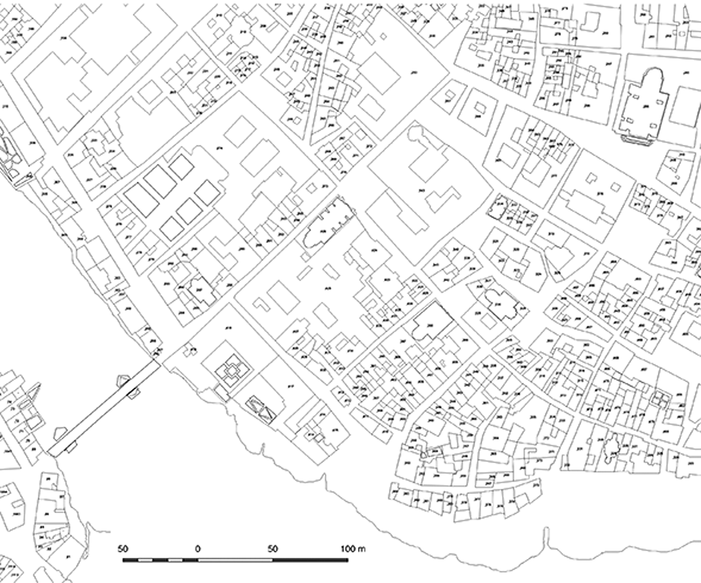
Source: urban cadastre of Rome, 1818–24.

Figure 3. Digital map of urban cadastre of Rome, rione Regola, fragment

Thematic information was collected from the second series of brogliardi. The complex inter-dependencies, especially those observable amongst owners and property types, were handled in relational databases so as to avoid duplication. The brogliardi is configured as a list of real estate units (fondi) with their characteristics, estimate values (estimi) and respective owners (proprietary). It was possible to interpret this source so as to retrieve consistent information about:

• the property types: private property of an individual person or shared (multiple properties), property of public or religious authority;
• the social status of the owners: aristocratic, bourgeois, ecclesiastical, public administrator and so on;
• the property use: housing, economic activities, public offices, education, cultural and so on;
• the physical characteristics of the units: number of floors, number of rooms.

Notwithstanding the difficulties arising from the complexity of relationships and the frequent inconsistencies in reporting estimated values, it was decided to include them in the dataset, after having introduced a series of quality controls. Operationally, the information obtained from the second brogliardi was classified according to the above-listed categories and associated with polygons representing single cadastral parcels through ad hoc data querying routines.Footnote ²⁵ Thus, it was possible to produce new quantitative information which facilitated statistical analysis and thematic mapping of different socio-economic characteristics of 1820s Rome within the Aurelian Walls. Information was aggregated from the parcel level to the city block and district levels so as to compare various performance indexes easily. The following thematic maps were produced: building consistency, land uses, property types, social status of owners, estimated property values.

The distribution of parcels, owners and properties amongst the districts (rioni) of Rome is summarized in Table 1. Pronounced dissimilarities characterize different districts, reflecting the variability of the urban structure and its stratification. Simple thematic maps clearly illustrate spatial distributions of physical characteristics derived from the cadastral source. Building density (percentage of built-up area/total district area) is high in the bends of the River Tiber, an area that was densely built on during the Middle Ages but had been inhabited since antiquity (Ponte, Parione, Regola, S. Eustachio and Pigna districts). The north-eastern districts (Trevi, Colonna, Campo Marzio) and rione Borgo have slightly lower building densities, while the large peripheral districts (Trestevere, Ripa, Campitelli, Monti), characterized by the presence of villas, gardens and vineyards, have fairly low building density indexes (Figure 4).

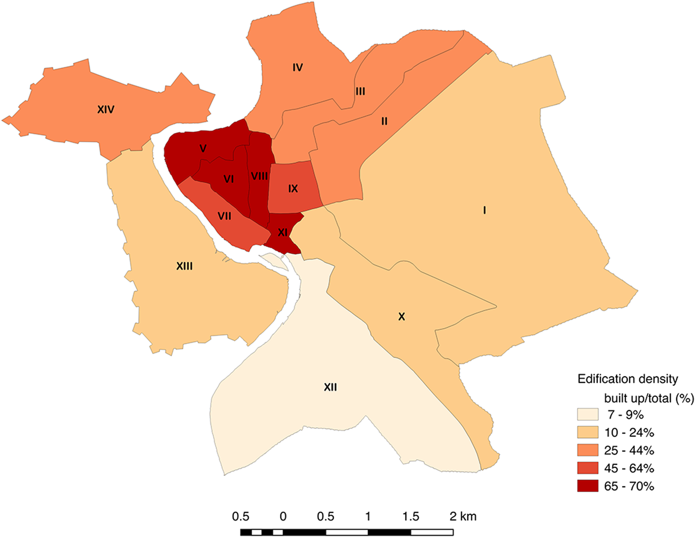
Source: urban cadastre of Rome, 1818–24.

Figure 4. Building density in the Roman districts

Table 1. Distribution of owners and properties

Source: urban cadastre of Rome, 1818–24.

The difference between the medieval and the baroque city is evident from the inspection of the property values (estimates) in Figure 5. The mapped index represents a normalized ratio of the sum of estimated property values and the total number of owners per district. The highest property values are to be found close to the main political and administrative poles, in the areas of Montecitorio (Curia Innocenziana, Ospizio Apostolico) and Quirinale (Palazzo Pontificio nel Quirinale, Dataria Apostolica, Consulta) respectively to the left (west) and to the right (east) of Via del Corso. Around these two power zones, imposing residences as well as new commercial buildings, and buildings associated with welfare and production, were built between the seventeenth and the eighteenth centuries. These dynamics are reflected by the property values, which are higher in the central districts of Parione, Pigna, Colonna and Trevi. With reference to the property type, the brogliardi registers indicate that, on average, 54 per cent of owners fell into the category of ‘single private’. This feature is more pronounced in the districts of Trevi, Colonna, Campitelli and S. Eustachio. Multiple occupancy properties made up, on average, 17 per cent of the total, with higher shares in the districts of Regola, Colonna and Campo Marzio and lower shares in Pigna, S. Angelo and Campitelli. Property held by public authorities or religious bodies averaged 28 per cent of the total, with a stronger presence in Borgo, the heart of ecclesiastical Rome, as well as in Monti and Trastevere, where the number of convents and monasteries situated in the green suburbs was higher than in other parts of the city (Figure 6). The distribution of owners according to social status shows the prevalence of a bourgeois element, averaging 48 per cent of all owners across the city, with higher shares in the districts of Colonna, Parione and Regola. Aristocratic owners (averaging 18 per cent) had a stronger presence in the districts of Trevi, Campitelli, S. Eustachio, Pigna and Ponte, while the ecclesiastical category accounted for 17 per cent of the total number of owners, and was more numerous in Monti, Pigna and Parione. The class of owners termed ‘Other’ represents mostly public administration and foundations, except for the S. Angelo district where, due to the presence of the walled Ghetto, Jewish people were forced to live in extremely overcrowded conditions (Figure 7).

Source: urban cadastre of Rome, 1818–24.

Figure 5. Average property values per owner in the Roman districts

Source: urban cadastre of Rome, 1818–24.

Figure 6. Property type in the Roman districts

Source: urban cadastre of Rome, 1818–24.

Figure 7. Ownership structure in the Roman districts

Exploring spatial relationships

Summary statistics at the district level are useful for carrying out both synchronic and diachronic analyses, but they do not account for large-scale spatial distributions. The organization of thematic information at the parcel level enables an in-depth analysis of the urban structure to be undertaken. Parcel detail is analysed here by considering the difference between the number of real estate units and the number of owners (Figure 8). More than 70 per cent of the parcels were characterized by a difference equal to 0. Negative values, indicating the presence of multiple occupancy properties do not appear clustered throughout the city, except for the previously mentioned Jewish ghetto, where the distribution of values was associated with the presence of Jus Gazagà, the right of perpetual use of properties granted to Jewish families.

Source: urban cadastre of Rome, 1818–24.

Figure 8. Difference between the number of real estate units and the number of owners per parcel, fragment

Positive values of the difference amongst the number of real estate units and the number of owners in each parcel show a spatial distribution apparently related to social status. ‘More’ properties by a single owner in a single parcel often indicated the presence of aristocratic or ecclesiastical social class in that parcel. If we compare the distribution of parcels with positive values in Figure 8 to the distribution of properties belonging to the aristocracy in Figure 9, a correspondence is noticeable in the densely built-up and highly stratified urban area along Via Papalis, the procession path used to connect the Cathedral of Rome (Basilica San Giovanni in Laterano) to the Vatican City. However, there is no correspondence between the ownership structure and the fragmentation of property units along the north–south axis unfolding along Via del Corso, where the aristocratic palaces were characterized by a unitary structure. In Figures 8 and 9 spatial distributions appear complex and difficult to grasp because of the large-scale cartographic representation. At this level of detail, geostatistics can help to identify underlying trends and behaviours and to explore the relationships amongst variables.

Source: urban cadastre of Rome, 1818–24.

Figure 9. Properties by aristocratic owners, fragment

The spatial distribution of a variable can be random, dispersed or concentrated. The last two distributions indicate the presence of spatial interdependence, also called spatial autocorrelation. We analyse the spatial distribution of selected variables aggregated per cadastral unit (parcel).Footnote ²⁶ These variables are: number of rooms; number of bourgeois, aristocratic and ecclesiastical owners; total property values (sum of estimated property values per parcel). We observe the presence of statistically significant positive spatial autocorrelation, meaning that spatial distributions are neither random nor dispersed, but clustered. Spatial clusters occur when similar, high values of variables are observed in adjacent spatial units (parcels). The detailed test statistic for spatial autocorrelation is reported in the Appendix.

In Figure 10, we can observe the presence of spatial clusters for a number of variables and compare different distributions. Large clusters in the city's green belt are characteristic of ecclesiastical ownership. Convents and monasteries were traditionally located at a certain distance from the built-up area of the city, surrounded by gardens and vineyards necessary for their food supply. Another characteristic of ecclesiastical ownership was the random distribution throughout the built-up area of the city, determined by the diffused and highly diversified presence of ecclesiastical real estate properties. For this reason, there are only a few significant clusters of ecclesiastical ownership in the central area. These are close to the strongholds of ecclesiastical power (Curia Innocenziana, Palazzo del S. Officio) and in foreign ecclesiastical institutions such as colleges, hospices or hospitals (Figure 10a).

Source: urban cadastre of Rome, 1818–24.

Figure 10. Spatial clusters for ownership types and estimate values

The spatial distribution of bourgeois ownership was far from homogeneous, reflecting the complexity and fragmentary nature of the property structure. Thus, it is almost impossible to find significant clusters for this ownership class. However, concentrations of bourgeois ownership along the axis Via del Babuino-Via Felice, situated on the edge of the compact city to the east, should be noted. This area was urbanized during the sixteenth century, after the interventions in the road system undertaken by Pope Sisto V (Figure 10b).

Aristocratic owners were clustered in well-defined areas both in the city centre and in the green belt (Figure 10c). These areas correspond to concentrations of noble palaces and suburban villas and with the detailed mapping of properties by aristocratic owners in Figure 9. Since aristocrats tended to exclude co-presence with other social classes, clusters ‘host’ a significant part of the total aristocratic ownership.

Spatial clusters of aristocratic owners show similar distribution patterns to those of estimated property values (estimates) in different parts of the city. Estimates were characterized by a stronger spatial autocorrelation and were concentrated along the axis of Via del Corso, around Piazza San Marco (today's Piazza Venezia), Piazza Navona, Piazza Farnese and Piazza Borghese (Figure 10d). These locations were the sites of prestigious buildings, ranging from noble to administrative palaces, schools and academies, churches and so on.Footnote ²⁷ It is interesting to notice the infrequency of high property values in the densely built-up bends of the River Tiber, along the ancient and medieval paths leading towards S. Angelo Bridge and the Vatican. In this region, the building consistency is the highest in Rome but secular stratification and continuous property transformations prevented the formation of ownership-based clustering. In this area, the only clustered variable from those selected is the number of rooms per parcel, not shown amongst the maps but analysed in Table 2 in the Appendix.

Table 2. Global Moran's I, distribution of spatial units in the quadrants of the Moran scatterplot according to local indicators of spatial association (LISA) and to the significance levels. LISA statistic is expressed as a percentage of the total significant units. Significance levels are expressed as a percentage of the total number of spatial units.

It emerges from the analysis above that the aristocracy were more likely to be found in clusters compared to other ownership classes. Also, according to the brogliardi, the highest property values were associated with this aristocratic social class. Therefore, it appeared reasonable to deepen the study on possible relationships between the aristocratic presence and the property structure and physical characteristics, by estimating a regression model reported in detail in the Appendix. We found that the number of aristocratic owners per parcel is strongly and positively related to the presence of private single owners, and thus to the property type. Variables representing property characteristics of the urban space such as fragmentation (number of real estate units per parcel), building consistency (number of rooms per parcel), building quality (estimated property values), despite being highly significant, were, surprisingly, less influential statistically.

Final remarks

GIS and geostatistics offer powerful opportunities for the analysis of data sources and communication of research in urban history. GIS tools provide effective solutions for overcoming problems and limitations related to the imprecise, incomplete and fragmentary nature of historical sources and for jointly managing, interrogating and visualizing multiple levels of information. The analytical power of a historical GIS can be enhanced with the use of geostatistics. These methods – to be found in the toolbox of scholars from other disciplines, such as economists, earth scientists or geographers – offer wider insights on complex spatial relationships.

The analysis of the nineteenth-century urban cadastre of Rome increased the level of knowledge about the historical city by producing and making available to historians of different disciplines detailed information about the physical and socio-economic characteristics of the urban space. New thematic layers were identified depicting the whole city, including land uses, building heights and building consistency, property types and property values and social status of the owners, and the spatial relationships amongst these layers were closely investigated. Different social classes had diversified spatial behaviours: the nobles tended to cluster in central areas close to hotspots of political power; the clergy clustered mainly in the outskirts; while the bourgeois did not demonstrate obvious clustering patterns. These findings can be considered as valuable starting points for future studies on contemporary Rome, as well as helping to further methodological investigations on the use of geostatistics and econometrics in urban historical studies.

The above-illustrated work is part of the project ‘The Historical Atlas of Rome’ promoted by CROMA – University Roma Tre. The strong multidisciplinary nature of the project encouraged the participation of urban historians from different areas with different research interests. The step-by-step implementation of the Atlas has received excellent feedback from researchers working in the fields of demography, archaeology, economy and art history. The ambitious long-term objective is to make available a dynamic web-based multithematic and multitemporal spatial database. A first step towards the achievement of this objective was the release in 2017 of the historical Web-GIS of Rome, with detailed information about the eighteenth-century city. Layers of information from the nineteenth century will be added to the platform in the near future. The Web-GIS supports large and differentiated data sources to be integrated within the digital cartography. The structure of the cadastre can host information from other historical databases, provided they can be linked to the cartographic base. Some experimenting has been done with the database of the stati delle anime (register of the population held by the parishes) that could be integrated into the cadastral maps for the years covered by the second brogliardi, adding precious information on demography. Other sources to be integrated within the GIS system are the post-Unitarian cadastral updates (post-1870) and the building licences database of the nineteenth century, that would allow for an entirely new range of thematic comparative studies on modern Rome.

Appendix: statistical evidence

The presence of spatial autocorrelation is verified by performing the Moran's I test statistic, which measures the global autocorrelation of each variable.Footnote ²⁸ Moran's I is generally presented as a standardized measure which, when the number of observations is large enough, is distributed as a standard normal. Moran's I values range from -1 to +1, with values close to 0 indicating the lack of spatial autocorrelation. Values close to 0 of the Moran's I will not reject the null hypothesis of spatial randomness, while positive (or negative) values close to 1 will indicate the presence of significant positive (or negative) spatial autocorrelation.

The other test is LISA statistics,Footnote ²⁹ which returns a measure of spatial autocorrelation for each individual location in relation to its neighbours and provides information about which unit values are statistically significant compared to spatial randomness.Footnote ³⁰ Spatial autocorrelation can be positive or negative. High values of one variable observed in one location, associated to high values of the same variable observed in adjacent locations (HH) are positive relationships, also identified as ‘hot spots’ or clusters, since they indicate the tendency of a variable to concentrate in space in particular locations. Low values observed in one location, associated to low values observed in adjacent locations (LL) are positive relationships as well, showing the tendency of a variable toward spatial dispersion. Negative spatial autocorrelation occurs when high values observed in one location are associated to low values observed in adjacent locations (HL), or vice-versa (LH). These types of observations are also called outliers, generally indicating anomalous spatial behaviours or data errors.

The results of Global Moran's I and LISA test statistics for the previously illustrated variables are reported in Table 2. Positive values of the Global Moran's I indicate the presence of positive spatial autocorrelation – meaning that spatial distributions are neither random nor dispersed – for all the chosen variables. This spatial behaviour is more evident for the variables ‘number of rooms’ and ‘estimate values’, which describe building characteristics. Spatial distributions according to social class are less ‘powerful’, but in the case of aristocratic owners the index value is higher.

The columns referring to LISA statistic show a strong presence of spatial units characterized by positive spatial association (HH), indicating potential clustering of high values (‘hot spots’) for all the variables, and of low values (LL or ‘cold spots’) only for the number of rooms and for the presence of owners from the bourgeois and aristocratic social class. The strong presence of spatial units both in the high–high and low–low spatial relationship class is a proof of accentuated homogeneity in the spatial behaviour of some variables. This is an obvious behaviour for the number of rooms per parcel, where hot spots are expected to be in the city centre and cold spots in the green belt, but is less obvious in the cases of ownerships related to social class. In Rome, the number of bourgeois and aristocratic owners per parcel tend to be clustered both for high and low values. Spatial outliers of the type low–high (LH) or high–low (HL) are more present for the variables ‘estimate values’ and ‘ecclesiastical owners’. This is justifiable for variables characterized by a high variability and inhomogeneity of their spatial distribution. For example, it is possible to comment on the elevated number of spatial outliers for the ecclesiastical owners in terms of ‘scattered’ presence of properties across the city and highly differentiated property types (ranging from the small flats in the city centre, to gardens and vineyards in the green belt, to palaces, monasteries, churches and so on).

The share of statistically insignificant units (column ‘Not significant’ in Table 2) is relatively high for all the variables, which means that a large number of parcels is to be excluded from the cluster analysis. However, it is interesting to notice that the percentage of spatial units with significant p-values (column ‘High significance level’ in Table 2) is higher for the variables ‘number of rooms’, and ‘estimated property values’. These results, as already anticipated in exploring spatial relationships, indicate that building consistency and estimated property values are characterized by strong spatial autocorrelation and that aristocratic ownership shows a stronger tendency to cluster if compared to other ownership classes.

To investigate further the relationships amongst the aristocratic presence and the property structure and physical characteristics, we estimate an ordinary least squares regression model (OLS) where the dependent variable is the ‘number of aristocratic owners per parcel’ and the dependent variables are: estimate values, number of rooms, total number of owners, number of real estate units, number of multi-properties and number of single owners per parcel. The linear relationship is defined as follows:

(1)

$\eqalign{{\rm NOB} &= {\bi \beta} _ 1{\rm EST}+ {\bi \beta} _ 2{\rm RMS}\cr& \quad+ {\bi \beta} _ 3{\rm OWN}+ {\bi \beta} _ 4{\rm PROP}+ {\bi \beta} _ 5{\rm MUL}+ {\bi \beta} _ 6{\rm SING}+ \varepsilon}$

where ɛ is the error component, assumed to be homoscedastic, independent and identical through all the spatial units.

The OLS regression results, aimed at giving a first empirical evidence of variables that have a greater effect on the presence of aristocratic owners in the various spatial units, are reported in Table 3, column (a). These results indicate the presence of relevant relationships, but the coefficient of determination is quite low (adjusted R ² around 30 per cent), suggesting that the model needs to be corrected for spatial dependency, spatial error, or omitted variables.

Table 3. Model estimation

The presence of spatial autocorrelation was evaluated with the diagnostic Lagrange multiplier test statistic (LM), performed on OLS estimates residuals using the Moran's I statistic and applying a spatial structure in the form of a first order spatial weight matrix, defined exogenously by the Voronoi polygons originated around parcel centroids, which represent an arbitrary, instrumental delimitation of the spatial units. The LM test for the presence of spatial autocorrelation (spatial lag) resulted not significant, while the LM test for the presence of spatial autoregressive error (spatial error) was highly significant,Footnote ³¹ meaning that the assumption of homoscedasticity, independency and identical distribution across the observations for ɛ is violated and that the model needs to be corrected for the presence of spatially dependent omitted variables. Alternatively, it is possible to specify a first order autoregressive error term:

(2)

$$\varepsilon = \lambda {\rm W}\varepsilon + u$$

where W is the spatial weight matrix accounting for the reciprocal adjacency amongst the spatial units, λ is the spatial autoregressive error parameter and u is an uncorrected and homoscedastic error term.

Regression results, corrected for the presence of a spatial autoregressive error, are shown in Table 3, column (b). The adjusted R ² is around 40 per cent, indicating an improvement in the model robustness. The spatial error term (λ) has a positive effect and is highly significant. The signs of the control variables did not change with respect to the OLS specification in column (a), however, while controlling for spatial effects, some differences are observable in the magnitude and significance levels of some variables.

Regression results evidence the strong influence of the property type on the dependent variable, while the group of variables representing physical characteristics of property have less influence than expected. By observing the coefficient values in column (b) Table 3, we can easily calculate that an increment of 0.08 per cent in the number of single owners par parcel (around 10 per cent of the average value) is associated with a 0.019 per cent increment of aristocratic owners per parcel, which represents 7.5 per cent of their average number per parcel (0.26). Following the same logic, we learn that a 10 per cent increase in estimate values and number of rooms would result in a 1 per cent increment in the average number of nobles per parcel, while a 10 per cent increment in the number of real estate units per parcel would cause a decrease of 2 per cent in the average number of nobles per parcel. A negative relationship is observed also amongst the total number of owners and the number of nobles per parcel, but in this case the significance level is low (at p = 0.01).

It emerges from this analysis that the number of aristocratic owners per parcel is strongly and positively related to the presence of private single owners, and thus to the property type. Variables representing property characteristics of the urban space such as fragmentation (number of real estate units per parcel), building consistency (number of rooms per parcel), building quality (estimated property values), despite being highly significant, were, surprisingly, less influential statistically.

Supplementary material

The supplementary material for this article can be found at https://doi.org/10.1017/S0963926820000188.

Footnotes

Higher resolution, colour versions of the figures in this article can be viewed online as supplementary material. Follow the URL at the end of this article.

a) OLS; b) Spatial error model

Notes: Dependent variable is the number of aristocratic owners per parcel

Signif. Codes : 0 ‘***’ 0.001 ‘**’ 0.01 ‘*’ 0.05 ‘ 1

^□ Brogliardi registers report estimate values in tavole and centesimi

References

¹ Knowles, A.K., ‘Historical GIS: the spatial turn in social history’, Social Science History, 24 (2000), 451–70CrossRef Google Scholar; P. Doorn, ‘A spatial turn in history: using the combined space-time component’, GIM International (2005), www.gim-international.com/content/article/a-spatial-turn-in-history, accessed 8 Jan. 2019; Finnegan, D., ‘The spatial turn: geographical approaches in the history of science’, Journal of the History of Biology, 41 (2007), 369–88CrossRef Google Scholar; Powell, R., ‘Geographies of science: histories, localities, practices, futures, progress’, Human Geography, 31 (2007), 309–30CrossRef Google Scholar; Withers, C.W.J., ‘Place and the “spatial turn” in geography and in history’, Journal of the History of Ideas, 70 (2009), 637–58CrossRef Google Scholar.

² Gregory, I.N. and Ell, P.S., Historical GIS: Techniques, Methodologies and Scholarship (Cambridge, 2007)CrossRef Google Scholar; Gregory, I.N., Kemp, K. and Mostern, R., ‘Geographical information and historical research: current progress and future directions’, History and Computing, 13 (2001), 7–21CrossRef Google Scholar; Knowles, A.K., ‘Placing history: how GIS is changing historical scholarship’, in Hillier, A. (ed.), Digital Supplement, ESRI Press (Redlands, 2008)Google Scholar.

³ For examples of the use of HGIS at the national level see Gregory, I.N., ‘The Great Britain historical GIS’, Historical Geography, 33 (2005), 132–4Google Scholar; De Moor, M. and Wiedemann, T., ‘Reconstructing Belgian territorial units and hierarchies: an example from Belgium’, History and Computing, 13 (2001), 71–97CrossRef Google Scholar; Fitch, C.A. and Ruggles, S., ‘Building the national historical geographic information system’, Historical Methods, 36 (2003), 41–51CrossRef Google Scholar; McMaster, R.B. and Noble, P., ‘The USA national historical geographical information system’, Historical Geography, 33 (2005), 134–6Google Scholar; Merzlyakova, I.A., ‘Historical GIS initiative in Russia’, Historical Geography, 33 (2005), 147–9Google Scholar; Bol, P. and Ge, J., ‘China historical GIS’, Historical Geography, 33 (2005), 150–2Google Scholar; Kim, J.-H., ‘HGIS project of South Korea’, Historical Geography, 33 (2005), 152–4Google Scholar; Kunz, A., ‘Fusing time and space: the historical information system HGIS Germany’, International Journal of Humanities and Arts Computing, 1 (2007), 111–22CrossRef Google Scholar.

⁴ Examples of the use of HGIS at the urban level: Spence, C., London in the 1690s: A Social Atlas (London, 2000)Google Scholar; Orforda, S., Dorling, D., Mitchell, R., Shaw, M. and Smith, D., ‘Life and death of the people of London: a historical GIS of Charles Booth's inquiry’, Health Place, 8 (2002), 25–35CrossRef Google Scholar; Siebert, L., ‘Using GIS to document, visualize, and interpret Tokyo's spatial history’, Social Science History, 24 (2000), 537–74Google Scholar; Wilson, A., ‘Sydney timemap: integrating historical resources using GIS’, History and Computing, 13 (2001), 45–68CrossRef Google Scholar; Yano, K., Nakaya, T. and Isoda, Y. (eds.), Virtual Kyoto: Exploring the Past, Present and Future of Kyoto (Nakanishiya Kyoto, 2007)Google Scholar; Pinol, J.-L. and Garden, M., Atlas des Parisiens: de la Révolution à nos jours (Paris, 2009)Google Scholar; Novak, M.J. and Gilliland, J.A., ‘Trading places: a historical geography of retailing in London, Canada’, Social Science History, 35 (2011), 543–70Google Scholar; Lelo, K., ‘A GIS approach to urban history: Rome in the 18th century’, ISPRS International Journal of Geo-Information, 3 (2004), 1293–316CrossRef Google Scholar.

⁵ One of the first major achievements in associating quantitative analysis to digital mapping was the work on the cadastre of Carpi. See Bocchi, F. and Lugli, F., ‘Computer methods used to analyse and re-construct the cadastral map of the town of Carpi (1472)’, in Denley, P. and Hopkin, D. (eds.), History and Computing (Manchester, 1987), 222–7Google Scholar.

⁶ On the relevance of cadastral sources in Italy, see also Gambi, L., Una Geografia per la Storia (Turin, 1973)Google Scholar; Zangheri, R., ‘I catasti’, Storia d'Italia, vol. V (I documenti) (Turin, 1973), 761–806Google Scholar; Mattia, S. and Bianchi, R. (eds.), Forma e Struttura dei Catasti Antichi (Milan, 1994)Google Scholar; Longhi, A. (ed.), Catasti e Territori. L'analisi dei Catasti Storici per l'Interpretazione del Paesaggio e per il Governo del Territorio (Florence, 2008)Google Scholar.

⁷ Foglietti, R., ‘Il catasto di Macerata nell'anno 1268’, in Opusculi di storia del diritto (Macerata, 1886), 229–70Google Scholar; Carpentier, E., Orvieto à la fin du XIIIe siècle. Villes et campagnes dans le cadastre de 1292 (Paris, 1986)Google Scholar; Carocci, S., ‘Le comunalie di Orvieto fra la fine del XII e la metà del XIV secolo’, Mélanges de l'École française de Rome. Moyen-Âge, temps modernes, 99 (1987), 701–28CrossRef Google Scholar; Herlihy, D. and Klapisch-Zuber, C., Les Toscans et leurs familles. Une étude du catasto florentin de 1427 (Paris, 1978)Google Scholar.

⁸ Mazzucchelli, V., Catasto e volto urbano: Milano alla metà del settecento (Rome, 1983)Google Scholar; Romani, M., ‘Note sul patrimonio edilizio milanese intorno alla metà del settecento’, in Studi in onore di Armando Sapori, 2 vols. (Milan, 1957), vol. II, 1301–17Google Scholar; Zaninelli, S., Il nuovo censo dello stato di Milano dall'editto del 1718 al 1733 (Milan, 1963)Google Scholar.

⁹ Congé, A., ‘Le cadastre de Lombardie (1758): une source pour l'histoire urbaine. La réalisation d'un système d'information géographique pour la ville de Milan’, Città e Storia, 1 (2006), 457–78Google Scholar.

¹⁰ Fiscal, legal and property information contained in historical cadastres were traditionally used by rural historians for the study of landscapes and ownership distributions in the countryside. This usage is well reflected in the work of Zangheri, R., Catasti e storia della proprietà terriera (Turin, 1980)Google Scholar.

¹¹ Motu proprio of 6 July 1816, Reformatio publicæ administrationis et tribunalium ditionis pontificiæ. A useful reconstruction of all the institutional events is in Spagnuolo, V., I catasti generali dello Stato Pontificio. La cancelleria del censo di Roma poi agenzia delle imposte (1824–1830) (Rome, 1996)Google Scholar. See also Ruggeri, A. and Londei, L., ‘Il catasto urbano di Roma (1818–1824)’, in Cantile, A. (ed.), Eventi e documenti diacronici dele principali attività geotopografiche in Roma (Florence, 2000), 102–37Google Scholar; Spagnuolo, V., ‘Nuovi modelli organizzativi fra ancien régime, periodo napoleonico e Restaurazione: l'introduzione dei titolari d'archivio e la realizzazione del catasto gregoriano, Roma fra la restaurazione e l'elezione di Pio IX. Amministrazione, economia, società e cultura’, in Bonella, L., Pompeo, A. and Venzo, M.I. (eds.), Roma fra la Restaurazione e l'elezione di Pio IX (Rome, Fribourg and Vienna, 1997), 1–18Google Scholar.

¹² Chiachella, R., Richezza, nobiltà e potere in una provincia pontificia. La ‘Misura Generale del Territorio Perugino’ del 1727 (Perugia, 1996)Google Scholar; Chiachella, R., ‘I catasti dell'età moderna a Perugia’, Archivi per la Storia, 8 (1995), 193–215Google Scholar; Salterni, C. and Turra, D., ‘Il catasto Boncompagni e la documentazione catastale bolognese tra XVIII e XIX secolo’, Archivi per la Storia, 8 (1995), 257–66Google Scholar; Sinisi, D., ‘Catasti settecenteschi prima del catasto piano: catasti locali geometrico-parcellari e indirizzi politici dell'amministrazione centrale in materia catastale’, Archivi per la Storia, 8 (1995), 177–91Google Scholar.

¹³ For a reconstruction of the vicissitudes of pontifical finances and the debate on fiscal policies throughout the eighteenth century until the beginning of the nineteenth century, see Travaglini, C.M., ‘La proprietà immobiliare a Roma agli inizi del Settecento’, Archivi e Cultura, 28 (1995), 33–61Google Scholar; Travaglini, C.M., ‘Aspetti della modernizzazione economica tra fine settecento e inizi ottocento. La politica fiscale’, in Boutry, P., Pitocco, F. and Travaglini, C.M. (eds.), Roma negli anni di influenza e dominio francese 1798–1814. Rotture, continuità, innovazioni tra fine settecento e inizi ottocento (Naples, 2000), 233–72Google Scholar.

¹⁴ For an overview of innovations in urban cartographic representation, see Bevilacqua, M., ‘Catasti e rappresentazione della città nel settecento italiano’, Città e Storia, special issue published in the framework of the II Congress of the Italian Association of Urban History (2004), 31–8Google Scholar.

¹⁵ Spagnuolo, I catasti generali dello Stato Pontificio, 26.

¹⁶ Ibid., 41.

¹⁷ Ruggeri and Londei, ‘Il catasto urbano di Roma (1818–1824)’.

¹⁸ ‘Nuova Pianta / di / Roma / data in luce / da / Gianbattista Nolli / l'anno / MDCC XLVIII’ was the first geometrically correct bi-dimensional representation of the city of Rome, produced as a result of an accurate topographical campaign of measurements. For details on Nolli's work, see Bevilacqua, M., Roma nel secolo dei lumi. Architettura erudizione scienza nella pianta di G.B. Nolli ‘Celebre Geometra’ (Naples, 1998)Google Scholar. On the measurement techniques and the accuracy level of the Nolli map, see Lelo, K., ‘Nolli e la visione della città. Rigore ed estetica nella rappresentazione dello spazio urbano’, in Travaglini, C.M. and Lelo, K. (eds.), Roma nel settecento. Immagini e realtà di una capitale attraverso la pianta di G.B. Nolli (Rome, 2013), 3–42Google Scholar; Baiocchi, V. and Lelo, K., ‘Assessing the accuracy of historical maps of cities: methods and problems’, Città e Storia, 9 (2014), 61–89Google Scholar.

¹⁹ Archivio Storico Capitolino, Camerale II, Catasti, envelope 9.

²⁰ Two documentary series ‘Catastini’ and ‘Trasporti’ were created to record property variations. See Travaglini, C.M., ‘Le cadastre de Rome. De l'estime au cadastre en Europe. Les systèmes cadastraux aux XIXe et XXe siècles’, in Bourillon, F., Clergeot, P. and Vivier, N. (eds.), Colloque de 20 et 21 Janvier 2005 Comité pour l'histoire economique et financière de la France (Paris, 2008), 323–50Google Scholar.

²¹ The estimo was usually assigned to the owner and may include more real estate units (fondi), which do not necessarily lie within the same parcel.

²² Bultrini, S., Stemperini, G. and Travaglini, C.M., ‘Proprietà nobiliari e trasformazioni urbane a Roma: il caso di Piazza Navona (XVIII–XIX)’, in Botieux, M., Brice, C. and Travaglini, C.M. (eds.), Le Nobiltà delle città capitali (Rome, 2009), 181–258Google Scholar; Lelo, K. and Stemperini, G., ‘La dimensione economica nella città dell'Ottocento: un'analisi critica delle fonti fiscali e amministrative’, Città e Storia, 13 (2018), 103–15Google Scholar.

²³ Istruzioni per la rettifica catastale della parte topografica e descrittiva delle proprietà costrutte della provincia di Roma (Florence, 1871); Archivio di Stato di Roma, Presidenza del Censo, envelope 2105.

²⁴ Baiocchi, V. and Lelo, K., ‘Georeferencing the historical maps of Rome between the seventeenth and eighteenth centuries’, XX International CIPA Symposium International Cooperation to Save the World's Cultural Heritage (Turin, 2005)Google Scholar.

²⁵ The level of detail of brogliardi is greater than that of the cadastral maps: one parcel is composed of many real estate units (fondi) which have one or more owners. Thus, in order to map the information deduced from the brogliardi, it is necessary to aggregate data at the parcel level. Aggregated data is, by necessity, standardized according to specific rules; it may run the risk of losing the most peculiar characteristics and/or representative values. For further insight on methodological aspects, see Lelo, K., ‘GIS e storia urbana’, in Morelli, R., Sonnino, E. and Travaglini, C.M. (eds.), I territori di Roma, storie, popolazioni, geografie (Rome, 2002), 191–211Google Scholar; Lelo, K., ‘L'ambito urbano di piazza Navona: una interpretazione attraverso le fonti cartografiche e documentarie sette-ottocentesche’, in Bernard, J.-F. (ed.), Piazza Navona, ou Place Navone, la plus belle et la plus grande (Rome, 2014), 557–70Google Scholar.

²⁶ To account for spatial contiguity instead of using the parcel shapes, we use Voronoi polygons drawn around each parcel centroid, also known as Thiessen polygons. Aurenhammer, F., ‘Voronoi diagrams – a survey of a fundamental geometric data structure’, ACM Computing Surveys, 23 (1991), 345–405CrossRef Google Scholar.

²⁷ Brogliardi registers often lack information about estimated property values of churches.

²⁸ Moran's I is given by the following expression: $I = {\rm \;}{N \over S}\;{{\mathop \sum \nolimits_{ij}^N W_{ij}\lpar {X_i\;-\bar{X}} \rpar \lpar {X_j\;-\bar{X}} \rpar } \over {\mathop \sum \nolimits_{i = 1}^N {\lpar {X_i\;-\bar{X}} \rpar }^2}}$, where: x_i is the studiedvariable in region I; $\bar{x}$ is the average sample value; W_ij are binary spatial weights: value 1 is given to the spatial units within distance d from the geographic centroid of the spatial unit, and 0 to all other regions; N is the sample dimension. S = Σ_iΣW_ij. P.A.P. Moran, ‘Notes on continuous stochastic phenomena’, Biometrika, 37 (1950), 17–23.

²⁹ Anselin, L., ‘Local indicators of spatial association-LISA’, Geographical Analysis, 27 (1995), 93–115CrossRef Google Scholar.

³⁰ Observed spatial distributions are compared with a user-defined number of randomizations, in order to quantify the probability of rejecting the null hypothesis of spatial randomness (significance level).

³¹ The hypothesis that the spatial autoregressive error is not present (λ = 0) is rejected at the 0.0001% of significance level. On application of LM test statistic, see Anselin, L., ‘Spatial econometrics’, in Mills, T.C. and Patterson, K. (eds.), Palgrave Handbook of Econometrics, vol. I: Econometrics theory (Basingstoke, 2006), 901–41Google Scholar.