


INTRODUCTION
Archaeologists are making increasing demands of radiocarbon (14C) calibration. When the first internationally agreed high-precision 14C calibration curve was issued (Pearson and Stuiver Reference Pearson and Stuiver1986; Stuiver and Pearson Reference Stuiver and Pearson1986), the median quoted error of 14C ages obtained by archaeologists was ca. 80 BP (Bayliss Reference Bayliss and Bayley1998: figure 11.9) and calibration of single samples was almost all that was attempted (e.g. Pearson Reference Pearson1987). Over the intervening decades the advent of accelerator mass spectrometry (AMS) means that archaeologists have been able to adopt more rigorous sampling protocols and obtain an increased number of age determinations for their sites (Ashmore Reference Ashmore1999), quoted errors on 14C measurements from archaeological samples have steadily reduced (e.g. Bayliss Reference Bayliss, Riddler, Soulat and Keys2016: figure 1), and formal chronological modeling of series of radiocarbon dates has become common practice (Bayliss Reference Bayliss2015: figure 1).

Figure 1 Density of tree-ring data in IntCal20 (intra-laboratory replicates have been combined and multi-year blocks spread proportionately across their bandwidth).
The SWOT framework (strengths, weaknesses, opportunities, and threats analysis) is a straightforward strategic planning technique that is of value in focusing attention on key issues which affect our ability to achieve stated goals (Sarsby Reference Sarsby2016). In the case of the IntCal20 calibration curve, our aim is to produce robust and accurate chronologies that are of sufficient precision to address our archaeological questions, such as the timings of construction and use of a series of Neolithic long barrows in central-southern England. Calendrical accuracy is of particular importance in the portion of the curve which is based on tree rings as it is in this period that 14C-based chronologies for archaeological remains are interpreted within historical frameworks and those based on dendrochronology. A series of new measurements obtained on single tree rings from a post that had previously been dated by ring-width dendrochronology from Lancaster Castle, UK, allow us to examine the precision and accuracy of wiggle-matching (Christen and Litton Reference Christen and Litton1995) timbers from historic buildings.
Data Coverage, Density, and Resolution
IntCal20 includes 9211 measurements on tree-ring samples whose calendar dates are known by dendrochronology, and a further 1498 measurements on samples from trees that have been tied to this sequence by radiocarbon wiggle-matching. Once intra-laboratory replicates have been combined (see below), there are 7946 results on known-age tree-ring samples and 1299 on wiggle-matched samples (Reimer et al. Reference Reimer, Austin, Bard, Bayliss, Blackwell, Bronk Ramsey, Butzin, Cheng, Edwards, Friedrich, Grootes, Guilderson, Hajdas, Heaton, Hogg, Hughen, Kromer, Manning, Muscheler, Palmer, Pearson, van der Plicht, Reimer, Richards, Scott, Southon, Turney, Wacker, Adolphi, Büntgen, Capano, Fahrni, Fogtmann-Schultz, Friedrich, Kudsk, Miyake, Olsen, Reinig, Sakamoto, Sookdeo and Talamo2020 in this issue). The comparable totals for IntCal13 were 3527 results on known-age samples and 232 results on wiggle-matched samples. This more than doubling of the quantity of data included in the new calibration curve is its first strength.
The known-age tree rings in IntCal20 run from 0 cal BP (AD 1950)Footnote 1 to 12,308 cal BP (10,359 BC), and the wiggle-matched tree rings run from 12,293 ± 4 cal BP (10,344 ± 4 BC)Footnote 2 to 14,194 ± 4 cal BP (12,245 ± 4 BC)Footnote 3, Footnote 4. These results are not spread evenly across this time period, however (Figure 1), with the density of data varying from an average of 2.7 measurements per year in the most recent millennium to only 0.2 measurements per year in the millennia from 9000–10,999 cal BP (7051–9050 BC). Three quarters of the data are concentrated in five of the fourteen millennia covered by the tree-ring-based part of IntCal20 (i.e. the most recent four millennia, and 12,000–12,999 cal BP [10,051–11,050 BC]). In the 8000 years between 4000 and 12,000 cal BP (2051–10,051 BC), IntCal20 includes just 303 new measurements that were not included in IntCal13. This variability in the density of data coverage is a weakness of the new calibration curve.
Over half of the tree-ring samples included in IntCal20 comprised single growth-rings (Figure 2), with a further 18% being blocks containing 2–5 rings. Single-year measurements are available for 2731 years (ca. 19% of the tree-ring-based part of IntCal20). Almost everywhere where high-resolution data are available, additional structure in the calibration curve has been revealed (for example, Figure 3). On the basis of the three 21-year blocks selected for the recent annual tree-ring inter-comparison, this additional structure can be expected usually to lie within, or very close to, the existing IntCal 1σ uncertainty envelope, although this may not always be the case (Wacker et al. Reference Wacker, Scott, Bayliss, Brown, Bard, Bollhalder, Friedrich, Capano, Cherkinsky, Chivall, Culleton, Dee, Friedrich, Hodgins, Hogg, Kennett, Knowles, Kuitems, Lange, Miyake, Nadeau, Nakamura, Naysmith, Olsen, Omori, Petchey, Philippsen, Bronk Ramsey, Prasad, Seiler, Southon, Staff and Tuna2020 in this issue: figure 1). The proportion of decadal and bi-decadal blocks in IntCal20 has reduced to 20% and 6% of the dataset respectively, but these are still the only data available for the majority of the tree-ring timescale.
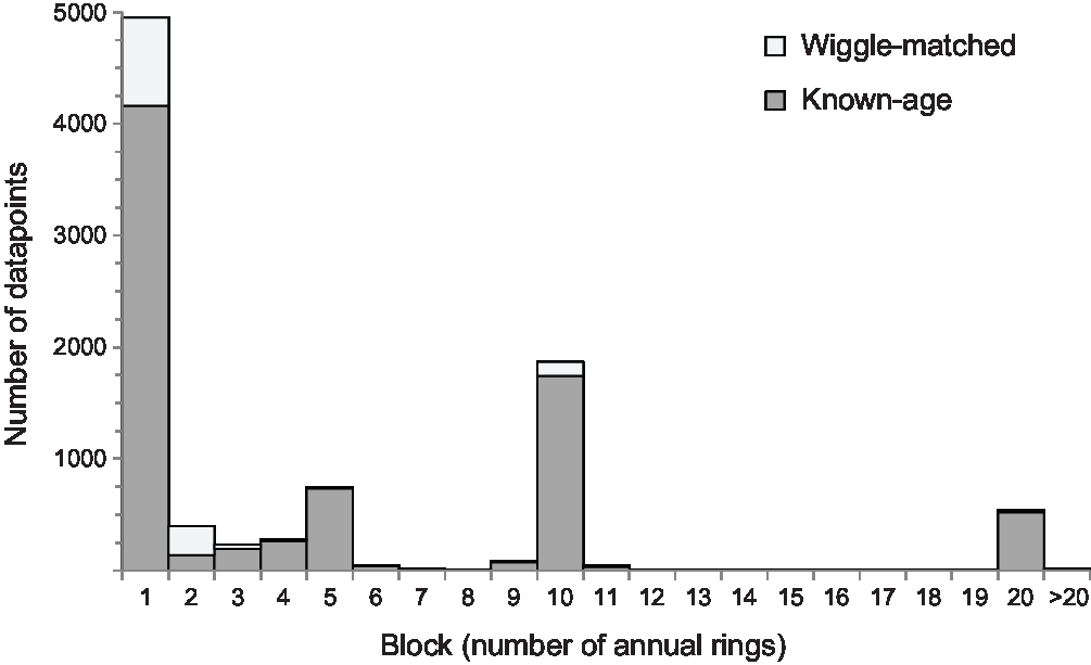
Figure 2 Resolution of tree-ring samples included in IntCal20 (intra-laboratory replicates have been combined).

Figure 3 Comparison of IntCal20 (dark grey) and IntCal13 (red) for the 250-year period from AD 950−1200 (1000–750 cal BP) showing the radiocarbon measurements from Lancaster Castle (LAN-C07), error bars and envelopes at 1σ.
For archaeologists, striving to create prehistories on a generational timescale, these data can be worryingly sparse. For example, for two generations in the later part of the 53rd century BC (5261–5210 BC; 7210–7160 cal BP), a gap in the decadal dataset from Seattle (QL, set 1, division 14 in the IntCal20 databaseFootnote 5 [hereafter e.g. 1-14]) means that the curve rests on just four measurements from Belfast on bi-decadal blocks (UB, 2-3 & 2-5) and two measurements from Heidelberg on a 4-year and a 5-year block (Hd, 5-5; Figure 4). This is an average data density of 0.1 measurements per year (the average density across the extent of the curve illustrated in Figure 4 is 0.2 measurements per year). This stands in contrast to some of the sites which are modeled against this part of the curve. For example, if the modeling for the chronology of the settlement at Versend-Gilencsa, Hungary is to be believed (Jakucs et al. Reference Jakucs, Oross, Bánffy, Voicsek, Dunbar, Reimer, Bayliss, Marshall and Whittle2018: figures 5 and 8), the data density for this archaeological settlement is at least double, and probably 20 times, that of the IntCal calibration curve against which it has been modeled. At a key juncture in European prehistory, as we try to understand the process by which Neolithic lifeways spread west and north out of the Danube corridor (e.g. Jakucs et al. Reference Jakucs, Bánffy, Oross, Voicsek, Bronk Ramsey, Dunbar, Kromer, Bayliss, Hofmann, Marshall and Whittle2016; Whittle et al. Reference Whittle, Bayliss, Barclay, Gaydarska, Bánffy, Borić, Draşovean, Jakucs, Marić, Orton, Tasić, Schier and Vander Linden2016; Denaire et al. Reference Denaire, Lefranc, Wahl, Bronk Ramsey, Dunbar, Goslar, Bayliss, Beavan, Bickle and Whittle2017; Meadows et al. Reference Meadows, Müller-Scheeßel, Cheben, Agerskov Rose and Furholt2019), this is clearly unsatisfactory.

Figure 4 Data density of IntCal20 between 5400 BC and 4900 BC (7349–6849 cal BP), showing paucity of data in the mid- and late 53rd century BC), error bars at 1σ.
The IntCal20 tree-ring data have been produced by 20 radiocarbon laboratories (Figure 5), with 60% produced by accelerator mass spectrometry (AMS), 31% by gas proportional counting (GPC), and the remaining 9% by liquid scintillation spectrometry (LSS). This is a marked change from the IntCal13 data, which was produced by eight laboratories with 80% of measurements made by GPC and only 1% by AMS. After application of error multipliers for the legacy data where appropriate (Stuiver et al. Reference Stuiver, Reimer, Bard, Beck, Burr, Hughen, Kromer, McCormac, van der Plicht and Spurk1998a: 1044–1045), the mean quoted estimates of total error produced by the three techniques in the IntCal20 dataset are equivalent: 19 ± 6 BP (AMS), 23 ± 9 BP (GPC), and 23 ± 6 BP (LSS).

Figure 5 Number of tree-ring samples in IntCal20 dated by each laboratory.
In principle more data from a larger number of laboratories should, on the basis of the “wisdom of crowds” (Galton Reference Galton1907), more accurately reflect the true value of atmospheric radiocarbon at a particular time. But it is clear that the density of IntCal20 tree rings almost never rises above four measurements per year, and for almost 90% of their extent fail to reach a density of two results per year (Figure 1). In these circumstances, the accuracy of the curve is very much dependent on the accuracy of the new high-resolution datasets as, in periods where these exist, they will overwhelm the decadal and bidecadal data. IntCal20 contains 4952 measurements on single-year samples (4161 on trees dated by dendrochronology and 791 on wiggle-matched trees). These results cover 2731 years, and for 1473 of these (54%) only one single-ring measurement is available. For another 347 years (13%), measurements are available for single rings from more than one tree from a single laboratory, and for the remaining 911 years (33%) results are available on more than one tree from more than one laboratory. Over half of these (61%) are for years in the most recent millennium.
The substantial increase in the amount of tree-ring data in IntCal20 is clearly a strength of the new calibration curve. The higher resolution of much of these new data allows detailed understanding of the shape of the calibration curve that was previously hidden (e.g. Figure 3). It is not, however, an enhancement that is spread equally (Figure 1). For almost half the extent of the tree rings, there are almost no new data and so, not only is there likely to be more shape in the calibration curve lurking within and around the IntCal20 envelope that is currently invisible, but in places the data density underlying the calibration curve is less than that of many archaeological applications (e.g. Figure 4). This is clearly an ongoing weakness. Single-year data now cover 19% of the tree-ring timescale, but well over half of this is not replicated by other measurements of a similar resolution, making the accuracy of IntCal20 vulnerable to any inaccuracy in these data.
Laboratory Replication
Not all the measurements on tree-ring samples reported in the IntCal20 database are on different samples, as some have been measured more than once. Four different kinds of replication have been reported in the dataset:
a. replicate measurements by a single laboratory on a single cellulose preparation (n = 973);
b. replicate measurements by more than one laboratory on a single cellulose preparation (n=13);
c. whole-process replicate measurements on the same tree-ring (or block of more than one tree ring) by a single laboratory (n=339);
d. whole-process replicate measurements on the same tree-ring (or block) by more than one laboratory (n=252).
Same-cellulose, same-laboratory replicates (i.e. replicate type a) above) have been reported by three laboratories: QL- (set 1, n=446), AIX- (set 61, n=23), and ETH- (set 69, n=504). These measurements have been combined before further analysis. In the case of the replicate groups produced by QL-, a weighted mean has been taken (Ward and Wilson Reference Ward and Wilson1978) before application of the error multiplier (1.3; Stuiver et al. Reference Stuiver, Reimer, Bard, Beck, Burr, Hughen, Kromer, McCormac, van der Plicht and Spurk1998a: 1044–1045); for ETH and AIX data the cellulose processing uncertainty (1‰ in Δ14C, or equivalently 8 BP in radiocarbon age) was removed from each replicate measurement in quadrature, and a weighted mean of the replicate ages (with corresponding uncertainty) was then calculated, before the cellulose processing uncertainty was finally added back in quadrature (Reimer et al. Reference Reimer, Austin, Bard, Bayliss, Blackwell, Bronk Ramsey, Butzin, Cheng, Edwards, Friedrich, Grootes, Guilderson, Hajdas, Heaton, Hogg, Hughen, Kromer, Manning, Muscheler, Palmer, Pearson, van der Plicht, Reimer, Richards, Scott, Southon, Turney, Wacker, Adolphi, Büntgen, Capano, Fahrni, Fogtmann-Schultz, Friedrich, Kudsk, Miyake, Olsen, Reinig, Sakamoto, Sookdeo and Talamo2020 in this issue). As these repeats form part of the protocols used by the laboratories to estimate their total laboratory error, they do not form an independent check on laboratory accuracy and so we do not consider them further here.
Replicate measurements on cellulose prepared in Arizona on single-rings from bristlecone pine 1971#059 were dated by three laboratories (i.e. replicate type b) above; STE-, 67-1, n=10; AA-, 68-9, n=11; ETH-, 69-51, n=16; Miyake et al. Reference Miyake, Jull, Panyushkina, Wacker, Salzer, Baisan, Lange, Cruz, Masuda and Nakamura2017). The differences between the measurements provided by the three laboratories are not statistically significant at the 5% level. They have not been combined before inclusion in IntCal20.
Ten laboratories have reported whole-process replicates on the same tree-ring or block of tree rings (i.e. replicate type c) above; Table 1). Following the application of the relevant error multiplier where appropriate (Stuiver et al. Reference Stuiver, Reimer, Bard, Beck, Burr, Hughen, Kromer, McCormac, van der Plicht and Spurk1998a: 1044–1045), 31 replicate groups (out of the 339) are statistically inconsistent at the 5% significance level. This is in line with statistical expectation.
Table 1 Whole-process intra-laboratory replicates on tree-ring samples reported for IntCal20 (*quoted errors are counting errors on samples and standards only (Stuiver Reference Stuiver1982: 5; Stuiver et al. Reference Stuiver, Kromer, Becker and Ferguson1986: 969); § these replicate groups were used in calculating the QL- radon offset (Stuiver et al. Reference Stuiver, Reimer and Braziunas1998b: 1128–1129); † earlywood/latewood replicates (Fogtmann-Schulz et al. Reference Fogtmann-Schulz, Østbø, Nielsen, Olsen, Karoff and Knudsen2017; Büntgen et al. Reference Büntgen, Wacker, Galván, Arnold, Arseneault, Baillie, Beer, Bernabei, Bleicher, Boswijk, Bräuning, Carrer, Ljungqvist, Cherubini, Christl, Christie, Clark, Cook, D’Arrigo, Davi, Eggertsson, Esper, Fowler, Gedalof, Gennaretti, Grießinger, Grissino-Mayer, Grudd, Gunnarson, Hantemirov, Herzig, Hessl, Heussner, Jull, Kukarskih, Kirdyanov, Kolář, Krusic, Kyncl, Lara, LeQuesne, Linderholm, Loader, Luckman, Miyake, Myglan, Nicolussi, Oppenheimer, Palmer, Panyushkina, Pederson, Rybníček, Schweingruber, Seim, Sigl, Churakova, Speer, Synal, Tegel, Treydte, Villalba, Wiles, Wilson, Winship, Wunder, Yang and Young2018).

Of the 20 samples where measurements have been reported separately on the earlywood and latewood of a single tree ring, two pairs of measurements from the same year on these two ring fractions are statistically inconsistent at the 5% significance level. This is no more than would be expected if these pairs were true replicates on exactly the same samples. While the difference between earlywood and latewood measurements in any particular year appears to vary not just in magnitude but also sign, the weighted mean difference in this dataset is 4.1 ± 5.1 BP (Figure 6). The samples included in IntCal20 come from across the AD 775 and AD 993 events, where the production of radiocarbon rapidly changed on an annual scale (Miyake et al. Reference Miyake, Nagaya, Masuda and Nakamura2012, Reference Miyake, Masuda and Nakamura2013). Thus any utilization of stored carbon from the previous years’ growth in earlywood (Kimak and Leuenberger Reference Kimak and Leuenberger2015) would be expected to be magnified in the radiocarbon signal in these trees, in comparison to those growing at times when the concentration of atmospheric radiocarbon was changing less rapidly. This finding is compatible with the suggestion, based on earlywood/latewood pairs from annual tree rings of a Danish oak dating from AD 1954–1970 that the radiocarbon in the earlywood originates from the actual growth year (Kudsk et al. Reference Kudsk, Olsen, Nielsen, Fogtmann-Schultz, Knudsen and Karoff2018). Two other recent studies report earlywood/latewood pairs on blocks of tree rings. McDonald et al. (Reference McDonald, Chivall, Miles and Bronk Ramsey2019: table 1) report six pairs on 5-year and 6-year blocks of English oak that have a weighted mean difference of 25.4 ± 15.3 BP, and Manning et al. (Reference Manning, Kromer, Cremaschi, Dee, Friedrich, Griggs and Hadden2020: table S1) report six pairs on decadal blocks of Swedish pine that have a weighted mean difference of 5.4 ± 8.2 BP. These differences are statistically indistinguishable (T′=1.8; T′(5%)=6.0; ν=1), and none is statistically significant.

Figure 6 Offsets between pairs of radiocarbon measurements on earlywood and latewood from the same annual tree ring (multiple results on different fractions of earlywood have been combined before this comparison), error bars at 1σ (divisions 62-4, 69-37, 69-38, and 69-40).
Whole-process replicate measurements from more than one laboratory are available on same-ring or same-block samples from 11 trees (i.e. replicate type d) above; Tables 2 and 3). Fourteen of the 356 replicate pairs in this dataset are statistically significantly different at the 5% significance level. This is fewer than would be expected on statistical grounds and may reflect a slight over-estimation of some reported errors (e.g. Pearson et al. Reference Pearson, Wacker, Bayliss, Brown, Salzer, Brewer, Bolllhalder, Boswijk and Hodgins2020 in this issue). The weighted mean differences between laboratories on single trees are generally 1–2‰ (8–16 BP; Tables 2 and 3). For Knet40, the AAR dataset (62-9) is significantly younger than the measurements from the three other laboratories on this tree (12.9 ± 3.1 BP; see Friedrich et al. Reference Friedrich, Kromer, Wacker, Olsen, Remmele, Lindauer, Land and Pearson2020 in this issue for further discussion). Laboratory offsets need not remain constant, however, and this finding relates to samples from a single tree measured in January 2019. From the IntCal20 data, we have limited evidence for the variability or stability of inter-laboratory offsets between measurements made at different times. The longest period over which we have inter-laboratory comparisons is for MAMS/ETH, where we have replicate measurements made between mid-2012 (Steinbach91) and the end of 2018 (Knet40). Over the course of these six years, the observed inter-laboratory offset does not appear to vary significantly (T′=3.5, T′(5%)=7.8, df=3; Table 3). In contrast the size of the offset between AA/OxA replicate measurements made on a Jordanian tree in 2014 is statistically significantly different (T′=12.0, T′(5%)=3.8, df=1; Table 3) from the size of the offset between AA/OxA replicate measurements made on another Jordanian tree in 2015. There are also replicate measurements available on non-identical blocks for Knet40 (Hd, 5-4), Cott418 (MAMS, 60-2 and ETH, 69-19), Brei232 (MAMS, 60-3 and ETH, 69-15), HKN-1 (GrA, 65-3 and PLD, 65-2), and Bamberg1, Blindheim37, Pettstadt48, and Vohberg34 (QL, 1-14 and PtA, 6-1), but overall there are replicate measurements from more than one laboratory on only 16 of the more than 500 trees represented in the IntCal20 dataset (ca. 3%).
Table 2 Whole-process inter-laboratory replicates on single tree rings from Knet40 included in IntCal20 (divisions 68-10, 62-9, 69-50, and 60-1; Friedrich et al. Reference Friedrich, Kromer, Wacker, Olsen, Remmele, Lindauer, Land and Pearson2020 in this issue); same-cellulose and intra-laboratory replicates have been combined: above diagonal = weighted mean difference, below diagonal = χ2red (degrees of freedom).
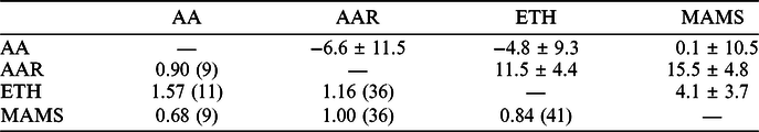
Table 3 Whole-process inter-laboratory replicates on same-blocks from same-trees included in IntCal20 (overall statistics include data from Knet40 (Table 2) where appropriate); † weighted mean differences are statistically significantly different (AA/OxA: T′=12.0: IAAA/PLD: T′=4.3; T′(5%)=3.8, df=1 for both).
The whole-process replicate measurements in the IntCal20 tree-ring dataset are valuable in demonstrating the reproducibility of the laboratories involved. This is another strength of the IntCal20 tree-ring dataset. Intra-laboratory replicates demonstrate that the laboratories involved reproduce within their quoted uncertainties. We note, however, that Table 1 includes measurements from only half of the laboratories who measured the tree rings in IntCal20, and only three laboratories (UCIAMS-, set 8, 42%; OxA-, divisions 63-15, 63-16, 63-17, and 59-1, 20%; and VERA-, set 64, 20%) have submitted whole-process replicates on more than 10% of the tree-ring samples they have dated. The inter-laboratory whole-process replicates are also valuable in demonstrating the reproducibility of measurements made in different laboratories, although some errors may be slightly over-estimated and inter-laboratory offsets generally fall between 1–2‰ (8–16 BP). Tables 2 and 3, however, include measurements from only seven laboratories, and only two laboratories (AA-, set 68, 27% and MAMS-, set 60, 24%) have inter-laboratory replicates on more than 10% of the samples they have dated. This variable, and generally low, replication rate means that our understanding of laboratory variability in IntCal20 is incomplete. Nonetheless, it is much better than our understanding of such variability in IntCal13, where the sample size required for conventional dating meant that very few whole-process or inter-laboratory replicates could be measured. Going forward, high-precision AMS presents opportunities for replication that were not available previously.
Variation in the Radiocarbon Content of Contemporary Tree Rings
An understanding of the intra- and inter-laboratory variation in measurement of the same sample is crucial because it enables differences in contemporary tree rings arising from laboratory variation to be distinguished from differences arising from other causes.
Some kinds of variation may be suspected on theoretical grounds but have not yet been unequivocally demonstrated in practice. These include potential variation in the radiocarbon content of contemporary trees from the same location, based on physiological factors such as the variable use of stored carbon from previous growing-seasons in earlywood, different species, or different environmental compartments. The IntCal20 tree-ring dataset includes little information on these issues. The earlywood/latewood replicates included in IntCal20 have been discussed above and are not statistically significantly different (Table 3), and there are measurements from ETH on contemporary single-rings from two timbers from a trackway at Timahoe West, Co. Kildare, Ireland (Q5653 (69-53) and Q6427 (69-49); 53.3N, 6.9W; Pearson et al. Reference Pearson, Wacker, Bayliss, Brown, Salzer, Brewer, Bolllhalder, Boswijk and Hodgins2020 in this issue). These have a weighted mean difference of 2.4 ± 7.1 BP, which is again not statistically significant.
It is also possible for atmospheric radiocarbon to vary locally for a variety of reasons, including the emission of depleted or 14C-free carbon from volcanic vents, ocean upwelling, variations in the seasonal extent of the Intertropical Convergence Zone (ITCZ), and anthropogenic sources (Hogg et al. Reference Hogg, Heaton, Ramsey, Boswijk, Palmer, Turney, Southon and Gumbley2019). Data which may be affected by these issues have deliberately not been included in IntCal20 (Reimer et al. Reference Reimer, Austin, Bard, Bayliss, Blackwell, Bronk Ramsey, Butzin, Cheng, Edwards, Friedrich, Grootes, Guilderson, Hajdas, Heaton, Hogg, Hughen, Kromer, Manning, Muscheler, Palmer, Pearson, van der Plicht, Reimer, Richards, Scott, Southon, Turney, Wacker, Adolphi, Büntgen, Capano, Fahrni, Fogtmann-Schultz, Friedrich, Kudsk, Miyake, Olsen, Reinig, Sakamoto, Sookdeo and Talamo2020 in this issue). Ocean upwelling has been suggested as a possible cause for the weighted mean difference (13.6 ± 6.2 BP) between datasets 1-1 (KI tree, 57.9N, 152.6W) and 1-4 (C tree, 48.1N, 124.4W) (Stuiver and Braziunas Reference Stuiver and Braziunas1998), and for the observed offsets between the IntCal data and measurements on Japanese tree rings (e.g. Nakamura et al. Reference Nakamura, Miyahara, Masuda, Menjo, Kuwana, Kimura, Okuno, Minami, Oda, Rakowski, Ohta, Ikeda and Niu2007). A small number of datasets have also been omitted from IntCal20 because they are within the ITCZ or on its boundary (e.g. Hua et al. Reference Hua, Barbetti, Zoppi, Fink, Watanasak and Jacobsen2004); and datasets suspected of incorporating fossil-fuel derived carbon from industry (e.g. Tans et al. Reference Tans, de Jong and Mook1979) have also been omitted.
Locational effects in the radiocarbon content of tree rings within a hemisphere have long been of concern for calibration (e.g. McCormac et al. Reference McCormac, Hogg, Higham, Lynch-Stieglitz, Broecker, Baillie, Palmer, Xiong, Pilcher, Brown and Hoper1998), but these are extremely difficult to demonstrate convincingly as they are of similar scale to the inter-laboratory differences observed in the IntCal20 dataset (Tables 2 and 3). Growing season (Kromer et al. Reference Kromer, Manning, Kuniholm, Newton, Spurk and Levin2001; Dee et al. Reference Dee, Brock, Harris, Ramsey, Shortland, Higham and Rowland2010; Manning et al. Reference Manning, Griggs, Lorentzen, Bronk Ramsey, Chivall, Jull and Lange2018, Reference Manning, Kromer, Cremaschi, Dee, Friedrich, Griggs and Hadden2020), altitudinal (Cain and Suess Reference Cain and Suess1976; Dellinger et al. Reference Dellinger, Kutschera, Nicolussi, Schießling, Steier and Maria Wild2004), and latitudinal (Büntgen et al. Reference Büntgen, Wacker, Galván, Arnold, Arseneault, Baillie, Beer, Bernabei, Bleicher, Boswijk, Bräuning, Carrer, Ljungqvist, Cherubini, Christl, Christie, Clark, Cook, D’Arrigo, Davi, Eggertsson, Esper, Fowler, Gedalof, Gennaretti, Grießinger, Grissino-Mayer, Grudd, Gunnarson, Hantemirov, Herzig, Hessl, Heussner, Jull, Kukarskih, Kirdyanov, Kolář, Krusic, Kyncl, Lara, LeQuesne, Linderholm, Loader, Luckman, Miyake, Myglan, Nicolussi, Oppenheimer, Palmer, Panyushkina, Pederson, Rybníček, Schweingruber, Seim, Sigl, Churakova, Speer, Synal, Tegel, Treydte, Villalba, Wiles, Wilson, Winship, Wunder, Yang and Young2018; Pearson et al. Reference Pearson, Wacker, Bayliss, Brown, Salzer, Brewer, Bolllhalder, Boswijk and Hodgins2020 in this issue) offsets have all been suggested, but most studies are confounded by potential inter-laboratory variation. For example, Manning et al. (Reference Manning, Griggs, Lorentzen, Bronk Ramsey, Chivall, Jull and Lange2018) identify a substantive and fluctuating offset between the 14C content of trees from Jordan (30.3N, 35.5E; 63-12–63-17) and IntCal13, which is both much reduced and less variable through time when the 14C results from the Jordanian junipers are compared with those from English oaks (Brehm et al. Reference Brehm, Bayliss, Christl, Synal, Adolphi, Beer, Muscheler, Solanki, Usoskin, Bleicher, Bollhalder, Tyers and Submittedsubmitted; 50.6N–53.2N, 4.2W–0.5W; 69-3, 69-7, 69-9, and 69-11; figure 7).

Figure 7 Comparison of 14C ages of Jordanian juniper made in Oxford (OxA; blue) and Arizona (AA; red; one significant outlier, AA-103300 (1081 ± 22 BP, for five-year block centered on AD 1885) is not shown), with IntCal13 (1σ envelope; blue curve; cf Manning et al. Reference Manning, Griggs, Lorentzen, Bronk Ramsey, Chivall, Jull and Lange2018: figure 2) and 14C ages on English oaks made in ETH Zürich (green).
Three studies avoid this issue. Using data measured at ETH Zürich only, Büntgen et al. (Reference Büntgen, Wacker, Galván, Arnold, Arseneault, Baillie, Beer, Bernabei, Bleicher, Boswijk, Bräuning, Carrer, Ljungqvist, Cherubini, Christl, Christie, Clark, Cook, D’Arrigo, Davi, Eggertsson, Esper, Fowler, Gedalof, Gennaretti, Grießinger, Grissino-Mayer, Grudd, Gunnarson, Hantemirov, Herzig, Hessl, Heussner, Jull, Kukarskih, Kirdyanov, Kolář, Krusic, Kyncl, Lara, LeQuesne, Linderholm, Loader, Luckman, Miyake, Myglan, Nicolussi, Oppenheimer, Palmer, Panyushkina, Pederson, Rybníček, Schweingruber, Seim, Sigl, Churakova, Speer, Synal, Tegel, Treydte, Villalba, Wiles, Wilson, Winship, Wunder, Yang and Young2018: figure 3) identify a weak meridional north–south gradient of declining average 14C values across the AD 770s and AD 990s, although there is considerable variation around this trend. A statistically significant average weighted mean difference of −8.1 ± 1.9 BP between Irish oak (53.3N, 6.9W; 68-4–6, 69-49 and 69-53–4) and bristlecone pine (37.5N, 118.2W; 68-1–3) has been been calculated taking into account inter-laboratory differences (Pearson et al. Reference Pearson, Wacker, Bayliss, Brown, Salzer, Brewer, Bolllhalder, Boswijk and Hodgins2020 in this issue). Data from the Heidelberg laboratory published by Manning et al. (Reference Manning, Kromer, Cremaschi, Dee, Friedrich, Griggs and Hadden2020: table S1) produce average weighted mean differences of 4.6 ± 3.3 BP between Irish oak (54.3−55.2N, 6.3−8.4W; 63-3) and Turkish pine (40.4N, 31.0E; Çatacık), and 4.4 ± 2.3 BP between German oak (48.1−49.5N, 9.8−12.1E; 63-8, 63-9, 63-10, 63-11) and the same Turkish pine. Kromer et al. (Reference Kromer, Manning, Kuniholm, Newton, Spurk and Levin2001: 2530) argue for a time-transgressive offset to older ages for the Turkish pine in the late fifteenth and early sixteenth centuries AD. However, this proposed offset is not seen consistently over other time periods and, taken as a whole, there is no evidence that the full sequence of observed differences between the measurements from the three locations are not solely independent random noise. A turning-point test for independence (Kendall Reference Kendall1973) on the time series of observed differences gives p-values of 0.33, 0.65, and 0.41 for the German–Irish, German–Turkish, and Irish–Turkish sets respectively. Consequently, it is difficult to distinguish whether these observed differences are due to locational effects as opposed to other potential sources of variation.
Further discussion of these issues is provided by Reimer et al. (Reference Reimer, Austin, Bard, Bayliss, Blackwell, Bronk Ramsey, Butzin, Cheng, Edwards, Friedrich, Grootes, Guilderson, Hajdas, Heaton, Hogg, Hughen, Kromer, Manning, Muscheler, Palmer, Pearson, van der Plicht, Reimer, Richards, Scott, Southon, Turney, Wacker, Adolphi, Büntgen, Capano, Fahrni, Fogtmann-Schultz, Friedrich, Kudsk, Miyake, Olsen, Reinig, Sakamoto, Sookdeo and Talamo2020 in this issue). Two points are of relevance here. First, that any locational variation in the radiocarbon content of contemporary tree rings within the IntCal20 dataset is likely to be of similar magnitude to the observed inter-laboratory variation within the dataset (Tables 2 and 3), and, secondly, that IntCal20 contains tree rings from a much wider range of locations than did IntCal13 (Reimer et al. Reference Reimer, Austin, Bard, Bayliss, Blackwell, Bronk Ramsey, Butzin, Cheng, Edwards, Friedrich, Grootes, Guilderson, Hajdas, Heaton, Hogg, Hughen, Kromer, Manning, Muscheler, Palmer, Pearson, van der Plicht, Reimer, Richards, Scott, Southon, Turney, Wacker, Adolphi, Büntgen, Capano, Fahrni, Fogtmann-Schultz, Friedrich, Kudsk, Miyake, Olsen, Reinig, Sakamoto, Sookdeo and Talamo2020 in this issue: figures 1 and 8). The calibration curve is still dominated, however, by trees that grew between 46°N and 55°N, which account for more than three-quarters of the dataset. In these circumstances, no attempt has been made to disentangle the various sources of variation between measurements on contemporary trees in IntCal20. Rather the curve is an estimation of the hemispherical average atmosphere and the quoted uncertainty on the curve encompasses the observed variation between contemporary trees within the IntCal20 dataset from all potential sources.

Figure 8 Latitude of tree-ring samples included in IntCal20.
It is important to note that any additional independent variation, beyond that reported by the laboratories, that is detected within the IntCal20 data is automatically incorporated into the construction of the IntCal20 calibration curve. If the measurements included in IntCal20 from the same calendar year appear more widely spread (overdispersed) than the laboratory reported uncertainties would suggest, this is propagated through curve construction and accounted for in subsequent predictive intervals. This is discussed in detail in Heaton et al. (Reference Heaton, Blaauw, Blackwell, Bronk Ramsey, Reimer and Scott2020 in this issue). This means that it should be possible to obtain accurate calibration of radiocarbon measurements from anywhere north of the ITCZ using IntCal20, as long as the locational and laboratory variation in the test dataset is managed adequately in the modeling process (e.g. Hogg et al. Reference Hogg, Heaton, Ramsey, Boswijk, Palmer, Turney, Southon and Gumbley2019: 1285–1287).
Dendrochronologies
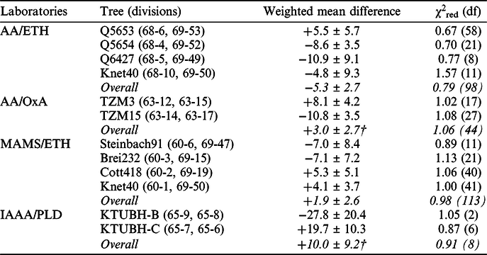
Almost half the tree-ring samples included in IntCal20 derive from the Hohenheim Holocene oak chronology (HOC), the Preboreal pine chronology (PPC) which cross-dates against it, or from floating pine sequences that have been wiggle-matched against the PPC (Figure 9; Friedrich et al. Reference Friedrich, Remmele, Kromer, Hofmann, Spurk, Felix Kaiser, Orcel and Küppers2004; Reinig et al. Reference Reinig, Nievergelt, Esper, Friedrich, Helle, Hellmann, Kromer, Morganti, Pauly, Sookdeo, Tegel, Treydte, Verstege, Wacker and Büntgen2018, Reference Reinig, Sookdeo, Esper, Friedrich, Guidobaldi, Helle, Kromer, Nievergelt, Pauly, Tegel, Treydte, Wacker and Büntgen2020 in this issue; Sookdeo et al. Reference Sookdeo, Kromer, Büntgen, Friedrich, Friedrich, Helle, Pauly, Nievergelt, Reinig, Treydte, Synal and Wacker2019 in this issue; Sookdeo et al. Reference Sookdeo, Kromer, Adolphi, Beer, Brehm, Büntgen, Christl, Eglinton, Friedrich, Guidobaldi, Helle, Nievergelt, Pauly, Reinig, Tegel, Treydte, Turney, Synal and Submittedsubmitted; Hogg et al. Reference Hogg, Southon, Turney, Palmer, Ramsey, Fenwick, Boswijk, Büntgen, Friedrich, Helle, Hughen, Jones, Kromer, Noronha, Reinig, Reynard, Staff and Wacker2016). Measurements on the independent Irish oak chronology (Brown et al. Reference Brown, Munro, Baillie and Pilcher1986) run to 7164 cal BP (5215 BC), but before this the Hohenheim-based chronologies stand alone, apart from a very few measurements on single-rings from bristlecone pine (Figure 10). Bristlecone pine has also been measured in the mid-4th millennium cal BP (mid-2nd millennium BC), but otherwise it is only in the most recent three millennia where tree rings from a range of sources have been analysed. European oak and pines constitute 77% of all the tree-ring samples in IntCal20, and European wood dominates everywhere bar the centuries around 2000 cal BP (1AD/1BC) where Japanese wood predominates.
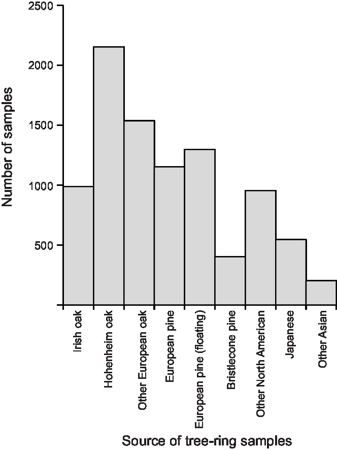
Figure 9 Source of tree-ring samples included in IntCal20.

Figure 10 Density of tree-ring samples in IntCal20 by source (intra-laboratory replicates have been combined and multi-year blocks spread proportionately across their bandwidth).
For 65% of the IntCal20 tree-ring samples, the raw data upon which the calendar age of the sample is based is either published or in the IntCal archive. This is the raw ring-width data from the trees that were sampled, except for five Japanese trees which were dated by isotope dendrochronology and for which the δ18O measurements are available (divisions 65-5, 65-6, 65-7, 65-10, 65-11, and 65-16). The reference data against which these series were dated is publicly accessible for just under half these samples. Overall in IntCal20 both the raw tree-ring data of the sample and reference material against which it was dated are publicly accessible for 29% of the calibration samples; the raw tree-ring data of the samples are available, but the reference data are not, for 36% of samples; and neither the raw tree-ring nor the reference data are available for 34% of samples. In comparison, neither the raw tree-ring widths nor the reference data were available for 80% of the tree-ring samples in IntCal13.
The dendrochronologies which provide an exact calendar timescale for the tree-ring samples are clearly a major strength of the IntCal20 dataset. Measurements on two independent chronologies are, however, available for only half of the extent of the tree rings. Although there is now some potential to extend the sequence of measurements from a second independent dendrochronological sequence (e.g. Nicolussi et al. Reference Nicolussi, Kaufmann, Melvin, van der Plicht, Schießling and Thurner2009), the Hohenheim chronologies are still the longest available and hence inevitably stand alone at the older end of their range. Non-European chronologies only occur in any quantity over the most recent few millennia (Figure 10), and the locations of the sampled trees are clearly biased to a small number of degrees of latitude (Figure 8). For many users of IntCal, the restricted geographical range of the trees included in IntCal20 is a weakness, and potentially a threat to the accuracy of calibrated and modeled chronologies (see above). The availability of independent dendrochronologies covering the last few millennia from a large number of locations around the Northern Hemisphere (e.g. Hantemirov and Shiyatov Reference Hantemirov and Shiyatov2002; Salzer et al. Reference Salzer, Pearson and Baisan2019), however, does present a clear opportunity to remedy this situation over the coming years.
Wiggle-Matching Historic Buildings
Over the past 25 years scientific dating has become central to the process of informed conservation of historic buildings (Clark Reference Clark2001), although previous attempts to provide accurate dating for timbers from buildings by radiocarbon wiggle-matching have met with mixed success (Galimberti et al. Reference Galimberti, Bronk Ramsey and Manning2004; Tyers et al. Reference Tyers, Sidell, van der Plicht, Marshall, Cook, Bronk Ramsey and Bayliss2009; Bayliss et al. Reference Bayliss, Marshall, Tyers, Bronk Ramsey, Cook, Freeman and Griffiths2017; Marshall et al. Reference Marshall, Bayliss, Farid, Tyers, Bronk Ramsey, Cook, Doğan, Freeman, İlkmen and Knowles2019). The extension of the single-year calibration data to AD 969 (981 cal BP; Brehm et al. Reference Brehm, Bayliss, Christl, Synal, Adolphi, Beer, Muscheler, Solanki, Usoskin, Bleicher, Bollhalder, Tyers and Submittedsubmitted; Kudsk et al. Reference Kudsk, Philippsen, Baittinger, Fogtmann-Schulz, Knudsen, Karoff and Olsen2019 in this issue; Fogtmann-Schultz et al. Reference Fogtmann-Schulz, Østbø, Nielsen, Olsen, Karoff and Knudsen2017, Reference Fogtmann-Schulz, Kudsk, Trant, Baittinger, Karoff, Olsen and Knudsen2019) presents an opportunity to examine the effects of the refined structure of the IntCal20 calibration curve in this period (Figure 3) on the precision and accuracy of tree-ring wiggle-matching.
New measurements were obtained from a core from an oak post (LAN-C07) in the undercroft of the keep of Lancaster Castle, Lancashire (54.0°N, 2.8°W), which included 201 heartwood rings dated by ring-width dendrochronology as spanning AD 962–1162 (Arnold et al. Reference Arnold, Howard and Tyers2016; table 4, figure 11). Dissection was undertaken by Alison Arnold and Robert Howard at the Nottingham Tree-ring Dating Laboratory. Prior to sub-sampling, the core was checked against the tree-ring width data. Then each annual growth ring was split from the rest of the tree-ring sample using a chisel or scalpel blade. Each radiocarbon sample consisted of a complete annual growth ring, including both earlywood and latewood. Samples were selected to target sections of the calibration curve that represent the range of slopes and plateaux that may be encountered in unknown applications (Figure 3). As with previous studies, all samples were submitted and dated blind by the laboratories.
Table 4 Radiocarbon ages and stable isotopic measurements from LAN-C07, a core from an oak post in the undercroft of the keep of Lancaster Castle, Lancashire (54.0°N, 2.8°W), which included 201 heartwood rings dated by ring-width dendrochronology as spanning AD 962–1162 (Arnold et al. Reference Arnold, Howard and Tyers2016); quoted δ13C values measured by IRMS (GrM-), or AMS (ETH).

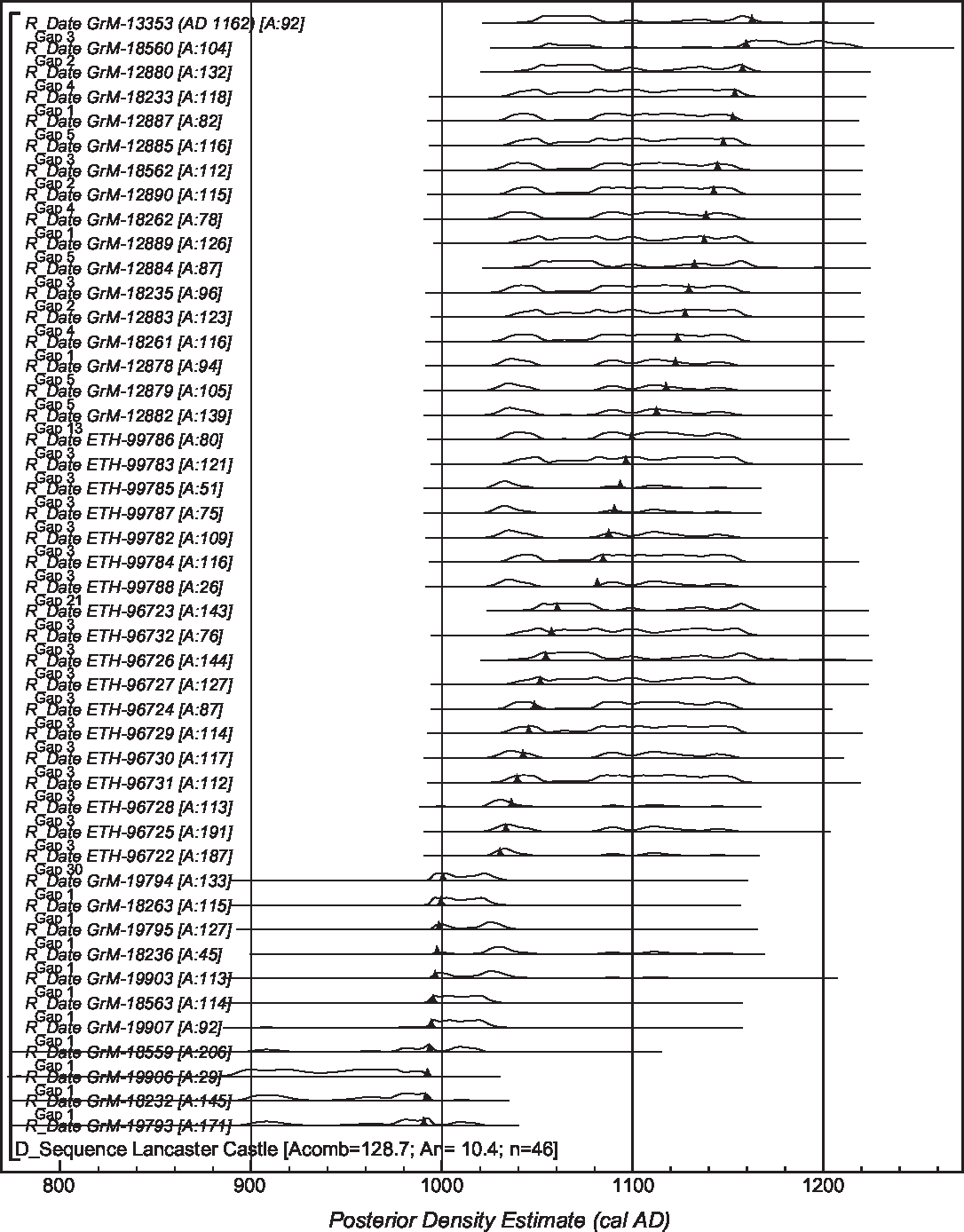
Figure 11 Probability distributions of dates from Lancaster Castle (LAN-C07). Each distribution represents the relative probability that an event occurs at a particular time. For each of the dates two distributions have been plotted: one in outline, which is the result of simple calibration of each 14C measurement independently, and a solid one, based on the wiggle-match sequence. The large square brackets down the left-hand side of the diagram along with the CQL2 keywords (Bronk Ramsey Reference Bronk Ramsey2009) define the model exactly.
Radiocarbon dating of the Lancaster Castle samples was undertaken by the Centre for Isotope Research, University of Groningen (GrM-), the Netherlands in 2018–2019, and at the Laboratory of Ion Beam Physics, ETH Zürich (ETH-), Switzerland in 2019. In Groningen, each ring was converted to α-cellulose using an intensified aqueous pretreatment (Dee et al. Reference Dee, Palstra, Aerts-Bijma, Bleeker, de Bruijn, Ghebru, Jansen, Kuitems, Paul, Richie, Spriensma, Scifo, van Zonneveld, Verstappen-Dumoulin, Wietzes-Land and Meijer2020) and combusted in an elemental analyzer (IsotopeCube NCS), coupled to an isotope ratio mass spectrometer (Isoprime 100). The resultant CO2 was graphitized by hydrogen reduction in the presence of an iron catalyst (Wijma et al. Reference Wijma, Aerts, van der Plicht and Zondervan1996; Aerts-Bijma et al. Reference Aerts-Bijma, Meijer and van der Plicht1997). The graphite was then pressed into aluminium cathodes and dated by AMS (Synal et al. Reference Synal, Stocker and Suter2007; Salehpour et al. Reference Salehpour, Håkansson, Possnert, Wacker and Synal2016). In Zürich, cellulose was extracted from each ring using the base-acid-base-acid-bleaching (BABAB) method described by Němec et al. (Reference Němec, Wacker, Hajdas and Gäggeler2010a), combusted and graphitized as outlined in Wacker et al. (Reference Wacker, Němec and Bourquin2010a), and dated by AMS (Synal et al. Reference Synal, Stocker and Suter2007; Wacker et al. Reference Wacker, Bonani, Friedrich, Hajdas, Kromer, Němec, Ruff, Suter, Synal and Vockenhuber2010b). At both laboratories data reduction was undertaken as described by Wacker et al. (Reference Wacker, Christl and Synal2010c), and both facilities maintain continual programs of quality assurance procedures (Sookdeo et al. Reference Sookdeo, Kromer, Büntgen, Friedrich, Friedrich, Helle, Pauly, Nievergelt, Reinig, Treydte, Synal and Wacker2019 in this issue; Aerts-Bijma et al. forthcoming), in addition to participation in international inter-comparison exercises (Wacker et al. Reference Wacker, Scott, Bayliss, Brown, Bard, Bollhalder, Friedrich, Capano, Cherkinsky, Chivall, Culleton, Dee, Friedrich, Hodgins, Hogg, Kennett, Knowles, Kuitems, Lange, Miyake, Nadeau, Nakamura, Naysmith, Olsen, Omori, Petchey, Philippsen, Bronk Ramsey, Prasad, Seiler, Southon, Staff and Tuna2020 in this issue).
The results (Table 4) are conventional radiocarbon ages, corrected for fractionation using δ13C values measured by AMS (Stuiver and Polach Reference Stuiver and Polach1977). Figure 11 shows a wiggle-match that includes the complete series of results from LAN-C07. It suggests that the final ring was formed in cal AD 1161–1164 (95% probability; GrM-13353 (AD 1162); Figure 11Footnote 6). This result is clearly compatible with the date of AD 1162 for this ring known from dendrochronology. It is, however, rare that such a long ring sequence is recovered from a timber of a historic building in England. For this reason, we have divided this sequence into smaller sections that reflect the kinds of tree-ring sequences that are commonly encountered, and remain undated by ring-width dendrochronology, in English standing buildings.
Figure 12(A) shows a wiggle-match that includes 11 measurements on single-year samples (GrM) between AD 990 and AD 1000 (960–950 cal BP), which produces a date estimate for the final ring of this timber of cal AD 1160–1165 (95% probability; AD 1162; Figure 12(A)). This sequence is very short—only 11 years—but targets the rapid increase in 14C production in AD 993/4 (957/956 cal BP; Figure 3; Miyake et al. Reference Miyake, Masuda and Nakamura2013).

Figure 12 Probability distributions of dates from Lancaster Castle (LAN-C07). A) shows samples from AD 990–1000; B) shows samples from AD 1030–1060; C) shows samples from AD 1081–1099; and D) shows samples from AD 1112–1162. The format is identical to that of Figure 11. The large square brackets down the left-hand side of the diagrams along with the CQL2 keywords define the models exactly.
A wiggle-match that includes 11 measurements on single-year samples (ETH) every three years between AD 1030 and AD 1060 (920–890 cal BP) is shown on Figure 12(B). This estimates that the final ring of LAN-C07 formed in cal AD 1156–1167 (91% probability; AD 1162; Figure 12(B)) or cal AD 1237–1242 (4% probability). This sequence is also too short (31 rings) to be routinely datable by dendrochronology, but targets a steeply sloping section of the calibration curve (Figure 3). IntCal20 was compiled before the candidate solar energetic particle event at AD 1052 was identified (Brehm et al. Reference Brehm, Bayliss, Christl, Synal, Adolphi, Beer, Muscheler, Solanki, Usoskin, Bleicher, Bollhalder, Tyers and Submittedsubmitted), and so does not include additional knots in the spline to maximize the identification of this feature (Heaton et al. Reference Heaton, Blaauw, Blackwell, Bronk Ramsey, Reimer and Scott2020 in this isuse).
Figure 12(C) illustrates a wiggle-match that includes seven measurements on single-year samples (ETH) every three years between AD 1081 and AD 1099 (869–851 cal BP). It suggests that the final ring of the timber dates to cal AD 1107–1117 (16% probability; AD 1162; Figure 12(C)) or cal AD 1160–1170 (7% probability) or cal AD 1173–1198 (72% probability). This sequence is also very short (19 years) and falls on a gently sloping section of curve (Figure 3).
Finally, Figure 12(D) illustrates a wiggle-match across a plateau on the calibration curve (Figure 3). This includes 17 measurements on single-year samples (GrM) at intermittent intervals between AD 1112 and AD 1162 (838–788 cal BP), thus spanning 50 calendar years. It suggests that the final ring of LAN-C07 was formed in cal AD 1156–1166 (95% probability; GrM-13353 (AD 1162); Figure 12(D)).
Clearly these four wiggle-matches all produce date estimates that include the calendar date of AD 1162 for the final ring known from dendrochronology. They are of varying length, some extremely short (< 30 rings), and produce results of varying precision. Even on a plateau, however, it appears possible to produce an accurate chronology to a decadal precision if a long enough sequence and sufficient measurements are available. This represents an opportunity for IntCal20 in areas where high-resolution data are available.
We now consider the single-year case studies that have been undertaken previously (Tyers et al. Reference Tyers, Sidell, van der Plicht, Marshall, Cook, Bronk Ramsey and Bayliss2009; Bayliss et al. Reference Bayliss, Marshall, Tyers, Bronk Ramsey, Cook, Freeman and Griffiths2017; Marshall et al. Reference Marshall, Bayliss, Farid, Tyers, Bronk Ramsey, Cook, Doğan, Freeman, İlkmen and Knowles2019)Footnote 7, each of which has been recalculated using IntCal20 (Table 5). The results are very similar to those produced by IntCal13 (Bayliss et al. Reference Bayliss, Marshall, Tyers, Bronk Ramsey, Cook, Freeman and Griffiths2017: table 5; Marshall et al. Reference Marshall, Bayliss, Farid, Tyers, Bronk Ramsey, Cook, Doğan, Freeman, İlkmen and Knowles2019: figs 3–4), with the wiggle-match sequences from timbers BAG-B18, BCB-10, and KLV-A06 producing Highest Posterior Density intervals that do not include the date for the final ring known from dendrochronology at even 99% probability. Clearly, the absence of single-year calibration data for the medieval period was not the cause of this inaccuracy. By calculating the weighted mean offset between the measurements on these known-age timbers and the IntCal20 modeled value for the respective year, it is clear that the sequences that produce inaccurate results have both the largest offsets against IntCal20 and the highest χ2red values (Figure 13). This suggests both that there are systematic biases in some of these data and that the quoted errors on some of these measurements may be too small. Inter-comparison studies clearly demonstrate that issues of this kind should not be unexpected (Scott et al. Reference Scott, Cook, Naysmith and Staff2019; Wacker et al. Reference Wacker, Scott, Bayliss, Brown, Bard, Bollhalder, Friedrich, Capano, Cherkinsky, Chivall, Culleton, Dee, Friedrich, Hodgins, Hogg, Kennett, Knowles, Kuitems, Lange, Miyake, Nadeau, Nakamura, Naysmith, Olsen, Omori, Petchey, Philippsen, Bronk Ramsey, Prasad, Seiler, Southon, Staff and Tuna2020 in this issue) and, as this example demonstrates, can be a threat to the accuracy of chronologies produced using IntCal20. For such studies, laboratory quality assurance protocols are clearly paramount, and laboratory reproducibility of the type illustrated in Wacker et al. (Reference Wacker, Scott, Bayliss, Brown, Bard, Bollhalder, Friedrich, Capano, Cherkinsky, Chivall, Culleton, Dee, Friedrich, Hodgins, Hogg, Kennett, Knowles, Kuitems, Lange, Miyake, Nadeau, Nakamura, Naysmith, Olsen, Omori, Petchey, Philippsen, Bronk Ramsey, Prasad, Seiler, Southon, Staff and Tuna2020 in this issue: figure 2 [green]) is clearly required.
Table 5 Results of wiggle-matching radiocarbon results from known-age timbers from historic buildings in England using IntCal20 (intervals in bold do not include the age known from dendrochronology).
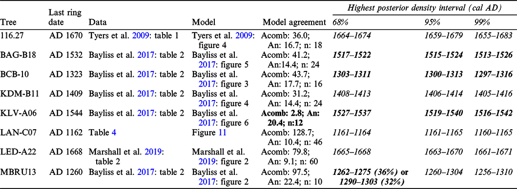

Figure 13 Offsets, indicating model fit, between radiocarbon measurements on single-ring samples from known-age timbers from England (Table 5) and the interpolated value of IntCal20 for the same calendar year, error bars at 1σ (weighted mean difference; Bevington and Robertson Reference Bevington and Robinson1992: equation 4.19: reduced chi-square statistic; Bevington Reference Bevington and Bevington1969: 69).
This case study demonstrates both the opportunities and the threats of using IntCal20 in periods where high-resolution single-year calibration data are now available. It is possible to obtain routinely decadal precision when wiggle-matching timbers from historic buildings, and it is possible to wiggle-match accurately to this precision with shorter ring sequences than can usually be dated by dendrochronology. The accuracy of the measurements that are calibrated or modeled against IntCal20 is, however, a material factor in whether the chronologies produced are correct. Given that the overdispersion of the IntCal20 tree-ring data, even including the factors additional to inter-laboratory variation included in this estimate described above, is one fifth of that for tree-ring measurements reported in the international inter-laboratory comparison exercises (Scott et al. Reference Scott, Naysmith and Cook2018; Heaton et al. Reference Heaton, Blaauw, Blackwell, Bronk Ramsey, Reimer and Scott2020 in this issue: figure 5), most laboratories are clearly not producing measurements of equivalent accuracy to those included in the calibration datasets.
Neolithic Long Barrows in Central-Southern Britain
We now consider the IntCal20 tree-ring data in a specific part of the 4th millennium cal BC, 3690–3635 cal BC (5639–5584 cal BP), relevant to the chronological modeling of a series of Neolithic long barrows in central-southern England (Bayliss and Whittle Reference Bayliss and Whittle2007). In this period IntCal20 includes measurements from four laboratories: decadal data from Seattle (QL-, 1-14), bi-decadal from Belfast (UB, 2-3), single-year data from Groningen (GrN, 4-1), and new 2-year data from ETH, Zürich (ETH, 69-46) (Figure 14). All these measurements were undertaken on European oaks from the Hohenheim or Belfast long chronologies and range in latitude from 55.1°N to 48.4°N.

Figure 14 Radiocarbon results on known-age tree rings 3900–3500 BC (5849–5449 cal BP) (QL, 1-14; UB, 2-3; GrN, 4-1; ETH, 69-49); A) with IntCal04 and IntCal20, B) and GrN/ETH only and QL/UB only curves created for this sensitivity analysis using the IntCal20 methodology (error bars and envelopes at 1σ).
The new dataset is derived from a sub-fossil oak tree (sample 60) from Ebensfeld, River Main, Germany (50.1N, 10.9E). The 92-year ring-width series cross-dates with a t-value of 5.5 (Baillie and Pilcher Reference Baillie and Pilcher1973) to the Holocene German Oak Chronology (Friedrich et al. Reference Friedrich, Remmele, Kromer, Hofmann, Spurk, Felix Kaiser, Orcel and Küppers2004), when it spans 3691–3600 BC (5640–5549 cal BP; Supplementary Information 1). Dissection was undertaken by Michael Friedrich, on radial sections cut from the slices taken for dendrochronology. The rings had been made visible by cleaning their surfaces using razor blades, the selected blocks were split tangentially from the rest of the sample using a scalpel blade. Each sample consisted of two annual growth rings, including both early and latewood.
A base-acid-base-acid-bleaching was applied for cleaning and cellulose extraction (Němec et al. Reference Němec, Wacker, Hajdas and Gäggeler2010a). Kauri wood (ETH-44660) and brown coal (ETH-38779) from Reichewalde, Germany, significantly older than 60 kyr served as reference processing blanks, and a dendrochronologically dated ring (AD 1515; ETH-40759; Brehm et al. Reference Brehm, Bayliss, Christl, Synal, Adolphi, Beer, Muscheler, Solanki, Usoskin, Bleicher, Bollhalder, Tyers and Submittedsubmitted: figure S5.1) of a Swiss pine was used as a secondary standard (Güttler et al. Reference Güttler, Wacker, Kromer, Friedrich and Synal2013). The blanks and secondary standards were prepared in parallel with the calibration samples applying the same cleaning steps. All samples, and the unprocessed OX-II standards, were graphitized on the fully automated graphitization equipment (AGE) system (Němec et al. Reference Němec, Wacker and Gäggeler2010b; Wacker et al. Reference Wacker, Němec and Bourquin2010a). Samples were analyzed in the MICADAS system (Wacker et al. Reference Wacker, Bonani, Friedrich, Hajdas, Kromer, Němec, Ruff, Suter, Synal and Vockenhuber2010b). In addition to the wood samples, each cassette contained two processed blanks and seven OX-II standards for normalization. Data analysis and evaluation was performed using the computer programme BATS (Wacker et al. Reference Wacker, Christl and Synal2010c). The uncertainties in 14C age are derived from counting statistics, standards normalization, and sample preparation. The 14C counts were background corrected using the processed blank and normalized with OX-II standards. Additional uncertainty (1‰ in Δ14C, or equivalently 8 BP in radiocarbon age), estimated from long-term laboratory statistics on processed secondary wood standards, was added in quadrature. The measured 14C concentrations for the Ebensfeld tree rings are given in Supplementary Information 2.
The four datasets that cover the 37th century BC (5648–5549 cal BP) clearly show divergence across some of this period (Figure 14). The ETH and GrN data are generally closer to each other than they are to the QL and UB data (which closely follow each other). This is particularly apparent in the 3660s BC (5610s cal BP) when both the ETH and GrN datasets appear to suggest a much larger wiggle than is apparent in the QL/UB data. Given the much higher density of the ETH dataset, IntCal20 follows it closely, whereas previous versions of the calibration curve struck a more balanced path between the higher density, but lower resolution, QL and UB datasets and the high-resolution, but sparse, GrN data (Figure 14A). Given the small range in latitude of the dated trees (less than seven degrees) and what we know of the expected scale of locational and inter-tree variation, this offset appears to originate from either sub-decadal variations in atmospheric radiocarbon, or from inter-laboratory differences, or from a combination of these. Pending further high-resolution datasets for this period, IntCal20 represents the best estimate of the radiocarbon calibration curve for these decades. There is clearly disagreement between the underlying data, however, which is only apparent because we have multiple datasets, some of which are at high resolution. The ETH dataset in this period (69-46) constitutes 69 of the 303 new measurements in IntCal20 in the 8000 years between 4000 and 12000 cal BP (2051–10,051 BC). For most periods of prehistory we simply do not have data of this kind, and so further issues of this type are clearly not only possible within this timespan, but should be expected.
Such unrecognised refinements in the concentration of atmospheric radiocarbon are a potential threat of which users of IntCal20 must be aware when comparing radiocarbon-based chronologies with historical or dendrochronological timescales. As a sensitivity analysis, to explore the effects such future refinements may have on archaeological interpretation, we have constructed two, alternative calibration curves for this period using the IntCal20 methodology (Heaton et al. Reference Heaton, Blaauw, Blackwell, Bronk Ramsey, Reimer and Scott2020 in this issue): one only including datasets 4-1 and 69-46 (GrN/ETH) and the other only including datasets 1-14 and 2-3 (QL/UB) (Figure 14B). Figure 15 shows differences between the calibrated date ranges provided for a measurement of 4910 BP, with errors of ± 70 BP, ± 35 BP, and ± 15 BP, when this is calibrated using IntCal04, IntCal20, and the two variant calibration curves constructed for this sensitivity analysis. The medians for the four calibrations in each group vary by a maximum of seven calendar years. Clearly this is not a substantive concern for archaeological interpretation.

Figure 15 Radiocarbon results of 4910 ± 70 BP, 4910 ± 35 BP, and 4910 ± 15 BP, calibrated using the probability method (Stuiver and Reimer Reference Stuiver and Reimer1993) and IntCal20 (black), IntCal04 (red), GrN/ETH only (orange), and QL/UB only (blue).
The original analysis of the five long barrows (Bayliss and Whittle Reference Bayliss and Whittle2007) from central-southern England was undertaken using OxCal v3.10 (Bronk Ramsey Reference Bronk Ramsey1995) and IntCal04 (Reimer et al. Reference Reimer, Baillie, Bard, Bayliss, Beck, Bertrand, Blackwell, Buck, Burr, Cutler, Damon, Edwards, Fairbanks, Friedrich, Guilderson, Hogg, Hughen, Kromer, McCormac, Manning, Bronk Ramsey, Reimer, Remmele, Southon, Stuiver, Talamo, Taylor, van der Plicht and Weyhenmeyer2004). We have reprogrammed the preferred models from this study in CQL2 (Bronk Ramsey Reference Bronk Ramsey2009) as discussed in Supplementary Information 3, and recalculated them using using IntCal04, IntCal20, and the two variant calibration curves constructed for this sensitivity analysis. Key parameters calculated using IntCal04 (red) and IntCal20 (black) are shown in Figure 16, and key parameter calculated using the GrN/ETH only curve (orange) and QL/UB only curve (blue) are shown in Figure 17.

Figure 16 Probability distributions of major archaeological events at Ascott-under-Wychwood, Fussell’s Lodge, Hazleton, West Kennet, and Wayland’s Smithy long barrows. The estimates are based on the preferred chronological models illustrated by Bayliss et al. (Reference Bayliss, Benson, Galer, Humphrey, McFadyen and Whittle2007a: figures 3, 5–7); Wysocki et al. (Reference Wysocki, Bayliss and Whittle2007: figures 10–11); Meadows et al. (Reference Meadows, Barclay and Bayliss2007: figures 6–9), Bayliss et al. (Reference Bayliss, Whittle and Wysocki2007b: figure 6) and Whittle et al. (Reference Whittle, Bayliss and Wysocki2007: figure 4) reprogrammed using OxCal 4.3 (Bronk Ramsey Reference Bronk Ramsey2009) as described in Supplementary Information 3 and calculated using IntCal04 (Reimer et al. Reference Reimer, Baillie, Bard, Bayliss, Beck, Bertrand, Blackwell, Buck, Burr, Cutler, Damon, Edwards, Fairbanks, Friedrich, Guilderson, Hogg, Hughen, Kromer, McCormac, Manning, Bronk Ramsey, Reimer, Remmele, Southon, Stuiver, Talamo, Taylor, van der Plicht and Weyhenmeyer2004 [red]) and IntCal20 (Reimer et al. Reference Reimer, Austin, Bard, Bayliss, Blackwell, Bronk Ramsey, Butzin, Cheng, Edwards, Friedrich, Grootes, Guilderson, Hajdas, Heaton, Hogg, Hughen, Kromer, Manning, Muscheler, Palmer, Pearson, van der Plicht, Reimer, Richards, Scott, Southon, Turney, Wacker, Adolphi, Büntgen, Capano, Fahrni, Fogtmann-Schultz, Friedrich, Kudsk, Miyake, Olsen, Reinig, Sakamoto, Sookdeo and Talamo2020 in this issue [black]).

Figure 17 Probability distributions of major archaeological events at Ascott-under-Wychwood, Fussell’s Lodge, Hazleton, West Kennet, and Wayland’s Smithy long barrows. The estimates are based on the preferred chronological models illustrated by Bayliss et al. (Reference Bayliss, Benson, Galer, Humphrey, McFadyen and Whittle2007a: figures 3, 5–7); Wysocki et al. (Reference Wysocki, Bayliss and Whittle2007: figures 10–11); Meadows et al. (Reference Meadows, Barclay and Bayliss2007: figures 6–9), Bayliss et al. (Reference Bayliss, Whittle and Wysocki2007b: figure 6) and Whittle et al. (Reference Whittle, Bayliss and Wysocki2007: figure 4) reprogrammed using OxCal 4.3 (Bronk Ramsey Reference Bronk Ramsey2009) as described in Supplementary Information 3 and calculated using the alternative calibration curves compiled using the IntCal20 methodology (Heaton et al. Reference Heaton, Blaauw, Blackwell, Bronk Ramsey, Reimer and Scott2020 in this issue) for this sensitivity analysis, GrN/ETH data only (orange), QL/UB data only (blue).
For parameters dating to the end of the 37th and 36th centuries cal BC, differences are very slight (medians vary by an average of 5 years and a maximum of 14). The important archaeological findings from the long barrows study—that the primary phase of burial in four of the tombs ended within a decade or two of 3625 cal BC, and that the initial construction of Wayland’s Smithy belongs to the following human generation—appear robust. The posterior distributions of parameters that fall in the late 38th century and early and mid-37th century cal BC are more variable, however (medians vary by an average of 22 years and a maximum of 39). The potential for the initial construction dates of Fussell’s Lodge and Ascott-under-Wychwood all to be a generation or so later has two implications. First, these constructions may belong to an even more concentrated horizon, spanning hardly more than a single human lifetime, in the middle part of the 37th century cal BC. Second, the variation in the duration of the initial period of burial in these monuments is also reduced, so that none need to have been in use for more than two or three generations. At all these sites, burial may not have outlasted the living memory of those in the community who witnessed their construction. This would have important implications for our understanding of Neolithic society.
This case study illustrates the strengths and weaknesses of IntCal20 in the period where there is little new data (i.e. in the 8000 years between 4000 and 12,000 cal BP). Decadal and bi-decadal calibration data are sufficient for calibrating single radiocarbon dates accurately (indeed, this is the purpose for which these data were originally obtained). Higher resolution data will uncover sub-decadal changes in the level of atmospheric radiocarbon that are invisible from the existing data. In this example, we see that changes in posterior distributions from chronological models range from less than a decade to a few decades. A few decades is a long time in a narrative at the scale of lifetimes and generations, and can have important implications for archaeological interpretation. But these differences are no more than those observed from modeling different archaeological interpretations of the sequence at these sites in the original studies (e.g. Wysocki et al. Reference Wysocki, Bayliss and Whittle2007: figure 12).
CONCLUSIONS
For the previous generation of research, the part of the radiocarbon calibration curve based on tree rings has been seen as something of a “gold standard” to which other archives can but aspire. More than 90% of the tree-ring data in IntCal20 that was inherited from IntCal13, however, was measured in the 1980s or 1990s. In the intervening two decades, while there has been some extension at the earlier part of the tree-ring dataset (e.g. Kromer et al. Reference Kromer, Friedrich, Hughen, Kaiser, Remmele, Schaub and Talamo2004) and some replication in periods of particular interest (e.g. Kromer et al. Reference Kromer, Manning, Friedrich, Talamo and Trano2010), the major advance in radiocarbon calibration has been the provision of a calibration curve to the limit of the technique based on a variety of other archives (Reimer et al. Reference Reimer, Bard, Bayliss, Beck, Blackwell, Bronk Ramsey, Buck, Cheng, Edwards, Friedrich, Grootes, Guilderson, Haflidason, Hajdas, Hatté, Heaton, Hoffmann, Hogg, Hughen, Kaiser, Kromer, Manning, Niu, Reimer, Richards, Scott, Southon, Staff, Turney and van der Plicht2013).
IntCal20 clearly reflects recent technological advances in AMS that enable high-precision measurements to be made in large numbers on single tree rings (Wacker et al. Reference Wacker, Bonani, Friedrich, Hajdas, Kromer, Němec, Ruff, Suter, Synal and Vockenhuber2010b, Reference Wacker, Scott, Bayliss, Brown, Bard, Bollhalder, Friedrich, Capano, Cherkinsky, Chivall, Culleton, Dee, Friedrich, Hodgins, Hogg, Kennett, Knowles, Kuitems, Lange, Miyake, Nadeau, Nakamura, Naysmith, Olsen, Omori, Petchey, Philippsen, Bronk Ramsey, Prasad, Seiler, Southon, Staff and Tuna2020 in this issue). This has fostered a renewed interest in obtaining an annual record of atmospheric radiocarbon in the past and for understanding its locational and other variations. Ultimately this will have important implications for the accuracy and precision of archaeological chronologies, particularly those that are based on the formal statistical modeling of suites of radiocarbon dates. At present, however, the part of the calibration curve based on tree rings varies in resolution and replication through time, with single-year data concentrated in five of the fourteen millennia covered by the tree rings, and rarely replicated outside the most recent millennium. The part of IntCal20 that is based on tree rings thus represents a transition: from a calibration curve largely based on decadal and bi-decadal blocks of tree rings, to one based on higher resolution datasets. Opportunities for increased precision and accuracy using IntCal20 are thus currently variable, and anyway do not come without risks, as accurate chronologies will only be produced if the radiocarbon measurements on the archaeological samples that are calibrated against the curve are of equivalent accuracy.
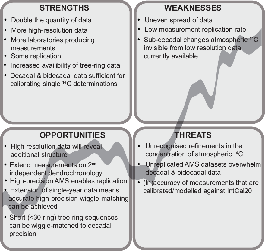
Radiocarbon calibration is a work in progress. IntCal20 has strengths and weaknesses (Figure 18). It contains more than double the quantity of data than IntCal13, and that data is of higher resolution and has been produced by a larger number of laboratories. There is also much more replication than before, although this is still on a relatively limited scale. High-resolution data are currently only available for part of the tree-ring timescale, and so for the majority of its extent there may be sub-decadal changes in atmospheric radiocarbon that are invisible from the data that are currently available. These sub-decadal changes provide an opportunity for archaeologists to produce more robust chronologies for the past, as not only the accuracy of radiocarbon calibration improves but as the precision of, particularly, modeled date estimates increases. Higher resolution data may reveal structure in what are currently intractable plateaux, and more detailed understanding of the shape of the calibration curve may be exploited to provide precise chronologies for shorter sequences. These opportunities come with threats. They make stringent demands of the accuracy not only of the, often unreplicated, high-resolution calibration data but also of the measurements that are obtained by archaeologists on their samples. If these are lacking, chronologies that are not accurate within their quoted uncertainties may be produced. Clearly there is a threat that not all the sub-decadal changes in past atmospheric radiocarbon are visible in IntCal20, and that there may be more locational variation than is currently apparent. IntCal20 does, however, combine the extensive amount of calibration data that is now available using an explicit statistical methodology to account for the observed variability and provides a common standard calibration for use by archaeologists.

Figure 18 IntCal20 tree rings SWOT analysis matrix.
We would like to end on a positive note, by considering how our SWOT analysis may be used to inform a strategy for future enhancements of radiocarbon calibration: building on the strengths identified, tackling the weaknesses, exploiting the opportunities, and mitigating the threats. There is much research required to maximize the utility of radiocarbon dating in archaeology and safeguard its reputation in the discipline, including the following (by no means exhaustive list):
secure the accuracy of datasets included in IntCal through greater measurement replication, including both repeat measurements on the same sample by a single laboratory, and repeat measurements on that sample by two or more laboratories;
extend and replicate single-year measurements through the Holocene so that additional structure in high resolution data can be exploited for archaeological/palaeoenvironmental/climatic reconstructions, etc;
address the uneven spread of measurements across the potential extent of tree-ring-based calibration through a more coordinated approach;
investigate potential additional sources of variation due to intra-hemispheric locational, latitudinal, and species differences (the availability of multiple independent dendrochronologies around the hemisphere in the last few thousand years presents a particular opportunity);
ensure the accuracy of measurements that are calibrated or modeled against future iterations of IntCal through on-going inter-comparison exercises, and the use of a common suite of laboratory standards.
Clearly, the need of archaeological users for more accurate calibration is only one, and not necessarily the principal, driver for research into the past levels of atmospheric radiocarbon. But the archaeological perspective can strengthen studies, even where their primary focus is elsewhere. As the IntCal initiative itself so powerfully demonstrates, the research community is stronger when working together across disciplinary boundaries.
ACKNOWLEDGMENTS
We would like to thank Bisserka Gaydarska for her help in collating the Northern Hemisphere tree-ring and radiocarbon data for IntCal20, and Alison Arnold and Robert Howard (Nottingham Tree-ring Dating Laboratory) who undertook the dissection of the core from Lancaster Castle. Bisserka Gaydarska, Frances Healy, Jonathan Palmer, Alasdair Whittle, and two anonymous referees kindly provided feedback on the draft of this paper. TJ Heaton is supported by a Leverhulme Trust Fellowship (RF-2019-140\9). We are also grateful to Paula Reimer and Alan Hogg for their support and encouragement.
Supplementary material
To view supplementary material for this article, please visit https://doi.org/10.1017/RDC.2020.77


 Open access