


INTRODUCTION
Radiocarbon (14C) dating is used in a wide range of research disciplines, including archaeology, geology, paleobotany, sedimentology, karst studies and paleoclimatology. The number of samples processed for 14C dating is still increasing every year. Obviously, users request as high precision as possible. Better time resolution can help to resolve some unanswered research issues, which can sometimes be resolved with this increased resolution.
The most precise dating results use the dendrochronological method for the dating of wooden artifacts. This method is limited by minimum number of tree rings (Prokop et al. Reference Prokop, Kolář, Kyncl and Rybníček2017). It is suggested that tree-ring width series should not be shorter than 40 (Cook and Kairiūkštis Reference Cook and Kairiūkštis1990) or even 50 years (Haneca et al. Reference Haneca, Čufar and Beeckman2009; Rybníček et al. Reference Rybníček, Čermák, Žid, Kolář, Trnka and Büntgen2015, Reference Rybníček, Chlup, Kalábek, Kalábková, Kočár, Kyncl, Muigg, Tegel, Vostrovská and Kolář2018) for precise dating. In addition, wood species identification, provenance of samples and existence of a tree-ring width chronology are essential inputs for successful dendrochronological dating. Also, excellent time resolution can be reached by using the radiocarbon wiggle-matching method and such results can approach dendrochronological precision, if sufficiently long sequences of tree rings are available (van der Plicht and Mook Reference van der Plicht and Mook1989; Bleicher Reference Bleicher2014; Jacobsson et al. Reference Jacobsson, Hale, Cook and Hamilton2018; Krapiec et al. Reference Krapiec, Michczynska, Michczynski, Piotrowska, Goslar and Szychowska-Krapiec2018; McDonald et al. Reference McDonald, Chivall, Miles and Ramsey2018). Unfortunately, the majority of samples for radiocarbon dating (archaeological, geological, etc.) are isolated samples, without the possibility of grouping them with other samples with a known relative time gap.
Using high-precision accelerator mass spectrometry (AMS) measurements, we can determine 14C activity with uncertainties of about 15 years of conventional radiocarbon age in samples several thousand years old. The current internationally agreed calibration curves for dating of the terrestrial samples are IntCal13 for the Northern Hemisphere (Reimer et al. Reference Reimer, Bard, Bayliss, Beck, Blackwell, Ramsey, Buck, Cheng, Edwards, Friedrich, Grootes, Guilderson, Haflidason, Hajdas, Hatté, Heaton, Hoffmann, Hogg, Hughen, Kaiser, Kromer, Manning, Niu, Reimer, Richards, Scott, Southon, Staff, Turney and van der Plicht2013) and SHCal13 for the Southern Hemisphere (Hogg et al. Reference Hogg, Hua, Blackwell, Niu, Buck, Guilderson, Heaton, Palmer, Reimer, Reimer, Turney and Zimmerman2013). For both hemispheres, these curves cover the past 50,000 years.
Over a time scale of several decades, parts of the radiocarbon calibration curves (reported in the years of conventional radiocarbon age) can be differentiated into four main types: (a) relatively monotonic parts of the curve, resulting in one main time interval; (b) fluctuating parts of the curve, with several resulting separate time intervals with similar probabilities, e.g. 1640–1950 AD, which is rather difficult for radiocarbon dating; (c) plateaus in the curve where refining of a radiocarbon measurement uncertainty is not reflected in a narrower time interval, thus, corresponding approximately to a width of the plateau; and (d) relatively steep parts of the curve which enable definite and very narrow time intervals. These various results are shown as examples in Figure 1.
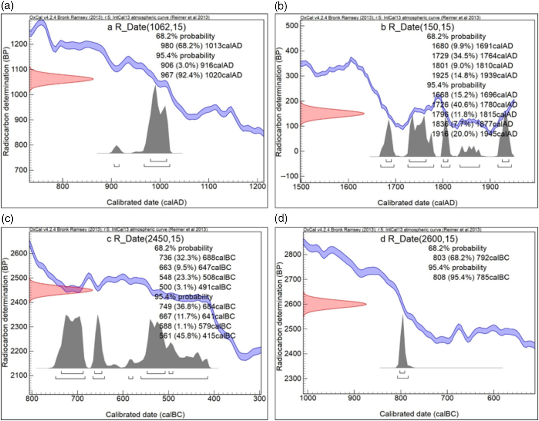
Figure 1 (a)–(d): Examples of characteristic parts of the calibration curve IntCal13 (for better visual comparison is the horizontal scale, about 500 years for each diagram).
The steep parts are often seen close to the edges of a plateau. Thus, under favorable circumstances for 14C dating, it is possible to reach a very narrow resulting time interval. The steep parts of the curve could then be possibly used as a “time magnifier” or an exact “time marker”. Time periods which correspond to the steep parts of the curve have relatively short duration. Therefore, the likelihood of results which would also correspond to these time periods on the steep parts of the curve can be also low. Likewise, dating using steep parts of the calibration curve could be connected with some discrepancies implying small (but significant) differences in 14C activity in the calibration curve and in real samples. This could be caused by slight geographical differences of 14C activity course, by different periods of a wood mass growth caused by small microclimatic differences in examined sites, or by a species of the tree with a different period of wood growth (we can assume that small annual seasonal changes of 14C activity occurred also in the distant past). These regional effects should be amplified in steep section of the curve.
For 14C laboratories and the users of 14C dating, it is very important to provide realistic results with the time intervals which are as precise as reasonably possible. On the other hand, the results should not offer an uncritically high, yet distorted time resolution, which is more likely a result of random influences caused by improper sample selection, insufficient sample treatment or underestimation of related uncertainties, e.g. systematic ones.
The purpose of this study is to provide a basic survey of the time resolution available for radiocarbon dating and validate application of the steep parts of the calibration curve IntCal13 for the purpose of precise radiocarbon dating of solitary samples. It can be assumed that the slope parts of calibration curves can provide a possibility to validate actual curves and their uncertainties. We also recommend some relevant types of samples, which can be proper for precise dating. Relevant samples with known origin from the periods corresponding to the rapid slope sections of the calibration curve can also provide a particularly sensitive “natural” material (due to rapid changes of 14C activity at this period) for testing and comparing sample treatment routines, which are focused on the removal of interfering carbon chemical forms.
METHODS
Following the considerations discussed above, we carried out the first step of the experiment using tree-ring samples. Together with dendrochronologists, we evaluated the 14C activity in tree rings corresponding to the selected steep parts of the actual calibration curve IntCal13.
a) Processing of the IntCal13 curve
The expected resolution of 14C dating of a sample corresponding to a specific calendar age was calculated as the weighted average length of all dating intervals at 95% probability level which contain this date after calibration using the IntCal13 curve. The dating intervals were weighed by the probability distribution of the 14C date after calibration,
 $$ ({r_x} = {{\mathop \sum \nolimits_{i = 1}^n {r_i}{p_{xi}}} \over {\mathop \sum \nolimits_{i = 1}^n {p_{xi}}}}) $$
where r x is the weighted average dating interval length (resolution) at a specific calibrated age x, r i is the length of the interval obtained by calibrating 14C date i (at 95% probability level), p xi is the value from the probability distribution of the date i after calibration at calendar age.x Since we used the uncalibrated 14C dates from the IntCal13 dataset as input data, n is the number of records in this dataset. To obtain probability distributions in calendar years for each date, we calibrated them using the same IntCal13 curve while assuming an uncertainty of measurement proportional to their radiocarbon age.
We assumed that the uncertainty of 14C analyses of samples with activity (reported as Conventional Radiocarbon Age) about 0 BP is just 15 yr BP (Stuiver and Polach Reference Stuiver and Polach1977). Uncertainties of the samples with lower activities were calculated using the formula:
 $$ ({u_i} = {u_1}.{e^{{{ + {A_i}} \over {2.8033}}}}) $$
where u i is the expected uncertainty of 14C analysis of the sample at a specific radiocarbon age, i u 1 is the expected uncertainty of analysis of 15 yr BP (for a sample with activity 0 yr BP), A i is the activity (reported as 14C yr BP) of the sample.
b) Selection of relevant tree rings
All samples were taken from archaeological or subfossil findings from the eastern part of the Czech Republic, as shown in Table 1. After careful surface preparation to maximize the visibility of tree-ring borders (Gärtner and Nievergelt Reference Gärtner and Nievergelt2010), tree-ring widths were measured with the VIAS TimeTable system with accuracy of 0.01 mm. The resulting annual ring width values were visually synchronized and cross-dated using PAST4 (Knibbe Reference Knibbe2004), as well as statistically controlled via COFECHA (Grissino-Mayer Reference Grissino-Mayer2001). The final tree-ring width series were dated according to the latest version of the Czech oak tree-ring width chronology (Kolář et al. Reference Kolář, Kyncl and Rybníček2012; Prokop et al. Reference Prokop, Kolář, Kyncl and Rybníček2017; Dobrovolný et al. Reference Dobrovolný, Rybníček, Kolář, Brázdil, Trnka and Büntgen2018). Then, each precisely dated annual oak increment was separated and finely cut (separately for early wood and late wood) with a scalpel or razor blade under a stereomicroscope into small pieces.
c) Description of a sample treatment (at CRL Lab, Prague, Czech Republic) and AMS measurements (at ICER Atomki Lab, Debrecen, Hungary)
Table 1 A list of utilized sequences of oak tree-rings.
The samples were washed repeatedly with 4% HCl followed by 4% NaOH and finally 4% HCl again. Before and after the alkaline extraction, the samples were rinsed with distilled water in order to adjust the pH of the extract to 6–8 (Gupta and Polach Reference Gupta and Polach1985). Subsequently, the samples were dried at 60°C to reach constant weight. After the pretreatment, the dry samples together with a small amount of CuO were torch sealed under a dynamic vacuum into a quartz glass tubes and combusted at 900°C for at least 8 hr. The resulting carbon dioxide was then purified and transferred into the graphitization reactor. The batch method of graphitization with pure Zn as a sole reduction agent was derived from similar routines described by Rinyu et al. (Reference Rinyu, Orsovszki, Futó, Veres and Molnár2015) and by Orsovszki and Rinyu (Reference Orsovszki and Rinyu2015). Following the graphitization step, the samples were sealed in vacuum and sent for AMS measurements to the ICER laboratory in Debrecen with international code “DeA-“ (Molnár et al. Reference Molnár, Janovics, Major, Orsovszki, Gönczi, Veres, Leonard, Castle, Lange, Wacker, Hajdas and Jull2013a, Reference Molnár, Rinyu, Veres, Seiler, Wacker and Synal2013b; Handlos et al. Reference Handlos, Svetlik, Horáčková, Fejgl, Kotik, Brychova, Megisova and Marecova2018).
The measurements were carried out using the EnvironMICADAS compact tandem accelerator (Kromer et al. Reference Kromer, Lindauer, Synal and Wacker2013; Molnár et al. Reference Molnár, Rinyu, Veres, Seiler, Wacker and Synal2013b). Graphitized samples of oxalic acid NIST HOX II SRM 4990-C were used for calibration (Schneider et al. Reference Schneider, McNihol, Nadeau and Reden1995). Graphitized samples of anthracite (preheated under dynamic vacuum at 800°C for at least 15 min) were used for correction of background contributions. The resulting 14C activity and its combined uncertainty are given in yr BP (Before Present) as the conventional radiocarbon age according to Stuiver and Polach (Reference Stuiver and Polach1977), including δ13C correction measured by the MICADAS (Curie 1955).
The calibration software OxCal was used for determination of the sample age; with respect to the available data, the radiocarbon calibration curve IntCal13 was chosen (Bronk and Lee Reference Bronk and Lee2013; Reimer et al. Reference Reimer, Bard, Bayliss, Beck, Blackwell, Ramsey, Buck, Cheng, Edwards, Friedrich, Grootes, Guilderson, Haflidason, Hajdas, Hatté, Heaton, Hoffmann, Hogg, Hughen, Kaiser, Kromer, Manning, Niu, Reimer, Richards, Scott, Southon, Staff, Turney and van der Plicht2013). After assignment of uncertainties given by the radiocarbon calibration curve, the conventional radiocarbon age and its combined uncertainty were converted to calibrated age intervals (Table 3).
Table 3 Results of 14C analyses of tree rings dated by dendrochronology.
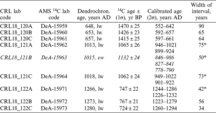
* The main interval.
RESULTS
Using the routine described above, we obtained a diagram of the dependence of the possible time resolution for a sample calibrated age (Figure 2).
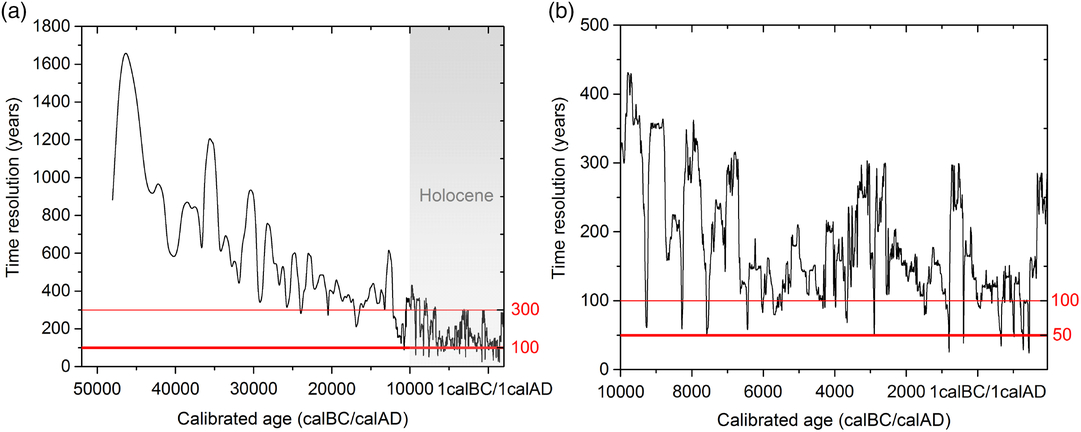
Figure 2 Dependence of the time resolution of the radiocarbon dating method (for 2σ interval of 14C analyses) on the calibrated age of the sample (reported in the years calBC/calADFootnote 1 ); two or more resulting time intervals are integrated into one “covering” interval (the absolute probability of such integrated intervals is slightly exceeding the declared 95% for two sigma): (a) The whole scale covered by IntCal13 with highlighted time resolutions of 100 years (bold red line) and 300 years (thin red line); (b) Holocene epoch in detail with highlighted time resolutions of 50 years (bold red line) and 100 years (thin red line). (Please see electronic version for color figures.).
The intervals of the improved time resolution found for Holocene samples using IntCal13 (for time interval widths below 50 years of the calibrated age) are reported in Table 2, including minimal width for given interval of the sample origin.
Table 2 Time intervals with the time resolution below 50 years and the minimal possible width in a given interval.
Several samples of tree rings, late wood (lw) from the given year, excluding early wood sample 18_121B (ew), dated by dendrochronology were analyzed with uncertainties above 20 years. A summary of the results obtained is reported in Table 3.
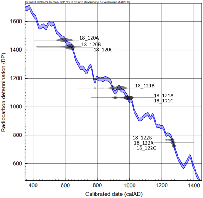
A relation between the results of radiocarbon dating and the year of sample origin, as determined by dendrochronology is shown in Figure 3. As evident from the diagram, there is a visible systematical shift of radiocarbon results toward older periods for both sample sequences 18_120 and 18_121. We have also shown all the results of the radiocarbon dating visualized on the calibration curve in Figure 4.
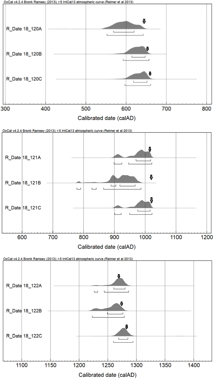
Figure 3 Comparison of radiocarbon dating results (probability density curves) of tree rings with dendrochronology determination (bold arrow) of the year of a given sample origin.

Figure 4 Visualization of the radiocarbon dating results on steep parts of the calibration curve.
DISCUSSION
Using radiocarbon calibration curve IntCal13, six intervals providing time resolution of the sample origin below 50 years were found, with an uncertainty in 14C analyses of ±15 years (14C years) and two sigma interval (±15 years corresponding to analyses of recent samples) for the period covering the last three thousand years (see Table 2). In the case of older periods, 13 time intervals enabling higher time resolution (below 100 years) during the rest of the Holocene (Figure 2a) and 4 intervals below 300 years from 10 ka BC to 24 ka BC (including a wide interval from 10,473 to 12,175 BC) with a subinterval 10,744 to 10,775 BC with possible resolution below 100 years (Figure 2b) were found. On the residual part of IntCal13 calibration curve, we found two local minima with the best time resolution of <400 years.
Using nine dendrochronologically dated tree-ring samples, with uncertainties of 14C analyses using AMS in the range 21–26 yr BP, we obtained eight results which are in agreement with dendrochronology determination (although the resulting time interval of the sample 18_120A is three years below the year found by dendrochronology). All these samples in good agreement were prepared from late wood of the investigated tree rings. In the case of the sample prepared from early wood, a significant difference exceeding 29 years between dendrochronology and “older” radiocarbon dating was found. Despite the fact that uncertainties of 14C analyses substantially exceeded 15 yr BP, the narrowest resulting time interval was 34 years for the sample 18_122C, compared to 29 years obtained for the best possible resolution for this time period.
As evident from Figure 3, there is a visible systematical shift of the radiocarbon dating resulting intervals compared to dendrochronology results. This shift is caused by the systematically smaller 14C activities of the samples analyzed (although on the border of the statistical significance). Such a shift can be probably given by the reduced routine of samples pretreatment, where only acid-alkali-acid leaching was used, without extraction of tree resins and bleaching routines. The reduced routine was applied due to limited amounts of material. Previously, it was shown that for most wood samples the results obtained with this simple method are comparable with more complicated treatments, which have the disadvantage of low yields (Hajdas et al. Reference Hajdas, Hendriks, Fontana and Monegato2017). In the case of neighboring periods, when available time resolution is several times worse, systematical shifts of the resulting time interval will be several times smaller. Likewise, such cases can be judged against the possibility of pretreated sample contamination from the applied reagents, glassware or from laboratory surroundings, which increases with the number of sample preparation steps. In the case of the expected sample origin in the period with a possible fine time resolution, several different routines of the sample pretreatment should be carried out to get comparable results. If there are no significant differences between the results, all these routines can be sufficient for a given sample type, both most “robust” and most “vulnerable”. In the opposite case, several different more “robust” routines should be compared, if the sample quantity would be sufficient. Samples with the origin from “fine time resolution period” seem to be the most sensitive for the comparison of the sample processing routines.
Early wood in oaks at the Czech Republic territory grow from April until the beginning of June. The late wood starts about the first half of June and is usually finished in August. During a cold period of a given year (including spring), decreasing activities of the atmospheric 14CO2 have been observed since the beginning of monitoring of this parameter in the 20th century (Levin et al. Reference Levin, Graul and Trivett1995; Levin and Kromer Reference Levin and Kromer1997, Reference Levin and Kromer2004). It can be presumed that annual seasonal changes of 14CO2 activity occurred also in the past (McDonald et al. Reference McDonald, Chivall, Miles and Ramsey2018). The second influence, causing decreased 14C activities of early wood can be connected with elevated amount of allochthonous carbon forms (especially humic and fulvic acids) due to the increased porosity of such samples (Vavrčík et al. Reference Vavrčík, Gryc and Rybníček2008; Shchupakivskyy et al. Reference Shchupakivskyy, Clauder, Linke and Pfriem2014). Hence, in this case it would be interesting to carry out a sample pretreatment using extended routines (bleaching and extraction of resins). Nevertheless, to obtain more conclusive data, a greater collection of early wood samples from this period would be needed.
In general, for the purpose of accurate radiocarbon dating, samples with a well-defined and short period of sample formation can be used, e.g. late wood from tree rings, fine tree branches (representing only several years of growth), plant seeds, plant macrofossils, animal/human teeth, fatty acids, or fine sediment layers with distinctive summer/winter lamination.
In contrast, there are samples with a longer period of growth (several decades) and with unclear speed of sample formation/accumulation such as charcoal powder, bone collagen, pollen concentrates, carbon from historical steel, peat and karst sinters. In this case, the uncertainty of 14C analyses should be expanded in the relation with the estimated period of the sample formation. Results of radiocarbon dating then should be reported as intervals corresponding to time mean of the sample formation, supposing processed and measured sample fraction to be homogenous.
When a sufficient sequence of (tree-ring) samples with known time gap is available, the wiggle-matching method (WM) provides results with a time resolution of several years for the Holocene period (Hogg et al. Reference Hogg, Gumbley, Boswijk, Petchey, Southon, Anderson, Roa and Donaldson2017). Although the dendrochronology dating results in an even better time resolution of a single year, the wiggle-matching method provides absolute dating independently of local calibration scales (in the general). Demands on quality of wood material are relatively low in the case of WM method, but compared to dendrochronology dating, it usually requires slightly shorter sequences. Comparing these methods, the radiocarbon dating can provide the best time resolution of about 25 years for the last three thousand years. In the older periods the time resolution is substantially worse. The periods of rapid changes in atmospheric 14C are of relatively short duration (Figure 2d) and correspond only to short parts of the calibration curve. Therefore, finding samples from such periods is, in general, rare. However, if such a sample is found, and it is suitable material, the steep part of the calibration curve applies and this can result in excellent resolution, several times better than the usual results of radiocarbon dating.
The steep parts of the calibration curve also provide a way to select possible significant geographical differences of calibration curves (Guilderson et al. Reference Guilderson, Reimer and Brown2005). In this way, local curves can be also tested in the vicinity of greater long-term carbon sinks as peat bogs, greater freshwater bodies, karst systems, permafrost, volcanic areas, etc., where past releases of CO2 with depleted amount of 14C could be expected. As discussed in the introduction, due to the relatively rapid changes of 14C activity (i.e. steep parts of the curve), corresponding samples also provide a pretreatment testing material, where the possible presence of persistent interfering older or younger carbon forms is several times better observable than in the samples from neighboring periods. This applies especially to the samples of late wood from oak trunks.
Future attention should be paid to the methodology of expanding uncertainties of analyses in the case of dating sample types with longer periods of growth (especially if the time of sample growth is not so clear, e.g. pollen concentrates, fine charcoal particles, organic compounds from paleosoils, etc.) or relevance of sample types, including various tissues of trees, herbs or animals species. It could be possible to report a mean time of sample growth, if the growing time is regular.
SUMMARY
The IntCal13 calibration curve was employed to check the possible time resolution which is available for the radiocarbon dating method, assuming a resulting uncertainty of 14C analysis about ±15 14C years for recent samples. Several time periods were found corresponding to the steep parts of the calibration curve, which enables a fine time resolution below 50 years (for samples with origin from the last three thousand years). Corresponding samples can provide a good tool for a selective validation of the future calibration curves in view of significance of geographical differences. Likewise, such samples seem to be relevant perceptive material also for testing of sample pretreatment routines in laboratories. In connection with fine time resolution, we proposed a basic list of the proper samples with a short and well-defined period of growth. Dating interpretation of different types of samples should be a subject for future discussion about rules/methodology for expanding uncertainties, better understanding of results (which moment was dated), or time characterization of aggregated samples (concentrates, sediments, paleosoils, etc.).
ACKNOWLEDGMENTS
This publication was supported by OP RDE, MEYS, under the project “Ultra-trace isotope research in social and environmental studies using accelerator mass spectrometry”, Reg. No. CZ.02.1.01/0.0/0.0/16_019/0000728, by institutional funding of the Nuclear Physics Institute of the Czech Academy of Sciences (RVO61389005), and by The Czech Republic Grant Agency, projects no. 17-22102s and GA18-11004S. The research at Debrecen was supported by the European Union and the State of Hungary, co-financed by the European Regional Development Fund in the project of GINOP-2.3.2-15-2016-00009 “ICER”.


 Open access