INTRODUCTION
Radiocarbon or 14C is naturally produced in the upper atmosphere by the interaction of the secondary neutron flux from cosmic rays with atmospheric nitrogen-14 (14N; Libby Reference Libby1952). Following its production and oxidation to carbon dioxide (CO2), 14C enters the biosphere and oceans via photosynthesis and air-sea gas exchange, respectively, providing a supply of 14C that approximately compensates for the decay of the existing 14C in terrestrial and marine reservoirs. The resultant near steady state provides the basis for the traditional radiocarbon dating ca. 50,000 years back before 1950.
Radiocarbon is also produced anthropogenically. Atmospheric nuclear weapon testing mostly in the late 1950s and early 1960s produced large fluxes of thermal neutrons, which reacted with atmospheric 14N to form 14C (Libby Reference Libby1956; Rafter and Fergusson Reference Rafter and Ferguson1957). The excess 14C produced by atmospheric nuclear detonations or so-called bomb 14C was mostly injected into the stratosphere and subsequently transported to the troposphere, which together with 14C-free fossil-fuel emissions, atmospheric circulation patterns and rapid exchanges between the global carbon reservoirs shaped the tropospheric Δ14C levels during the past ca. 70 years. We note that Δ14C used in this paper is the fractionation- and age-corrected deviation from the standard pre-industrial 14C content in atmospheric CO2, which is the Δ term of Stuiver and Polach (Reference Stuiver and Polach1977). Atmospheric Δ14CO2 (or atmospheric Δ14C in short) followed a decreasing trend from ca. 1900 due to the Suess effect (Suess Reference Suess1955), started increasing in 1955, then reached its maximum levels in 1963–1964 in the Northern Hemisphere (NH) and 1964–1965 in the Southern Hemisphere (SH), and has decreased approximately exponentially since then (e.g., Levin and Hesshaimer Reference Levin and Hesshaimer2000; Hua et al. Reference Hua, Barbetti, Zoppi, Chapman and Thomson2003; Turney et al. Reference Turney, Palmer, Maslin, Hogg, Fogwill, Southon, Fenwick, Helle, Wilmshurst, McGlone, Bronk Ramsey, Thomas, Lipson, Beaven, Jones, Andrews and Hua2018). Rapid exchange between the atmosphere, and the terrestrial biosphere and oceans resulted in substantial decreases in atmospheric Δ14C and increases in Δ14C of the surface ocean during the mid-1960s to mid-1980s, allowing the use of bomb 14C to study air-sea exchange of CO2, ocean circulation, and the global carbon cycle (Nydal Reference Nydal1968; Oeschger et al. Reference Oeschger, Siegenthaler, Schotterer and Gugelmann1975; Druffel and Suess Reference Druffel and Suess1983; Levin and Hesshaimer Reference Levin and Hesshaimer2000; Randerson et al. Reference Randerson, Enting, Schuur, Caldeira and Fung2002; Hua et al. Reference Hua, Barbetti, Zoppi, Chapman and Thomson2003; Key et al. Reference Key, Kozyr, Sabine, Lee, Wanninkhof, Bullister, Feely, Millero, Mordy and Peng2004; Krakauer et al. Reference Krakauer, Randerson, Primeau, Gruber and Menemenlis2006; Naegler Reference Naegler2009; Levin et al. Reference Levin, Naegler, Kromer, Diehl, Francey, Gomez-Pelaez, Steele, Wagenbach, Weller and Worthy2010). Large differences in atmospheric Δ14C levels during the post-1955 period also enable the use of bomb 14C as a powerful dating tool, which can deliver dating accuracies of one to a few years for recent terrestrial samples (Hua and Barbetti Reference Hua and Barbetti2004).
Several compilations of recent atmospheric Δ14C for use in carbon cycle modeling and/or age calibration have been carried out previously. Based on a small number of atmospheric, tree-ring and organic samples, Tans (Reference Tans1981) performed the earliest compilation of recent atmospheric Δ14C for the period 1954–1977 for use in carbon cycle model calculations. Recently, Graven et al. (Reference Graven, Allison, Etheridge, Hammer, Keeling, Levin, Meijer, Rubino, Tans, Trudinger, Vaughn and White2017) created annual atmospheric Δ14C datasets for 3 regions (NH north of 30°N, tropics between 30°N–30°S and SH south of 30°S) for the period 1850–2015 for use in the Coupled Model Intercomparison Project 6 (CMIP6). For the period 1950–2015, this compilation was derived from tree-ring Δ14C data and a large number of atmospheric Δ14C records. Goodsite et al. (Reference Goodsite, Rom, Heinemeier, Lange, Ooi, Appleby, Shotyk, van der Knaap, Lohse and Hansen2001) brought together recent atmospheric Δ14C for the NH for use in 14C dating of their peat cores from Denmark. This atmospheric Δ14C curve was based on a limited number of atmospheric sampling, tree-ring records and organic samples north of 27°N during 1950–1998. In addition, Hua and Barbetti (Reference Hua and Barbetti2004) compiled summer and monthly atmospheric Δ14C data for the period 1955–2001 for use in carbon cycle modeling and 14C dating, respectively. The authors defined zonal distributions of bomb Δ14C (3 zones in the NH and 1 zone for the SH) during the bomb peak period, reflecting major zones of atmospheric circulation. This compilation, derived from a large number of atmospheric and tree-ring records and measurement of organic materials, provided zonal, hemispheric and global summer Δ14C data sets, and 4 zonal data sets with (mostly) monthly resolution. Hua et al. (Reference Hua, Barbetti and Rakowski2013) subsequently defined another zone for the SH, increasing the number of discrete atmospheric zones from 4 to 5. They refined the dataset of Hua and Barbetti (Reference Hua and Barbetti2004), resulting in compiled summer and (mostly) monthly Δ14C data sets for 1950–2011.
In this paper, we present a new compilation of atmospheric Δ14C for the period 1950–2019, which is an extended and revised version of the compilation of Hua et al. (Reference Hua, Barbetti and Rakowski2013) with the addition of recent data from 4 atmospheric sampling records and 11 new tree-ring records. We provide two datasets, one for summertime and the other with monthly resolution for each year of record. The compiled zonal, hemispheric and global summer data are intended for use in carbon cycle model calculations, while zonal monthly data were constructed to facilitate the dating of recent organic materials. We also incorporate curve fitting to smooth the data and make it more appropriate for dating applications, because this method delivers continuous datasets with suppressed outliers and clear seasonal cycles for the periods covered by atmospheric Δ14C records.
DATA SETS USED FOR THE COMPILATION
Selection Criteria
The current compilation is based on representative radiocarbon measurement series from tree rings and direct atmospheric CO2 sampling from clean-air sites and rural areas, which are not strongly affected by local fossil-fuel emissions or nuclear facilities. This primary data selection criterion is similar to that adopted by Hua and Barbetti (Reference Hua and Barbetti2004) and Hua et al. (Reference Hua, Barbetti and Rakowski2013).
For tree rings, two additional selection criteria were employed. One of them is on tree-ring chronologies to ensure that selected tree rings are properly dated. This criterion involves tree-ring dating by (i) using the dendrochronological method of cross-dating, which is comprised of multiple trees and often multiple tree radii or tree cores per tree collected, measured and their ring-widths pattern matched from the same location (e.g., Speer Reference Speer2010), or (ii) ring counting within the sample by applying a similar type of dendro-analytical process to match ring-width variations within two or more tree radii. The other criterion relates to tree-ring pretreatment for radiocarbon analysis. Only tree rings with sufficient pretreatment to remove non-structural carbon (NSC) compounds (Carbone et al. Reference Carbone, Czimczik, Keenan, Murakami, Pederson, Schaberg, Xu and Richardson2013), and extract holocellulose or alpha-cellulose, which mostly reflects atmospheric Δ14C at the time of tree growth, were selected for analysis.
Atmospheric CO2 Sampling
Atmospheric Δ14C data sets selected for the study include those used in Hua et al. (Reference Hua, Barbetti and Rakowski2013) and recent data from Schauinsland (Germany; 47°55'N, 7°55'E; 2004–2016; Hammer and Levin Reference Hammer and Levin2017), Jungfraujoch (Switzerland; 46°33'N, 7°42'E; 2004–2019; Hammer and Levin Reference Hammer and Levin2017; Emmenegger et al. Reference Emmenegger, Leuenberger and Steinbacher2020), Niwot Ridge (USA; 40.05°N, 105.58°W; 2007–2018; Lehman et al. Reference Lehman, Miller, Wolak, Southon, Tans, Montzka, Sweeney, Andrews, LaFranchi, Guilderson and Turnbull2013; Lehman and Miller Reference Lehman and Miller2019), and Wellington (New Zealand; 41°S, 175°E; 2012–2019; Turnbull et al. Reference Turnbull, Mikaloff Fletcher, Ansell, Brailsford, Moss, Norris and Steinkamp2017). Revisions of the Wellington data for the periods 1990–1993 and 1995–2005, reported in Turnbull et al. (Reference Turnbull, Mikaloff Fletcher, Ansell, Brailsford, Moss, Norris and Steinkamp2017), were also incorporated into this compilation.
As there are strong influences of fossil-fuel combustion in winters for Kasprowy Wierch from Poland (49°N, 20°E) in Central Europe (Zimnoch et al. Reference Zimnoch, Jelen, Galkowski, Kuc, Necki, Chmura, Gorczyca, Jasek and Rozanski2012), only the summer Δ14C data from this record was included in Hua et al. (Reference Hua, Barbetti and Rakowski2013). Because this record is quite short, spanning only 2008–2009, and there are now 2 additional data sets from Central Europe (Schauinsland and Jungfraujoch), the decision was made to exclude the Kasprowy Wierch data set from the current study.
Tree Rings
Our study employs 22 tree-ring records, consisting of 11 from Hua et al. (Reference Hua, Barbetti and Rakowski2013) and 11 new ones. Four tree-ring data sets employed in Hua et al. (Reference Hua, Barbetti and Rakowski2013) were omitted from our compilation as they failed to satisfy our selection criteria. The Kiel record (Germany; 54°N, 10°E; 1955–1964) is one of the rejected series because there was no supporting information on the tree-ring dating (Willkomn and Erlenkeuser Reference Willkomm and Erlenkeuser1968) and our pretreatment criterion was not satisfied (only acid-alkali-acid (AAA) pretreatment was used; H. Erlenkeuser, personal communication June 2020). The other three data sets all failed the tree-ring pretreatment criterion. They include Gifu (Japan; 36°N, 138°E; 1955–1959; Nakamura et al. Reference Nakamura, Nakai and Ohishi1987a, 1987b) and Saigon (Vietnam; 11°N, 107°E; 1962, 1964–1967; Kikata et al. Reference Kikata, Yonenobu, Morishita and Hattori1992, Reference Kikata, Yonenobu, Morishita, Hattori and Marsoem1993) using the AAA pretreatment method, and Agematsu (Japan; 36°N, 138°E; 1960–1967, 1969) using Soxhlet solvent extraction followed by AAA (Muraki et al. Reference Muraki, Kocharov, Nishiyama, Naruse, Murata, Masuda and Arslanov1998).
Recently published tree-ring 14C data sets included in our compilation are Scots pine (Pinus sylvestris) from central Norway (63°16'N, 10°27'E, 1953–1965; Svarva et al. Reference Svarva, Grootes, Seiler, Stene, Thun, Værnes and Nadeau2019), oak (Quercus borealis) from Eastern Jutland, Denmark (56°11'N, 10°13'E; 1954–1970; Kudsk et al. Reference Kudsk, Olsen, Nielsen, Fogtmann-Schulz, Knudsen and Karoff2018), white oak (Quercus garryana) from western Oregon, USA (45°07'N, 123°27'W; 1950–1952 and 1960–1969; Cain et al. Reference Cain, Griffin, Druffel-Rodriguez and Druffel2018), Douglas fir (Pseudotsuga menziesii) from northeastern Mexico (23°49'N, 99°50'W; 1950–2002; Beramendi-Orosco et al. Reference Beramendi-Orosco, Johnson, Noronha, González-Hernández and Villanueva-Díaz2018), Japanese cedar (Cryptomeria japonica) from Fukushima, Japan (37.01°N, 140.81°E; 1984–1994; Xu et al. Reference Xu, Cook, Cresswell, Dunbar, Freeman, Hastie, Hou, Jacobsson, Naysmith and Sanderson2015), Polylepis tarapacana from Irruputuncu, Altiplano, Chile (22°S, 68°W; 1950–2014; Ancapichún et al. Reference Ancapichún, De Pol-Holz, Christie, Santos, Collado-Fabbri, Garreaud, Lambert, Orfanoz-Cheuquelaf, Rojas, Southon, Turnbull and Creasman2021), Araucaria angustifolia from Camanducaia, Brazil (22°50'S, 46°04'W; 1927–1997; Santos et al. Reference Santos, Linares, Lisi and Tomazello Filho2015), Pinus radiata and Agathis australis from Wellington, New Zealand (41°S, 175°E; 1950–2011; Turnbull et al. Reference Turnbull, Mikaloff Fletcher, Ansell, Brailsford, Moss, Norris and Steinkamp2017), and Dracophyllum spp. from Campbell Island, New Zealand (52.554°S, 169.133°E; 1953–2011; Turney et al. Reference Turney, Palmer, Maslin, Hogg, Fogwill, Southon, Fenwick, Helle, Wilmshurst, McGlone, Bronk Ramsey, Thomas, Lipson, Beaven, Jones, Andrews and Hua2018).
Two data sets on oak (Quercus borealis) from Uppsala, Sweden (60°00'N, 17°38'E; 1951–1967 and 1980–1981; Olsson and Possnert Reference Olsson and Possnert1992) and Sitka spruce (Picea sitchensis) from Washington state, USA (47°57'N, 124°33'W; 1962–1964; Grootes et al. Reference Grootes, Farwell, Schmidt, Leach and Stuiver1989), which were inadvertently omitted from the previous compilations (Hua and Barbetti Reference Hua and Barbetti2004; Hua et al. Reference Hua, Barbetti and Rakowski2013), are now also included in the current study. The Washington Sitka spruce sub-annual tree-ring samples have recently been remeasured at the National Laboratory for Age Determination in Trondheim. These new, unpublished Δ14C results are similar to those published in Grootes et al. (Reference Grootes, Farwell, Schmidt, Leach and Stuiver1989) but have much higher precision (H. Svarva, M.-J. Nadeau, and P. Grootes, personal communication July 2020). We, therefore, used these new data instead of the published original data for our compilation.
Kudsk et al. (Reference Kudsk, Olsen, Nielsen, Fogtmann-Schulz, Knudsen and Karoff2018) compared Δ14C of earlywood (EW) and latewood (LW) of their Danish oak (1954–1970) record and the Swedish oak record (1951–1967 and 1980–1981) of Olsson and Possnert (Reference Olsson and Possnert1992) with the compiled monthly NH zone 1 data of Hua et al. (Reference Hua, Barbetti and Rakowski2013) derived from atmospheric sampling (1959–2009). They reported that the LW fraction of the two records formed in June–July (mid-summer), while the EW fraction of the Danish and Swedish records contained carbon assimilated in spring and probably from the previous year, respectively. As the timing of the LW formation is similar to that of tree-ring growth seasons (see later discussion), only the LW 14C data of these two oak records were included in the compilation.
Xu et al. (Reference Xu, Cook, Cresswell, Dunbar, Freeman, Hastie, Hou, Jacobsson, Naysmith and Sanderson2015) measured 14C in EW, LW and (whole) annual rings of a Japanese cedar located ca. 50 km southwest of the Fukushima Dai-ichi Nuclear Power Plant during the period 1984–2013 to see whether there was a significant release of anthropogenic 14C from the power plant accident in 2011. Only the tree-ring 14C data for the period before the accident, which agree well with the compiled NH zone 2 data of Hua et al. (Reference Hua, Barbetti and Rakowski2013), are included here. To be consistent, the data of the whole ring in 1994 and LW fraction from 1984 to 1989 were used although Δ14C values of these LW samples and their associated EW samples are similar.
For the sub-annual Norwegian tree-ring record (8 incremental samples per year) of Svarva et al. (Reference Svarva, Grootes, Seiler, Stene, Thun, Værnes and Nadeau2019), the first and last increments of each annual tree ring were excluded from our analyses. This is because of the possibility of cross-ring-boundary sampling resulting in unreliable Δ14C values, especially for the bomb peak period (Svarva et al. Reference Svarva, Grootes, Seiler, Stene, Thun, Værnes and Nadeau2019).
All atmospheric and tree-ring 14C records used for our compilation are shown in Table 1 and illustrated in Figure 1.
Table 1 Atmospheric and tree-ring Δ14C records used for the compilation of summer and monthly data sets.
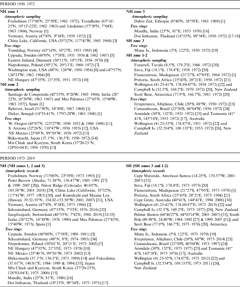
Notes: [1] = Nydal and Lövseth (Reference Nydal and Lövseth1996); [2] = Levin and Kromer (Reference Levin and Kromer2004); [3] = Berger et al. (Reference Berger, Fergusson and Libby1965) and Berger and Libby (Reference Berger and Libby1966, Reference Berger and Libby1967, Reference Berger and Libby1968, Reference Berger and Libby1969); [4] = Svarva et al. (Reference Svarva, Grootes, Seiler, Stene, Thun, Værnes and Nadeau2019); [5] = Olsson and Possnert (Reference Olsson and Possnert1992); [6] = Kudsk et al. (Reference Kudsk, Olsen, Nielsen, Fogtmann-Schulz, Knudsen and Karoff2018); [7] = Rakowski et al. (Reference Rakowski, Nadeau, Nakamura, Pazdur, Paweczyk and Piotrowska2013); [8] = Stuiver et al. (Reference Stuiver, Reimer and Braziunas1998); [9] = Grootes et al. (Reference Grootes, Farwell, Schmidt, Leach and Stuiver1989); [10] = Hertelendi and Csongor (Reference Hertelendi and Csongor1982); [11] = Cain et al. (Reference Cain, Griffin, Druffel-Rodriguez and Druffel2018); [12] = Damon et al. (Reference Damon, Cheng and Linick1989); [13] = Beramendi-Orosco et al. (Reference Beramendi-Orosco, Johnson, Noronha, González-Hernández and Villanueva-Díaz2018); [14] = Yamada et al. (Reference Yamada, Yasuike and Komura2005); [15] = Park et al. (Reference Park, Kim, Cheoun, Kim, Youn, Liu and Kim2002); [16] = Murphy et al. (Reference Murphy, Lawson, Fink, Hotchkis, Hua, Jacobsen, Smith and Tuniz1997); [17] = Hua et al. (Reference Hua, Barbetti, Jacobsen, Zoppi and Lawson2000); [18] = Hua et al. (Reference Hua, Barbetti and Zoppi2004); [19] = Hua et al. (Reference Hua, Barbetti, Levchenko, D’Arrigo, Buckley and Smith2012); [20] = Manning et al. (Reference Manning, Lowe, Melhuish, Sparks, Wallace, Brenninkmeijer and McGrill1990); [21] = Vogel and Marais (Reference Vogel and Marais1971); [22] = Turnbull et al. (Reference Turnbull, Mikaloff Fletcher, Ansell, Brailsford, Moss, Norris and Steinkamp2017); [23] = Ancapichún et al. (Reference Ancapichún, De Pol-Holz, Christie, Santos, Collado-Fabbri, Garreaud, Lambert, Orfanoz-Cheuquelaf, Rojas, Southon, Turnbull and Creasman2021); [24] = Santos et al. (Reference Santos, Linares, Lisi and Tomazello Filho2015); [25] = Hua et al. (Reference Hua, Barbetti, Zoppi, Chapman and Thomson2003); [26] = Turney et al. (Reference Turney, Palmer, Maslin, Hogg, Fogwill, Southon, Fenwick, Helle, Wilmshurst, McGlone, Bronk Ramsey, Thomas, Lipson, Beaven, Jones, Andrews and Hua2018); [27] = Meijer et al. (Reference Meijer, Pertuisot and van der Plicht2006); [28] = Graven et al. (Reference Graven, Guilderson and Keeling2012a); [29] = Turnbull et al. (Reference Turnbull, Lehman, Miller, Sparks, Southon and Tans2007), Lehman et al. (Reference Lehman, Miller, Wolak, Southon, Tans, Montzka, Sweeney, Andrews, LaFranchi, Guilderson and Turnbull2013), and Lehman and Miller (Reference Lehman and Miller2019); [30] = Berger et al. (Reference Berger, Jackson, Michael and Suess1987); [31] = Graven et al. (Reference Graven, Guilderson and Keeling2012b); [32] = Levin and Kromer (Reference Levin and Kromer2004), and Hammer and Levin (Reference Hammer and Levin2017); [33] = Emmenegger et al. (Reference Emmenegger, Leuenberger and Steinbacher2020); [34] = Levin and Kromer (Reference Levin and Kromer1997); [35] = Xu et al. (Reference Xu, Cook, Cresswell, Dunbar, Freeman, Hastie, Hou, Jacobsson, Naysmith and Sanderson2015); and [36] = Levin et al. (Reference Levin, Kromer and Francey1996, Reference Levin, Kromer and Francey1999, Reference Levin, Kromer, Steele and Porter2011).

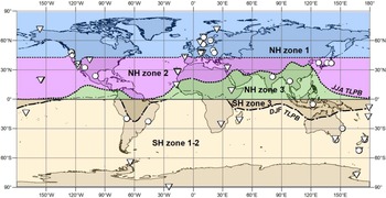
Figure 1 World map showing the zones and locations of atmospheric CO2 sampling (triangles) for 14C analysis and Δ14C tree-ring records (circles) used for our compilation. The mean positions of the TLPB during December–February (DJF) and June–August (JJA) are based on the NCEP/NCAR sea level pressure data (Kalnay et al. Reference Kalnay, Kanamitsu, Kistler, Collins, Deaven, Gandin, Iredell, Saha, White, Woollen, Zhu, Chelliah, Ebisuzaki, Higgins, Janowiak, Mo, Ropelewski, Wang, Leetmaa, Reynolds, Jenne and Joseph1996) for 1949–2019.
ZONAL ATMOSPHERIC Δ14C AND BOUNDARIES
As a result of aboveground nuclear detonations mostly in the NH, the majority of bomb 14C resided in the northern stratosphere during the years of intensive atmospheric nuclear testing and approximately one year after the 1963 Nuclear Test Ban Treaty (1962–1964) (Telegadas Reference Telegadas1971; Hesshaimer and Levin Reference Hesshaimer and Levin2000; Naegler and Levin Reference Naegler and Levin2006). Bomb 14C was injected into the troposphere through the mid- to high-latitude tropopause gaps during the springtime of each hemisphere. The seasonality of this exchange led to a 14C disequilibrium between the stratosphere and the troposphere during the early 1960s (Hesshaimer and Levin Reference Hesshaimer and Levin2000), which was employed for constraining parameters related to atmospheric transport across the tropopause (Hesshaimer Reference Hesshaimer1997; Levin et al. Reference Levin, Naegler, Kromer, Diehl, Francey, Gomez-Pelaez, Steele, Wagenbach, Weller and Worthy2010). The excess-14C injection from the stratosphere also created large 14C gradients between tropospheric high and low latitudes, and between the northern and southern troposphere during ca. 1955–1967 (Hua and Barbetti Reference Hua and Barbetti2007; Hua et al. Reference Hua, Barbetti, Levchenko, D’Arrigo, Buckley and Smith2012), which are valuable for modeling tropospheric air mass transport. Excess 14C was subsequently transferred southwards and the spatial distribution of tropospheric radiocarbon during this period is strongly influenced by atmospheric transport and mixing through the large-scale wind systems including monsoon circulation (Hua and Barbetti Reference Hua and Barbetti2007; Levin et al. Reference Levin, Naegler, Kromer, Diehl, Francey, Gomez-Pelaez, Steele, Wagenbach, Weller and Worthy2010; Hua et al. Reference Hua, Barbetti, Levchenko, D’Arrigo, Buckley and Smith2012). This spatial distribution seems to be further characterised by 5 zones of different Δ14C levels (NH zones 1, 2, and 3, and SH zones 3 and 1–2; see Figure 1) that decrease from north to south (Hua et al. Reference Hua, Barbetti and Rakowski2013). NH zone 1 in northern mid- to high latitudes, where most of the excess 14C from the stratosphere was injected into the troposphere (e.g., Levin et al. Reference Levin, Kromer, Schoch-Fischer, Bruns, Münnich, Berdau, Vogel and Münnich1985; Nydal and Gislefoss Reference Nydal and Gislefoss1996), had the highest Δ14C values during this period. Meanwhile, at the same time, SH zone 1–2 covering most of the SH recorded the lowest Δ14C values, and the other zones recorded intermediate Δ14C levels. The intra-hemispheric differences in atmospheric Δ14C were substantially reduced in the late 1960s and early 1970s (Telegadas Reference Telegadas1971; Manning et al. Reference Manning, Lowe, Melhuish, Sparks, Wallace, Brenninkmeijer and McGrill1990) as a result of atmospheric mixing, and from 1973 onwards there have been similar Δ14C values between locations within each hemisphere (Hua et al. Reference Hua, Barbetti and Rakowski2013). Similar to Hua et al. (Reference Hua, Barbetti and Rakowski2013), in this current study we employed the five-zone pattern of atmospheric Δ14C, which broadly reflects major zones of atmospheric circulation, with different zonal Δ14C levels for 1950–1972 and very similar zonal Δ14C values in each hemisphere for 1973–2019.
Figure 1 shows the zonal boundaries. The boundary between NH zone 2 and NH zone 3 is defined as the mean position of the convergence of northeasterly trade winds from the northern subtropics and winds from the northern and southern tropics during June, July and August (JJA). This convergence, known as the Inter-Tropical Convergence Zone (ITCZ), is associated with a low-pressure band (tropical low pressure belt (TLPB); Ancapichún et al. Reference Ancapichún, De Pol-Holz, Christie, Santos, Collado-Fabbri, Garreaud, Lambert, Orfanoz-Cheuquelaf, Rojas, Southon, Turnbull and Creasman2021). However, as the ITCZ is a marine phenomenon and is not well defined over the continents (e.g., Vuille et al Reference Vuille, Burns, Taylor, Cruz, Bird, Abbott, Kanner, Cheng and Novello2012; Marsh et al. Reference Marsh, Bruno, Fritz, Baker, Capriles and Hastorf2018), in this paper we use TLPB instead of ITCZ concerning the wind convergence associated with the low-pressure band. During December, January and February (DJF), the TLPB has a southward position, which is the convergence of winds from the northern tropics and easterly winds from the southern tropics and subtropics (Hogg et al. Reference Hogg, Heaton, Hua, Palmer, Turney, Southon, Bayliss, Blackwell, Boswijk, Bronk Ramsey, Pearson, Petchey, Reimer, Reimer and Wacker2020; Ancapichún et al. Reference Ancapichún, De Pol-Holz, Christie, Santos, Collado-Fabbri, Garreaud, Lambert, Orfanoz-Cheuquelaf, Rojas, Southon, Turnbull and Creasman2021). The mean DJF position of the TLPB in the eastern Pacific, the eastern Atlantic and most of Central Africa is located in the NH. Therefore, for these regions SH zone 3 was not defined and the Equator was employed as the boundary between NH zone 3 and SH zone 1–2. The mean DJF position of the TLPB in the western Pacific, the Indian Ocean and South America is located in the SH and was used as the boundary between SH zone 3 and SH zone 1–2. It is worth noting that lower Δ14C values over the Southern Ocean, related to air-sea gas exchange with 14C-depleted surface ocean water that is generated by upwelling of intermediate and deeper ocean waters (ca. 3–6‰ during the late 1980s–the 2000s) compared to SH sub-tropical and temperate sites are well documented (Levin et al. Reference Levin, Naegler, Kromer, Diehl, Francey, Gomez-Pelaez, Steele, Wagenbach, Weller and Worthy2010; Graven et al. Reference Graven, Guilderson and Keeling2012b; Turney et al. Reference Turney, Palmer, Hogg, Fogwill, Jones, Bronk Ramsey, Fenwick, Grierson, Wilmshurst, O’Donnell, Thomas and Lipson2016) and there is some suggestion that it would be appropriate to define these areas as two separate zones. However, for the intended application of dating terrestrial materials, this applies only to a very limited subset of locations south of ca. 50°S. In addition, only a small amount of data is currently available for this region and highlights the need for further work over the Southern Ocean. Therefore, in the current compilation, results from SH zones 1 and 2 are binned into a single Δ14C zone, SH zone 1–2.
The new tree-ring record from Irruputuncu, Altiplano, Chile at 20°S, 68°W (Ancapichún et al. Reference Ancapichún, De Pol-Holz, Christie, Santos, Collado-Fabbri, Garreaud, Lambert, Orfanoz-Cheuquelaf, Rojas, Southon, Turnbull and Creasman2021) is located close to the western edge of the South American “U-shaped” boundary between SH zone 3 and SH zone 1–2 derived from the NCEP/NCAR sea level pressure data (Kalnay et al. Reference Kalnay, Kanamitsu, Kistler, Collins, Deaven, Gandin, Iredell, Saha, White, Woollen, Zhu, Chelliah, Ebisuzaki, Higgins, Janowiak, Mo, Ropelewski, Wang, Leetmaa, Reynolds, Jenne and Joseph1996) (Figure 1). Despite a minor portion of the air parcels (21%) reaching Irruputuncu from the Amazon basin (SH zone 3), its tree-ring Δ14C values are similar to those from Wellington, New Zealand (Ancapichún et al. Reference Ancapichún, De Pol-Holz, Christie, Santos, Collado-Fabbri, Garreaud, Lambert, Orfanoz-Cheuquelaf, Rojas, Southon, Turnbull and Creasman2021) located in SH zone 1–2. Thus, appropriate development of new tree-ring records from low to mid-latitude regions is necessary as a means to better define the areas affected by changes in the mean TLPB position.
The boundary between NH zone 1 and NH zone 2 was previously defined based on limited 14C records in mid- to high northern latitudes during the bomb peak period. According to Hua and Barbetti (Reference Hua and Barbetti2004) and Hua et al. (Reference Hua, Barbetti and Rakowski2013), this boundary around 40°N is located south of China Lake (CL; 35°32'N, 117°41'W) but north of Santiago de Compostela (42°53'N, 8°26'W). With the recent availability of the tree-ring record from western Oregon, USA (45°07'N, 123°27'W; 1960–1969; Cain et al. Reference Cain, Griffin, Druffel-Rodriguez and Druffel2018) and the inclusion of a short tree-ring data set from Washington state, USA (47°57'N, 124°33'W; 1962–1964; Grootes et al. Reference Grootes, Farwell, Schmidt, Leach and Stuiver1989), the position of this boundary in northwestern America can be refined.
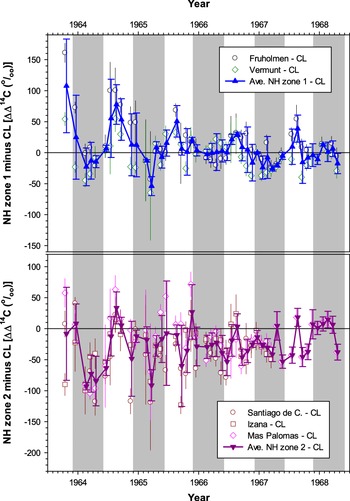
Hua and Barbetti (Reference Hua and Barbetti2004) suggested that the CL atmospheric record (1963–1968) belonged to NH zone 1, based on the fact that the average of monthly Δ14C differences between CL and NH zone 1 data, and between CL and NH zone 2 data are negligible and large, respectively. It is worth noting that higher Δ14C values of the CL record compared to those of other atmospheric data sets at similar latitudes in NH zone 2 are not likely due to influences of nearby Nevada bomb tests on CL (see later discussion).
Figure 2 shows monthly Δ14C differences between NH zone 1 and CL, and between NH zone 2 and CL. The CL Δ14C values are similar to NH zone 1 values and higher than NH zone 2 values mostly during winter-spring (grey stripes in Figure 2), but lower than NH zone 1 values and similar to NH zone 2 values during summer-autumn (white stripes in Figure 2) except for late 1967–1968 due to reduced Δ14C differences between regions in the late 1960s. These observations support large seasonal variations of the polar jet in north-western America as discussed in the literature (e.g., Barton and Ellis Reference Barton and Ellis2009; Pena-Ortiz et al. Reference Pena-Ortiz, Gallego, Ribera, Ordonez and Alvarez-Castro2013). They also indicate that during the bomb peak period the polar jet moved southwards as far as south of CL in winter-spring and CL received air masses from the north containing higher Δ14C values than southern air-masses, while in summer-autumn the polar jet travelled northwards resulting in a contribution of the southern air masses to CL.

Figure 2 Monthly Δ14C differences between atmospheric records in NH zones 1 and 2, and China Lake (CL). Data sources of these atmospheric records are Berger et al. (Reference Berger, Fergusson and Libby1965) and Berger and Libby (Reference Berger and Libby1966, Reference Berger and Libby1967, Reference Berger and Libby1968, Reference Berger and Libby1969) for CL, Levin and Kromer (Reference Levin and Kromer2004) for Vermunt, and Nydal and Lövseth (Reference Nydal and Lövseth1996) for Fruholmen, Santiago de Compostela, Izaña and Mas Palomas. Grey and white stripes represent winter–spring and summer–autumn, respectively.
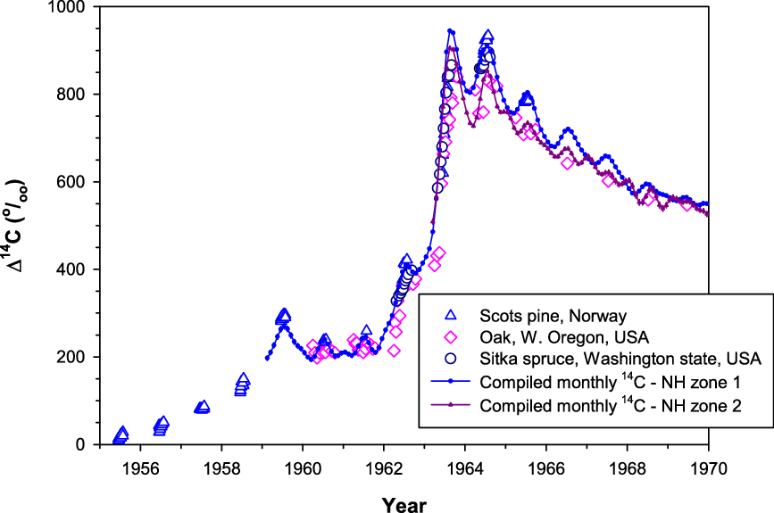
In contrast, an oak tree from western Oregon, located northwest of CL, with radial growth during spring–late autumn has Δ14C values close to those of NH zone 2 rather than NH zone 1 (Cain et al. Reference Cain, Griffin, Druffel-Rodriguez and Druffel2018; Figure 3). The authors used the Pacific North American (PNA) index, representing a record of large-scale weather patterns that describe the placement of the polar and sub-tropical jets, to explain some relatively low values of their tree-ring Δ14C. They showed that monthly PNA index values for March–June were negative in 1962–1964, coinciding with relatively low tree-ring Δ14C values during April–June of 1962–1964. This suggests during this period both the polar and sub-tropical jets moved northwards and their tree rings reflected carbon uptake from air masses coming from the south containing lower bomb Δ14C values.

Figure 3 Tree-ring Δ14C values from Scots pine (Norway; Svarva et al. Reference Svarva, Grootes, Seiler, Stene, Thun, Værnes and Nadeau2019), oak (western Oregon, USA; Cain et al. Reference Cain, Griffin, Druffel-Rodriguez and Druffel2018) and Sitka spruce (Washington state, USA; Grootes et al. Reference Grootes, Farwell, Schmidt, Leach and Stuiver1989) versus compiled monthly Δ14C data for NH zones 1 and 2 derived from atmospheric records (see discussions later on the construction of these compiled data).
Furthermore, Δ14C values of Sitka spruce tree rings from Washington state (Grootes et al. Reference Grootes, Farwell, Schmidt, Leach and Stuiver1989) located north of the Oregon tree rings are similar to NH zone 1 values based on atmospheric records (Figure 3). Large seasonal variation in the position of the polar jet in north-western America discussed above means that the boundary between NH zone 1 and NH zone 2 varies seasonally. However, with the Δ14C data during the bomb peak currently available for this region (CL atmospheric record, and Oregon and Washington tree-ring data) and for our practical purposes, the boundary between NH zone 1 and NH zone 2 is considered to be located between the two tree-ring sites and south of CL (see Figure 1). More tree-ring records in north-western America are useful for further refinement of the position of the boundary between NH zone 1 and NH zone 2 in this region.
One may argue that higher Δ14C values of the CL record (1963–1968) compared to those of other atmospheric data sets at similar latitudes, belonging to NH zone 2, are due to influences of Nevada bomb tests on CL. There were quite a number of low-yield atmospheric nuclear bomb tests at Nevada (36.6–37.2°N, 115.9–116.4°W) during 1951–1958 and 1962 (UNSCEAR, 2000). In 1962, there were only 4 atmospheric nuclear weapon tests in July with a detonation yield ranging from 5 to 20 kton each. The Nevada test sites are located northeast of CL (35°32'N, 117°41'W). Low-yield atmospheric nuclear bomb tests have a tendency to substantially contribute to local/regional areas (e.g., Enting Reference Enting1982). If this were the case for these Nevada bomb tests in 1962, their contribution to CL would be clearly seen in 1962 and approximately one year after the tests (i.e., 1963). This is because atmospheric transport is quite fast, which is ca. 1 year from northern mid-latitudes to northern tropics based on the timing of the bomb Δ14C peaks in atmospheric sampling (August 1963 in Vermunt, Austria [Levin and Kromer Reference Levin and Kromer2004] and July 1964 in Dakar, Senegal [Nydal and Lövseth Reference Nydal and Lövseth1996]) for example. However, the two earliest CL Δ14C values available in 1963 are similar to NH zone 2 values (Figure 2). In addition, CL Δ14C values are higher than NH zone 2 values during winter-spring seasons in 1964–1965 (Figure 2), 2–3 years after the tests. These indicate that relatively high CL Δ14C values during the bomb peak period are unlikely due to the contribution of the 1962 Nevada nuclear bomb tests.
COMPILATION METHODS
Timing of Tree-Ring Growth Seasons
Growth seasons of different tree-ring species in different regions employed in our compilation are not identical, but they are similar (e.g., Hua et al. Reference Hua, Barbetti, Levchenko, D’Arrigo, Buckley and Smith2012; Cain et al. Reference Cain, Griffin, Druffel-Rodriguez and Druffel2018; Turney et al. Reference Turney, Palmer, Maslin, Hogg, Fogwill, Southon, Fenwick, Helle, Wilmshurst, McGlone, Bronk Ramsey, Thomas, Lipson, Beaven, Jones, Andrews and Hua2018; Svarva et al. Reference Svarva, Grootes, Seiler, Stene, Thun, Værnes and Nadeau2019; Ancapichún et al. Reference Ancapichún, De Pol-Holz, Christie, Santos, Collado-Fabbri, Garreaud, Lambert, Orfanoz-Cheuquelaf, Rojas, Southon, Turnbull and Creasman2021). The duration of growing seasons can also vary slightly from one year to another. However, tree growth follows a similar pattern of slow increment at the start (early spring to early summer) and end (late summer to autumn) of a growing season, while fast increment occurs during summer (Grootes et al. Reference Grootes, Farwell, Schmidt, Leach and Stuiver1989; Hua et al. Reference Hua, Barbetti, Jacobsen, Zoppi and Lawson2000; Turnbull et al. Reference Turnbull, Mikaloff Fletcher, Ansell, Brailsford, Moss, Norris and Steinkamp2017; Cain et al. Reference Cain, Griffin, Druffel-Rodriguez and Druffel2018; Kudsk et al. Reference Kudsk, Olsen, Nielsen, Fogtmann-Schulz, Knudsen and Karoff2018; Svarva et al. Reference Svarva, Grootes, Seiler, Stene, Thun, Værnes and Nadeau2019). This also applies to tropical tree rings used in the current compilation for which most growth occurs in summer rainy seasons (e.g., Hua et al. Reference Hua, Barbetti, Jacobsen, Zoppi and Lawson2000, Reference Hua, Barbetti, Levchenko, D’Arrigo, Buckley and Smith2012). In addition, for each annual ring, wood material away from the ring boundaries is usually sampled for 14C analysis (e.g., Hua et al. Reference Hua, Barbetti, Worbes, Head and Levchenko1999, Reference Hua, Barbetti, Levchenko, D’Arrigo, Buckley and Smith2012) to avoid potential cross-ring-boundary issues. Thus, the material of each ring selected for 14C analysis is mainly the portion of wood growing in summer in both hemispheres (May–August or the middle of the current year for the NH, and November–February or the beginning of the following year for the SH). This simple approach allows for estimation of hemispheric and global summer means from tree-ring Δ14C values and associated atmospheric Δ14C values in addition to the construction of the zonal estimates.
Compiled Data
Our compilation provides both summer and monthly results. The summer data were derived from atmospheric sampling and tree-ring records using a simple averaging method. Monthly data were primarily based on atmospheric sampling, with tree-ring data only used when atmospheric CO2 data were not available, mostly during the pre-bomb and early bomb period. A curve fitting method was employed to construct monthly results.
Summer Data
Zonal, hemispheric, and global summer data sets were compiled. Five separate zonal data sets (3 for the NH and 2 for the SH) were constructed for the period 1950–1972. Due to similar Δ14C values between locations in each hemisphere from 1973 onwards (Hua et al. Reference Hua, Barbetti and Rakowski2013), 3 identical zonal data sets for the NH and 2 identical zonal data sets for the SH were compiled. We modified the methods employed by Hua et al. (Reference Hua, Barbetti and Rakowski2013) for the construction of these summer data sets, which are described below.
The mean value for summers (May–August for the NH (Hua and Barbetti Reference Hua and Barbetti2004; Hammer and Levin Reference Hammer and Levin2017) and November–February for the SH (Hua and Barbetti Reference Hua and Barbetti2004)) for an atmospheric Δ14C record for a particular year was calculated only if there were data available for at least 3 out of 4 months for the season. The mean summer value for a particular zone in a particular year was then calculated with weight being the uncertainty associated with the summer mean of the individual record (atmospheric sampling or tree rings).
As the surface areas covered by the three NH zones are different in size (Figure 1), summer mean values for the NH for the period 1950–1972 were calculated from the 3 zonal summer means, with weights being the percentages of zonal surface areas (ca. 17%, 46%, and 37% for NH zones 1, 2, and 3, respectively). The same approach was employed for the calculation of summer mean values for the SH for 1950–1972 with the percentages of zonal surface areas for SH zones 3 and 1–2 being ca. 15% and 85%, respectively. For the period 1973–2019, hemispheric summer mean values are actual zonal summer values.
Two zonal (SH zones 3 and 1–2) data sets for boreal summers were also compiled to construct the global boreal summer data set. For 1950–1972, the global boreal summer means were calculated using the 5 zonal (boreal summer) data sets with weights being the percentages of zonal surface areas mentioned above. For the period 1973–2019, the global boreal summer means were calculated using the 2 hemispheric data sets for boreal summers.
Monthly Data
Five zonal monthly data sets were constructed using the ccgcrv curve fitting method (Thoning et al. Reference Thoning, Tans and Komhyr1989) to output smooth curves at monthly resolution. The data used for the curve fitting were primarily atmospheric records. When atmospheric records were not available (e.g., mostly the pre-bomb and early bomb period), average zonal summer data and/or sub-annual tree-ring data were employed. In addition, to avoid possible discontinuities between our NH monthly data sets and IntCal20 curve (Reimer et al. Reference Reimer, Austin, Bard, Bayliss, Blackwell, Bronk Ramsey, Butzin, Cheng, Edwards, Friedrich, Grootes, Guilderson, Hajdas, Heaton, Hogg, Hughen, Kromer, Manning, Muscheler, Palmer, Pearson, van der Plicht, Reimer, Richards, Scott, Southon, Turney, Wacker, Adolphi, Büntgen, Capano, Fahrni, Fogtmann-Schulz, Friedrich, Köhler, Kudsk, Miyake, Olsen, Reinig, Sakamoto, Sookdeo and Talamo2020) when they are used together for dating, we included the raw IntCal20 data for 1941–1950 in our curve fitting. The same approach was applied for the construction of the SH monthly data sets by including the raw SHCal20 data for 1941–1950 (Hogg et al. Reference Hogg, Heaton, Hua, Palmer, Turney, Southon, Bayliss, Blackwell, Boswijk, Bronk Ramsey, Pearson, Petchey, Reimer, Reimer and Wacker2020).
To develop the smooth curves, all data for a given zonal data set were compiled, then a smooth curve was created following the method of Turnbull et al. (Reference Turnbull, Mikaloff Fletcher, Ansell, Brailsford, Moss, Norris and Steinkamp2017). Each data set was split into six time intervals (1941–1955, 1954–1966, 1965–1973, 1972–1990, 1989–2006, and 2005–2020) to allow the seasonal cycle and long-term trend to vary through time. The parameters used in the ccgcrv curve fitting are interval = 365, cutoff1=180 and cutoff2 = 1900 for the early periods when only tree-ring data were available, and interval = 14, cutoff1=180 and cutoff2 = 667 for the other periods. A Monte Carlo method with 1000 iterations was used to create a smooth curve for each time interval, with uncertainty assigned from the scatter of the Monte Carlo simulation. For each of the 1000 simulations, the 14C value for each date sampled is re-assigned randomly according to the normal distribution described by the mean and reported standard deviation of the measurement. A curve is fitted to each of the 1000 simulations, then the mean and standard deviation are calculated for each time step from the spread of the 1000 fitted curves. In this simulation, input data was at its native resolution (i.e., every raw data point was included), and the fitted curves were output at monthly resolution.
Finally, all six time intervals were spliced together, averaging across the overlap periods, to produce a smooth curve fit for the entire period. Alternative curve fitting methods do allow varying seasonal cycles (e.g., Pickers and Manning Reference Pickers and Manning2015), but require gap filling with interpolated data, which introduces a different set of biases.
For the pre-bomb and early bomb period and a short period 1970–1972 in NH zone 3 when only tree-ring data were available (except for SH zone 1–2 where atmospheric data were available), it is not possible to derive a seasonal cycle from the (summertime only) tree-ring data. It is also inappropriate to assign the seasonal cycle for the latter time period, as it is clear that the Δ14C seasonal cycle changed dramatically with the inputs of bomb 14C. Therefore, we chose not to assign any seasonal cycle to these periods, instead of interpolating the interannual trend to provide monthly Δ14C values.
RESULTS AND DISCUSSION
Many plants and some animals depend on the carbon formed during the summer growing season, making the compiled zonal summer data sets appropriate for use in radiocarbon dating of these sample types. However, for other plants and vegetation, whose main growing seasons are different such as early-spring for leaves, autumn plants/seeds and winter wheat/rice, the zonal summer data sets are not useful for dating of these materials. Vegetation in the aseasonal tropics between ∼5°N and ∼5°S, growing almost all year round, is also in this category. In addition, humans and animals, who consume foods mostly imported from around the globe, may not be accurately dated using the zonal summer data sets. We, therefore, take a simple and consistent approach, and recommend the compiled zonal monthly data sets should be used for dating of all recent samples.
Similar to the previous compilations (Tans Reference Tans1981; Hua and Barbetti Reference Hua and Barbetti2004; Hua et al. Reference Hua, Barbetti and Rakowski2013; Graven et al. Reference Graven, Allison, Etheridge, Hammer, Keeling, Levin, Meijer, Rubino, Tans, Trudinger, Vaughn and White2017), we aimed to provide compiled Δ14C data sets with annual resolution for use in carbon cycle modeling. Summer data sets were chosen as their raw data were the only data available for the whole period of interest, 1950–2019. In addition, an advantage of these summer data sets is that they can be extended back in time using compatible tree-ring based IntCal20 or SHCal20 data, if longer data sets are required for modeling studies. The zonal monthly data sets were constructed for dating purposes as discussed above. However, they can be used for carbon cycle modeling if it requires higher temporal resolution.
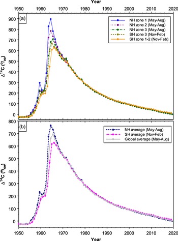
Compiled zonal atmospheric Δ14C data sets for NH zones 1, 2, and 3 for boreal summers (May–August) for the period 1950–2019 are presented in Supplementary Table S1a, while compiled zonal atmospheric Δ14C data sets for SH zones 3 and 1–2 for austral summers (November–February) are reported in Supplementary Table S1b. All the compiled zonal Δ14C data sets are illustrated in Figure 4a. Compiled hemispheric Δ14C data sets for boreal and austral summers are also reported in Supplementary Table S1a and Table S1b, respectively, while the compiled global atmospheric Δ14C data set for boreal summers is presented in Supplementary Table S1c. The compiled hemispheric and global atmospheric Δ14C data sets for 1950–2019 are also depicted in Figure 4b.

Our compiled summer Δ14C data sets have good agreement with those of Hua et al. (Reference Hua, Barbetti and Rakowski2013) for the overlapping periods (1950–2010 for the NH and 1950–2011 for the SH; see Supplementary Figures S1a–h). The compilation by Graven et al. (Reference Graven, Allison, Etheridge, Hammer, Keeling, Levin, Meijer, Rubino, Tans, Trudinger, Vaughn and White2017) for 1950–2015 consists of annual Δ14C data for 3 different regions, NH north of 30°N (NH>30°N), 30°N–30°S and SH south of 30°S (SH>30°S), with the timing of each data point being in the middle of a year. For ease of comparison with our compiled data for the SH with each data point being the beginning of the following year, the compiled data for 2 regions 30°N–30°S and SH>30°S from Graven et al. (Reference Graven, Allison, Etheridge, Hammer, Keeling, Levin, Meijer, Rubino, Tans, Trudinger, Vaughn and White2017) were linearly interpolated (see Supplementary Figures S2c–d). In general, we find good concordance between our and their compiled Δ14C data (Supplementary Figures S2a–d), although the spatial coverage of the study regions in these two studies are not the same.
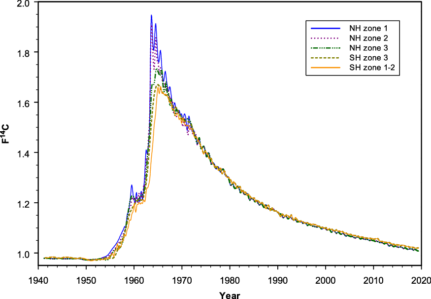
Compiled zonal data sets at monthly resolution for 1941–2019, in Δ14C and F14C (Reimer et al. Reference Reimer, Brown and Reimer2004), are reported in Supplementary Tables S2a–e. These data in F14C are also shown in Figure 5. The ccgcrv curve fitting method used for the compilation of monthly data sets in this study has a couple of advantages compared to the weighted average methods used by Hua et al. (Reference Hua, Barbetti and Rakowski2013). First, the curve fitting method smooths the noise associated with the relatively large uncertainties assigned to individual measurements, resulting in smoother compiled data with clear seasonal cycles for the periods covered by atmospheric Δ14C records (Figures 5 and 6a–e). Second, the compiled extended monthly data sets of Hua et al. (Reference Hua, Barbetti and Rakowski2013) have different temporal resolutions with monthly data for the periods covered by atmospheric Δ14C records and annual summer data outside these periods. Meanwhile, the compiled data sets in the current study have a monthly resolution for the whole period of 1941–2019 (see Figures 6a–e; Supplementary Tables S2a–e). Thus, the curve fitting method used in the present study resulted in improved zonal monthly data sets and consequently improved radiocarbon dating of recent terrestrial samples.


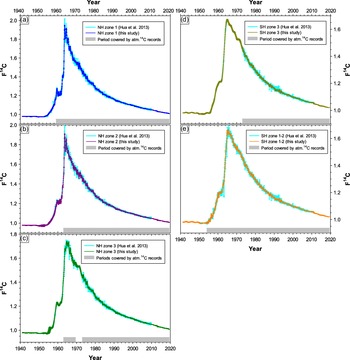
Figure 6 Our compiled monthly atmospheric F14C curves versus those of Hua et al. (Reference Hua, Barbetti and Rakowski2013).
Good agreement between the compiled monthly data sets and IntCal20 or SHCal20 is observed for the overlapping period (1941–1950) (Supplementary Figures S3a–e), indicating the continuity between these data sets when they are used together for radiocarbon dating. We recommend that when calibrations span the pre- and post-bomb periods, users replace the IntCal20 or SHCal20 data for 1941–1950 with the compiled monthly data for 1941–1950 to avoid discontinuities between the datasets.
The compiled monthly data sets for the NH zones in this study agree well with those of Hua et al. (Reference Hua, Barbetti and Rakowski2013) for the overlapping period (1950–2009) (Figures 6a–c). It should be noted that the Monte Carlo simulation associated with the curve fitting method assigns smaller uncertainties than the standard deviations that were assigned in the previous study.
For the SH zones, a similar pattern is observed except during 1990–1993 (Figures 6d–e). With the revision of the Wellington atmospheric Δ14C record for 1990–1993 (Turnbull et al. Reference Turnbull, Mikaloff Fletcher, Ansell, Brailsford, Moss, Norris and Steinkamp2017), our compiled monthly F14C data for the SH zones for this period are lower than those of the 2013 data (Figures 6d–e). This means anomalously high F14C values for this period, which previously appeared in the 2013 data for the SH zones, no longer exist in our compiled monthly data. Similarly, anomalously high Δ14C values for 1990–1993, previously appearing in the compiled summer data of Hua et al. (Reference Hua, Barbetti and Rakowski2013) for the SH zones, are also not evident in our compiled summer data (see Supplementary Figures S1d–e).
The compiled monthly F14C data are mostly based on atmospheric records, but they are derived from tree-ring records when atmospheric sampling is not available (Figures 6a–e). The use of tree-ring data to extend the compiled monthly atmospheric-based data is an advantage. However, tree rings do not fully represent atmospheric Δ14C levels when these levels change substantially and quickly, although tree-ring Δ14C follows atmospheric Δ14C very well with a delay of no more than ca. 2 weeks for Washington Sitka spruce (Grootes et al. Reference Grootes, Farwell, Schmidt, Leach and Stuiver1989) or 5–6 weeks for Tasmanian Huon pine (Hua et al. Reference Hua, Barbetti, Jacobsen, Zoppi and Lawson2000). For example, atmospheric F14C (and consequently Δ14C) in NH zone 1 peaks in 1963 (Figure 5) but tree-ring Δ14C in this zone reaches its maximum in 1964 (Figure 4a). Another example, which can be seen in Figure 3, indicates that sub-annual tree-ring Δ14C for the NH zones 1 and 2 during 1963–1964 do not cover the full ranges of their associated atmospheric Δ14C values. These differences are likely due to growing seasons, which are only a portion of a year, seasonal averaging or insufficient sampling resolution for tree rings. Substantial changes in atmospheric Δ14C levels occur during the early bomb period and the bomb peak period. During these periods, needles/leaves of early spring, autumn plants/seeds and winter wheat/rice incorporate atmospheric Δ14C values at the time of growth, which may be substantially different from those of annual and/or sub-annual tree rings. This issue, therefore, should be considered or recognized when dating such samples for the periods that the compiled monthly 14C data are derived from tree-ring records such as 1955–1959 for NH zone 1, 1955–1963 for NH zones 2 and 3, and especially 1955–1972 for SH zone 3 (see Figures 6a–d).
After reaching its peak levels, atmospheric Δ14C in the NH and SH has decreased since 1963–1964 and 1964–1965, respectively. Decreases in atmospheric Δ14C from the mid-1960s to mid-1980s are mainly due to rapid exchange between the atmosphere and the biosphere and oceans (Oeschger et al. Reference Oeschger, Siegenthaler, Schotterer and Gugelmann1975; Druffel and Suess Reference Druffel and Suess1983; Levin and Hesshaimer Reference Levin and Hesshaimer2000), while combustion of fossil fuels free of 14C is the main causal factor for the Δ14C decline since the late 1980s and early 1990s (Levin et al. Reference Levin, Naegler, Kromer, Diehl, Francey, Gomez-Pelaez, Steele, Wagenbach, Weller and Worthy2010; Graven et al. Reference Graven, Guilderson and Keeling2012a). Since the early and late 2000s, the atmospheric Δ14C values have been lower than those of the surface waters in the North and South Pacific Gyres, respectively, indicating the oceans might become a net 14C source (instead of a net 14C sink) of the atmosphere (Andrews et al. Reference Andrews, Siciliano, Potts, DeMartini and Covarrubias2016, Reference Andrews, Prouty and Cheriton2021; Wu et al. Reference Wu, Fallon, Cantin and Lough2021).
The last data points in our compiled monthly data at 2019.375 have respective F14C values of 1.0084 and 1.0195 for the NH and SH (see Supplementary Tables 2a–e), which are very close to the pre-bomb F14C value of slightly lower than 1. This indicates that clean-air F14C is likely to reach the pre-bomb value in the early 2020s, which is similar to the estimation of Graven (Reference Graven2015) and Sierra (Reference Sierra2018). If this occurs, radiocarbon dating of a single terrestrial sample having F14C lower than 1 delivers two possible ages: pre-1955 and the early 2020s or after. Graven (Reference Graven2015) discussed issues of radiocarbon dating of single samples with different scenarios of fossil-fuel emissions, suggesting that the radiocarbon method may not provide definitive ages for samples up to 2000 years old under a worst-case, high-emission scenario from fossil fuels. To avoid these issues, radiocarbon dating of a series of samples in sequence with known chronological ordering (e.g., samples from a sediment profile or along the growth axis of a tree) combined with other isotopic studies should be employed. Constraints in the chronological ordering of measured radiocarbon ages (or F14C values) of the sequence samples give a much better indication (than that of a single sample) on their calendar ages, resulting in more definite ages for each sample in the sequence (e.g., Goslar et al. Reference Goslar, van der Knaap, Hicks, Andrič, Czernik, Goslar, Räsänen and Hyötylä2005; Yeloff et al. Reference Yeloff, Bennett, Blaauw, Mauquoy, Sillasoo, van der Plicht and van Geel2006; Hua Reference Hua2009; Santini et al. Reference Santini, Hua, Schmitz and Lovelock2013). As fossil fuels are not only depleted in 14C (F14C = 0 and Δ14C = –1000‰) but also in 13C (δ13C = –28‰, which is ∼20‰ lighter than atmospheric δ13C), the decline of δ13C due to fossil fuel input can be useful to distinguish between the two possible ages (Köhler Reference Köhler2016). For example, if measured δ13C values of dated C3 and C4 plant samples are lower than their present-day ranges of –34 to –22‰ (Diefendorf et al. Reference Diefendorf, Mueller, Wing, Koch and Freeman2010; Kohn Reference Kohn2010; Basu et al. Reference Basu, Agrawal, Sanyal, Mahato, Kumar and Sarkar2015) and –16 to –10‰ (Cerling and Harris Reference Cerling and Harris1999; Basu et al. Reference Basu, Agrawal, Sanyal, Mahato, Kumar and Sarkar2015), respectively, it is likely that these samples are formed or grown in this decade or after.
CONCLUSION AND FUTURE RESEARCH
A comprehensive compilation of clean-air Δ14C for the period 1950–2019 is presented. The compilation consists of zonal, hemispheric, and global summer Δ14C data sets for use in regional and global carbon cycle studies. Compiled monthly F14C (and Δ14C) data sets for 5 different zones (3 in the NH and 2 in the SH) are also reported. These monthly data sets are used as zonal radiocarbon calibration curves in the CALIBomb (http://calib.org/CALIBomb/) and OxCal (http://c14.arch.ox.ac.uk/calibration.htlm) programs for age calibration of dated terrestrial samples formed after 1955.
Atmospheric and tree-ring Δ14C records selected for our compilation are not distributed evenly around the globe (Figure 1). The majority of the records are from Europe, northwestern America and East Asia for the NH, and New Zealand, southeastern Australia and Antarctica for the SH. Future research efforts should focus first on new sites for better determination of zonal boundaries for improved bomb radiocarbon dating. They include southern Europe, northeastern America, northern China and southern Russia for NH zone 1–NH zone 2 boundary; central America, north-central Africa and northern China for NH zone 2–NH zone 3 boundary; and south America, south-central Africa and northern Australia for SH zone 3–SH zone 1–2 boundary. Tree rings during the bomb peak period from these new sites are useful for the determination of zonal boundaries. The quality of tree-ring Δ14C data should also be considered by applying the dendrochronological methods for tree-ring dating instead of ring counting, specifying how wood material is sampled and employing sufficient sample pretreatment to extract holocellulose or alpha-cellulose for 14C analysis.
For periods not covered by atmospheric records (the early bomb period for NH zones 1, 2, and 3, and 1955–1972 for SH zone 3; see Figures 6a–d), the compiled monthly F14C data sets are currently based on tree rings. Therefore, for these periods, Δ14C data from archived seasonal plants, seeds, wheat, rice, etc., whose growth seasons are different than summer (the main growing season of tree rings), should be useful for the improvement of the compiled zonal monthly data sets.
Finally, some records used here are relatively short, or need to be replicated and/or possibly revised. Data were produced before methodological and instrumentation updates, without clear data-quality information or data replication (see details in references therein Table 1). With the purpose of data enhancement and enrichment, follow-up studies on existing sites should be encouraged to corroborate atmospheric 14C records, following the criteria layout here. Future compilations would require further screening of data sets and aggregation of new records.
ACKNOWLEDGMENTS
We thank S. Hankin for the preparation of Figure 1, H. Erlenkeuser for the pretreatment of Kiel tree rings, S. Xu for the dating of Fukushima tree rings, and H. Svarva, M.-J. Nadeau, and P. Grootes for their generous provision of unpublished Δ14C data on sub-annual Washington Sitka spruce measured at the National Laboratory for Age Determination in Trondheim. We would also like to thank P. Grootes for useful discussions and comments on age calibration using compiled monthly Δ14C data derived from tree rings. We also acknowledge two anonymous reviewers and the Associate Editor, P. Reimer, for their valuable comments, which improved the manuscript.
Supplementary material
To view supplementary material for this article, please visit https://doi.org/10.1017/RDC.2021.95
APPENDIX
Our compiled monthly data sets end at 2019.375 (Supplementary Table S2a–e), meaning that dating of organic samples formed after this time cannot be carried out reliably using these data. However, if the compiled data are extended to the more recent time by extrapolating, age estimation of the above samples can be performed.
We tried to fit the compiled monthly data sets for the NH zones from the 1980s onwards using an exponential trendline and employed it to extend the data beyond 2019. The best fit or highest R2 value of the exponential trendline (y = ae bx , with a = 7112.837567 ± 0.039233 and b = –0.004389 ± 0.000020) was achieved when the period of 1993–2019 was used. For the SH zones, the best fit was achieved when the period of 1994–2019 was employed. The constant parameters associated with the exponential trendline for the SH zones are a = 4271.928748 ± 0.034939 and b = −0.004132 ± 0.000017.
These exponential trendlines are recommended for use in extrapolating the zonal monthly data sets of the current compilation to no more than 5 years after 2019 for age estimation due to uncertain future emissions of fossil fuels (e.g., Graven Reference Graven2015; Köhler Reference Köhler2016). However, users of these data should be aware that age estimation beyond the currently compiled data sets is considered as qualitative age approximation. Accurate age determination of organic samples formed after 2019 can only be achieved when a future compilation of atmospheric Δ14C data extended beyond 2019 is available, probably in several years from now.