


INTRODUCTION
The Laurentide Ice Sheet (LIS) repeatedly waxed and waned over the North American continent during the Quaternary period. Considerable progress has been made in understanding ice-sheet configuration and evolution during and after the last glacial maximum (LGM; e.g., Dalton et al., Reference Dalton, Margold, Stokes, Tarasov, Dyke, Adams and Allard2020). Yet large uncertainties persist, especially for earlier stages of the late Pleistocene glaciation. Knowing the extent of former ice sheets at different times is critical for understanding long-term behavior of ice sheets, and this requires evidence from the geological record. For instance, mapping of ice-margin positions provides critical domain boundaries in ice-sheet models, which are used to get insights into past ice-sheet evolution that in turn affect the global ice volume budget used in modelling exercises (e.g., Pico et al., Reference Pico, Birch, Weisenberg and Mitrovica2018; Gowan et al., Reference Gowan, Zhang, Khosravi, Rovere, Stocchi, Hughes, Gyllencreutz, Mangerud, Svendsen and Lohmann2021). One key time period that requires robust field-based evidence to reconstruct ice margins is the Marine Isotope Stage (MIS) 3 interstadial, spanning the time interval of ~57–29 ka (Lisiecki and Raymo, Reference Lisiecki and Raymo2005). During this interstadial, the extent and volume of the LIS was restricted compared with the MIS 4 (71–57 ka) and MIS 2 (29–14 ka) stadials (Stokes et al., Reference Stokes, Tarasov and Dyke2012; Dalton et al., Reference Dalton, Finkelstein, Forman, Barnett, Pico and Mitrovica2019, Reference Dalton, Stokes and Batchelor2022b; Gowan et al., Reference Gowan, Zhang, Khosravi, Rovere, Stocchi, Hughes, Gyllencreutz, Mangerud, Svendsen and Lohmann2021), but the exact configuration of the LIS geometry during this time period is uncertain, with large differences between estimated minimal and maximal extents (Dredge and Thorleifson, Reference Dredge and Thorleifson1987; Batchelor et al., Reference Batchelor, Margold, Murton, Dalton, Gibbard, Stokes, Murton and Manica2019; Gowan et al., Reference Gowan, Zhang, Khosravi, Rovere, Stocchi, Hughes, Gyllencreutz, Mangerud, Svendsen and Lohmann2021). Hence, there is a need for robust geochronological constraints that are supported by detailed lithostratigraphic and palaeoecological studies to elucidate the LIS geometry during MIS 3, as well as other periods of relatively reduced ice volume.
Data from the Hudson Bay Lowland (HBL), which is situated approximately in the geographic centre of the LIS between two major ice dispersal centres (Fig. 1), have long been used to argue for or against MIS 3 deglaciation in central Canada (Andrews et al., Reference Andrews, Shilts and Miller1983; Dredge and Thorleifson, Reference Dredge and Thorleifson1987; Dalton et al., Reference Dalton, Finkelstein, Forman, Barnett, Pico and Mitrovica2019; Miller and Andrews, Reference Miller and Andrews2019). Initial interpretations, using relative dating methods, assumed that a mapped subtill nonglacial stratigraphic bed (Bell Sea sediments; Shilts, Reference Shilts1982; Andrews et al., Reference Andrews, Shilts and Miller1983) was deposited during the last interglacial period around MIS 5e (~130–115 ka, peak highstand at 123 ka; Lisiecki and Raymo, Reference Lisiecki and Raymo2005). The first direct dating of intertill sorted sediments in the western HBL using thermoluminescence (TL) age determination resulted in four MIS 3 ages and one MIS 5 age (Berger and Nielsen, Reference Berger and Nielsen1991); however, the MIS 3 ages conflicted with a nonfinite radiocarbon age from wood within the same stratigraphic bed (Dredge et al., Reference Dredge, Morgan and Nielsen1990; Fig. 1, site 2). More recently, a deglaciated HBL during MIS 3 has been interpreted using newer optical and near-finite radiocarbon ages (Dalton et al., Reference Dalton, Finkelstein, Barnett and Forman2016, Reference Dalton, Finkelstein, Forman, Barnett, Pico and Mitrovica2019), but this was contested by Miller and Andrews (Reference Miller and Andrews2019). The latter argued that only two radiocarbon ages from the HBL provided in Dalton et al. (Reference Dalton, Finkelstein, Forman, Barnett, Pico and Mitrovica2019) could plausibly be considered as finite radiocarbon ages compared to a significant amount of nonfinite radiocarbon ages. Furthermore, they argued that the timing of Heinrich events H4 (~38 ka) and H5 (~46 ka) provide firm evidence for an extensive LIS during this time interval, which is further supported in the terrestrial record of northeastern Canada (Edwards et al., Reference Edwards, Blackburn, Piccione, Tulaczyk, Miller and Sikes2022). Recent studies of the marine record in the Labrador Sea provide further support for an extensive LIS during MIS 3 (Parker et al., Reference Parker, Foster, Gutjahr, Wilson, Littler, Cooper, Michalik, Milton, Crocket and Bailey2022).
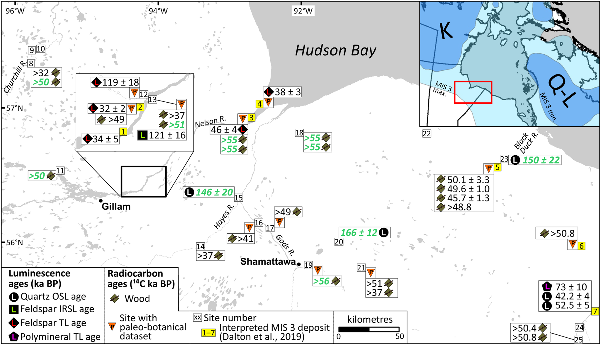
Figure 1. Geochronological data for Quaternary intertill nonglacial deposits in the western Hudson Bay Lowland region of central Canada. New ages from this study are green, bolded, and italicized. Sites 1–7 were interpreted as possible Marine Isotope Stage (MIS) 3-aged deposits (Dalton et al., Reference Dalton, Finkelstein, Forman, Barnett, Pico and Mitrovica2019), and readers are referred to the Supplementary Material 1 for additional details about site-specific geochronological data and references. Some sites are shown without data, due to vetting of potentially unreliable radiocarbon ages. The inset map shows the location of the study area in central Canada, relative to deglacial position of the Keewatin (K) and Quebec-Labrador (Q-L) Domes of the Laurentide Ice Sheet (LIS) and the Batchelor et al. (Reference Batchelor, Margold, Murton, Dalton, Gibbard, Stokes, Murton and Manica2019) minimum and maximum reconstruction limits for the LIS during MIS 3 at 45 ka. IRSL, infrared-stimulated luminescence; OSL, optically stimulated luminescence; TL, thermoluminescence.
The western HBL is a key region in the heart of the LIS, with an extensive pre-LGM stratigraphic record (Nielsen et al., Reference Nielsen, Morgan, Morgan, Mott, Rutter and Causse1986; Dredge et al., Reference Dredge, Morgan and Nielsen1990; Dalton et al., Reference Dalton, Finkelstein, Barnett, Väliranta and Forman2018). The stratigraphic record is fragmented (Gauthier et al., Reference Gauthier, Hodder, Ross, Kelley, Rochester and McCausland2019) and contains organic-bearing sediment deposited during at least two different ice-free interstadials and/or interglacial periods (Nielsen et al., Reference Nielsen, Morgan, Morgan, Mott, Rutter and Causse1986; Dredge and McMartin, Reference Dredge and McMartin2011). As such, detailed stratigraphic studies are necessary to identify the youngest intertill nonglacial sorted sediment bed(s) in the region. Following extensive stratigraphic work in the western HBL (Gauthier et al. Reference Gauthier, Hodder, Ross, Kelley, Rochester and McCausland2019 and references therein, Reference Gauthier, Hodder, Lian, Finkelstein, Dalton and Paulen2021, Reference Gauthier, Hodder and Ross2022; Hodder and Gauthier, Reference Hodder and Gauthier2019, Reference Hodder and Gauthier2021), we document a series of new ages, from both optical and radiocarbon dating methods, on the uppermost intertill organic-bearing and sorted sediments in the western HBL. We show that key stratigraphic beds, including some that were previously assigned to MIS 3, can now be more confidently assigned to MIS 5e.
METHODS
Field data
Sediment exposures investigated were first cleared of slumped detritus, exposing a continuous section with no gap, and then described in detail. This includes describing the grain size, structure, colour, thickness, lateral variations, composition (clast lithology and geochemistry), and ice-flow data of identified stratigraphic beds. Ice-flow data were obtained from studied sections by measuring the long-axis orientations, or fabric, of clasts within till. Elongate clasts, defined by a minimum 1.5 ratio of the a-axis (longest) to the b-axis (middle), will, in most cases, rotate within the till matrix and orient parallel to the direction of shear that the overriding glacier exerts on the till (Holmes, Reference Holmes1941; Hicock et al., Reference Hicock, Goff, Lian and Little1996). A minimum of 30 elongated clasts were measured at each of the nine clast-fabric sites, and the data set is provided in Supplementary Material 2.
This work highlights three new sites where the stratigraphically youngest intertill nonglacial bed was identified through regional mapping and the sediment was suitable for optical dating (Fig. 1, sites 15, 20, and 23). It also includes revision of two known sites, with the support of new stratigraphic correlations and radiocarbon ages from wood, where nonglacial beds were previously assigned to MIS 3 (Fig. 1, sites 3 and 4).
Optical dating
At sites 15, 20, and 23 (Fig. 1), the stratigraphically youngest intertill sorted sediments were sampled for optical age determination. Optical dating samples were collected by inserting opaque plastic tubes (~20 cm long and 5 cm in diameter) into the sediment faces, extracting them, and then sealing each end to preserve water content. Sample tubes were opened under appropriate laboratory lighting, and the light-exposed material at the ends of the tubes was removed and discarded. Bulk sediment extracted from the middle of the tubes was treated with HCl acid to remove any carbonates, and then by concentrated H2O2 to remove any disseminated organic matter. Sediment in the 180–250-μm-diameter size range was then extracted by wet sieving, and the quartz fraction was separated by density separation in lithium metatungstate. Quartz grains were then etched with concentrated HF acid to remove the outer alpha affected surfaces of the grains and to dissolve any remaining feldspar (e.g., Wintle, Reference Wintle1997). Aliquots consisted of 50–100 quartz grains mounted on aluminum disks using silicon oil as an adhesive.
Equivalent dose (D e) values were found using the single-aliquot regenerative-dose (SAR) method (Murray and Wintle Reference Murray and Wintle2000, Reference Murray and Wintle2003). Irradiations and luminescence measurements were made using a Risø TL/OSL DA-20 reader. Laboratory irradiations were applied using a calibrated 90Sr/90Y beta-source on the reader that delivered ~4.7 Gy/min to the sample grains. Aliquots were stimulated by exposing them to 56 mW/cm2 of blue (470 ± 20 nm) light for 100 s while being held at 125°C (Murray and Wintle, Reference Murray and Wintle2003). Ultraviolet emissions (~350 nm) were detected by an Electron Tubes Ltd. 9235QB photomultiplier tube placed behind a 7.5-mm-thick Hoya U-340 optical filter. An infrared “wash” (exposure to ~130 mW/cm2 of 870 ± 40 nm light for 100 s while at 50°C) was administered before stimulation with blue light to reduce or eliminate the signal from any contaminating feldspar (Olley et al., Reference Olley, Pietsch and Roberts2004; Wintle and Murray, Reference Wintle and Murray2006). Aliquots were accepted for SAR analysis if their natural signals showed a clear “fast” component. Dose–response data were generated by giving the aliquots various laboratory doses, up to ~400 Gy, and one of the doses was repeated to test the effectiveness of the chosen test dose to correct for sensitivity change incurred during the SAR cycles. A preheat temperature and duration of 220°C for 10 s was chosen, which is about midway in the range of typical values (160–300°C; Wintle and Murray, Reference Wintle and Murray2006) used by most practitioners for quartz. The preheat treatment administered after the test dose involved heating the aliquot to 160°C at a rate of 5°C/s and then turning off the heat. A “zero-dose” measurement was also included to measure the degree of thermal transfer (recuperation). For each aliquot, the luminescence measured over the last 20 s of 100 s of stimulation was subtracted from that recorded over the first 0.4 s of stimulation, and this was divided by that measured after the test dose. These data were plotted as a function of laboratory dose and were best fit with saturating exponential+linear curves. The luminescence intensity measured from a preheated aliquot of prepared grains that had received no laboratory dose (the “natural”) was interpolated onto its dose–response curve, and a D e value was measured from the dose axis; a representative example is show in Figure 2. Standard SAR quality control tests were applied, and these included assuring that the intensities of the recuperation signals were less than 5% of those of the natural signals and that recycling ratios were no more than ±10% of unity (Wintle and Murray Reference Wintle and Murray2006). Finally, the efficacy of the chosen SAR protocol was tested for each sample by means of dose-recovery tests (Wintle and Murray, Reference Wintle and Murray2006). For these, 15 aliquots were bleached by natural sunlight for 30 min, then given a laboratory dose approximately equal to the samples’ D e, and then the same SAR protocol was applied to see if that dose could be recovered.

Figure 2. Luminescence decay curve (main graph) showing the “natural” signal and a dose–response curve (inset) for sample 112-19-605-OSL-004. These curves are typical for the three samples analyzed in this study. Note that the initial part of the luminescence decay is dominated by the desired “fast” signal component. In each case, the final 20 s of the signal was subtracted from the initial 0.4 s, and this value (Li) was divided by that measured from a subsequent test dose (Ti) to produce the normalized (i.e., sensitivity-corrected) signal, which is plotted on the vertical axis of the dose–response curve graph. Note that the dose response is best fit by an exponential+linear function. The equivalent dose (D e) is estimated by interpolation of the natural signal onto the dose–response curve as shown.
Environmental dose rates (Table 1) were determined by drying and milling a representative fraction of the bulk sediment used for dating and analyzing for U, Th, and K by neutron activation analysis (Table 1). As all our samples consisted of well-drained sand, the as-collected water content was used in the dose-rate calculations, with a ±10% uncertainty (1σ) that is intended to account for moisture fluctuation over time. Dose rates were calculated using standard formulae (Aitken, Reference Aitken1985; Berger, Reference Berger and Easterbrook1988; Lian et al., Reference Lian, Hu, Huntley and Hicock1995) and the dose-rate scaling and conversion factors of Guérin et al. (Reference Guérin, Mercier and Adamiec2011) and Brennan (Reference Brennan2003), respectively. The contribution from cosmic ray radiation (Table 1) was estimated using present burial depths and the relationship of Prescott and Hutton (Reference Prescott and Hutton1994).
Table 1. Optical age sample water content, radioisotope concentrations, sample depths, and calculated dose rates.

a Δw = water content (mass water/mass dry sediment). For the dose-rate calculations, each Δw value included an uncertainty of ±10% (1σ) to account for fluctuations in water content over time.
b d = sample depth beneath the ground surface.
c Ḋ C = cosmic ray dose rate; Ḋ T = total dose rate (that due to cosmic rays plus that due to β and γ radiation).
Radiocarbon dating
Radiocarbon ages determined by accelerator mass spectrometry (AMS) were obtained from detrital wood (n = 8) and carbonate shell material (n = 5). Wood specimens were physically pretreated before analysis at the A.E. Lalonde AMS Laboratory or Keck Carbon Cycle AMS Laboratory at the University of California by removing the outer layer of the specimen and then chemically pretreated with an acid–alkali–acid wash. Carbonate shell specimens were physically pretreated before analysis at the A.E. Lalonde AMS Laboratory by removing porous or recrystallized areas with a Dremel bit and then chemically pretreated by etching with 0.2 N HCl to remove the outer 20–30% (Crann et al., Reference Crann, Murseli, St-Jean, Zhao, Clark and Kieser2017). Radiocarbon ages are interpreted as minimum limiting ages for the stratigraphic beds from which they were sampled.
Vetting of radiocarbon ages
Given the geochronological inconsistencies in the western HBL, we first vetted all new and previous radiocarbon ages for intertill sediments across the study area (Fig. 1, Supplementary Material 1), building upon Dalton et al. (Reference Dalton, Finkelstein, Forman, Barnett, Pico and Mitrovica2019). This vetting needs to be completed before interpretation to remove unreliable ages. Wood is the best material to attempt radiocarbon age determination when the material is near the upper limit of this geochronometer (e.g., Dalton et al., Reference Dalton, Finkelstein, Barnett and Forman2016; Bayliss and Marshall, Reference Bayliss and Marshall2019), and all vetted radiocarbon constraints for the western HBL are from wood (Fig. 1). Like others (e.g., Young et al. Reference Young, Reyes and Froese2021), we removed all ages from bulk organic samples (n = 6), because this material can more easily be contaminated by inclusion of older carbon (old detrital fragments) and/or by younger carbon (modern-day rootlets). For example, site 6 (Fig. 1) was included as a potential MIS 3 site in Dalton et al. (Reference Dalton, Finkelstein, Forman, Barnett, Pico and Mitrovica2019) based on an untreated bulk organic age of 37 ± 1.6 14C ka BP (WAT-1378). Yet there are another four nonfinite ages from pretreated bulk organics collected during this initial study and a nonfinite AMS age from wood (>50.8 14C ka BP, ISGS A1658) at the same site (Supplementary Material 1). Given that only one of the six ages is finite, and the source material is the least reliable of the group, this site should not be used to support MIS 3 deglaciation. We also removed the finite shell ages that are >40 ka (n = 4), because shell material is susceptible to some isotopic exchange with the surrounding environment (e.g., Ramsey, Reference Ramsey2008). This issue is not always minimized with physical and acid-etching pretreatment (method used in this study), and more advanced pretreatment procedures are necessary to gain confidence in shell radiocarbon ages (e.g., Douka et al., Reference Douka, Hedges and Higham2010).
RESULTS
Assessing the geochronological constraints
Ideally, multiple lines of geochronological evidence should be used to support any MIS 3 (considered to span ~57–29 ka) age determination without dispute. The vetted compilation of new and existing radiocarbon ages on sub-till wood shows only 1 out of 14 sites has finite radiocarbon ages; that one site also contains wood with a nonfinite radiocarbon age, indicating that these sediments are potentially older than MIS 3 (Fig. 1, site 5, Supplementary Material 1). Sediments with MIS 3 TL ages at sites 2 and 3 also contained wood with conflicting nonfinite radiocarbon ages (Fig. 1, Supplementary Material 1). Finding nonfinite radiocarbon age wood at two different sites decreases the likelihood of “transported” wood (i.e., reworked older wood). As pointed out by Roy (Reference Roy1998), the TL ages at sites 1–4 are likely underestimations due to the now better understood effect of anomalous fading on the luminescence signal of feldspars. Berger and Nielsen (Reference Berger and Nielsen1991) used long-term storage of their laboratory irradiated samples, some at an elevated temperature, in an attempt to reduce the effect of anomalous fading of the TL signal, but it has been found that this treatment is, at least for some samples, not sufficient (cf. Spooner Reference Spooner1992, Reference Spooner1993). Roy (Reference Roy1998) also questions these TL ages on the basis of the range of glow curve temperatures from which the TL signal used to build dose–response curves was determined and notes that inclusion of the “unstable” 270°C TL peak could have resulted in the calculated TL age being too young. This might be the case, as others have found that the infrared-stimulated luminescence (IRSL) signal associated with the 270°C TL peak is thermally unstable but are not certain that this is also the case for the TL signal from this peak (Duller and Bøtter-Jensen, Reference Duller and Bøtter-Jensen1993). Another point of concern are the dose rates reported by Berger and Nielsen (Reference Berger and Nielsen1991) for their samples, which are up to a factor of two higher than those reported by Roy (Reference Roy1998) for sediments extracted from the same stratigraphic bed. Indeed, one of our samples (not part of this study) collected from the same stratigraphic bed as the apparent MIS 3 age of Berger and Nielsen (Reference Berger and Nielsen1991) has radioisotope concentrations close to those of Roy (Reference Roy1998). These values are much lower than those presented in Berger and Nielsen (Reference Berger and Nielsen1991). If a dose rate that is the average of those of Roy (Reference Roy1998) is applied to the equivalent dose values of Berger and Nielsen (Reference Berger and Nielsen1991), the ages will almost double, and they would increase even more if corrected for anomalous fading. For these reasons, we believe that the previously reported TL ages of Berger and Nielsen (Reference Berger and Nielsen1991) are likely to be underestimations of the true depositional age, and we suggest that the ages should be removed from the MIS 3 age data set.
New optical ages
Three samples were collected for optical age determination (Fig. 1, sites 15, 20, and 23). For each sample, all the aliquots passed the SAR quality-control tests, but for some (5 to 10 aliquots per sample) their natural signals plotted beyond the last data point of their respective dose–response curves, and these were excluded from further analysis. The D e values from accepted aliquots were plotted on radial plots (Galbraith, Reference Galbraith2010; Fig. 3), and overdispersion (OD) values were calculated (Table 2). Overdispersion is the variation between individual aliquot D e values above and beyond that associated with analytical uncertainties. It has been demonstrated that for samples consisting of quartz grains that were mostly likely fully bleached, OD values from small multigrain aliquots (fewer than 100 grains per aliquot) are, on average, about 20% (Galbraith et al., Reference Galbraith, Roberts, Laslett, Yoshida and Olley1999; Lian and Roberts, Reference Lian and Roberts2006; Jacobs and Roberts, Reference Jacobs and Roberts2007), although for some of these samples, OD values are higher than 30% (Arnold and Roberts, Reference Arnold and Roberts2009). The convention therefore has been to use a weighted mean D e found using the central age model (CAM) (Galbraith et al., Reference Galbraith, Roberts, Laslett, Yoshida and Olley1999) for the age calculation for samples for which OD is 20% or less (Jacobs and Roberts, Reference Jacobs and Roberts2007). For samples with OD values higher than 20%, which are assumed to consist of grains that have been heterogeneously bleached before deposition, the minimum age model (MAM) is appropriate. In that case the MAM D e would give an approximation of true depositional age of a sample if a significant number of grains had been fully bleached, or it would give an age closer to the true age than that derived using the CAM if this is not the case. Experiments have shown that for some samples, OD measured from D e values derived from large aliquots (~80 grains) is less than that derived from small aliquots (<10 grains), and much less than that derived from aliquots that contain single grains (Galbraith et al., Reference Galbraith, Roberts and Yoshida2005; Arnold and Roberts, Reference Arnold and Roberts2009). These variations are likely due to averaging of various single-grain signals in multigrain aliquots. These observations, together with the fact that the sedimentology at our sample sites indicates that heterogeneous bleaching was highly probable before deposition and burial, suggest that the variation in D e values of the individual grains in our samples could be higher that that suggested by our multigrain OD values. As such, we have provided ages using both CAM and MAM (Table 2), but we suggest that the MAM ages should be used for our stratigraphic interpretations due to the nature of the depositional environments. The ages derived using the MAM are 146 ± 20 ka (site 15, sample 112-19-629-024), 166 ± 12 ka (site 20, sample 112-16-407-019), and 150 ± 22 ka (site 23, sample 112-19-605-004). Results of the dose-recovery experiments (Table 2) suggest that the chosen SAR protocol was sufficient for producing accurate D e and age values. In consideration of the inferred depositional environments for the units from which our optical dating samples were collected, these MAM ages should be considered to be upper limits. But because all three ages are statistically consistent (within 1σ of each other), the true age probably lies somewhere within the range indicated by their analytical uncertainties.

Figure 3. Radial plots (Galbraith Reference Galbraith2010) showing the distribution of equivalent dose (D e) values for each sample and estimations of representative D e values (weighted mean) used for dating, using either the central age model (CAM) or the minimum age model (MAM; solid line that intersects the curved axis). Values that plot in the shaded zones fall within 2σ of the weighted mean value.
Table 2. Number of aliquots measured, overdispersion values (OD), equivalent dose values (D e), optical ages, and dose-recovery (DR) ratios.

Note: OD and D e values calculated using the software of Liang and Forman (Reference Liang and Forman2019).
a N = number of aliquots accepted/number of aliquots measured.
b C determined using the central age model (CAM).
c M determined using the three-parameter minimum age model (MAM).
dDR = dose-recovery ratio (given dose/recovered dose).
Stratigraphy and age constraints
We highlight herein three sections that contain sediment suitable for optical dating and that our till-stratigraphic framework has identified as lying directly under an advance-phase till from the last glaciation. Two other sections then show the impact till stratigraphy can have on understanding the relative age of intertill nonglacial sediments.
Site 15
The exposed stratigraphy at site 15 consists of five beds (Fig. 4). The youngest, uppermost bed (Bed A) consists of horizontally bedded sand and gravel with minor clay (Fig. 4). Shell fragments were observed throughout the upper sediments and paired whole valves of Hiatella arctica occur between 4 and 5 m depths, indicative of deposition within a marine environment. The horizontal bedding and grain-size variations in Bed A are interpreted to represent postglacial marine transgression at this site. A 7.8-m-thick layer of brown, massive, matrix-supported diamicton (Fig. 4, Bed B) sharply underlies Bed A. The diamicton contains 10–15% clasts and has a sandy-silt matrix (27% sand, 56% silt, and 13% clay). The diamicton has a crumbly appearance with minor oxidation rind developed on joint surfaces. A 0.6-m-thick layer of matrix-supported, massive, sandy gravel (Bed C) sharply underlies Bed B. The gravel is poorly sorted and contains 40% clasts that are granule- to large pebble-sized. The lower 0.2 m of this gravel contains rip-up clasts of diamicton. This gravel is interpreted as a glaciofluvial or fluvial deposit based on the poorly sorted nature of the sediments. A 1.6-m-thick layer of well-sorted sand sharply underlies the gravel (Bed D). The sand is horizontally bedded, with bedding defined by textural differences between alternating beds of very fine sand and beds of medium- to coarse-grained sand (Bed D). Shell fragments were observed in the upper 0.1 m of the bedded sands. The sands were likely deposited in a shallow-marine environment, based on the rhythmic bedding, the low elevation (41 m asl), the position beneath postglacial Tyrrell Sea sediments, and the proximity to the modern shoreline (~90 km). More than 6.0 m of dark greyish-brown, massive, matrix-supported diamicton (Fig. 4, Bed E) sharply underlies Bed D sand. The diamicton contains 15% clasts and has a clayey sandy-silt matrix (25% sand, 54% silt, and 21% clay). The diamicton has a blocky appearance with oxidation rind on the joint surfaces and is relatively denser compared with the upper diamicton (Fig. 4). The massive structure, texture, typical glacigenic shape of the clasts (bullet-shaped, faceted, and striated), the modality and strength of the pebble fabric, and lateral continuity indicate that Bed B and E diamicton is subglacial traction till (Evans et al., Reference Evans, Phillip, Hiemstra and Auton2006). The stratigraphy at site 15 is interpreted to consist of postglacial marine sediments that are underlain by two till beds separated by intertill sorted sediments. The interpretation of a marine depositional environment for Bed D requires that Hudson Bay was ice-free and that relative sea level was higher than the present day. The age of the bedded, well-sorted sand (Bed D) was determined to be 146 ± 20 ka (Figs. 3 and 4, Table 2).

Figure 4. Quaternary stratigraphy and sediment photos of site 15. Till fabric data are plotted on equal area, lower hemisphere projection stereonets, with the principal eigenvalue (S1) and eigenvector (V1) values provided. Contours were generated using the Kamb method (Vollmer Reference Vollmer1995). The sample location for optical age determination is shown by the black circle with an “L.”
Site 20
The exposed stratigraphy at site 20 consists of four beds (Fig. 5). The uppermost stratigraphic bed (Bed A) consists of 1.0 m of massive, moderately to well-sorted sand that is interpreted to have been deposited in a postglacial subaqueous environment, which was likely Lake Agassiz, as this site is above the local Holocene marine limit (~145 m asl; Gauthier et al., Reference Gauthier, Kelley and Hodder2020) and the region was inundated by Lake Agassiz following deglaciation. Bed A sharply overlies 9.0 m of dark yellowish-brown, massive, matrix-supported diamicton (Bed B). The diamicton contains 10% clasts and has a sandy clayey-silt matrix (21% sand, 51% silt, and 28% clay). Bed B is in sharp contact with 1.4 m of grey, massive, matrix-supported diamicton that contains rip-up mud clasts (Bed C). The diamicton contains 10% clasts and has a silty-clay matrix (5% sand, 35% silt, and 60% clay). The massive structure, texture, and glacigenic shape of the clasts (bullet-shaped, faceted, and striated), the modality and strength of the pebble fabric, and lateral continuity indicate that Bed B and C diamicton is subglacial traction till (Evans et al., Reference Evans, Phillip, Hiemstra and Auton2006). Considering the fine-grained texture of Bed C and mud rip-up clasts, it is interpreted that the ice that deposited this bed likely advanced over fine-grained sediments. Tills B and C were likely deposited during the same ice-flow event, based on the similar ice-flow direction interpreted from till fabrics (Fig. 5). Underlying these two tills is 3.8+ m of well-sorted sand (Bed D). Within the upper 1.0 m of this bed, there is convolute bedding and dewatering structures at places laterally along the contact (Fig. 5). These structures could have formed syndepositional in a subaqueous environment or from postdepositional dewatering. Beyond 1.0 m depth into this bed, the sand is cross-bedded to ripple cross-laminated sand. This thick sequence of cross-bedded sands indicates unidirectional bedload transport within a low-flow regime. No evidence was observed for settling from a suspension cloud. The stratigraphy at site 20 is interpreted to consist of well-sorted, cross-bedded sand deposited during a nonglacial period that is overlain by glacial and postglacial sediments. The optical age of the rippled sands (Bed D) was determined to be 166 ± 12 ka (Figs. 3 and 5, Table 2). This optical age had a low overdispersion (15 ± 3%) and a unimodal aliquot D e population, which supports that the quartz grains were likely well bleached before burial. However, it is nevertheless possible that more than one age population exists and is masked, as our aliquots consist of 50–100 grains.

Figure 5. Quaternary stratigraphy and sediment photos of site 20. Till fabric data are plotted on equal area, lower hemisphere projection stereonets, with the principal eigenvalue (S1) and eigenvector (V1) values provided. Contours were generated using the Kamb method (Vollmer Reference Vollmer1995). The sample location for optical age determination is shown by the black circle with an “L.”
Site 23
The exposed stratigraphy at site 23 consists of four beds (Fig. 6). The youngest, uppermost bed (Bed A) consists of 1.5 m of horizontally bedded sand and gravel. Bed A is interpreted to have been deposited in a postglacial marine environment based on the sediment texture and regional setting, as this site is situated below the local Holocene marine limit (~145 m asl; Gauthier et al., Reference Gauthier, Kelley and Hodder2020) and the top of the section is 26 m above the modern sea-level elevation. Bed A sharply overlies 1.4 m of brown to dark greyish-brown, massive, matrix-supported diamicton (Bed B). The diamicton contains 5% clasts and has a sandy clayey-silt matrix (24% sand, 51% silt, and 25% clay). The diamicton has a minor blocky structure with oxidation rind on the joint surfaces. This diamicton, like the others described at sites 15 and 20, has all the main characteristics of a subglacial traction till. Bed B sharply overlies massive silt and massive to horizontally bedded fine sand to silty fine sand that contains disseminated organic material (Bed C). The presence of organic material requires terrestrial input into the depositional environment. Thus, the sediments that were targeted for optical dating were likely transported within a fluvial environment before deposition, which should be favourable to sufficient light exposure before burial. Bed C sharply overlies 3.3+ m of poorly sorted, matrix-supported sandy gravel (Bed D). Bed D gravel contains granule- to small cobble-sized clasts and rare shell fragments and is interpreted to have been deposited in a subaqueous environment. The subtill sediments (Beds C and D) indicate an overall fining upward sequence, possibly deposited in a fluvial environment. The stratigraphy at site 23 is interpreted to consist of nonglacial sediments that are overlain by glacial and postglacial sediments. The optical age of the organic-bearing fine sand (Bed C) was determined to be 150 ± 22 ka (Figs. 3 and 6, Table 2).

Figure 6. Quaternary stratigraphy and sediment photos of site 23. Till fabric data are plotted on equal area, lower hemisphere projection stereonets, with the principal eigenvalue (S1) and eigenvector (V1) values provided. Contours were generated using the Kamb method (Vollmer Reference Vollmer1995). The sample location for optical age determination is shown by the black circle with an “L.”
Till stratigraphy as an important tool
Sites 3 and 4 (Fig. 7) are located ~10–12 km apart, and the stratigraphy at both sites was previously interpreted to contain one correlative intertill nonglacial bed (Dredge and Nielsen, Reference Dredge and Nielsen1985; Dredge et al., Reference Dredge, Morgan and Nielsen1990; Dredge and McMartin, Reference Dredge and McMartin2011). At site 3, the Bed C gravel is discontinuous across the exposure and pinches out to a till–till contact between Beds B and D in places. Bed C gravel contains an in situ peat bed with large (>10 cm) wood fragments that yielded a nonfinite radiocarbon age (>55 14C ka BP, UOC-10974). Similarly, a detrital wood fragment from the gravel underlying the peat bed yielded a nonfinite radiocarbon age (>55 14C ka BP, UOC-10975). Paleobotanic data from these sediments indicate a northern boreal forest to forest–tundra environment, similar to the present day for that area (Dredge et al., Reference Dredge, Morgan and Nielsen1990). Hence, these uppermost intertill nonglacial sediments are interpreted to have been deposited during the last interglacial period (MIS 5e; Dredge et al., Reference Dredge, Morgan and Nielsen1990), leading us to reject the MIS 3 TL age at site 3 (46 ± 4 ka; Berger and Nielsen, Reference Berger and Nielsen1991) when conditions must have been colder based on the global sea-level record (Lisiecki and Raymo, Reference Lisiecki and Raymo2005).

Figure 7. Quaternary stratigraphy at sites 3 and 4 in the on the Nelson River at Hudson Bay. The stratigraphic beds identified have been interpreted based on qualitative and quantitative observations. The thermoluminescence (TL) age estimations for stratigraphic beds (Berger and Nielsen, Reference Berger and Nielsen1991) are interpreted to be age underestimations.
Bed C is missing between beds B and D at site 4 (Fig. 7). However, site 4 does expose nonglacial sediments below Bed D that have a TL age of 38 ± 3 ka (Berger and Nielsen, Reference Berger and Nielsen1991; Fig. 1). Bed E consists of a clay-rich diamicton that contains whole valves of Macoma calcarea (Fig. 7), interpreted as a glaciomarine deposit. Underlying Bed E is massive, blue clay (Bed F-1), interpreted as a marine deposit. Owing to the principles of superposition and relative age, and perhaps ignoring the differences between till Beds B and D, Bed C at site 3 was originally correlated to Bed F-1 at site 4 (Dredge et al., Reference Dredge, Morgan and Nielsen1990; Dredge and McMartin, Reference Dredge and McMartin2011).
At site 3, we documented a newly discovered second, lower, intertill nonglacial bed, which indicates that there are actually two intertill nonglacial beds exposed in the stratigraphic record at site 3 (Fig. 7, Bed F-2). This lowermost intertill nonglacial bed consists of well-sorted, horizontally bedded sands (Bed F-2). To support correlations between sites 3 and 4, we examined the tills in addition to the sorted sediments. The upper till (Bed B) is significantly less dense, is sandier, and has a higher proportion of carbonate detritus compared with the middle till (Bed D), enabling stratigraphic correlation between these two sites (Supplementary Material 3). These differences, together with the knowledge that Bed C was deposited between the two tills, shows that the subtill marine sediments at site 4 are correlated to the second, older nonglacial unit at site 3 (Fig. 7, Bed F). Thus, while Bed C was deposited during MIS 5e, based on nonfinite radiocarbon ages, regional stratigraphy, and pollen data, the Bed F intertill sediments are even older (pre–MIS 5).
The reassessment of the stratigraphy at sites 3 and 4 indicates that the previously reported MIS 3 TL age from Bed F at site 4 (38 ± 3 ka), like the other TL ages in the region, is underestimated (Fig. 1). Furthermore, the stratigraphic evidence confirms that the near-finite radiocarbon age (49.9 ± 1.0 ka 14C yr BP, UOC-13465) from a Macoma calcarea whole valve in Bed E is not accurate and supports our approach of removing near-finite shell 14C ages from the data set. The stratigraphy here also highlights the importance of studying till beds, because the first bed of nonglacial sorted sediments encountered below till may not relate to the most recent ice-free period (i.e., site 4).
DISCUSSION
Optical dating
Doses of up to 400 Gy needed to be applied in the SAR sequences to be able to interpolate the natural quartz luminescence signals from a sufficient number of aliquots onto their dose–response curves. The high doses resolved a dose response that was best fit with a saturating exponential that includes a linear component (Fig. 2). An exponential+linear dose response has been observed for quartz in many other studies, but the reason for its existence and its efficacy for dating remains uncertain. Some workers have found that for samples expected to have ages >100 ka that exhibit exponential+linear dose responses, standard SAR protocols perform well and yield ages consistent with independent information (e.g., Murray et al., Reference Murray, Buylaert, Henriksen, Svendsen and Mangerud2008; Pawley et al., Reference Pawley, Bailey, Rose, Moorlock, Hamblin, Booth and Lee2008, Reference Pawley, Toms, Armitage and Rose2010), while there have been other studies that show that exponential+linear dose responses produce ages that are too young when compared with independent information (see review by Lowick and Preusser, Reference Lowick and Preusser2011). For many of these studies, however, reliable independent age information is lacking. A detailed study that examined the effectiveness of the SAR protocol for dating fine-grained quartz samples with exponential+linear dose responses has found that it performs well (e.g., Lowick and Preusser, Reference Lowick and Preusser2011); it is therefore possible that the usefulness of the exponential+linear signal in quartz for dating is sample dependent. Nonetheless, more work clearly needs to be undertaken to better understand the underlying physical processes; until that is done, ages found from samples with exponential+linear dose responses should be considered with some caution (e.g., Li et al., Reference Li, Roberts, Jacobs and Li2015).
This study targeted intertill sorted sediment beds that were identified using a regional till stratigraphic framework to have been deposited during the penultimate deglaciation of the region. At face value, two of our optical ages are within 1σ of MIS 5e, which is an expected ice-free period in the HBL considering this was a period of time with significantly reduced global ice volume (Lisiecki and Raymo, Reference Lisiecki and Raymo2005). The third age (166 ± 12 ka) is not within 1σ of MIS 5e, but based on the stratigraphy at this site, these sediments could have been deposited during the deglaciation phase of MIS 6. Furthermore, terrestrial glaciation is not always synchronous with marine isotope stages (Gibbard and Hughes, Reference Gibbard and Hughes2021), and it is therefore possible that the timing of glaciation in the HBL was slightly out of phase with the timing of climate shifts recorded in the marine record. It is likely that any overestimation of our optical ages is due to the inclusion of a sufficient number of grains whose signals were not adequately reset before burial.
K-feldspar is also routinely used for optical dating, and its upper age limit is usually higher than that for quartz but it was not used in this study, because its dose response was expected to be nonlinear in the region of our samples’ natural luminescence signals, and it therefore would not be possible to correct them for anomalous fading (Huntley and Lamothe, Reference Huntley and Lamothe2001). The post-IR IR (pIR-IR) signal from K-feldspar, which usually fades less (in some cases negligibly), was also not investigated, as its signal resets (bleaches) relatively slowly, and it was therefore anticipated that this would be a problem for the fluvial and lakeshore sedimentary environments sampled here. Another option for dating quartz in this region would be to investigate the thermally transferred optically stimulated luminescence (TT-OSL) signal, which has been observed to maintain a dose response defined by a single saturating exponential, even at high doses (e.g., Neudorf et al. Reference Neudorf, Lian, McIntosh, Gingerich and Augustinus2019), but like the pIR-IR signal from feldspar, the TT-OSL signal from quartz bleaches much more slowly than the standard quartz signal used for dating (Jacobs et al. Reference Jacobs, Meyer, Roberts, Aldeias, Dibble and El Hajraoui2011; Neudorf et al. Reference Neudorf, Lian, McIntosh, Gingerich and Augustinus2019), and it would therefore be expected to be of limited use for the sedimentary environments studied here; aeolian units would need to be identified. Dating aliquots that consist of single grains of quartz would be an advantage, as D e populations would be easier to identify using the MAM, or the finite mixture model, which is suited to analysis of D e values derived from single-grain aliquots, but can present serious problems when applied to multigrain aliquots (Arnold and Roberts Reference Arnold and Roberts2009). However, routine SAR dating of single grains from the samples studied here is not practical, as the sensitivity of the quartz in the region is variable, and would require thousands of grains being analyzed. Moreover, the depositional age of the samples requires high-dose irradiations and therefore exceedingly long machine time. Nevertheless, single-grain dating of a few key strata in the region, including some where reliable independent age information is available, should be considered in future research.
Resolving the age of the Black Duck River nonglacial sediments
The organic-bearing nonglacial sediments at site 5 (Fig. 1) are described to be near the surface and overlain by ~1.5 m of gravel that is interpreted to have been deposited in a postglacial marine environment (Dalton et al., Reference Dalton, Finkelstein, Barnett and Forman2016). Three of the four radiocarbon ages on wood from the organic-bearing nonglacial sediments are near-infinite (45.7 ± 1.3 14C ka BP, ISGS-A1656; 49.6 ± 1.0 14C ka BP, UOC-0587; 50.1 ± 3.3 14C ka BP, ISGS-A1995), which led to the interpretation that these sediments were deposited during MIS 3 (Dalton et al., Reference Dalton, Finkelstein, Barnett and Forman2016, Reference Dalton, Finkelstein, Forman, Barnett, Pico and Mitrovica2019). Dalton et al. (Reference Dalton, Finkelstein, Barnett and Forman2016) considered these ages reliable, based on the repeatability of the radiocarbon ages from different laboratories, and stratigraphic-age agreement. Importantly though, the paleobotanic data from the site 5 organic-bearing bed indicate a paleoenvironment dominated by boreal and peatland taxa, similar to vegetation currently present in the region (Dalton et al., Reference Dalton, Finkelstein, Hodder and Gauthier2022a). Quantitative paleoenvironmental reconstruction of these sediments indicates the mean summer temperature varied between 9.4 and 14.5°C compared with the present-day 11°C, and total precipitation was similar to the present-day precipitation (467 mm; Dalton et al., Reference Dalton, Finkelstein, Hodder and Gauthier2022a). This evidence of climatic conditions similar to those of the present day supports deposition during an interglacial period, such as MIS 5e, as it is difficult to reconcile a climate reconstruction similar to the present day with the LIS still covering large areas of North America in the most restrictive reconstructions for MIS 3 (e.g., Batchelor et al., Reference Batchelor, Margold, Murton, Dalton, Gibbard, Stokes, Murton and Manica2019; Gowan et al., Reference Gowan, Zhang, Khosravi, Rovere, Stocchi, Hughes, Gyllencreutz, Mangerud, Svendsen and Lohmann2021). As such, it seems likely that the nonfinite radiocarbon age is more reliable than those near-finite from the same strata, and that deposition at site 5 occurred during MIS 5e.
This study attempted to obtain an optical age from the nonglacial sediments at the Black Duck River site 5 to test the accuracy of the near-finite radiocarbon ages from wood; however, the exact site could not be accurately located in the field based on published location information. While the stratigraphy at site 23 on the Black Duck River (Fig. 6) in this study is different from site 5, considering that both of these sections contain near-surface interglacial deposits and are situated within ~1 km of each other, we interpret that the organic-bearing Bed C at site 23 is likely correlated to the organic-bearing nonglacial bed at site 5 studied by Dalton et al. (Reference Dalton, Finkelstein, Barnett and Forman2016). Owing to the susceptibility of near-infinite radiocarbon ages to modern contamination (e.g., Reyes et al., Reference Reyes, Dillman, Kennedy, Froese, Beaudoin and Paulen2020), the presence of one nonfinite radiocarbon age, and paleoenvironmental information consistent with a climate warmer than that expected during MIS 3, we consider our site 23 to have more reliable stratigraphy and chronological data than site 5 (Dalton et al., Reference Dalton, Finkelstein, Barnett and Forman2016). Thus, we suggest that the optical age at site 23 (150 ± 22 ka), within 1σ error of MIS 5e, more accurately dates the deposition of interglacial sediments situated on the Black Duck River and is in better agreement with pollen profile from this bed at site 5.
HBL evidence for MIS 3 deglaciation?
Vetting of previous radiocarbon ages, together with new optical and radiocarbon ages, has led to removal of sites 1–6 from the MIS 3 age data set in the western HBL (Fig. 1, inset). That leaves site 7, where two MIS 3 optical ages were obtained from quartz grains (42.2 ± 4 and 52.5 ± 5 ka; Dalton et al., Reference Dalton, Finkelstein, Barnett and Forman2016), as well as an older TL age of 73 ± 10 ka (Forman et al., Reference Forman, Wintle, Thorleifson and Wyatt1987) from subtill sediments interpreted to be marine. A third MIS 3 optical age provided in Dalton et al. (Reference Dalton, Finkelstein, Barnett and Forman2016) is from the Drowning River near James Bay (~540 km to the southeast of site 7). At this site, the quartz optical age of 42.9 ± 3.7 ka is incompatible at 1σ error with two nonfinite AMS radiocarbon ages on wood (>48.4 14C ka BP, ISGS 2463; >51.7 14C ka BP, ISGS |A2425; Dalton et al., Reference Dalton, Finkelstein, Barnett and Forman2016). The inconsistency between the optical ages and nonfinite radiocarbon ages at this site raises questions about the accuracy of the optical ages in Dalton et al. (Reference Dalton, Finkelstein, Barnett and Forman2016). Furthermore, Gao et al. (Reference Gao, Huot, McDonald, Crabtree and Turton2020) report new chronological data from a site just 16 km away from the Dalton et al. (Reference Dalton, Finkelstein, Barnett and Forman2016) Drowning River site, with an optical age from feldspar that is much older than MIS 3 (118 ± 13 ka); correlation of the two subtill units is unclear. The optical age provided by Gao et al. (Reference Gao, Huot, McDonald, Crabtree and Turton2020) is likely a lower limit, as an age of this magnitude is expected to have a dose response that is nonlinear, and such ages cannot be corrected for anomalous fading using the method of Huntley and Lamothe (Reference Huntley and Lamothe2001). However, Gao et al. (Reference Gao, Huot, McDonald, Crabtree and Turton2020) do not provide representative dose–response curves necessary to fully evaluate the efficacy of their fading correction procedure. As such, site 7 will require additional investigation to confirm the sediments there are indeed MIS 3. For now, it remains the only site with an MIS 3 age in western HBL, in contrast to the great number of sites with nonfinite radiocarbon ages or older optical ages (Fig. 1).
Our new minimum limiting radiocarbon and optical ages for the stratigraphically youngest intertill nonglacial sediments in the western HBL indicate that these sediments were likely deposited during MIS 5e to late MIS 6. Hence, we find there is insufficient stratigraphic and geochronological evidence for models and reconstructions (e.g., Carlson et al., Reference Carlson, Tarasov and Pico2018; Gowan et al., Reference Gowan, Zhang, Khosravi, Rovere, Stocchi, Hughes, Gyllencreutz, Mangerud, Svendsen and Lohmann2021) to consider the western HBL region ice-free during MIS 3. Additional work is needed to pinpoint the southern margin of the LIS in central Canada during this time period.
As pointed out by Miller and Andrews (Reference Miller and Andrews2019), the timing and provenance of large iceberg discharge events into the North Atlantic, which are recorded by Heinrich layers (e.g., Hemming, Reference Hemming2004), can provide an important proxy for ice extent and need to be reconciled with HBL age constraints. Heinrich events H4 (~38 ka) and H5 (~45 ka), which occurred during MIS 3, have a provenance signature similar to that of Heinrich event H2 (~24 ka), which has long been associated with the Hudson Strait Ice Stream, and a catchment zone extending deep into Hudson Bay and perhaps beyond (e.g., Hemming, Reference Hemming2004; Ross et al., Reference Ross, Lajeunesse and Kosar2011; Miller and Andrews, Reference Miller and Andrews2019). As pointed out by Roy et al. (Reference Roy, Hemming and Parent2009), some uncertainties persist about the exact provenance of the sediment, but an ice sheet over Hudson Bay during MIS 3 feeding a long, topographically controlled Hudson Strait Ice Stream remains the most plausible model for the source of Heinrich layers H4 and H5. Configuration of a “big” ice sheet is also in agreement with the interpretation that the Hudson Strait Ice Stream was stable at the ice shelf during H4 and H5 (Rashid et al., Reference Rashid, Piper, Drapeau, Marin and Smith2019). Heinrich events thus provide additional independent support for a glaciation of Hudson Bay and the western HBL during MIS 3.
CONCLUSIONS
New age determinations from the uppermost intertill nonglacial sediments, combined with consideration of the paleobotanic data sets in the western HBL stratigraphic record, suggest that the region was last deglaciated during MIS 5e. New radiocarbon ages and vetting of the radiocarbon age data set, together with the new optical ages and detailed stratigraphic correlations herein, have removed six sites from the HBL “MIS 3” data set, leaving just one potential MIS 3 site that has conflicting age assignments.
The Quaternary stratigraphy of the HBL is highly fragmented, which hampers correlations and also indicates that previous investigations of the region have provided an oversimplified stratigraphic framework. This complex stratigraphic record, including detailed lithostratigraphy of enclosing glacial units, needs to be considered alongside geochronology results to provide robust reconstructions of Late Quaternary nonglacial events. This study suggests that the LIS southern margin did not retreat north or northeast of the western HBL and that Hudson Bay remained glaciated during MIS 3. Future studies to determine the maximal or minimal extent of the LIS during MIS 3 should continue reconstruction of the stratigraphic record south of the western HBL.
Supplementary Material
The supplementary material for this article can be found at https://doi.org/10.1017/qua.2023.35
Acknowledgments
April Dalton is thanked for stimulating discussions regarding the HBL region and her continuous effort to characterize subtill nonglacial deposits. The Manitoba Geological Survey is thanked for field and analytical funding. We thank Vanessa Brewer and Nicola Ferguson (University of the Fraser Valley) for careful preparation and measurement of the optical dating samples. OBL acknowledges support from Natural Sciences and Engineering Research Council (NSERC) of Canada Discovery and Research Tools and Instrument grants. This article greatly benefited from reviews by the senior editor Nicholas Lancaster, associated editor Tom Lowell, Sarah Finkelstein, and one anonymous reviewer.


 Open access