


INTRODUCTION
Records from basins with restricted connection to the open ocean provide essential information about the effect of climate-driven processes on hydrographic systems. Sediment archives from such areas document environmental alternations as composite results of the effects of long- and short-term climatic changes, the fluctuations of sea level stands, and freshwater input in the basin (i.e., Baltic Sea: Sohlenius et al., Reference Sohlenius, Sternbeck, Andren and Westman1996; Black Sea-Marmara Sea complex: McHugh et al., Reference McHugh, Gurung, Giosan, Ryan, Mart, Sancar, Burckle and Çagatay2008; Hoyle et al., Reference Hoyle, Bista, Flecker, Krijgsman and Sangiorgi2021; Gulf of Corinth, Greece: McNeill et al., Reference McNeill, Shillington, Carter, Everest, Gawthorpe, Miller and Phillips2019). Within this context, the Red Sea is considered to be a prominent region for paleoclimatic and paleoceanographic studies (Rohling et al., Reference Rohling, Fenton, Jorissen, Bertrand, Ganssen and Caulet1998; Siddall et al., Reference Siddall, Smeed, Hemleben, Rohling, Schmelzer and Peltier2004).
The Red Sea is a narrow, semi-closed basin situated in an arid climate zone, and is connected at its southern end with the Indian Ocean via the 20-km-wide Bab el Mandeb Straits (Fig. 1a, b). On the basin-inward side of the straits lies the Hanish sill (137 m in depth), which, as the shallowest passage in the Red Sea connection with the Gulf of Aden (GoA), is critical in regulating water dynamics in the basin and controlling the exchange of water masses between the Red Sea and northwestern Arabian Sea (NWArS) (Rohling, Reference Rohling1994; Rohling et al., Reference Rohling, Fenton, Jorissen, Bertrand, Ganssen and Caulet1998; Siddall et al., Reference Siddall, Smeed, Matthiesen and Rohling2002; Biton et al., Reference Biton, Gildor and Peltier2008).
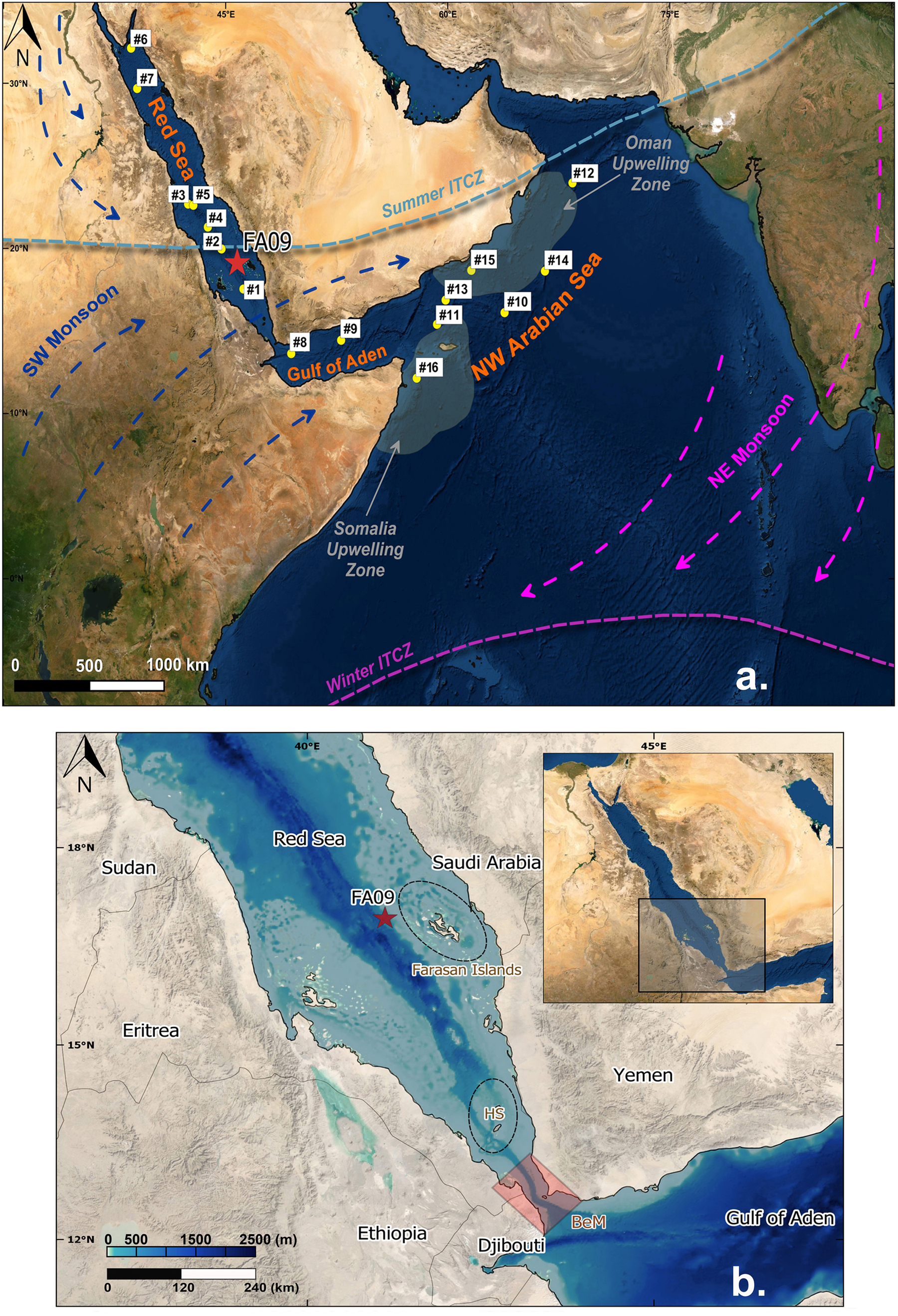
Figure 1 (a) The wider area of Red Sea, Gulf of Aden, and northwestern Arabian Sea, with the locations of the cores referred in the text (Table 1). (b) The southern Red Sea and location of FA09. The Farasan Islands archipelago and Hanish sill (HS) are indicated with elliptic shapes; the strait of Bab-el-Mandeb (BeM) is highlighted with the red rectangle.
Over Quaternary glacial-interglacial cycles, Red Sea environmental conditions have developed in accordance with sea level changes and the influence of Arabian Sea water masses driven by the South Asian Monsoon System (SAMS) (Locke and Thunell, Reference Locke and Thunell1988; Almogi-Labin et al., Reference Almogi-Labin, Hemleben, Meischner and Erlenkeuser1996; Hemleben et al., Reference Hemleben, Meischner, Zahn, Almogi-Labin, Erlenkeuser and Hiller1996; Rohling et al., Reference Rohling, Fenton, Jorissen, Bertrand, Ganssen and Caulet1998; Arz et al., Reference Arz, Pätzold and Müller2003b). At times of full glacial stages of the last 500 ka, the sea level lowstands limited the basin's connection with the Indian Ocean (Rohling et al., Reference Rohling, Fenton, Jorissen, Bertrand, Ganssen and Caulet1998; Siddall et al., Reference Siddall, Rohling, Almogi-Labin, Hemleben, Meischner, Schmeltzer and Smeed2003; Lambeck et al., Reference Lambeck, Purcell, Flemming, Vita-Finzi, Alsharekh and Bailey2011), leading to near-isolation of the basin, which caused hypersaline conditions in the central and northern parts (Locke and Thunnel, Reference Locke and Thunell1988; Hemleben et al., Reference Hemleben, Meischner, Zahn, Almogi-Labin, Erlenkeuser and Hiller1996; Fenton et al., Reference Fenton, Geiselhart, Rohling and Hemleben2000; Biton et al., Reference Biton, Gildor and Peltier2008).
The SAMS operates on orbital timescales, following the Milankovitch cycles band and solar insolation intensity (Clemens and Prell, Reference Clemens and Prell2003; Leuschner and Sirocko, Reference Leuschner and Sirocko2003; Kathayat et al., Reference Kathayat, Cheng, Sinha, Spötl, Edwards, Zhang and Li2016). On shorter, (multi)millennial timescales, a synchronicity has been observed between abrupt climate events in the North Atlantic and the SAMS domains, implying a climatic teleconnection between the two regions (Sirocko et al., Reference Sirocko, Gabre-Schonberg, McIntyre and Molfino1996; Schulz et al., Reference Schulz, Von Rad and Erlenkeuser1998; Leuschner and Sirocko, Reference Leuschner and Sirocko2000; Deplazes et al., Reference Deplazes, Lückge, Peterson, Timmermann, Hamann, Hughen and Röhl2013). Cool episodes in the North Atlantic, often associated with massive iceberg-discharge events and formation of ice-rafted debris (IRD) deposits (i.e., Heinrich stadials; Sanchez-Goni and Harrison, Reference Sanchez-Goni and Harrison2010), coincide with phases of southward migration of the Intertropical Convergence Zone (ITCZ), low levels of monsoonal precipitation, and dominant northeast monsoon (NEM) winds, leading to increased aridity in the Arabian Sea (Gupta et al., Reference Gupta, Anderson and Overpeck2003; Ivanochko et al., Reference Ivanochko, Ganeshram, Brummer, Ganssen, Jung, Moreton and Kroon2005; Singh et al., Reference Singh, Jung, Darling, Ganeshram, Ivanochko and Kroon2011; Deplazes et al., Reference Deplazes, Lückge, Stuut, Pätzold, Kuhlmann, Husson, Fant and Haug2014) and Red Sea (Arz et al., Reference Arz, Pätzold and Müller2003b; Legge et al., Reference Legge, Mutterlos and Arz2006; Rohling et al., Reference Rohling, Grant, Hemleben, Kucera, Roberts, Schmeltzer, Schulz, Siccha, Siddall and Trommer2008; Trommer et al., Reference Trommer, Siccha, Rohling, Grant, Meer, Van Der, Schouten, Hemleben and Kucera2010; Roberts et al., Reference Roberts, Rohling, Grant, Larrasoaña and Liu2011) areas. On the other hand, millennial-scale warm and humid phases in high latitudes correspond to phases of northward displacement of the ITCZ and intensified southwest monsoon (SWM) winds, leading to high precipitation levels in the tropics (Fleitmann et al., Reference Fleitmann, Burns, Mangini, Mudelsee, Kramers, Villa and Neff2007; Shakun et al., Reference Shakun, Burns, Fleitmann, Kramers, Matter and Al-Subary2007). The SWM triggered upwelling of subsurface, nutrient-rich, and relatively low-temperature/salinity waters in the NWArS around the Oman and Somalia margins (Fig. 1a) (Emeis et al., Reference Emeis, Anderson, Doose, Kroon and Schulz-Bull1995; Pourmand et al., Reference Pourmand, Marcantonio, Bianchi, Canuel and Waterson2007; Böll et al., Reference Böll, Schulz, Munz, Rixen, Gaye and Emeis2015; Gaye et al., Reference Gaye, Böll, Segschneider, Burdanowitz, Emeis, Ramaswamy, Lahajnar, Lückge and Rixen2018).
Previous studies have employed planktic foraminifera associations for reconstructing past monsoon dynamics in the Arabian Sea (Anderson and Prell, Reference Anderson and Prell1991; Naidu and Malmgren, Reference Naidu and Malmgren1996; Cayre et al., Reference Cayre, Beaufort and Vincent1999; Almogi-Labin et al., Reference Almogi-Labin, Schmiedl, Hemleben, Siman-tov, Segl and Meischner2000; Schulz et al., Reference Schulz, Von Rad, Ittekkot, Clift, Kroon, Gaedicke and Craig2002; Ivanova et al., Reference Ivanova, Schiebel, Deo, Schmiedl, Niebler and Hemleben2003; Ishikawa and Oda, Reference Ishikawa and Oda2007; Caley et al., Reference Caley, Malaizé, Zaragosi, Rossignol, Bourget, Eynaud, Martinez, Giraudeau, Charlier and Ellouz-Zimmermann2011; Singh et al., Reference Singh, Jung, Darling, Ganeshram, Ivanochko and Kroon2011, Reference Singh, Tiwari, Shrivastava and Sinha2016). A key observation of these studies is the increased abundance of Globigerina bulloides (followed by Globigerinita glutinata and neogloboquadrinids), indicating increased upwelling and elevated productivity levels likely caused by enhanced SWM. Moreover, these elevated productivity levels were accompanied by notable reductions in the δ18O and δ13C records, which are interpreted as the result of intense water mixing and/or SST perturbations driven by strong SWM winds (Sirocko et al., Reference Sirocko, Sarnthein and Erlenkeuser1993; Naidu, Reference Naidu2004; Saher et al., Reference Saher, Jung, Elderfield, Greaves and Kroon2007; Ganssen et al., Reference Ganssen, Peeters, Metcalfe, Anand, Jung, Kroon and Brummer2011). This faunal and isotopic pattern is observed today in the upwelling regions of the Arabian Sea during the SWM season (Kroon and Ganssen, Reference Kroon and Ganssen1989; Conan and Brummer, Reference Conan and Brummer2000; Peeters et al., Reference Peeters, Brummer and Ganssen2002; Schiebel et al., Reference Schiebel, Zeltner, Treppke, Waniek, Rixen and Hemleben2004).
The large majority of the investigated Red Sea records are distributed in the central and northern sectors of the basin (Reiss et al., Reference Reiss, Luz, Almogi-Labin, Halicz, Winter and Wolf1980; Almogi-Labin et al., Reference Almogi-Labin, Hemleben, Meischner and Erlenkeuser1991, Reference Almogi-Labin, Hemleben, Meischner and Erlenkeuser1996; Hemleben et al., Reference Hemleben, Meischner, Zahn, Almogi-Labin, Erlenkeuser and Hiller1996; Rohling et al., Reference Rohling, Fenton, Jorissen, Bertrand, Ganssen and Caulet1998; Arz et al., Reference Arz, Lamy, Pätzold, Müller and Prins2003a, Reference Arz, Pätzold and Müllerb, Reference Arz, Lamy and Pätzold2006; Legge et al., Reference Legge, Mutterlos and Arz2006; Edelman-Furstenberg et al., Reference Edelman-Furstenberg, Almogi-Labin and Hemleben2009; Siccha et al., Reference Siccha, Trommer, Schulz, Hemleben and Kucera2009; Trommer et al., Reference Trommer, Siccha, Rohling, Grant, Meer, Van Der, Schouten, Hemleben and Kucera2010, Reference Trommer, Siccha, Rohling, Grant, Meer, Van Der, Schouten, Baranowski and Kucera2011; Hartman et al., Reference Hartman, Torfstein and Almogi-Labin2020). However, sea level and monsoon effects are pronounced in the southern sector due to its close proximity to the adjacent Arabian Sea (Locke and Thunell, Reference Locke and Thunell1988; Fenton et al., Reference Fenton, Geiselhart, Rohling and Hemleben2000; Badawi, Reference Badawi2015). The present study focuses on sediment core FA09 from the Farasan Archipelago (16.93°N, 41.12°E, 302 m water depth) retrieved from the deep outer part of the southern Red Sea continental shelf (Fig. 1b) during the DISPERSE project (Bailey et al., Reference Bailey, Deves, Inglis, Meredith-Williams, Momber, Sakellariou, Sinclair, Rousakis, Ghamdi and Alsharekh2015). Geraga et al. (Reference Geraga, Sergiou, Sakellariou, Rohling, Rasul and Stewart2019) presented initial micropaleontological results for the upper half of the core. Here, we present high-resolution micropaleontological (planktic foraminifera), stable isotope (δ18Ο, δ13C), and transfer-function (Artificial Neural Networks) analyses of paleo-sea surface temperature (SST) and salinity (SSS) on the entire core, spanning the last 30 ka. Our results are integrated with other records from the surrounding area (Fig. 1a, Table 1) to evaluate the regional paleoceanographic evolution. We thus advance our understanding of the spatial variation of Red Sea oceanographic changes over time, and specifically highlight interactions between the southern section and the NWArS since the late Marine Isotope Stage 3.
Table 1. Sediment cores from the wider area (Fig. 1a) used for comparisons in the present study.

OCEANOGRAPHIC BACKGROUND
Today, the Red Sea is characterized by arid, subtropical conditions (see Table 2 for data) and is one of the warmest and saltiest marine basins in the world (Sofianos and Johns, Reference Sofianos and Johns2007; Chaidez et al., Reference Chaidez, Dreano, Agusti, Duarte and Hoteit2017). The basin's hydrography is largely controlled by the seasonal variations of the SAMS. The SAMS is defined by seasonal movement of the winter-hemisphere Hadley cells across the equator, which also controls the latitudinal position of the Intertropical Convergence Zone (ITCZ) and the extent of the monsoonal rainbelt (Donohoe et al., Reference Donohoe, Marshall, Ferreira and Mcgee2013; McGee et al., Reference McGee, Donohoe, Marshall and Ferreira2014).
Table 2. Modern annual mean sea-surface temperature and salinity (SST, SSS) values throughout the Red Sea, Gulf of Aden (GoA), and northwestern Arabian Sea (NWArS). Data obtained from the World Ocean Atlas 2018 database (Locarnini et al., Reference Locarnini, Mishonov, Baranova, Boyer, Zweng, Garcia, Reagan and Mishonov2018; Zweng et al., Reference Zweng, Reagan, Seidov, Boyer, Locarnini, Garcia, Mishonov and Mishonov2018).

During the winter season (October–May), the ICTZ approaches 10°S over Asia (Joseph et al., Reference Joseph, Eischeid and Pyle1994) and NE monsoon (NEM) winds prevail over the Red Sea (Fig. 1a), causing the formation of a two-layered circulation pattern in the Bab el Mandeb straits, which in turn affects the southern sector of the basin. The top layer consists of GoA surface water (GASW) inflow that is characterized by relatively low salinity (~36 psu), high temperature (30°C), and occasionally elevated nutrient contents (Raitsos et al., Reference Raitsos, Yi, Platt, Racault, Brewin, Pradhan, Papadopoulos, Sathyendranath and Hoteit2015; Sofianos and Johns, Reference Sofianos, Johns, Rasul and Stewart2015; Kürten et al., Reference Kürten, Zarokanellos, Devassy, El-Sherbiny, Struck, Capone, Schulz, Al-Aidaroos and Irigoien2019). Red Sea outflow water (RSOW), which occurs below GASW, is formed in the northern Red Sea and discharges out of the basin as a relatively cold (20–23°C) and highly saline (>40 psu) water mass that is present throughout the year (Woelk and Quadfasel, Reference Woelk and Quadfasel1996; Sofianos and Johns, Reference Sofianos, Johns, Rasul and Stewart2015). The NEM winds are remarkably increased when coinciding with prolonged positive (warm) phases of the El Niño-Southern Oscillation (ENSO) Index, facilitating the northward horizontal advection of fertile water masses from GoA into the Red Sea (Raitsos et al., Reference Raitsos, Yi, Platt, Racault, Brewin, Pradhan, Papadopoulos, Sathyendranath and Hoteit2015; Dasari et al., Reference Dasari, Langodan, Viswanadhapalli, Valdamudi, Papadopoulos and Hoteit2018). In summer (June–September), the ITCZ shifts toward its northernmost position over Asia (Joseph et al., Reference Joseph, Eischeid and Pyle1994). Resultant southwestern monsoon winds (SWM) cause a three-layered system of water masses in the southern Red Sea (Fig. 1a). SWM winds drive intense upwelling in the NWArS and the GoA, thus increasing productivity levels and decreasing sea-surface temperature and salinity (down to 20°C and 35 psu, respectively) (Anderson and Prell, Reference Anderson and Prell1992; McCreary et al., Reference McCreary, Kohler, Hood and Olson1996; Gittings et al., Reference Gittings, Raitsos, Racault, Brewin, Pradhan, Sathyendranath and Platt2017). This nutrient-enriched water mass, named Gulf of Aden Intermediate Water (GAIW), enters the southern Red Sea as a subsurface intrusion at 30–60 m water depth and moves northwards to ~24°N before it fully diminishes (Sofianos and Johns, Reference Sofianos and Johns2007; Churchill et al., Reference Churchill, Bower and McCorkle2014; Dreano et al., Reference Dreano, Raitsos, Gittings, Krokos and Hoteit2016). Above GAIW, Red Sea Surface Water (RSSW) exits the basin into the GoA. This surface layer has low nutrient concentrations (Li et al., Reference Li, El-Askary, Qurban, Proestakis, Id, Piechota and Manikandan2018) and high salinity and temperature of 38–40 psu and 28–32°C, respectively (Sofianos and Johns, Reference Sofianos, Johns, Rasul and Stewart2015).
METHODS
Core description and chronology
Core FA09 (total length = 264 cm) was recovered from the outer continental shelf of the southern Red Sea, near the Farasan Archipelago (Figs. 1, 2). Visual core description included downcore grain-size estimates, color, and sedimentary structures (Mazzulo and Graham, Reference Mazzulo and Graham1988). The macroscopic observations led to the identification of different lithological units and were used to guide sampling resolution for the analytical proxies.

Figure 2. Lithological intervals (A–D), stratigraphic column, and core photo of FA09, followed by the calibrated ages (2σ). The age/depth association is based on linear interpolation between the age points. Mean linear sedimentation rates for the glacial (low resolution) and interglacial sections are also shown.
Five samples of ~10 mg of Globigerinoides ruber (forma alba) specimens from selected intervals were used for 14C AMS dating at the Scottish Universities Environmental Research Centre (SUERC). The radiocarbon results (Table 3) were calibrated using the Calib v.8.2 software (Stuiver et al., Reference Stuiver, Reimer and Reimer2022). The Marine20 curve (Heaton et al., Reference Heaton, Köhler, Butzin, Bard, Reimer, Austin and Ramsey2020) was used and the nearest available ΔR value was selected for reservoir corrections (ΔR: −59 ± 38), obtained from the Marine20 database (Southon et al., Reference Southon, Kashgarian, Fontugne, Metvier and Yim2002; Heaton et al., Reference Heaton, Köhler, Butzin, Bard, Reimer, Austin and Ramsey2020). Linear sedimentation rates were calculated along the core; however, low-resolution dating provided only rough estimates.
Table 3. Radiocarbon and calibrated ages for the FA09 core, including 2σ range and uncertainties.

Planktic foraminifera
Planktic foraminiferal assemblages were quantified for 124 samples. The vertical sampling resolution ranged between 1–3 cm. All samples were wet sieved with distilled water, and ultrasonically cleaned to remove coatings. Foraminiferal analyses used aliquots of dried and weighed sediment samples containing >200–300 specimens in the 150–500 μm size fraction. In the sedimentary interval of 130–164 cm, foraminiferal abundances were extremely low, so that examined aliquots had to be limited to only 50 individuals in some cases (Supplementary file 1).
Specimens were counted and identified to species level based on the World Register of Marine Species database taxonomy (WoRMS Editorial Board, 2021). In this study, Trilobatus sacculifer includes the T. trilobus forma (after Schiebel and Hemleben, Reference Schiebel and Hemleben2017). We also grouped Globigerinella siphonifera with G. calida as Globigerinella spp., and Neogloboquadrina incompta with N. dutertrei as Neogloboquadrina spp. Each species was quantified as number of specimens per gram (N/gr) and as percentage of the total planktic foraminifera population (%). In addition, fluxes of planktic foraminifera species were calculated using the relationship:

where DBD is the dry bulk density of the sediment sample (gr/cm3) and LSR is the linear sedimentation rate (cm/ka). DBD was calculated in each sample following the gravimetric method of McNeill et al. (Reference McNeill, Shillington, Carter, Everest, Gawthorpe, Miller and Phillips2019). Fluxes are expressed as N/cm2/ka.
For the purpose of this study, two indices were employed: the Upwelling Index and the Paleoproductivity (PP) curve. The first was calculated as the ratio of the sum of fluxes of the species that prefer rich nutrient conditions related to upwelling (G. bulloides and Neogloboquadrina spp.; Conan and Brummer, Reference Conan and Brummer2000; Schiebel et al., Reference Schiebel, Zeltner, Treppke, Waniek, Rixen and Hemleben2004) versus the fluxes of those species that favor oligotrophic conditions (Gs. ruber and T. sacculifer; Conan and Brummer, Reference Conan and Brummer2000; Schiebel et al., Reference Schiebel, Zeltner, Treppke, Waniek, Rixen and Hemleben2004). The PP curve was determined as the sum of G. glutinata, G. bulloides, B. digitata, T. quinqueloba, and Neogloboquadrina spp. expressed as percentages. These species are associated with high-productivity conditions and increased phytoplankton concentrations (Be and Tolderlund, Reference Be, Tolderlund, Funnel and Riedel1971; Pujol and Vergnaud-Grazzini, Reference Pujol and Vergnaud-Grazzini1995; Schiebel and Hemleben, Reference Schiebel and Hemleben2017). Neither of the above indices was valid between 130–164 cm due to the severe drop of the planktic foraminifera population.
Multivariate statistical analysis with varimax rotation (R-mode factor analysis; Reyment and Joreskog, Reference Reyment and Joreskog1996) was performed on the foraminiferal dataset using the statistical software SPSS v25 to investigate downcore associations that can be related to paleoenvironmental changes. The statistical treatment was performed for both fluxes (N/cm2/ka) and relative abundance (%) foraminiferal datasets (Supplementary file 3). The final number of selected factors, based on statistical criteria suggested by Reyment and Joreskog (Reference Reyment and Joreskog1996), mainly concerned the amount of total variance explained on the dataset and communality values of the variables. Variables that displayed a rotated loading >0.5 were considered significantly loaded on a factor (Hair et al., Reference Hair, Black, Babin, Anderson and Tatham2006). The downcore variation of the extracted factor scores was calculated by summing the products of factor loadings and the corresponding original data (Papatheodorou et al., Reference Papatheodorou, Demopoulou and Lambrakis2006).
Stable isotopes
Oxygen (δ18O) and carbon (δ13C) isotope ratios were measured for 105 samples. For each sample, 20–30 specimens of Gs. ruber (forma alba) were hand-picked, crushed, and ultrasonically cleaned with ethanol. Measurements were conducted at the Research School of Earth Sciences at Australian National University using a Thermo Fisher Scientific Delta Advantage mass spectrometer coupled to a Kiel IV microcarbonate preparation device. Isotope data were normalized to the Vienna Peedee Belemnite (VPDB) scale using NBS-19 and NBS-18 carbonate standards. The external reproducibility (1σ) of an in-house carbonate standard (N = 8) and NBS-19 (N = 23) was better than ± 0.06‰ for δ18O and ± 0.03‰ for δ13C.
Sampling and measurement resolution between 130–164 cm was reduced to only four samples because of a severe reduction in Gs. ruber specimens. Therefore, the isotope-related interpretation within this interval is limited to a more general perspective.
Paleotemperature (SSTANN) and paleosalinity (SSSANN)
Sea surface temperature (SST, °C) and sea surface salinity (SSS) were reconstructed on the basis of Artificial Neural Network (ANN) simulations. ANNs are computing systems that consist of highly interconnected sets of information-processing units (neurons) similar to biological neurons (Sarkar and Pandey, Reference Sarkar and Pandey2015) that have the ability to overcome problems of non-linear relationships between the input and output variables (Naidu and Malmgren, Reference Naidu and Malmgren2005).
The principal concept of the ANN function is reproduction of output variable(s) from certain input variables through a specific training process (Malmgren and Nordlund, Reference Malmgren and Nordlund1997). In the present study, ANNs were trained on a dataset of planktic foraminiferal percentage associations from surrounding core-top samples of sites with given SST and SSS values (calibration dataset) and then employed on the downcore planktic foraminiferal percentages of FA09 (downcore dataset). The calibration dataset contained a total of 758 sites covering the Red Sea (Auras-Schudnagies et al., Reference Auras-Schudnagies, Kroon, Ganseen, Hemleben and Van Hinte1989; Siccha et al., Reference Siccha, Trommer, Schulz, Hemleben and Kucera2009), the Indian Ocean (Barrows and Juggins, Reference Barrows and Juggins2005; Munz et al., Reference Munz, Siccha, Lückge, Böll, Kucera and Schulz2015), and the Mediterranean Sea (Hayes et al., Reference Hayes, Kucera, Kallel, Sbaffi and Rohling2005) (Supplementary file 2, Figure SF2_1, Table SF2_1). Associated modern SST and SSS values (annual mean) were obtained from the World Ocean Atlas 2018 database (Locarnini et al., Reference Locarnini, Mishonov, Baranova, Boyer, Zweng, Garcia, Reagan and Mishonov2018; Zweng et al., Reference Zweng, Reagan, Seidov, Boyer, Locarnini, Garcia, Mishonov and Mishonov2018).
Reliability of the ANN results in the Red Sea, where a specific oceanographic regime prevails in comparison to the open ocean, is founded on the degree of analogy between the calibration and downcore datasets (Siccha et al., Reference Siccha, Trommer, Schulz, Hemleben and Kucera2009; Trommer et al., Reference Trommer, Siccha, Rohling, Grant, Meer, Van Der, Schouten, Hemleben and Kucera2010). In the present study, both datasets are represented by 23 variables; each one standing for a particular planktic species or group (Supplementary file 2, table SF2_2). The mean value of each variable in the calibration dataset was quite similar to the corresponding variable in the downcore dataset, leading to a very strong correlation between the two (R2 = 0.897), and therefore an efficient analogy is inferred (Supplementary file 2, Table SF2_2, Figure SF2_2). However we need to clarify that our simulations are based on annual SST and SSS average values along with numbers of planktic percentage associations, and as such, our results do not take seasonality into consideration. For this reason, our SST and SSS estimates should be treated with caution, focusing more on the trend pattern rather than on the absolute values. In addition, all the interpretations regarding paleotemperature and paleosalinity are always combined and compared with the faunal and isotopic data of FA09 in order to increase the validity of the ANN results.
The ANN simulations were performed using Matlab. For the ANN training procedure, the dataset was subdivided into two random portions: the training set, which was used for training the ANN; and the test set, to which the trained network was applied (Demuth et al., Reference Demuth, Beale and Hagan2007). The training set consisted of 606 samples (80%) and the test set of the remaining 152 samples (20%). Evaluation of the simulations was based on performance indices for their test set. The Root Mean Square Error (RMSE) and correlation coefficient (R) were calculated and served as performance indices (Siccha et al., Reference Siccha, Trommer, Schulz, Hemleben and Kucera2009). The final exported networks displayed a RMSE = 0.987, R = 0.93 for SST, and RMSE = 0.464, R = 0.95, for the SSS distribution, suggesting a highly reliable degree of prediction for both parameters (Liu and Chen, Reference Liu and Chen2012; Gebler et al., Reference Gebler, Kolada and Pasztaleniec2020). Further details on the ANN methodology can be found in Hadjisolomou et al. (Reference Hadjisolomou, Stefanidis, Papatheodorou and Papastergiadou2016) and references therein.
Data incorporation and terminology
Our data were compared with other records from the surrounding area (see Table 1 for list of records) for more robust interpretations. The chronological framework of cores #10, 13, and 15 was re-calculated with the Calib v.8.2 software (Stuiver et al., Reference Stuiver, Reimer and Reimer2022), applying the Marine20 curve and ΔR: 49 ± 57 (Southon et al., Reference Southon, Kashgarian, Fontugne, Metvier and Yim2002; Heaton et al., Reference Heaton, Köhler, Butzin, Bard, Reimer, Austin and Ramsey2020; see Supplementary file 4). All isotopic (δ18O, δ13C) records presented in this study have been performed on the same carbonate material (Gs. ruber forma alba tests), thus leading to highly reliable comparisons. Additionally, we correlated our findings with the northern Hemisphere summer insolation index (65°N), after Laskar et al. (Reference Laskar, Robutel, Joutel, Gastineau, Correia and Levrard2004), and the sea level variation of the last 30 ka. More particularly for sea level, we used the Red Sea-based curves of Grant et al. (Reference Grant, Rohling, Ayalon, Ramsey, Satow and Roberts2012) and Arz et al. (Reference Arz, Lamy, Ganopolski, Nowaczyk and Pätzold2007) for the 30–7 ka interval, integrated with available radiometrically dated sea level markers (coral and reef terraces, beachrocks, shell middens, etc.) distributed along the Red Sea coastal borders spanning the last 7 ka. These markers were synthesized and presented in the study of Al-Mikhlafi et al. (Reference Al-Mikhlafi, Hibbert, Edwards and Cheng2021).
Concerning (chrono)stratigraphic terms, we refer to the 30–15 ka period as the glacial time interval of the studied core, which covers the end of Marine Isotope Stage 3 and Marine Isotope Stage 2. Subsequently, the last 15 ka are regarded as the interglacial interval, which includes the deglacial sea level rise (Cronin, Reference Cronin2012). The interglacial interval is divided in the late glacial (ca. 15–11 ka) and the Holocene (last 11 ka) intervals. The latter is further divided into Early (ca. 11–8 ka), Middle (ca. 8–4 ka), and Late (last 4 ka) Holocene, according to Walker et al. (Reference Walker, Berkelhammer, Bjork, Cwynar, Fisher, Long and Lowe2012). The boundaries of the above intervals in the FA09 core were approached in an approximate basis, assuming linear sedimentation rates between calibrated radiocarbon dates.
RESULTS
Sediment properties and age control
Core FA09 comprises fine-grained shelf sediments in various brownish color shades, marked by sparse presence of lithic and coral clasts (Fig. 2). The sedimentary succession is divided into four lithological units. The lower unit (Unit A, 264–144 cm) consists of light brownish gray (2.5Y 6/2), fairly homogenous sandy silt. Unit B (144–129 cm), which includes the most prominent lithological feature, incorporates light gray (2.5Y 7/1) to white (2.5Y 8/1), highly condensed sandy silt, marked by an abrupt contact with the overlying sediments. Unit C (129–84 cm) displays a notably different pattern and consists of weakly laminated, very dark grayish brown (2.5Y 3/2) to olive brown (2.5Y 4/3) silt. The upper unit (Unit D, 84–0 cm) comprises light olive brown (2.5Y 5/4) sandy silt with an upward coarsening trend.
The chronological framework of core FA09 is based on calibrated radiocarbon ages, which show an overall 2σ uncertainty of ± 0.2 ka (Table 3). The bottom of the core dates to 30.06 ± 0.23 cal ka BP, so that the studied sedimentary succession spans a time period from the final phase of Marine Isotope Stage 3 to the present. Linear sedimentation rate suggests an average value of 9.2 cm/ka for the last ca. 15 ka, while a mean value of 9.1 cm/ka is roughly estimated for the glacial interval (Fig. 2).
Planktic foraminiferal assemblages
Planktic foraminifera are present throughout the FA09 core. Their fluxes display considerable variability (Fig. 3a), reaching lowest values between 130–164 cm (~1400 N/cm2/ka) and highest values between 36–75 cm (up to 355,200 N/cm2/ka).

Figure 3 (a) Total planktic foraminiferal fluxes shown as N/cm2/ka. (b) Relative abundance of the major assemblages. (c–f) Factor scores (FS) 1–4, in core FA09. The sections of increased FS values are indicated with dashed rectangles. The interval of severe drop in planktic foraminiferal assemblages (130–164 cm) is marked in light gray color. The top horizontal bars represent glacial (G), late glacial (LG), Early Holocene (EH), Middle Holocene (MH), and Late Holocene (LH) chronostratigraphic intervals; bsf = below sea floor.
Globigerinoides ruber is the dominant species in FA09, with a downcore average of 40% of the total population. Other species with substantial presence are Globigerinita glutinata (24%), Globigerina bulloides (15%), Trilobatus sacculifer (6%), and Globigerinella spp. (3%). At 88% of the total population, these species form the major assemblage components (Fig. 3b). Other species found in low abundance (<2.5% each) include Beella digitata, Globoturborotalita rubescens, Globigerinoides tenellus, Globigerinoides conglobatus, Orbulina universa, Globorotalia menardii, Neogloboquadrina spp., Globogerina falconensis, Turborotalita quinqueloba, and Hastigerina pelagica. Counts, percentages, and fluxes for all species are presented in Supplementary file 1.
The R-mode factor analysis showed good agreement between fluxes and relative abundance data, resulting in rather similar factors (Supplementary file 3). Nevertheless, because multivariate analysis is more effective on statistically independent variables (Reyment and Joreskog, Reference Reyment and Joreskog1996; Kite and Whitley, Reference Kite, Whitley, Kite and Whitley2018), we choose to focus on the fluxes data. A four (4) factor model was utilized to describe the planktic foraminiferal associations. These factors explain 74% of the total variance, and each variable shows communalities higher than 0.5 (Table 4). This means that the 4-factor model sufficiently expresses the analyzed variables (Reyment and Joreskog, Reference Reyment and Joreskog1996). The downcore variation of each factor score (FS1–FS4) is presented in Figure 3c–f. Note that none of the extracted factors describes the 130–164 cm interval due to the severe reduction in planktic foraminiferal fluxes.
Table 4. Communalities and varimax rotated factor loadings (R−mode) of the planktic foraminiferal fluxes dataset. Variables with loadings ≥0.5 are highlighted in bold.

The four factors are presented in Table 4. The first factor (Factor 1) explains the largest proportion (32%) of the total variance and displays high positive loadings for Gs. ruber, T. sacculifer, G. glutinata, G. rubescens, Gs. tenellus, Globigerinella spp., and Neogloboquadrina spp. All these species occur in the living planktic associations and in Holocene assemblages in the southern Red Sea (Locke and Thunell, Reference Locke and Thunell1988; Auras-Schudnagies et al., Reference Auras-Schudnagies, Kroon, Ganseen, Hemleben and Van Hinte1989; Siccha et al., Reference Siccha, Trommer, Schulz, Hemleben and Kucera2009). The highest FS1 values are recorded between 28–80 cm (Fig. 3c), covering the largest part of Early and Middle Holocene. The second factor (Factor 2) explains a significant proportion (16%) of the total variance and shows high positive loadings for G. bulloides, Neogloboquadrina spp., G. menardii, and B. digitata. The highest FS2 values are observed at 80–129 cm, corresponding to the late glacial interval; yet they remain at an increased level up to 50 cm (Fig. 3d), which suggests an important contribution until mid-Holocene. Factor 3 explains 14% of the total variance and displays high positive loadings for T. quinqueloba, Or. universa, and H. pelagica, while the highest FS3 values are recorded at the top 28 cm (Fig. 3e), implying a dominance during Late Holocene. Notable increases are also observed between 50–80 cm and ~200–210 cm. The final factor (Factor 4) explains 12% of the total variance and exhibits high positive loadings for Gs. conglobatus, Gs. ruber, and G. menardii (Fig. 3f). The highest FS4 values are recorded at the lowermost 60 cm of the core (with an interruption at ~220–227 cm), covering the lower half of the glacial interval. Oscillations between high and low FS4 values were also recorded during the late glacial and Early Holocene (60–129 cm). Detailed information on the ecological interpretation of each factor is presented in Supplementary file 5.
The Upwelling Index and PP curve (Figs. 5e, 7b) show high similarity and display the highest values during the late glacial (80–129 cm), while they also are increased at 165–185 cm and 215–235 cm, suggesting temporal enhancement during the glacial interval as well. However, a notable rise of the PP curve is observed at 5–25 cm, which is <5 ka old and not followed by increased Upwelling Index values.
In addition, we note that the decrease in the paleoproductivity curve between 34–68 cm (Fig. 7b) acts as a side effect of the much-increased FS1 values and the high abundance of Gs. ruber, T. sacculifer, and Globigerinella spp. In fact, the absolute numbers of productivity-related species point to a rather fertile environment for that interval (Supplementary file 1).
Stable isotopes
The δ18O record of FA09 (Fig. 4a) ranges between −2.4‰ and 2.1‰ and displays more positive values (mean 1.1‰) in the glacial section, and is followed by intermediate values for the late glacial and lighter values in the Holocene sediments (mean −1.9‰). Moreover, FA09 contains a negative δ18O anomaly at 165–185 cm, and two sharp positive δ18O anomalies at ~84 cm and 97 cm.

Figure 4 (a) The δ18Oruber and (b) δ13Cruber records of FA09. Blue and green lines represent the 3p running average of each record, respectively. Records appear as dashed lines in the low-resolution interval (130–164 cm). (c) SST and (d) SSS variation of FA09 based on ANN simulations. The upper 80 cm and the 130–190 cm intervals are noted (dashed-line rectangles) according to the text. Modern mean annual SST and SSS values in the southern Red Sea are indicated by horizontal arrows. The top horizontal bars represent glacial (G), late glacial (LG), Early Holocene (EH), Middle Holocene (MH), and Late Holocene (LH) chronostratigraphic intervals; bsf = below sea floor.
The δ13C record of FA09 ranges between −0.6 and 1.7‰ (Fig. 4b). A gradual decreasing trend is noted in the glacial section of the core, from ~1 ‰ at the base to nearly −0.25‰ around 130 cm (ca. 15 ka). The lowest values are observed within the late glacial interval. This trend reverses afterwards, leading to a prominent δ13C increase at around the Holocene transition. The δ13C values remain high throughout the Holocene interval, with mean values of ~1.2‰.
Paleotemperature (SSTANN) and paleosalinity (SSSANN)
Reconstructed SSTANN and SSSANN records vary between 22–30°C and 34.3–39.3 psu, respectively (Fig. 4c, d). Two intervals of notable temperature-salinity associations are distinguished: one within the glacial interval (130–190 cm) and another one that covers most of the Holocene deposits (upper 80 cm). The former corresponds to the lowest SST (mean 23.7°C) and highest SSS (mean 37.8 psu) trends, while the later coincides with both increased SST and SSS levels, with mean values of 28.2°C and 37.5 psu, respectively. Notably, for most of the Holocene interval, both SSTANN and SSSANN fluctuate close to present day mean values (Fig. 4c, d; Table 2). The lowest SSSANN levels are observed at the lower half of the glacial interval (190–264 cm) and during the late glacial interval (80–129 cm), with mean values of ~36 psu.
We need to note here that because planktic foraminifera-based SSSANN reconstructions have been considered as misleading in the literature (Wolff et al., Reference Wolff, Grieger, Hale, Dürkoop, Mulitza, Pätzold, Wefer, Fischer and Wefer1999, and references therein), and despite the efficiency in our ANN simulations, the salinity results are closely compared with records from the surrounding area and are assessed in close conjunction with the isotopic and faunal data of the core in the present study for more robust interpretations.
DISCUSSION
Our results combined with previous findings from the surrounding area address two major subjects. The first regards the regional oceanographic differences in terms of glacial-interglacial shifting, while the second deals with arguments on the relationship between environmental conditions and monsoon variability over the last 30 ka. However, we are aware of the weakness derived from the low-resolution dating of the studied core and, consequently, observations and interpretations on short timescales are diminishing in importance. The FA09 records are discussed in terms of downcore variations (depth-wise), while chronological control is provided by correlation with other regional, dated records in conjunction with the calibrated radiocarbon dates of the studied core (Figs. 5–7).

Figure 5 (a) Synthesized relative sea level reconstruction after combining the curves of Grant et al. (Reference Grant, Rohling, Ayalon, Ramsey, Satow and Roberts2012) (gray-shaded bands) with Arz et al. (Reference Arz, Lamy, Ganopolski, Nowaczyk and Pätzold2007) (23–13 ka; green-shaded bands) and the coastal sea level markers of Al-Mikhlafi et al. (Reference Al-Mikhlafi, Hibbert, Edwards and Cheng2021) for the last 7 ka. (b) Northern Hemisphere summer insolation (Laskar et al., Reference Laskar, Robutel, Joutel, Gastineau, Correia and Levrard2004). (c) Compilation of the δ18Oruber record of FA09 (orange line; 3p running average) with records from northwestern Arabian Sea (purple circles; cores #10, 11, 13, 15), Gulf of Aden (magenta squares; cores #8, 9), central Red Sea (light blue circles; core #4), and northern Red Sea (dark blue circles; cores #6, 7). (d) Compilation of the δ13Cruber record of FA09 (orange line; 3p running average) with records from the northwestern Arabian Sea (purple circles; cores #10, 15) and the Gulf of Aden (magenta squares; cores #8, 9). (e) Upwelling Index in FA09. (f) Total planktic foraminiferal numbers (N/gr) in FA09. Calibrated radiocarbon dates in FA09 are highlighted in red diamond symbols. The FA09 records are always plotted against depth (top x axis). For (c) and (d), see Figure 1 for core locations and Table 1 for data references. The low foraminiferal interval in FA09 (130–164 cm) is dashed in (c–e). Marine Isotope Stages 1–3 from Lisiecki and Raymo, (Reference Lisiecki and Raymo2005). The top horizontal bars represent glacial (G), late glacial (LG), Early Holocene (EH), Middle Holocene (MH), and Late Holocene (LH) chronostratigraphic intervals; bsf = below sea floor.

Figure 6 (a) SST variation of FA09 (orange line) along with records from the northwestern Arabian Sea (purple line, 5p running average of combined data from cores #11, 12, 14) and Gulf of Aden (magenta line, core #8). (b) SSS variation of FA09 (orange line) together with data from the northern Red Sea (blue line, core #6). The FA09 data are presented depth-wise (top x axis). The glacial interval of northern Red Sea salinity is not shown due to the largely increased values. For core locations and data references, see Figure 1 and Table 1, respectively. The top horizontal bars represent glacial (G), late glacial (LG), Early Holocene (EH), Middle Holocene (MH), and Late Holocene (LH) chronostratigraphic intervals; bsf = below sea floor.

Figure 7 (a) Our proposed Monsoon Index based on planktic foraminifera associations in core FA09. (b) Paleoproductivity (PP) curve in FA09. (c) The δDwax record of core #8 (after Tierney et al., Reference Tierney, Peter and Zander2017). (d) Dust fluxes (gr/cm2/ka) in the central Red Sea (core #4; Palchan and Torfstein, Reference Palchan and Torfstein2019), Gulf of Aden (core #9; Palchan and Torfstein, Reference Palchan and Torfstein2019), and northwestern Arabian Sea (core #14; Pourmand et al., Reference Pourmand, Marcantonio, Bianchi, Canuel and Waterson2007). (e) Denitrification Index (δ15N) in the northwestern Arabian Sea (core #16; Ivanochko et al., Reference Ivanochko, Ganeshram, Brummer, Ganssen, Jung, Moreton and Kroon2005). (f) Northern Hemisphere summer insolation (Laskar et al., Reference Laskar, Robutel, Joutel, Gastineau, Correia and Levrard2004). The FA09 data are presented depth-wise (top x axis). The interval of SWM dominance (orange-shaded) coincides with the last “African Humid Period” (Shanahan et al., Reference Shanahan, Mckay, Hughen, Overpeck, Otto-Bliesner, Heil, King, Scholz and Peck2015; Ehrmann et al., Reference Ehrmann, Schmiedl, Beuscher and Kru2017), and is sufficiently addressed by the calibrated dates in FA09. Heinrich stadials 1 and 2 (HS1, HS2) are noted (after Sanchez-Goni and Harrison, Reference Sanchez-Goni and Harrison2010). Question marks indicate the potential correlation between the HS and the FA09 records. The top horizontal bars represent glacial (G), late glacial (LG), Early Holocene (EH), Middle Holocene (MH), and Late Holocene (LH) chronostratigraphic intervals; bsf = below sea floor.
Glacial-interglacial shift in the southern Red Sea records: the essential influence of sea level changes, solar intensity, and ITCZ progression in the Arabian-Red Sea water-exchange pattern
Observing the downcore variation of the FA09 records, we detect two synchronized, sharp shifts where strong coupling occurs—at the boundaries of lithological units B-C and C-D (Figs. 2, 5, 6). The lower coincides with onset of the late glacial interval, dated at ca. 15 ka, and is principally represented by a notable rise of SSTANN and planktic foraminiferal numbers, and a drop of SSSANN δ18Ο and δ13C values (Figs. 5c–f, 6). The upper one dates to ca. 10 ka and is characterized by a concurrent rise of SSTANN, SSSANN, and δ13C, with parallel reduction of δ18O and Upwelling Index (Figs. 5c–f, 6). The combination of the later shift reflects the development of warm, saline, and nutrient-rich surface waters, and refers to the dominance of a well-stratified, three-layered water circulation mode with the RSSW overlying the GAIW intrusion. Our suggestion is in close agreement with the findings of Siddall et al. (Reference Siddall, Smeed, Matthiesen and Rohling2002), who suggested an age of ca. 10.5 ka for the onset of the GAIW intrusion through the straits of Bab el Mandeb.
The above observations imply that the transition from glacial to late glacial and Holocene intervals was accompanied by pronounced hydrological modifications in the southern Red Sea. In order to examine the mechanisms behind these modifications, we thoroughly discuss the variation of the examined records in FA09 (isotopic, SST, SSS) together with similar records of sediment cores from the surrounding area (Figs. 5, 6). In this way we aim to (1) evaluate the paleoceanographic history of the southern Red Sea in a glacial-interglacial basis, (2) identify the triggering forces responsible for hydrological conversions, and (3) provide further knowledge on the overall Arabian-Red Sea interaction for the last 30 ka.
The δ18Ο record
Comparison between the southern Red Sea δ18O record (core FA09) and those of NWArS (cores #10, 11, 13, 15), GoA (cores #8, 9), central (core #4), and northern (cores #6, 7) Red Sea reveals generally similar patterns for the last 30 ka (Fig. 5c). However, the absolute values among the records are different. The δ18O record of FA09 displays a glacial–interglacial amplitude of only 3‰, compared with 5–6 ‰ in the central and northern Red Sea. This gradient has been attributed to predominance of the marginal-basin concentration effect during glacial times in the central to northern sectors, and greater effect of GoA inflow in the southern sector (Siddall et al., Reference Siddall, Smeed, Hemleben, Rohling, Schmelzer and Peltier2004). During the glacial period, the δ18O is 1–2‰ more positive in the southern Red Sea than in the GoA and NWArS, but more negative than in the central and northern parts of the Red Sea basin. The most significant difference among the records is observed around the MIS2 sea level lowstand (ca. 22–15 ka) (Fig. 5a, c). Subsequently, the δ18O differences among the five regions become smaller, thus implying ongoing water exchange between the seas. All these observations parallel the sea level fluctuations for the last 30 ka (Fig. 5a), supporting the findings of Siddall et al. (Reference Siddall, Rohling, Almogi-Labin, Hemleben, Meischner, Schmeltzer and Smeed2003, Reference Siddall, Smeed, Hemleben, Rohling, Schmelzer and Peltier2004), who suggested that sea level change is the dominant driver of Red Sea δ18O variability.
The minimum differences in the δ18O values were observed during the Early Holocene, suggesting efficient water-mass exchange among the five regions (Fig. 5c). In addition, it is most likely that these regions experienced similar precipitation levels at that time, thus leading to similar δ18O values. Indeed, during the Early Holocene, insolation intensity reached its peak in the Northern Hemisphere (Fig. 5b), causing a prominent northward migration of the summer ITCZ, thus forming a zone of particularly increased humidity, which included the Arabian Sea (Overpeck et al., Reference Overpeck, Anderson, Trumbore and Prell1996; Fleitmann et al., Reference Fleitmann, Burns, Mangini, Mudelsee, Kramers, Villa and Neff2007; Munz et al., Reference Munz, Steinke, Böll, Lückge, Groeneveld, Kucera and Schulz2017) and the entire Red Sea basin (Locke and Thunell, Reference Locke and Thunell1988; Arz et al., Reference Arz, Lamy, Pätzold, Müller and Prins2003a; Legge et al., Reference Legge, Mutterlos and Arz2006). However, after 7 ka, the δ18O values are considerably heavier in the northern Red Sea compared to the other regions, according to the gradual decrease of the solar insolation intensity and the southward migration of the mean ITCZ position (Wang et al., Reference Wang, Cheng, Edwards, He, Kong, An, Wu, Kelly, Dykoski and Li2005; Fleitmann et al., Reference Fleitmann, Burns, Mangini, Mudelsee, Kramers, Villa and Neff2007; Banerji et al., Reference Banerji, Arulbalaji and Padmalal2020). Fleitmann et al. (Reference Fleitmann, Burns, Mangini, Mudelsee, Kramers, Villa and Neff2007) found that after 6.5 ka, the location of the summer ITCZ and the monsoonal rainbelt was between 23–17°N, thus affecting areas up to south-central parts of the Red Sea, but not the northern sector of the basin. Therefore, aridity and high evaporation must have contributed to the heavier δ18O values in the surface waters of the northern Red Sea (Arz et al., Reference Arz, Lamy, Pätzold, Müller and Prins2003a).
The δ13C record
In contrast to δ18O, the δ13C values of core FA09 are heavier in the Holocene (Fig. 5d). The lowest values occur during the late glacial interval and could be the outcome of increased precipitation and freshwater input levels, reinforced by the intensified insolation (Laskar et al., Reference Laskar, Robutel, Joutel, Gastineau, Correia and Levrard2004) and/or the enhanced upwelling of nutrient-rich waters in the euphotic zone (Fig. 5b, e). The former conditions induce the entering of light δ13C terrestrial carbon in the seawater, while the latter conditions favor a 12C increase in the mixed layer, which would lead to δ13C-depleted surface waters (Rohling and Cooke, Reference Rohling, Cooke and Sen Gupta1999; Mackensen and Schmiedl, Reference Mackensen and Schmiedl2019). Therefore, both conditions could lead to δ13C-depleted surface waters. The above likely indicates that the carbon isotopic signal of seawater in our study area is primarily affected by factors such as productivity and water mixing (Rohling and Cooke, Reference Rohling, Cooke and Sen Gupta1999). In that sense, the heavy δ13C values along with the low Upwelling Index (Fig. 5e) during the Holocene imply the establishment of well-stratified water column conditions in the southern Red Sea.
Comparison of the FA09 δ13C record with similar records from NWArS (cores #10, 15) and the GoA (cores #8, 9) (Fig. 5d) uncovered relatively common Holocene values, reflecting the efficient interaction of these areas after the deglacial sea level rise. However, the southern Red Sea presents a notable offset from the NWArS and GoA records for the upper part of the glacial interval (~130–180 cm in FA09) and during the late glacial. Concerning the former interval, this offset coincides with major reduction of the planktic faunal population, which peaked between 130–164 cm in FA09 (Fig. 5d, f). Although chronological control in that interval is weak, it is quite rational to propose that it most likely corresponds to the MIS2 sea level lowstand (ca. 22–15 ka) (Fig. 5a), when the sea level drop would have instigated limited intrusions of fertile GoA and NWArS water masses into the Red Sea, leading to highly stressed conditions for the planktic assemblages. After ca. 15 ka and the onset of the late glacial period, the large differences of FA09 δ13C record with those of GoA and NWArS possibly imply that local upwelling (previously discussed) was more effective than the influence of fertile intrusions in the Farasan Archipelago.
The SST record
Transition from cold climatic conditions of the glacial interval to warm conditions of the Holocene is reflected accordingly in the SSTANN proxy of FA09. The SST records of southern Red Sea (FA09), GoA (core #8; Tierney et al., Reference Tierney, Peter and Zander2017), and NWArS (cores #11, 12, 14; Rostek et al., Reference Rostek, Bard, Beaufort, Sonzogni and Ganssent1997; Pourmand et al., Reference Pourmand, Marcantonio, Bianchi, Canuel and Waterson2007; Böll et al., Reference Böll, Schulz, Munz, Rixen, Gaye and Emeis2015) are sufficiently comparable in terms of trend and value range (mainly between 21–29°C), implying a continuous interaction over the last 30 ka (Fig. 6a). The total glacial-interglacial shift in the southern Red Sea is up to + 3°C, and appears quite high in relation to that in the Arabian Sea (~+1.5 °C). Additionally, previous studies from the central and northern Red Sea have suggested a SST increase in the range of 4–5°C after the Holocene transition (Arz et al., Reference Arz, Pätzold and Müller2003b; Siddall et al., Reference Siddall, Rohling, Almogi-Labin, Hemleben, Meischner, Schmeltzer and Smeed2003). This notable temperature rise of the Red Sea during solar insolation reinforcement reflects the sensitivity of the basin to sea surface warming, which is also observed in the present day (Chaidez et al., Reference Chaidez, Dreano, Agusti, Duarte and Hoteit2017).
The SSS record
In the Red Sea, the major effect of the glacial-to-interglacial shift is reflected in the paleosalinity variation within the basin and is attributed to the sea level change. Several studies from the central and northern Red Sea found that during the last glacial lowstand seawater salinities would have been >50 psu as a result of high evaporation rates and a drastic reduction in the Red Sea-Indian Ocean water exchange (Thunell et al., Reference Thunell, Locke and Williams1988; Almogi-Labin et al., Reference Almogi-Labin, Hemleben, Meischner and Erlenkeuser1996; Hemleben et al., Reference Hemleben, Meischner, Zahn, Almogi-Labin, Erlenkeuser and Hiller1996; Rohling et al., Reference Rohling, Fenton, Jorissen, Bertrand, Ganssen and Caulet1998; Fenton et al., Reference Fenton, Geiselhart, Rohling and Hemleben2000; Arz et al., Reference Arz, Pätzold and Müller2003b). The FA09 SSSANN record suggests that glacial salinities did not exceed 39 psu (Fig. 6b). This, together with the constant presence of planktic foraminifera throughout our record (including the low-abundance interval at 130–164 cm), suggests that the southern Red Sea remained connected with open ocean at least over the last 30 ka. Therefore, our data confirm the studies of Fenton et al. (Reference Fenton, Geiselhart, Rohling and Hemleben2000) and Biton et al. (Reference Biton, Gildor and Peltier2008) who claimed that during the last glacial maximum (LGM), salinity at the southern Red Sea would have been relatively low due to the direct influence of GoA inflows, even in a restricted mode at that time. Accordingly, planktic foraminifera survived the glacial salinities in the southern sector (Fig. 5f), in contrast with the rest of the basin where aplanktonic conditions prevailed (Rohling et al., Reference Rohling, Fenton, Jorissen, Bertrand, Ganssen and Caulet1998; Fenton et al., Reference Fenton, Geiselhart, Rohling and Hemleben2000).
SSSANN lowering in our record after 15 ka (Fig. 6b) marks the termination of high glacial salinities in the Red Sea as a result of deglacial sea level rise (Cronin, Reference Cronin2012; Grant et al., Reference Grant, Rohling, Ayalon, Ramsey, Satow and Roberts2012), which forced an increased volume of less-saline water masses from the Arabian Sea to enter the basin (Thunell et al., Reference Thunell, Locke and Williams1988; Arz et al., Reference Arz, Pätzold and Müller2003b). Moving onwards, comparison of the FA09 SSSANN record with SSS reconstruction of Arz et al. (Reference Arz, Lamy, Pätzold, Müller and Prins2003a, Reference Arz, Pätzold and Müllerb) for the northern Red Sea (core #6) (Fig. 6b) reveals common salinity values during the Early Holocene, before a drastic deviation between the southern and northern sectors of the Red Sea appears after ca. 7 ka. Subsequently, the north-south SSS difference of the last 6 ka resembles the present day (Table 2). The Holocene SSS trend between the northern and southern Red Sea sectors ties well with the aforementioned δ18O variation (Fig. 5c), thus further supporting a pattern of relatively similar sea water conditions throughout the Red Sea, which was terminated along with the southward migration of the ITCZ.
Monsoon variability and paleoenvironmental alternations over the last 30 ka imprinted on planktic foraminiferal assemblages
The ecological interpretation of the faunal four-factor model implies coupling of the planktic foraminifera associations with SAMS variation (see Supplementary file 5 for details). It is most probable that the first two factors indicate a dominant SWM circulation, while factors 3 and 4 combine assemblages that imply a rather strong NEM influence on the Arabian Sea-Red Sea water exchange system. In that sense, we propose that the difference between the sum of the first two factor scores (FS1 + FS2) and the sum of the latter two (FS3 + FS4) constitutes a “Monsoon Index” for the southern Red Sea oceanographic conditions, indicating a dominant SWM influence (positive values) or NEM influence (negative values) (Fig. 7a). Nevertheless, no estimates can be made for the 130–164 cm interval due to the high negative scores of all factors.
Comparison of the proposed Monsoon Index with the predicted variation of the summer insolation index (65°N; Laskar et al., Reference Laskar, Robutel, Joutel, Gastineau, Correia and Levrard2004) shows broadly similar trends for most of the last 30 ka (Fig. 7a, f), suggesting that the distribution of planktic foraminifera assemblages at the core site is coupling with variation of the SAMS. Furthermore, similarities are also observed between this index and the index of surface productivity (PP curve; Fig. 7b), suggesting that the SAMS is a considerable regulator for surface productivity levels in the southern Red Sea.
Our Monsoon Index depicts a prominent SWM dominance for the late glacial and Early–Middle Holocene, which is in phase with increased surface productivity in the southern Red Sea (Fig. 7a, b). Several studies from the Arabian and Red Sea confirm the prevalence of particularly humid conditions associated with enhanced SWM winds for that time (Fig. 7c–e). Pourmand et al. (Reference Pourmand, Marcantonio, Bianchi, Canuel and Waterson2007) and Palchan and Torfstein (Reference Palchan and Torfstein2019) reported a substantial decrease of dust fluxes in the NWArS (core #14), GoA (core #9), and central Red Sea (core #4) (Fig. 7d) regions, while Tierney et al. (Reference Tierney, Peter and Zander2017) suggested a shift to more humid conditions in the GoA, imprinted as a notable decreasing trend in the δDwax values of core #8 (Fig. 7c). In addition, this period coincides with the last “African Humid Period” (AHP)—a period of high humidity and heavy rainfall across a wide area of North Africa (Shanahan et al., Reference Shanahan, Mckay, Hughen, Overpeck, Otto-Bliesner, Heil, King, Scholz and Peck2015; Ehrmann et al., Reference Ehrmann, Schmiedl, Beuscher and Kru2017). The dominance of the SWM winds also induced high productivity levels in the NWArS; Ivanochko et al. (Reference Ivanochko, Ganeshram, Brummer, Ganssen, Jung, Moreton and Kroon2005) recorded a major rise of denitrification (δ15Ν) in NWArS (core #16), indicating increased productivity related to SWM-driven upwelling (Fig. 7e). Therefore, intrusion of Arabian Sea nutrient-rich inflows and increased freshwater input, all related to the dominance of SWM winds, seem to have bolstered surface productivity in the southern Red Sea during this period. The signal of coupling between increased surface productivity and the prevalence of SWM winds, though attenuated in relation to the above discussed period, was occasionally observed within the glacial period as well, at ~165–180 cm and 220–236 cm in FA09 (Fig. 7a, b). In that context, it is notable that several studies report occasional short-term SWM reinforcement during the glacial period (30–15 ka). In these studies, decline of the NEM winds and/or intensification of the SWM winds in the (discussed) glacial period is documented by relatively high marine productivity and increased upwelling in NWArS (Naidu and Malmgren, Reference Naidu and Malmgren1996; Schulz et al., Reference Schulz, Von Rad, Ittekkot, Clift, Kroon, Gaedicke and Craig2002; Singh et al., Reference Singh, Tiwari, Shrivastava and Sinha2016).
In contrast to the above, the planktic foraminifera associations of FA09 suggest low surface productivity levels during times of NEM dominance (as predicted by our proposed Monsoon Index) (Fig. 7a, b). This coupling between low surface productivity and the dominance of NEM winds is strong within most of the glacial period. It also is in agreement with several studies from the GoA and NWArS, which suggest that during glacial times NEM winds were dominant and associated with low marine productivity (Fontugne and Duplessy, Reference Fontugne and Duplessy1986; Almogi-Labin et al., Reference Almogi-Labin, Schmiedl, Hemleben, Siman-tov, Segl and Meischner2000; Pourmand et al., Reference Pourmand, Marcantonio, Bianchi, Canuel and Waterson2007; Böll et al., Reference Böll, Schulz, Munz, Rixen, Gaye and Emeis2015). Therefore, the intrusion of nutrient-poor waters from the Arabian Sea, as well as the low freshwater discharges in the basin caused by increased aridity, may have reduced the surface productivity levels in the southern Red Sea during times of NEM dominance.
Enhanced NEM winds are also recorded on shorter timescales in Arabian Sea sediment records (Singh et al., Reference Singh, Jung, Darling, Ganeshram, Ivanochko and Kroon2011; Deplazes et al., Reference Deplazes, Lückge, Stuut, Pätzold, Kuhlmann, Husson, Fant and Haug2014; Böll et al., Reference Böll, Schulz, Munz, Rixen, Gaye and Emeis2015), and these are associated with periods of strong NEM winds driven by the southward migration and intensification of the mid-latitude westerlies. These periods, which date to ca. 25–24 ka and 17–15 ka, agree in age with the onset of Heinrich stadials 2 (HS2; 26.5–24.3 ka) and 1 (HS1; 18–15.6 ka) (Sanchez-Goni and Harrison, Reference Sanchez-Goni and Harrison2010). In our proxies, the two intervals that combine reductions in temperature (SSTANN) and surface productivity at 130–164 cm and 200–220 cm may correspond to these periods (Figs. 6a, 7b).
The lower of the aforementioned intervals corresponds to a clear reinforcement of the NEM winds in the Monsoon Index of FA09 (Fig. 7a). On the other hand, our Monsoon Index does not apply to the upper interval (130–164 cm) owing to the drastic reduction of planktic foraminifera numbers (Figs. 3a, 5f). Notably, this major decrease ties well with previous findings in cores from the southern Red Sea basin and suggests an age close to that of HS1. Locke and Thunnel (1988) detected a pronounced reduction of the planktic foraminiferal assemblages just after 18 ka in core #2 (Fig. 1a) while Fenton et al. (Reference Fenton, Geiselhart, Rohling and Hemleben2000) detected a strong decrease in core #1 (Fig. 1a) that developed after 20 ka.
A combination of restricted intrusion of GoA and NWArS waters, along with decreased surface productivity under a dominant NEM system, is likely the key scenario that would generate faunal stress in the southern Red Sea. Previous studies have demonstrated that during Heinrich stadial 1, widespread aridity had prevailed in the Arabian and Red Sea areas associated with remarkably strong NEM winds and seriously declined SWM (Schulz et al., Reference Schulz, Von Rad, Ittekkot, Clift, Kroon, Gaedicke and Craig2002; Arz et al., Reference Arz, Pätzold and Müller2003b; Ivanochko et al., Reference Ivanochko, Ganeshram, Brummer, Ganssen, Jung, Moreton and Kroon2005; Pourmand et al., Reference Pourmand, Marcantonio, Bianchi, Canuel and Waterson2007; Singh et al., Reference Singh, Jung, Darling, Ganeshram, Ivanochko and Kroon2011; Deplazes et al., Reference Deplazes, Lückge, Stuut, Pätzold, Kuhlmann, Husson, Fant and Haug2014; Palchan and Torfstein, Reference Palchan and Torfstein2019). Hence, it is most likely that arid conditions would have prevented fertile freshwater input while, at the same time, strong NEM winds forced inflows of nutrient-poor waters into the southern Red Sea. These inflows from the Arabian Sea would have been rather restricted due to low sea level at the time (Fig. 5a). Moreover, the low sea level further deteriorated environmental conditions, inducing high SSS in the southern Red Sea area (Fig. 4d). Therefore, highly saline and oligotrophic surface waters would have been unfavorable for planktic foraminifera. The overall outcome of these environmental circumstances is also depicted in the textural characteristics of FA09 sediments (Lithological Unit B, Fig. 2), principally represented by a substantial color change.
An additional process that could partly explain the relationship between NEM winds and surface productivity in the southern Red Sea regards local oceanographic features. Today, very close to the core site, an anticyclonic eddy is observed (Sofianos and Johns, Reference Sofianos and Johns2007; Yao et al., Reference Yao, Hoteit, Pratt, Bower, Zhai, Kohl and Gopalakrishnan2014; Abdulla et al., Reference Abdulla, Alsaafani, Alraddadi and Albarakati2018). It is one among numerous anticyclones that prevail along the Red Sea, mostly in winter time, and probably relates to coastal mountain-gap wind-jets that frequently blow across the longitudinal axis of the Red Sea (Jiang et al., Reference Jiang, Farrar, Beardsley, Chen and Chen2009). Assuming that the oceanographic regime of the southern Red Sea during winter season was similar in the past, intensification of that eddy under a strong and prolonged NEM system could have displaced the already nutrient-poor water deeper in the water column, reducing the surface productivity.
Beyond the above, we observe that, for the period after 5 ka, the signal of surface productivity does not follow the predicted variation of SAMS (Fig. 7a, b), as was discussed previously. Our Monsoon Index suggests prevalent NEM winds for that time (Fig. 7a). Indeed, decreasing insolation in the northern Hemisphere during the Middle–Late Holocene caused a weakening of the SWM, thus favoring establishment of more arid conditions in the area, associated with enhanced NEM winds (Overpeck et al., Reference Overpeck, Anderson, Trumbore and Prell1996; Fleitmann et al., Reference Fleitmann, Burns, Mangini, Mudelsee, Kramers, Villa and Neff2007; Das et al., Reference Das, Singh, Gupta and Bhaumik2017). In addition, records from the GoA suggest a shift to less-humid conditions (Tierney et al., Reference Tierney, Peter and Zander2017) and increased dust fluxes (Palchan and Torfstein, Reference Palchan and Torfstein2019) just after 5 ka (Fig. 7c, d).
However, unexpectedly high levels of surface productivity are captured at the core location for the Late Holocene (Fig. 7b). Records from the central Red Sea point indicate that as well; Edelman-Furstenberg et al. (Reference Edelman-Furstenberg, Almogi-Labin and Hemleben2009) suggested an increase in phytoplankton concentration in core #5 between 3.5–2 ka, while Siccha et al. (Reference Siccha, Trommer, Schulz, Hemleben and Kucera2009) estimated elevated concentrations of chlorophyll a for the same period in core #3, based on combined transfer function approaches using planktic foraminifera data. The above agree with observations of present-day conditions. Raitsos et al. (Reference Raitsos, Yi, Platt, Racault, Brewin, Pradhan, Papadopoulos, Sathyendranath and Hoteit2015) reported an increase in the concentration of chlorophyll a and the duration of the phytoplankton growing season in the Red Sea during the NEM season, linked with strengthened, fertile GASW intrusions. It is possible that this mechanism was active during the discussed interval, reinforcing the surface productivity in the southern and central Red Sea. Raitsos et al. (Reference Raitsos, Yi, Platt, Racault, Brewin, Pradhan, Papadopoulos, Sathyendranath and Hoteit2015) also declared that this process coincides with prolonged positive phases of the multivariate El Niño-Southern Oscillation (ENSO) Index. If this atmospheric circulation pattern also was active in the past, then this information could provide perspective for climate teleconnection of the Red Sea to the global ocean.
SUMMARY AND CONCLUSIONS
The combination of high-resolution micropaleontological (planktic foraminifera), stable isotope (δ18Ο, δ13C), and transfer function (Artificial Neural Networks) analyses of SST and SSS in sediment core FA09 from the southern Red Sea revealed the effects of sea level fluctuations and the South Asian Monsoon System (SAMS) on the oceanographic regime of the area for the last 30 ka. Additionally, our results were compared with other records from the Red Sea, Gulf of Aden (GoA) and Northwestern Arabian Sea (NWArS), aiming to depict an overall paleoenvironmental assessment for these interacting regions.
We find that throughout the entire investigated interval, the Red Sea was connected to the Arabian Sea. Continuous intrusion of GoA inflows during the glacial section (30–15 ka) induced common SST variations in these regions and prevented hypersalinity in the southern Red Sea. The MIS2 sea level lowstand (ca. 22–15 ka) is characterized by the highest salinity (~38 psu) and lowest temperature (~23.5°C) estimates of the FA09 records. Deglacial sea level rise improved water mass exchange between the NWArS, GoA, and the entire Red Sea, while in the early Holocene, these three areas shared relatively similar surface-water conditions. Our data further support that sea level change is the dominant driver of Red Sea δ18O variability for the last 30 ka, which shows a clear north-south differentiation.
Southwest monsoon (SWM) was dominant during the late glacial and Early–Middle Holocene, along with increased solar insolation in the Northern Hemisphere, which favored elevated surface productivity levels in the southern Red Sea. The combination of full water interaction with the Arabian Sea and strong SWM led to establishment of a dominant three-layered water circulation mode after 10 ka, with nutrient-rich GoA inflows controlling productivity in the southern Red Sea while prior to that (late glacial), local upwelling seems to have been the principal process explaining increased productivity.
Northeast monsoon (NEM) was enhanced during the glacial interval, associated with diminished productivity in the southern Red Sea. Yet, we highlight two (multi)millennial-scale periods of SST and surface productivity drop in the southern Red Sea, which potentially coincide with the onset of Heinrich stadials 2 and 1. The younger of these periods is marked by highly stressed environmental conditions and profound minimization of planktic foraminiferal assemblages, which probably resulted from restricted GoA inflow and low productivity under strong NEM circulation. During the Late Holocene, an intensification of the NEM is identified in association with increased phytoplankton masses in the southern and central Red Sea, suggesting a sufficient contribution of the NEM to the surface productivity levels of that period.
The present study shows that the relatively shallow shelf sediments have proved to be excellent paleo-archives and captured several climatic events since the final phase of MIS3. We thus emphasize the direct response of the dynamic shelf to climate-driven forces and underline the need for more systematic paleoceanographic research in similar environments throughout the world ocean, characterized by high sensitivity to sea level changes and alternating circulation patterns.
Acknowledgments
We thank the Saudi Commission for Tourism and National Heritage (SCTH) and the Department of General Survey of the Ministry of Defense for permission to undertake the fieldwork. S. Sergiou thanks the General Secretariat for Research and Technology (GSRT) and the Hellenic Foundation for Research and Innovation (HFRI) for funding support. We also thank the crew of the R/V AEGAEO for implementation of the coring survey. Finally, we are thankful to Dr. B. Mauz and Dr. D. Booth of the editorial board and the two anonymous reviewers for their efforts in reading the manuscript and making valuable comments and suggestions for its improvement. This paper is DISPERSE contribution no. 63.
Supplementary Material
To view the supplementary material for this article, please visit: https://doi.org/10.1017/qua.2022.16
Financial Support
This research was funded by the European Research Council through ERC Advanced Grant 269586 “DISPERSE: Dynamic Landscapes, Coastal Environments and Human Dispersals” under the ‘Ideas’ Specific Programme of the Seventh Framework Programme.
Declaration of Competing Interest
The authors declare that they have no competing financial interests that could have appeared to influence the work reported in this paper.


 Open access