


INTRODUCTION
The Southern Interior Plateau (SIP) of British Columbia (BC), Canada, is a region that supports numerous economically important natural resource operations, including timber harvesting, agriculture, and hydroelectricity (Walker and Sydneysmith, Reference Walker, Sydneysmith, Lemmen, Warren, Lacroix and Bush2008), all of which depend on a stable climate with sufficient availability of water. However, due to its position on the leeward side of the Pacific Ranges (coastal mountains), many parts of the SIP are classified as arid or semiarid, with mean annual precipitation <500 mm (Meidinger and Pojar, Reference Meidinger and Pojar1991). Consequently, these areas are prone to seasonal moisture deficits. While future projections of the balance between precipitation and evaporation (i.e., effective moisture; EM) are spatially variable throughout the province of BC, climate projections under all greenhouse-gas concentration scenarios, which are representative concentration pathways for the future, show that the SIP will become drier over the next two decades relative to an AD 1981–2010 reference period (Natural Resources Canada, 2018).
BC also supports an extensive recreational fishery valued at ~$960 million per year in direct, indirect, and induced economic impacts, and the second-highest proportion of recreational angling pressure in the province occurs in the Thompson–Nicola region of south-central BC (FFSBC, 2013), which is where Roche Lake is located. Many lakes in the SIP are stocked annually or near-annually with various strains of rainbow trout (Oncorhynchus mykiss; FFSBC, 2004, 2013). However, because of the warm, naturally meso- to eutrophic nature of most lakes throughout the SIP, many provide only marginally appropriate oxythermal habitats typically required for salmonids (Ashley et al., Reference Ashley, Tsumura, Chan, Robarts and Bothwell1992; Ashley and Nordin, Reference Ashley, Nordin, Murphy and Munawar1999), making these systems sensitive to climate change with respect to their ability to support fisheries. Hence, there is a need to understand how these lakes will respond to the projected reduction in EM, but lake-monitoring data are collected from only a small number of lakes, and the temporal scale of the data are usually insufficient to assess climate effects on water quality.
Paleolimnological techniques can provide the long-term perspective required to assess the effects of climate change on lake function (Smol, Reference Smol2008; Karmakar et al., Reference Karmakar, Leavitt and Cumming2015; Wigdahl-Perry et al., Reference Wigdahl-Perry, Saros, Schmitz, Calcote, Rusak, Anderson and Hotchkiss2016). Specifically, records that focus on the last several thousand years can provide a detailed assessment of lake response to climate because the timescale is sufficiently short such that approximately decadal-scale analysis of proxies is possible, and can provide lake managers with relevant information on ecosystem variability (Verschuren et al., Reference Verschuren, Laird and Cumming2000; Cumming et al., Reference Cumming, Laird, Bennett, Smol and Salomon2002; Neil and Gajewski, Reference Neil and Gajewski2017). Important changes in climate have also occurred over this time frame, providing the opportunity to assess lake ecosystem trajectories during periods of higher and lower EM. For example, the Medieval Climate Anomaly (MCA; ca. AD 900–1300) and the Little Ice Age (LIA; ca. AD 1450–1850) are two distinct climate periods within the past 2000 years (Graham et al., Reference Graham, Ammann, Fleitmann, Cobb and Luterbacher2011). Extensive proxy-based drought reconstructions and modeling data indicate the MCA was characterized by severe, prolonged drought in many parts of western North America before transitioning into the cooler LIA (Cook et al., Reference Cook, Woodhouse, Eakin, Meko and Stahle2004, Reference Cook, Seager, Heim, Vose, Herweijer and Woodhouse2010). These periods have been linked to changes in solar activity and centennial-scale changes in the mean state of the El Niño–Southern Oscillation (ENSO; Mann et al., Reference Mann, Zhang, Rutherford, Bradley, Hughes, Shindell, Ammann, Faluvegi and Ni2009), which has an important influence on temperature and precipitation in BC (Stahl et al., Reference Stahl, Moore and McKendry2006; Fleming and Whitfield, Reference Fleming and Whitfield2010). Indeed, previous research has utilized these periods to understand lake response to climate throughout western North America (WNA) (Chipman et al., Reference Chipman, Clarke, Clegg, Gregory-Eaves and Hu2009; Bracht-Flyr and Fritz, Reference Bracht-Flyr and Fritz2016).
Lake response to environmental change can be conceptualized through changes in energy and mass flux, where an energy flux can represent solar irradiance and atmospheric heat, and a mass flux represents the delivery of material to lakes from the atmosphere or catchment (Leavitt et al., Reference Leavitt, Fritz, Anderson, Baker, Blenckner, Bunting and Catalan2009). In lakes situated in arid and semiarid regions, changes in energy and mass flux are often associated with large changes in lake level, in contrast to lakes in more mesic areas where lake-level changes may not be as pronounced (Campbell et al., Reference Campbell, Campbell and Hogg1994; Fritz, Reference Fritz1996). While water-level change can have consequences for lake structure and function (Zohary and Ostrovsky, Reference Zohary and Ostrovsky2011), so can changes in the lake–atmosphere energy exchange that accompanies climate conditions that alter EM (Winder and Schindler, Reference Winder and Schindler2004; Dröscher et al., Reference Dröscher, Patoine, Finlay and Leavitt2009). Hence, lake level can be used as a proxy for changes in EM, which can be associated with direct or indirect effects on lake function. In contrast, the movement of material from the catchment to a lake is strictly a mass flux and can change in response to climate and climate-mediated catchment disturbances. Changes in mass flux can also have important effects on limnological properties, such as concentrations of limiting nutrients and dissolved and suspended solids derived from the catchment (Dröscher et al., Reference Dröscher, Patoine, Finlay and Leavitt2009; Williamson et al., Reference Williamson, Brentrup, Zhang, Renwick, Hargreaves, Knoll, Overholt and Rose2014). This energy/mass flux framework is useful from a lake-management perspective because common measures for protecting water quality and recreational fisheries take place at both the watershed scale and within individual lakes (Magee et al., Reference Magee, Hein, Walsh, Shannon, Vander Zanden, Campbell and Hansen2019).
In this study, we provide a high-resolution paleolimnological record that spans the past ca. 1800 years from Roche Lake, a small recreational fisheries lake in the SIP. Our goals were to: 1) assess, in both a quantitative and qualitative sense, how diatom assemblages and primary production changed as a function of past changes in EM; 2) determine whether changes in diatom assemblages and production were driven mostly by changes in lake level and associated lake–atmosphere energy exchange, or by changes in landscape properties and erosional inputs; and 3) investigate if there are consistencies in our inferences of EM with previously published proxy records of hydroclimate in our study region, with the aim of contributing to our understanding of mechanisms that drive moisture availability on decadal to centennial time scales.
STUDY SITE
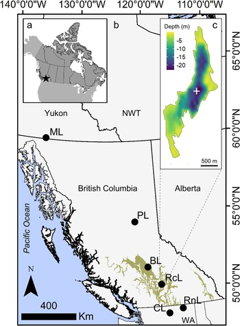
Roche Lake is a dimictic freshwater lake located on the Thompson Plateau of the southern interior region of British Columbia (elevation 1135 m; Fig. 1), ~25 km southeast of Kamloops, BC, and is within the dry and cool subzone of the Interior Douglas Fir (IDF) biogeoclimatic zone. It is a relatively small lake, with a surface area of 134 ha and a maximum depth of 23 m. The Roche Lake catchment is ~3500 ha, and four small lakes flow into Roche Lake via one intermittent inlet (Mushet et al., Reference Mushet, Reinhardt, Whitehouse and Cumming2022). Means of biweekly monitoring data collected between June 2015 and October of 2015 indicate it has a Secchi depth of 3.4 m, is meso-eutrophic (total dissolved phosphorus = 21 μg L−1), has a moderately high concentration of dissolved organic carbon (17 mg L−1), and experiences anoxia in the hypolimnion during the stratified period (~May–October) and following ice cover in the winter (~December–March) (Mushet et al., Reference Mushet, Laird, Leavitt, Maricle, Klassen and Cumming2019). The bathymetry is characterized by a deep (~23 m) central basin, a secondary relatively deep basin (~19 m) at the north end of the lake, and a gently sloping depth gradient towards the southwest end of the basin (Fig. 1). Much of the basin is also surrounded by a shallow, low relief shelf. The records from the nearest meteorological station to Roche Lake (~15 km) from the period AD 1987–2006 show that mean annual precipitation in the area is ~397 mm, and that mean winter and summer temperatures are ~ −3.1°C and 17.8°C, respectively (Mushet et al., Reference Mushet, Laird, Leavitt, Maricle, Klassen and Cumming2019). Vegetation in the catchment is dominated by Douglas fir (Pseudotsuga menziesii), Lodgepole pine (Pinus contorta), and spruce (Picea spp.), with some Trembling aspen (Populus tremuloides) and western redcedar (Thuja plicata) (Mushet et al., Reference Mushet, Laird, Leavitt, Maricle, Klassen and Cumming2019). The geology of the Thompson Plateau consists of mid-Eocene and Miocene basalts that are mantled with glacial drift, and granitic intrusions are also common throughout the region. Soils throughout the Roche Lake catchment are predominantly gray luvisols and dystric brunisols (Valentine et al., Reference Valentine, Sprout, Baker and Lavkulich1978).

Figure 1. Maps of the study region. a) Star indicates location of Roche Lake within the context of Canada (dark gray shading) and much of the United States (light gray shading). b) Black circles indicate location of Roche Lake (RcL), and additional sites in western Canada and Washington State, United States (WA) from Cumming et al. (2002; BL = Big Lake) and Steinman et al. (2014; ML = Marcella Lake, PL = Paradise Lake, CL = Castor Lake, RnL = Renner Lake) that were used to generate a composite of sedimentary δ18O for the past 2000 years for comparison with Roche Lake climate proxy data. Tan shading indicates the Interior Douglas Fir (IDF) biogeoclimatic zone. NWT is Northwest Territories, Canada. c) Inset map of the bathymetry of Roche Lake with the coring location for the composite sedimentary core (RLDM) indicated by the white +.
METHODS
Core collection and chronology
In June 2018, two overlapping sediment sequences were collected from the main deep basin of Roche Lake (Fig. 1) using a Livingstone piston corer with a 5.1-cm internal diameter (Glew et al., Reference Glew, Smol, Last, Last and Smol2001). The primary core was collected to capture the sediment–water interface, while a secondary core with a depth offset of 50 cm was collected ~2 m adjacent to the primary core to enable the development of a composite sedimentary sequence utilizing information from both cores. Cores were transported to cold storage (4°C) at Queen's University, subsequently split in the lab, and one half was sectioned at 0.5-cm intervals while the other was kept intact. The master sedimentary sequence was developed based on the overlap of the offset sequences identified from visible laminations, and high-resolution geochemical data obtained via μXRF. To determine whether the sediment–water interface of the piston core remained intact, we compared high-resolution diatom biostratigraphy to a 210Pb-dated gravity core collected from the same location to investigate for coherent changes in species composition (Mushet et al., Reference Mushet, Reinhardt, Whitehouse and Cumming2022). The final master sedimentary sequence (termed RLDM) from the cores from the deep basin of Roche Lake has a total length of 160 cm.
Pollen grains were isolated from raw sediment from five intervals in RLDM at the National Lacustrine Core Facility at the University of Minnesota, following standard protocols modified from Brown et al. (Reference Brown, Nelson, Mathewes, Vogel and Southon1989). The 14C activity from these five pollen extracts was measured at the Lawrence Livermore National Laboratory via accelerator mass spectrometry (AMS). The IntCal13 14C curve was used to calibrate 14C age estimates (Reimer et al., Reference Reimer, Bard, Bayliss, Beck, Blackwell, Bronk Ramsey and Buck2013), and a continuous age-depth model was developed using the Bayesian age-modeling package rbacon v. 2.4.2 (Blaauw and Christen, Reference Blaauw and Christen2011) in R (R Core Team, 2018). A 210Pb estimated date (11 cm = AD 1951) was also included in the chronology based on correlation of the high-resolution diatom biostratigraphy with a gravity core taken from the same location (Mushet et al., Reference Mushet, Reinhardt, Whitehouse and Cumming2022), while the surface level of the core (0–0.5 cm) was assigned to the year associated with coring.
Diatoms
Subfossil diatoms were analyzed at 1-cm intervals for the entirety of the core record. Samples were processed from raw sediment following standard procedures outlined in Laird et al. (Reference Laird, Das, Hesjedal, Leavitt, Mushet, Scott, Simpson, Wissel, Wolfe and Cumming2017). A minimum of 400 diatom valves were identified to the lowest possible taxonomic unit using a Leica DMRB microscope fitted with a 100× Fluotar objective and using differential interference contrast optics at 1000× magnification. Taxonomic references used included Krammer and Lange-Bertalot (Reference Krammer, Lange-Bertalot, Ettl, Gerloff, Heynig and Mollenhauer1986, Reference Krammer, Lange-Bertalot, Ettl, Gerloff, Heynig and Mollenhauer1988, Reference Krammer, Lange-Bertalot, Ettl, Gerloff, Heynig and Mollenhauer1991a, Reference Krammer, Lange-Bertalot, Ettl, Gärtner, Gerloff, Heynig and Mollenhauerb) and Cumming et al. (Reference Cumming, Wilson, Hall and Smol1995). An online taxonomic guide (Guiry and Guiry, Reference Guiry and Guiry2017; https://www.algaebase.org) was also consulted to ensure that updated synonymized species names were used when appropriate.
Chlorophyll-a
Concentrations of chlorophyll-a (Chl-a) and its associated degradation products were estimated using visible reflectance spectroscopy (VRS), following the methods outlined in Michelutti et al. (Reference Michelutti, Blais, Cumming, Paterson, Rhüland, Wolfe and Smol2010). For each sample, a small amount of freeze-dried sediment was sieved through a 125-μm screen, transferred into individual 12-mL glass vials, and analyzed for reflectance spectra using a FOSS NIR Model 6500 Rapid Content Analyzer. Sedimentary Chl-a concentrations were estimated from the spectral absorbance of wavelengths between 650 nm and 700 nm, based on its linear relationship to high-performance liquid chromatography-derived Chl-a (and derivatives) as defined in Michelutti et al. (Reference Michelutti, Blais, Cumming, Paterson, Rhüland, Wolfe and Smol2010). Loss-on-ignition was subsequently performed following the procedures of Dean (1974), and Chl-a data were normalized to percent organic matter to account for the possible influence of changes in sediment matrix on Chl-a concentrations. VRS analysis and loss-on-ignition were performed on the same sample intervals that were also used for diatom analysis.
Sediment geochemistry
Relative concentrations of trace elements were measured using a Cox Analytical Systems ITRAX® μXRF core scanner at the McMaster University Core Scanning Facility. Scans were completed using a molybdenum tube set to 30kV and 20mA, with a step size of 0.5 mm and a dwell time of 15 s. Raw data were averaged over 0.5-cm intervals, which is the same interval thickness used for diatom and Chl-a analysis, and these data are presented as either counts (cps) normalized to the sum of coherent and incoherent backscatter (for lithogenic elements; Kylander et al., Reference Kylander, Ampel, Wohlfarth and Veres2011), or as log-transformed element ratios (Weltje and Tjallingii, Reference Weltje and Tjallingii2008; Gregory et al., Reference Gregory, Patterson, Reinhardt, Galloway and Roe2019).
Here, the log-transformed ratio of calcium (Ca) to titanium (Ti) is used as a proxy for EM, which represents a combined influence of changes in mass flux via precipitation, and energy flux (e.g., solar irradiance, atmospheric heat). In lakes situated in arid to semiarid regions, lake-level drawdown throughout the warm season is often pronounced compared to lakes in more mesic areas (Campbell et al., Reference Campbell, Campbell and Hogg1994). Subsequent evapoconcentration of ions (including calcium) due to these seasonal changes in temperature leads to the precipitation of calcium carbonate (CaCO3), a process that is typically enhanced during periods of prolonged drought (Cohen, Reference Cohen2003). Moreover, the high modern pH (~8.5) and high Ca concentration (~33 mg L−1) suggest that Roche Lake can produce authigenic carbonates under the right conditions. While some calcium-limited systems may undergo carbonate precipitation during wet periods due to enhanced groundwater inputs (Shapley et al., Reference Shapley, Ito and Donovan2005; Nelson et al., Reference Nelson, Abbott, Steinman, Polissar, Stansell, Ortiz, Rosenmeier, Finney and Riedel2011), we note that previous work has associated warm and dry periods with carbonate precipitation in Roche Lake (Mushet et al., Reference Mushet, Reinhardt, Whitehouse and Cumming2022). In contrast, titanium (Ti) and potassium (K) are used as proxies for direct mass inputs to the lake from the watershed because they are strong indicators of lithogenic material (Cohen Reference Cohen2003; Kylander et al., Reference Kylander, Ampel, Wohlfarth and Veres2011). We note that while aeolian transport of lithogenic materials is an important source of sediment delivery to lakes in some regions (Chu et al., Reference Chu, Sun, Zhaoyan, Rioual, Qiang, Kaijun, Han and Liu2009), previous work in southern BC has shown that aeolian deposition rates are generally low (Owens and Slaymaker, Reference Owens and Slaymaker1997; Evans and Slaymaker, Reference Evans and Slaymaker2004). Hence, we expect the relative concentrations of Ti and K to increase during wetter periods due to enhanced runoff from the catchment.
Numerical analysis
Statistical analysis was undertaken to: 1) decompose the multivariate diatom data into temporal series representing major changes in community composition over the past 1800 years; 2) investigate temporal trends in the proxy data (diatoms, Chl-a, and μXRF); and 3) quantify the relative importance of changes in water level and erosional events on the main directions of change in diatom species composition, and total primary production in the core from Roche Lake. Because twentieth-century anthropogenic eutrophication of Roche Lake has overwhelmed other signals in the proxy data that are presumably related to long-term patterns in climate, the top 12 samples (i.e., 0–12 cm; after AD 1940) were eliminated for all following statistical analyses. This date was selected as a cutoff point based primarily on the ~80% increase in eutrophic Stephanodiscus taxa that was unprecedented within the context of the record (Mushet et al., Reference Mushet, Laird, Leavitt, Maricle, Klassen and Cumming2019).
Principal component analysis (PCA) was used to summarize changes in the diatom assemblages throughout the core. PCA was performed on square-root-transformed relative abundance data and included only abundant taxa (>2% relative abundance in at least one sample). Significant axes were identified using a scree plot with a broken-stick distribution as the null model. Generalized additive models (GAMs) were subsequently used to investigate trends in significant diatom PCA axes, key trace elements, and Chl-a data. GAMs allow for flexible relationships between a response variable and predictor(s), and are appropriate for paleoecological data where linear relationships are not necessarily expected (Simpson, Reference Simpson2018). In these models, age was used as the sole covariate, restricted maximum likelihood was used as the smoothness selection method, thin plate splines were used as the basis spline, and sedimentation times (yr cm−1) were used as observational weights to help account for heteroscedasticity in the data (Simpson, Reference Simpson2018).
Three additional GAMs were generated to quantify the influence of lake level (and accompanying changes in internal lake processes) and erosional inputs on diatom species composition and primary production. In addition to allowing the relationship between explanatory variable(s) and the response to change over time, the GAM method enables the contribution of each explanatory variable to the fitted response to be analyzed separately because of the additive structure of the models (Simpson and Anderson, Reference Simpson and Anderson2009). Here, the response variables over the past 1800 years were the diatom PC axis-1 scores (model 1), diatom PC axis-2 scores (model 2), and Chl-a (model 3). In each model, the explanatory variables were log (Ca/Ti) as a proxy for EM, with high values indicating low EM or more arid periods, and potassium (K; normalized to total backscatter) was selected as a proxy for erosional inputs. These two covariates (log (Ca/Ti) and K) had low correlations and were not significantly related (r = −0.05, p = 0.60). Following Simpson and Anderson (Reference Simpson and Anderson2009), a trend component (age) was also included in each model, using age as a third covariate. This was done to capture enough variance in the data, thereby reducing the possibility for unaccounted patterns in the data to influence estimates of importance of the other two covariates. The default Gaussian error distribution was used when modeling PCA axis scores, while a Gamma family was used when modeling Chl-a. For each of the three model covariates, k (the basis dimension, or the upper limit on the degrees of freedom) was set to 30 to ensure sufficient degrees of freedom to represent each covariate. All statistical analyses were carried out in R (R Core Team, 2018), using the packages vegan (Oksanen et al., Reference Oksanen, Guillaume Blanchet, Friendly, Kindt, Legendre, McGlinn and Minchin2020), rioja (Juggins, Reference Juggins2020), mgcv (Wood, Reference Wood2011; Wood et al., Reference Wood, Pya and Säfken2016), and gratia (Simpson and Oksanen, Reference Simpson and Oksanen2020).
RESULTS
Chronology
Details of the five AMS 14C dates are provided in Table 1. At 2σ, the bottommost age at 159.5-cm core depth is 1890–1730 cal yr BP (AD 60–220). The diatom biostratigraphy of the top 22 cm of RLDM matched that of the 210Pb-dated gravity core that was taken in the same location in 2016, which also enabled us to include a 210Pb estimated age in the final chronology (see Mushet et al., Reference Mushet, Reinhardt, Whitehouse and Cumming2022 for details). The Bayesian age-depth model estimated an age of 1778 cal yr BP (AD 172) at 160-cm core depth, resulting in an average resolution of ca. 11.5 years between samples for diatom and Chl-a analysis over the last ca. 1850 years. The RLDM age-depth model shows an approximately linear trend (Fig. 2), with the discrepancy between the topmost two 14C ages (Table 1, Fig. 2) attributable to the more complicated shape of the 14C calibration curve at younger ages. The Bacon program handles possible outliers well because it assumes that radiocarbon dates come from the heavy-tailed t-distribution (Trachsel and Telford, Reference Trachsel and Telford2017), so all ages were included in the final model.

Figure 2. Bayesian age-depth model for the Roche Lake composite core (RLDM) based on calibrated 14C ages. Top left panel: Markov Chain Monte Carlo iterations; top middle and right panels show prior (green lines) and posterior densities (gray fills) for mean accumulation rate and memory, respectively. Large bottom panel shows calibrated 14C ages and the age-depth model. The central red dotted line is the model based on the weighted mean age, the grayscale cloud represents age model probability, and is bounded by a 95% confidence interval (dashed gray line).
Table 1. Summary of the 14C dating results for the composite sediment core (RLDM) collected from Roche Lake. All 14C analyses were performed on pollen that was isolated from raw sediment at the LacCore Facility at the University of Minnesota. CAMS = Center for Accelerator Mass Spectrometry. * indicates date was obtained from 210Pb analyses of a gravity core taken from the same coring location in 2016, which was then correlated to the composite piston core using high-resolution diatom biostratigraphy (Mushet et al., Reference Mushet, Reinhardt, Whitehouse and Cumming2022).

Diatoms
In RLDM, both planktonic and benthic diatom taxa are important throughout, accounting for, on average, ~60% and 40% of the assemblage, respectively. The more dominant planktonic taxa are Lindavia lemanensis, Lindavia michiganiana, Fragilaria crotonensis, and Asterionella formosa. Several small Stephanodiscus species (S. cf. parvus, S. minutulus, S. hantzschii) are also present at lower abundances (<15%) during certain periods (excluding the top 12 cm). Benthic diatoms include small, benthic Fragilariaceae and several species within the Achnanthes, Amphora, Cymbella, and Navicula genera (Fig. 3).

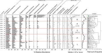
Figure 3. The diatom stratigraphy for RLDM from Roche Lake, plotted by composite core depth. Significant zonations based on stratigraphically constrained cluster analysis (CONISS) coupled with a broken-stick model are indicated by solid red lines. The zone above the dashed line represents twentieth-century eutrophication of Roche Lake and was removed from CONISS analysis. The MCA (Medieval Climate Anomaly; AD 900–1300) and LIA (Little Ice Age; AD 1450–1850) are shown for reference.
A stratigraphically constrained cluster analysis (CONISS; Grimm, Reference Grimm1987) based on the Hellinger distance (i.e., the Euclidean distance computed using Hellinger-transformed species data) coupled with a broken-stick model (Bennett, Reference Bennett1996) identified five significant diatom zones (Fig. 3). Diatom Zone 1 (AD 172–596) consists of moderate abundances of L. michiganiana and benthic Fragilariaceae (~20% on average), and low abundances of Asterionella formosa (<10%). Diatom Zone 2 (AD 596–947) is characterized by subtle increases in Cymbella spp., Cymbellafalsa diluviana, and a decline in Asterionella formosa. When relative abundances of planktonic taxa were analyzed without the inclusion of benthic taxa, F. crotonensis (and S. niagarae to some extent) displace L. michiganiana during this time (Supplemental Figure S1). In Diatom Zone 3 (AD 947–1367), L. lemanensis and L. michiganiana become more abundant, each fluctuating between 25–30%, accompanied by declines in F. crotonensis and some benthic taxa, including Cymbella spp., Cymbellafalsa diluviana, and the benthic Fragilariaceae. In Diatom Zone 4 (AD 1367–1730), Asterionella formosa, S. hantzschii, and S. cf. parvus are all present at low abundances (<10%), and L. lemanensis abundances decline to ~20%, except for a peak at ca. AD 1600. Finally, Diatom Zone 5 (AD 1730–1941) is characterized by higher relative abundances of F. crotonensis (25–30%), and declines in L. michiganiana and small Stephanodiscus spp. The top of the core (after AD 1941) is dominated by S. cf. parvus, representing anthropogenic eutrophication of Roche Lake (Mushet et al., Reference Mushet, Laird, Leavitt, Maricle, Klassen and Cumming2019).
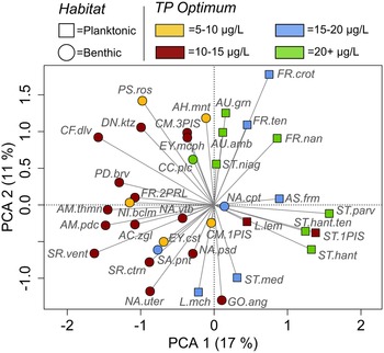
Diatom PCA axis-1 and axis-2 capture 17% and 11% of the total variance in the assemblage, respectively (Fig. 4), and both axes were significant. PC axis-1 represents a gradient of change from an assemblage characterized by benthic taxa with low total phosphorus (TP) optima (negative axis-1 loadings), towards an assemblage characterized by predominantly planktonic taxa (small Stephanodiscus spp., Asterionella formosa) with higher TP optima (positive axis-1 loadings; Fig. 4). Diatom PC axis-2 largely represents the balance between one of the main planktonic taxa, L. michiganiana (associated with negative axis-2 loadings), and F. crotonensis and several benthic taxa that have positive axis-2 loadings (Fig. 4). PC axis-2 does not differentiate as strongly between taxa with high and low TP optima in comparison to PC axis-1.

Figure 4. Principal components analysis (PCA) biplot showing diatom species scores for the high-resolution analysis of the composite core from Roche Lake (RLDM). Taxa are coded by habitat type and total phosphorus (TP) optima based on the 251-lake calibration set presented in Cumming et al. (Reference Cumming, Laird, Gregory-Eaves, Simpson, Sokal, Nordin and Walker2015). AC.zgl = Achnanthes ziegleri, AH.mnt = Achnanthidium minutissimum, AM.pdc = Amphora pediculus, AM.thmn = Amphora thumensis, AS.frm = Asterionella formosa, AU.amb = Aulacoseira ambigua, AU.grn = Aulacoseira. granulata, CC.plc = Cocconeis placentula sensu lato, CF.dlv = Cymbellafalsa diluviana, CM.1PIS = Cymbella sp. 1 PISCES, CM.3PIS = Cymbella sp. 3 PISCES, L.lem = Lindavia lemanensis, DN.ktz = Denticula kuetzingii, EY.cst = Encyonopsis cesatti, EY.mcph = E. microcephala, FR.2PRL = Fragilaria sp. 2 PIRLA, FR.crot = F. crotonensis, FR.nan = F. nanana, FR.ten = F. tenera, GO.ang = Gomphonema angustum, L.mch = Lindavia michiganiana, NA.cpt = Navicula cryptotenella, NA.psd = Na. pseudoventralis, NA.uter = Na. aff. utermoehlii, NA.vtb = N. vitabunda, NI.bclm = Nitzschia bacillum, PD.brv = Pseudostaurosira brevistriata, PS.ros = Psammothidium rosenstockii, SA.pnt = Staurosirella pinnata, SR.ctrn = Staurosira construens, SR.vent = Staurosira construens var. venter, ST.1PIS = Stephanodiscus sp. 1 PISCES, ST.hant = Steph. hantzschii, ST.hant.ten = Steph. hantzschii f. tenuis, ST.med = Steph. medius, ST.niag = Steph. niagarae, ST.parv = Steph. parvus.
Prior to AD 600, PC axis-1 scores are variable, but show a subtle increasing trend after this time (Fig. 5g). At ca. AD 1370, PC axis-1 begins to show a decreasing trend which persists until the top of the sequence except for a maximum at ca. AD 1730. Diatom PC axis-2 scores are elevated between AD 600 and AD 950 (Fig. 5d), after which they show a declining trend until AD 1350. After AD 1350, PC axis-2 scores again show an increasing trend until AD 1800, where they begin to show a declining trend that persists to the beginning of the sequence.

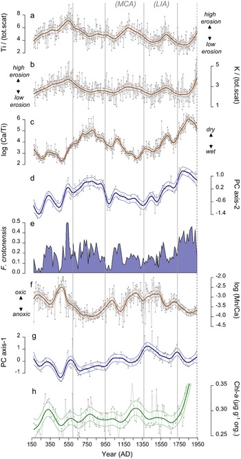
Figure 5. Summary of proxy data from the composite core from Roche Lake (RLDM), plotted by age (Year AD). Bold lines through each time-series (except for Fragilaria crotonensis) are trends and associated 95% confidence intervals estimated using generalized additive models (GAMs). Zonations determined from the stratigraphically constrained cluster analysis (CONISS) performed on the diatom relative abundance data are indicated by vertical gray lines. The MCA (Medieval Climate Anomaly; AD 900–1300) and LIA (Little Ice Age; AD 1450–1850) are shown for reference. a) Titanium (Ti) normalized to the sum of coherent and incoherent scatter (tot.scat), b) potassium (K) normalized to the sum of coherent and incoherent scatter (tot.scat), c) log-ratio of calcium (Ca) to titanium (Ti), d) diatom principal component axis-2 scores (PC-axis 2), e) proportion of F. crotonensis relative to total plankton, f) log-ratio of manganese (Mn) to calcium (Ca), g) diatom principal component axis-1 scores (PC-axis 1), h) chlorophyll-a (Chl-a) normalized to the proportion of organic matter.
Chlorophyll-a (Chl-a)
Chl-a displays only subtle changes through time, with distinct maxima in concentrations occurring at AD 340 and ca. AD 1300, and more subtle peaks in concentration at AD 550 and AD 800 (Fig. 5h). After AD 1750, Chl-a displays an increasing trend, a pattern that persists to the top of the core.
Geochemical data (μXRF via ITRAX)
Throughout RLDM, Ti, K, and Fe are positively correlated with each other (r = 0.48 to 0.57), while Ca, Sr, and Mn are highly correlated (r = 0.87 to 0.97), and only weak correlations exist between these two groups of elements (Supplemental Table 1, Supplemental Figure S2). This relationship is consistent with the authigenic nature of carbonates in RLDM because Ca and Sr often coprecipitate when lake waters become supersaturated with CaCO3 (Kylander et al., Reference Kylander, Ampel, Wohlfarth and Veres2011). Often present in lake sediments as an oxide or hydroxide, Mn is a redox-sensitive element that can form an insoluble precipitate when lake bottom waters are well-oxygenated (Aguilar and Nealson, Reference Aguilar and Nealson1998; Kylander et al., Reference Kylander, Ampel, Wohlfarth and Veres2011). However, Mn can also be incorporated into carbonates (Friedl et al., Reference Friedl, Wehrli and Manceau1997). Given the high correlation between Ca, Sr, and Mn (Supplemental Table 1, Supplemental Figure 2), raw Mn counts were normalized to Ca to enable inferences of Mn oxide/hydroxide content as a potential proxy of deep-water oxygen conditions. The positive associations between Ti, K, and Fe are consistent with allochthonous origins of these elements, although only Ti and K are used as erosional indices because Fe can also be influenced by lake redox conditions (Davies et al., Reference Davies, Lamb, Roberts, Croudace and Rothwell2015). While a strong negative correlation between erosional indices and carbonate content may be expected, we note that our high-resolution (0.5 mm) geochemical data can capture differences in the temporal scale at which erosional events occur compared to the prolonged warm and/or dry periods that drive carbonate precipitation in lakes in semiarid regions. Moreover, variation in the seasonal timing of precipitation events (e.g., spring freshet compared to strong summer and fall storms) can generate different rates of lake-wide sediment delivery (Schiefer et al., Reference Schiefer, Menounos and Slaymaker2006). Both of these processes may contribute to the low degree of correlation between erosional indices and carbonate content.
Ca (presented as log (Ca/Ti)) is generally low until AD 450, after which time it shows an increasing trend that persists until AD 800 (Fig. 5c). Except for a peak at AD 1100, values are generally low between AD 800 and AD 1550. Post-AD 1350, log (Ca/Ti) shows an increasing trend, with smaller maxima occurring at AD 1650 and AD 1850. Variations in Ti and K are generally smaller in magnitude compared to log (Ca/Ti). Both Ti and K show subtle peaks at AD 550, AD 1200, and AD 1600, and minimums at AD 750, AD 1050, and AD 1450, and were low between AD 1750 and AD 1850 (Fig. 5a, b).
Generalized additive models (GAMs)
In the three GAMs that were generated to quantify the influence of water level and erosional inputs on diatom species composition (diatom PC axis-1 and - 2; models 1 and 2, respectively) and total primary production (Chl-a; model 3), the trend component that used age as a covariate was always significant (Table 2). In all three models, log (Ca/Ti), a proxy for EM, was also always a significant predictor, while K (normalized to the sum of coherent and incoherent scatter), a proxy for erosional inputs, was not significant in any of the models. The deviance explained in the models was 66% for model 1, 75% for model 2, and 63% for model 3 (Table 2). Because K was not a significant predictor in any of the models, hereafter we focus primarily on the relationship between log (Ca/Ti) and the three response variables.
Table 2. Summaries for the generalized additive models (GAMs) fitted to the diatom PCA axis-1 and axis-2 scores, and chlorophyll-a. EDF = effective degrees of freedom; Ref. df = reference degrees of freedom, F = F-statistic, p = p-value of each model term.

The smooth function for log (Ca/Ti) showed a non-linear relationship with diatom PC axis-1 scores and indicated a positive effect on PC axis-1 when log (Ca/Ti) was low (between 2 and 3); whereas the effect of log (Ca/Ti) on PC axis-1 was less pronounced, but negative at values >3 (Fig. 6a). This pattern was evident in the time series of the contribution of log (Ca/Ti) to the fitted PC axis-1 scores, which showed significant contributions to the minima in PC axis-1 scores at AD 250, AD 450, and AD 1300 (Fig. 7a). The smooth function between log (Ca/Ti) and PC axis-2 scores was linear (edf = 1) and positive, indicating a strong relationship between the two (Fig. 6b). Indeed, the contribution of log (Ca/Ti) to the fitted PC axis-2 scores closely resembled the final model predictions when all model covariates were used (Fig. 7c, d). Finally, the relationship between log (Ca/Ti) and Chl-a was generally positive (Fig. 6c), although this relationship was more pronounced when log (Ca/Ti) values were low (<3). This was evident when examining the time series of the contribution of log (Ca/Ti) to the fitted Chl-a values, where log (Ca/Ti) made significant contributions to the minima in Chl-a at AD 250, AD 450, and AD 1300, while the relationship between the two was weak for the remainder of the record, given the confidence intervals bounded the zero line (i.e. not statistically different from the intercept; Fig. 7e). The smooth functions and contribution to the final fitted GAMs for all other model covariates (i.e., complete model outputs) are shown in Supplemental Figures S3–S5.
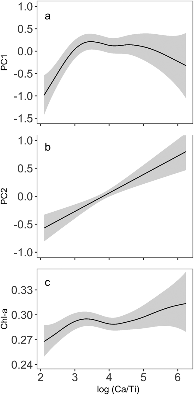
Figure 6. Fitted smooth functions for log (Ca/Ti) from the three separate generalized additive models (GAMs) that used: a) diatom principal component axis-1 (PC axis-1), b) diatom principal component axis-2 (PC axis-2), and c) chlorophyll-a (Chl-a) as response variables. Pointwise confidence intervals (95%) for each model are indicated by gray bands.
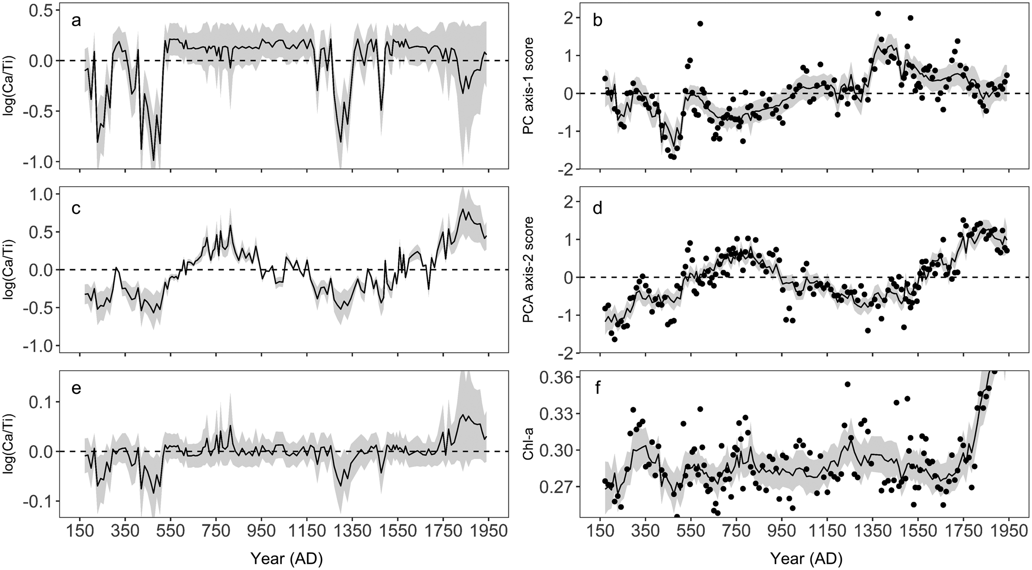
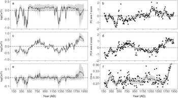
Figure 7. The contribution of log (Ca/Ti) to each of the three generalized additive models (GAMs) and observed and GAM-fitted values using all model covariates for each of the three models. a) Contribution of log (Ca/Ti) to the fitted diatom principal component axis-1 (PC axis-1) scores, b) observed and final GAM-fitted values for diatom principal component axis-1 (PC axis-1) scores, c) the contribution of log (Ca/Ti) to the fitted diatom principal component axis-2 (PC axis-2) scores, d) observed and final GAM-fitted values for diatom principal component axis-2 (PC axis-2) scores, e) contribution of log (Ca/Ti) to the fitted chlorophyll-a (Chl-a) values, f) observed and final GAM fitted values for chlorophyll-a (Chl-a) values. Gray bands represent 95% pointwise confidence intervals. For panels a, c, and e, where the band encompasses the dashed zero line, the contribution of log (Ca/Ti) is not significantly different from the intercept.
DISCUSSION
The primary goal of this study was to understand how diatom assemblages and primary production changed as function of past changes in EM, and whether EM effects on these properties were driven mostly by lake level and associated lake–atmosphere energy exchange, or changes in landscape properties and erosional inputs. Analysis of geochemical and biological proxies in RLDM spanning the past ca. 1800 years revealed an extended period of reduced EM between ca. AD 600 and AD 950, and a declining trend in EM since ca. AD 1350. More subtle variations in erosional indices occurred throughout the record, although GAMs revealed that this had less of an effect on diatom species composition and total algal production when compared to more direct impacts of atmospheric forcing on lake thermal properties that accompanied changes in EM. Detailed interpretations of changes in the diatom assemblages are used to highlight changes in lake function, and the GAMs are used to provide a more thorough understanding of linkages with EM. This is followed by a comparison with a previously published synthesis of paleoclimate proxies throughout the Pacific Northwest (PNW), with an emphasis on understanding patterns during the MCA and LIA. In this discussion, modern climate refers to climate conditions inferred from the diatom and geochemical data during the pre-eutrophication period of Roche Lake (Diatom Zone 5; ca. AD 1730–1940).
Diatom Zone 1 (ca. AD 170–600)
The main features of Diatom Zone 1 include the presence of Asterionella formosa (albeit at relative abundances <15%), with peaks in F. crotonensis occurring at AD 350 and AD 550, and a maximum in several benthic taxa at AD 450 (Fig. 3). We infer this zone to represent generally cooler and/or wetter conditions relative to modern. In WNA, A. formosa has been identified as a taxon that blooms prior to strong summer thermal stratification (Interlandi et al., Reference Interlandi, Kilham and Theriot1999), a pattern that has also been documented in other regions (e.g., Maberly et al., Reference Maberly, Hurley, Butterwick, Corry, Heaney, Irish, Jaworski, Lund, Reynolds and Roscoe1994). However, the presence of A. formosa in lake sediment records from WNA has also been linked with enhanced silica (Si) and nitrogen (N) inputs during periods of high winter precipitation and enhanced spring runoff (Bracht-Flyr and Fritz, 2012). Hence, the presence of A. formosa could represent enhanced spring mixing conditions, a wetter winter/spring period, or both. Enhanced mixing is consistent with high deep-water oxygen as suggested by higher Mn/Ca throughout this zone (except the minimum at ca. AD 350; Fig. 5f), while a wetter winter/spring is consistent with generally higher erosional indices during this time (Fig. 5a, b). Although it is difficult to disentangle the relative importance of precipitation patterns versus temperature, the presence of A. formosa is consistent with higher EM during this time.
Within this zone, GAMs indicate two brief periods of exceptionally high EM, indicated by the lowest log (Ca/Ti) within the record, which had significant impacts on diatom species composition and total algal production (Fig. 7a, c, e). Minima in diatom PC axis-1 scores (Fig. 5g) corresponded to peaks in several benthic taxa, including some benthic Fragilariaceae, and Amphora and Achnanthes taxa. Given that these taxa have lower TP optima (<15 μg L−1; Fig. 4), and GAMs indicated that these maxima in water level were responsible for low Chl-a (Fig. 7e), this diatom response could indicate a period of reduced primary production. However, wetter conditions could be expected to enhance nutrient delivery to the lake (Schindler et al., Reference Schindler, Bayley, Parker, Beaty, Cruikshank, Fee, Schindler and Stainton1996), favoring higher production. An alternative explanation for this trend in diatom PC axis-1 scores is that brief periods of exceptionally high moisture altered benthic habitat by a reduction in water clarity, likely related to an enhanced delivery of particles and solutes from the watershed (Weyhenmeyer et al., Reference Weyhenmeyer, Willén and Sonesten2004). The benthic Fragilariaceae often maintain a competitive advantage in low-light environments (Lotter and Bigler, Reference Lotter and Bigler2000), while Hofman et al. (Reference Hofmann, Geist, Nowotny and Raeder2020) showed that several species of Amphora were also tolerant of lower light in small, alpine lakes. Hence, reduced light availability could have limited total algal production during this period, but provided a competitive advantage to taxa adapted to low-light conditions. It is also possible that these periods represent exceptionally cool conditions that could also have limited primary production (Ho and Michalak, Reference Ho and Michalak2020). Nevertheless, the GAMs indicate that this zone was punctuated by abrupt variations in EM that had an important control on lake function.
Diatom Zone 2 (ca. AD 600–950)
The main features of Diatom Zone 2 are sustained, high relative abundances of F. crotonensis (at ~25–30%), a reduction in L. michiganiana and Asterionella formosa, and an increase in some benthic taxa including Cymbella spp. and Cymbellafalsa diluviana. We infer that these shifts in species composition represent a prolonged period of reduced EM, like that in Zone 5 (i.e., modern). Analysis of sediment trap material from the profundal zone of Elk Lake (Minnesota, USA) showed that F. crotonensis was often abundant in the spring and early summer (likely in the metalimnion) in years characterized by a short period of spring mixing and rapid transition to summer thermal stratification (Bradbury, Reference Bradbury1988; Bradbury et al., Reference Bradbury, Cumming and Laird2002). In Elk Lake, this pattern likely arose because F. crotonensis is a good competitor when limnetic phosphorus (P) concentrations are low (Kilham and Kilham, Reference Kilham and Kilham1978; Bradbury et al., Reference Bradbury, Cumming and Laird2002), a condition that occurs once spring mixing and associated nutrient circulation ceases. However, it is important to note that the phenology of F. crotonensis may be variable. In WNA, Interlandi et al. (Reference Interlandi, Kilham and Theriot1999) showed that F. crotonensis formed metalimnetic blooms late in the summer, while St. Jacques et al. (Reference St. Jacques, Cumming and Smol2009) showed that F. crotonensis bloomed during the spring and the summer period based on associations with seasonal laminations in a sediment core from a lake in west-central Minnesota. Given that several Cymbella spp. and Achnanthidium minutissimum increased during this zone, genera that are often epilithic and/or epipelic and may be adapted to water movements in the shallowest portion of the littoral zone (Passy, Reference Passy2007; Hofmann et al., Reference Hofmann, Geist, Nowotny and Raeder2020), we suggest that F. crotonensis signifies enhanced thermal stratification that accompanies reduced lake level during warm and dry periods. This inference is also supported by the loss of Asterionella formosa during this period. The reduced relative abundance of L. michiganiana during this period is somewhat difficult to reconcile given that it is considered a late summer epilimnetic bloomer in WNA lakes (Bracht-Flyr and Fritz, Reference Bracht-Flyr and Fritz2012; Whitlock et al., Reference Whitlock, Dean, Fritz, Stevens, Stone, Power, Rosenbaum, Pierce and Bracht-Flyr2012), although St. Jacques et al. (Reference St. Jacques, Cumming and Smol2009) found that it had variable phenological characteristics. It is possible, however, that reduced abundances of L. michiganiana during this period represent a loss of planktonic habitat or limited nutrient supply to the epilimnion under stronger thermal stratification (e.g., Wilhelm and Adrian, Reference Wilhelm and Adrian2008).
Geochemical indices of erosion and deep-water oxygenation, and results from the GAMs support our interpretation of warm and dry conditions during this period. The strong, positive relationship between diatom PC axis-2 scores and log (Ca/Ti) (Fig. 6b) suggests EM as an important driver of taxa associated with PC axis-2, which was also reflected in the ability of log (Ca/Ti) to predict PC axis-2 scores that closely resembled model predictions when all covariates were used (Fig. 7c, d). Strong correlations between F. crotonensis and both PC axis-2 scores (r = 0.74, p < 0.001) and Ca (r = 0.56, p < 0.001; Fig. 5c, e) confirm that F. crotonensis is an important driver of the patterns in PC axis-2, as well as its affinity for high log (Ca/Ti). Reduced oxygenation of hypolimnetic waters indicated by low Mn/Ca during this time is also consistent with enhanced stratification of the water column (Fig. 5f), while generally lower erosional indices are consistent with reduced delivery of lithogenic material from the catchment, as would occur under dry conditions (Fig. 5a, b; Davies et al., Reference Davies, Lamb, Roberts, Croudace and Rothwell2015).
Little change in total algal production occurred during this warm, dry period (Fig. 5h), suggesting that reduced deep-water oxygen was driven primarily by an alteration to lake mixing patterns, and not enhanced decomposition of algal biomass. Moreover, the lack of a significant relationship between Chl-a and log (Ca/Ti) (Fig. 7e) indicates that carbonate precipitation driven by elevated photosynthetic activity (Kelts and Hsü, Reference Kelts, Hsü and Lerman1978) was not the paramount process driving sedimentary Ca concentrations.
Diatom Zone 3 (ca. AD 950–1370): The Medieval Climate Anomaly (MCA)
Diatom Zone 3 broadly corresponds to the MCA (ca. AD 900–1300), a period of enhanced aridity in many parts of WNA that has been linked with changes in solar and volcanic radiative forcing anomalies and Pacific Ocean–atmosphere processes (Cook et al., Reference Cook, Woodhouse, Eakin, Meko and Stahle2004, Reference Cook, Seager, Heim, Vose, Herweijer and Woodhouse2010; Mann et al., Reference Mann, Zhang, Rutherford, Bradley, Hughes, Shindell, Ammann, Faluvegi and Ni2009). One of the main features of this zone is a rise in the proportion of L. lemanensis (Fig. 3). Previous paleoecological research has consistently identified this taxon as a late summer bloomer (Bradbury, Reference Bradbury1988; Interlandi et al., Reference Interlandi, Kilham and Theriot1999; St. Jacques et al., Reference St. Jacques, Cumming and Smol2009), and its dominance has been interpreted to represent prolonged summer-like conditions in lakes throughout WNA (Bracht et al., Reference Bracht, Stone and Fritz2008; Whitlock et al., Reference Whitlock, Dean, Rosenbaum, Stevens, Fritz, Bracht and Power2008; Bracht-Flyr and Fritz, Reference Bracht-Flyr and Fritz2012). However, declines in several benthic taxa, and lower relative abundances of F. crotonensis on average when compared to the previous zone suggest a transition to slightly cooler and/or wetter conditions, inconsistent with inferences of climate based on the current understanding of L. lemanensis autecology.
The geochemical proxies and the GAMs indicate alternative mechanisms could be responsible for the changes in diatom species composition in this zone. Declining log (Ca/Ti) and its associated control on declining diatom PC axis-2 scores (Figs. 5c, 7c, d) are consistent with an increase in EM, which is also supported by a local maximum in erosional indices at ca. AD 1200 (Fig. 5a, b). Despite L. lemanensis often being associated with prolonged summer conditions, Whitlock et al. (Reference Whitlock, Dean, Fritz, Stevens, Stone, Power, Rosenbaum, Pierce and Bracht-Flyr2012) noted that in lakes on the Beartooth Plateau (northwest USA), the depth of the epilimnion influenced the distribution of Cyclotella sensu lato species, where L. lemanensis was associated with lakes with the deepest mixing depths, and smaller taxa such as C. ocellata were associated with lakes with shallower mixing depths. Therefore, the increase in L. lemanensis could be explained by a deeper mixed surface layer generated by slightly cooler conditions relative to the previous more arid period, consistent with the rise in Mn/Ca (Fig. 5f) that indicates more oxic conditions. It is also possible that a rise in lake level during this period provided additional planktonic habitat for L. lemanensis. However, the summer season would have needed to remain sufficiently long for this taxon to bloom.
Diatom Zone 4 (ca. AD 1370–1730): The Little Ice Age (LIA)
Diatom Zone 4 broadly coincided with the LIA (ca. AD 1450–1840). The main feature of this zone was an increase in the abundance of small Stephanodiscus spp., Asterionella formosa, and a decline in L. lemanensis (Fig. 3). Previous work has shown that small Stephanodiscus (e.g., S. parvus, S. minutulus) often bloom during isothermal mixing during spring to early summer (Bradbury, Reference Bradbury1988; Interlandi et al., Reference Interlandi, Kilham and Theriot1999; St. Jacques et al., Reference St. Jacques, Cumming and Smol2009) when nutrients are redistributed throughout the water column, a pattern that has been attributed to their preference for Si:P <1 (Kilham and Kilham, Reference Kilham and Kilham1978). Hence, we infer that this zone represents generally cooler conditions, with a more prolonged mixing period early in the ice-free period, which is also consistent with the return of A. formosa during this time. High Mn/Ca during the first half of this zone (ca. AD 1370–1550; Fig. 5f) is consistent with enhanced water column circulation and subsequent oxygenation of the bottom waters, although this was interrupted by a brief period of anoxia (also signified by a peak in F. crotonensis) at ca. AD 1600. Moreover, despite inferences of cooler spring/early summer temperatures during this period, an increasing trend in log (Ca/Ti), and erosional indices (primarily Ti) that were lower on average in comparison to the MCA, suggest that the potentially cooler conditions during this time were also accompanied by a trend towards reduced total precipitation.
Diatom Zone 5: Modern/pre-eutrophication (AD 1730–1940)
Diatom Zone 5 is inferred to represent a return to warm and dry conditions based on a continued increase in log (Ca/Ti) that drove an increase in diatom PC axis-2 scores (Figs. 5c, 7c, d), and a coinciding reduction in water column ventilation (Fig. 5f). The rise in F. crotonensis in this zone occurs at the expense of the relative abundance of small Stephanodiscus spp. (Fig. 3), consistent with a shorter and/or warmer spring/early summer season as interpreted in Diatom Zone 2.
One prominent feature within this zone was an increase in Chl-a that exceeded the concentrations observed during the previous ca. 1600 years (Fig. 5h). The timing of this increase in Chl-a is sufficiently old that it should not represent diagenetic processes (Rydberg et al., Reference Rydberg, Cooke, Tolu, Wolfe and Vinebrooke2020). This increase in algal production is not reflected in the diatoms, given that little change in total diatom concentration occurs at this time (Fig. 3). This is in contrast with the subsequent zone (post-AD 1940; eliminated from all statistical analysis) where diatom concentrations increase up to fourfold in response to twentieth-century cultural eutrophication of Roche Lake (Mushet et al., Reference Mushet, Laird, Leavitt, Maricle, Klassen and Cumming2019). It is possible that the more arid conditions inferred for Zone 5 provided other phototrophic groups such as cyanobacteria (Paerl and Huisman, Reference Paerl and Huisman2008) with a competitive advantage, although it is not certain why a similar pattern was not observed in Diatom Zone 2 (ca. AD 600–950). However, the geochemical data (Ti, log (Ca/Ti)) do indicate that modern aridity may have been more pronounced than the AD 600–950 period, which could lead to unexpected changes in algal composition, although further analysis would be required to address this possibility. Finally, while elevated Chl-a could indicate that carbonate precipitation was driven by photosynthetic activity, the effect of log (Ca/Ti) on Chl-a is highly uncertain during this period (Fig. 7e), suggesting that EM likely remained the paramount driver of carbonate precipitation during this time.
Regional patterns in paleoclimate
The Roche Lake record is characterized by centennial-scale fluctuations in EM and patterns in lake mixing that are associated with changes in climate and seasonality. Two important periods of environmental change are captured within RLDM; the MCA (ca. AD 900–1300) and LIA (ca. AD 1450–1850). From a paleoclimate perspective, the MCA and LIA are of interest because of their expression across many parts of the globe (Mann et al., Reference Mann, Zhang, Rutherford, Bradley, Hughes, Shindell, Ammann, Faluvegi and Ni2009), and because the MCA has been proposed to serve as a conservative analog for future droughts in some regions (Woodhouse et al., Reference Woodhouse, Meko, MacDonald, Stahle and Cook2010). Strong evidence for conditions during the MCA that were warm and dry relative to modern has come from tree-ring analyses throughout the semiarid southwestern United States, while the LIA was characterized by cooler conditions (Cook et al., Reference Cook, Woodhouse, Eakin, Meko and Stahle2004, Reference Cook, Seager, Heim, Vose, Herweijer and Woodhouse2010). However, inferences of EM based on our analysis of RLDM reveal more complex patterns. Specifically, the beginning of the prolonged period of reduced EM (Diatom Zone 2; ca. AD 600–950) predates the beginning of the MCA by ca. 300 years (Fig. 5c). Moreover, geochemical data indicated that EM was increasing during the MCA and decreasing during the LIA.
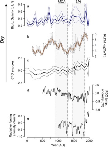
In BC and much of the PNW, La Niña, the negative phase of ENSO, is characterized by cooler spring temperatures and generally increased winter and spring precipitation (Fleming and Whitfield, Reference Fleming and Whitfield2010). In contrast, the southwestern portion of the United States generally experiences warmer and drier conditions during La Niña (Cole et al., Reference Cole, Overpeck and Cook2002). Indeed, the MCA has been linked to a prolonged La Niña-like state, thought to be driven by enhanced radiative forcing due to changes in solar irradiance and volcanic activity that led to the development of a stronger east–west sea-surface temperature gradient in the tropical Pacific (Mann et al., Reference Mann, Cane, Zebiak and Clement2005, Reference Mann, Zhang, Rutherford, Bradley, Hughes, Shindell, Ammann, Faluvegi and Ni2009; Cook et al., Reference Cook, Seager, Heim, Vose, Herweijer and Woodhouse2010). Hence, increased EM could have occurred in the PNW during the MCA. A synthesis of lake sediment oxygen-isotope records throughout the PNW documented patterns in EM consistent with this scenario where δ18O trends in lakes from northern Washington, BC, and southwest Yukon Territory indicated, on average, higher lake levels throughout the MCA (AD 900–1300) compared to the LIA (AD 1450–1850) (Steinman et al., Reference Steinman, Abbott, Mann, Ortiz, Feng, Pompeani, Stansell, Anderson, Finney and Bird2014). The trends in the Roche Lake log (Ca/Ti) record, as well as diatom-inferred salinity in a core from Big Lake in south-central BC, where elevated salinity is interpreted to represent enhanced evapoconcentration of ions and lake level drawdown (Fig.1; Cumming et al., Reference Cumming, Laird, Bennett, Smol and Salomon2002), are consistent with the patterns observed in sedimentary δ18O presented in Steinman et al. (Reference Steinman, Abbott, Mann, Ortiz, Feng, Pompeani, Stansell, Anderson, Finney and Bird2014), where EM was lower on average during the LIA relative to the MCA (Fig. 8). We also compared these records to a multi-proxy reconstruction of the Pacific Decadal Oscillation (PDO) over the central North Pacific region (Mann et al., Reference Mann, Zhang, Rutherford, Bradley, Hughes, Shindell, Ammann, Faluvegi and Ni2009). The PDO is considered a multidecadal response to ENSO (e.g., Newman et al., Reference Newman, Compo and Alexander2003), and warming of the central north Pacific (the negative phase of the PDO) is associated with La Niña-like conditions, while a cooling (the positive phase of the PDO) is associated with El Niño-like conditions. Hence, the more positive sea-surface temperature anomalies in the north Pacific during the MCA, and negative sea-surface temperature anomalies during the LIA, are also broadly consistent with the proposed connection between ENSO dynamics and hydroclimate during these climatic periods (Fig. 8).

Figure 8. Synthesis of climate proxy data over the past 2000 years from lakes from Western Canada and Washington State, USA. a) Diatom-inferred salinity from Big Lake in south-central BC (Fig. 1; Cumming et al., Reference Cumming, Laird, Bennett, Smol and Salomon2002). The smooth bold and light-colored lines are GAM estimated trends and 95% confidence intervals, respectively; b) Roche Lake composite core (RLDM) log-ratio of calcium to titanium. The smooth bold and light-colored lines are GAM estimated trends and 95% confidence intervals, respectively; c) composite of z-scored δ18O in sediment cores from several lakes throughout the Pacific Northwest (Fig. 1; Steinman et al., Reference Steinman, Abbott, Mann, Ortiz, Feng, Pompeani, Stansell, Anderson, Finney and Bird2014). Light-colored lines represent the 95% confidence interval based on assessment of age model uncertainty; d) north Pacific Decadal Oscillation (PDO) region sea-surface temperature reconstruction of Mann et al. (Reference Mann, Zhang, Rutherford, Bradley, Hughes, Shindell, Ammann, Faluvegi and Ni2009), which is averaged over 22.5°N–57.5°N, 152.5°E–132.5°W; e) 25-year moving average of total radiative forcing anomalies presented in Steinman et al. (Reference Steinman, Abbott, Mann, Ortiz, Feng, Pompeani, Stansell, Anderson, Finney and Bird2014), based on data from Crowley (Reference Crowley2000). Shading indicates the extent of the Medieval Climate Anomaly (MCA; AD 900–1300) and the Little Ice Age (LIA; AD 1450–1850).
In RLDM from Roche Lake, however, inferences of paleoclimate based on diatom species composition are not entirely consistent with these expected changes in ENSO during the MCA and LIA. While the rise in L. lemanensis during the MCA could have been caused by either a deeper mixed surface layer, a rise in water level, or both (relative to the previous zone), the warm season must have remained sufficiently long for it to bloom. Moreover, the presence of small Stephanodiscus spp. throughout most of the LIA is inconsistent with shorter/warmer El Niño-like spring seasons. This discrepancy could arise due to a complex (and possibly antagonistic) interaction between the direct influence of enhanced radiative forcing and the indirect influence of more La Niña-like conditions during the MCA, and reduced radiative forcing and El Niño-like conditions during the LIA (Fig. 8). Previous paleoecological studies in southern BC have also provided evidence for changes in aridity counter to those based on both the metanalysis of sedimentary δ18O presented in Steinman et al. (Reference Steinman, Abbott, Mann, Ortiz, Feng, Pompeani, Stansell, Anderson, Finney and Bird2014) and the geochemical data in RLDM from Roche Lake, further highlighting the complexities associated with these periods. For example, based on analysis of charcoal and Chara oospores in a sediment sequence from Dog Lake in southeast BC, Hallett et al. (Reference Hallett, Mathewes and Walker2003) provided evidence for more pronounced fire activity and reduced lake levels during the MCA relative to much of the LIA, much like the pattern in sedimentary charcoal shown by Lucas and Lacourse (Reference Lucas and Lacourse2013) in a core taken from a lake on the southwest coast of BC.
An additional important observation based on the analysis of RLDM was that the period preceding the MCA (Diatom Zone 2; AD 600–950) and the modern period (Diatom Zone 5; AD 1730–1940) experienced the most pronounced reductions in EM within the record. Stevens et al. (Reference Stevens, Stone, Campbell and Fritz2006) provided evidence for reduced EM in Foy Lake (northwest Montana, USA) between 200 BC and AD 800 based on sedimentary δ18O, and noted that the MCA was not characterized by intense drought in comparison to the preceding millennium. While the cause of this prolonged period of aridity recorded by RLDM is uncertain, it clearly represents a complex interaction or shift in the relative importance of external (e.g., solar irradiance, volcanism) and internal ocean–atmosphere processes that cannot be distinguished with the data presented here. This uncertainty was also highlighted in Stevens et al. (Reference Stevens, Stone, Campbell and Fritz2006), who were unable to detect any significant periodicities (via spectral analysis) in their δ18O record until after AD 700. Collectively, when inferences of paleoclimate from RLDM are placed in a regional context, it highlights that: 1) different proxies respond to different aspects of the climate system, and 2) the inability of some proxies to resolve the seasonal timing of moisture delivery makes generalizations of regional paleoclimate patterns difficult.
Implications for fisheries
Our data indicate that Roche Lake, which is the highest use recreational salmonid fishery lake in BC (British Columbia Parks, 2013), is vulnerable to reductions in both water level and deep-water oxygen driven by climate. Indeed, these limnological changes are associated with negative impacts on salmonid growth and survival because they typically require higher levels of dissolved oxygen in comparison to many other freshwater fish species (Davis, Reference Davis1975), and because pronounced lake-level declines may lead to a loss of overwintering habitat and a reduction in the volume of resource-rich littoral areas (Carmignani and Roy, 2017). This is an important finding because it highlights the pathway by which this system is likely to be most affected by future changes in climate. It is also evident that twentieth-century human activity has put Roche Lake into an ecological state that is unprecedented within the context of the past 2000 years, highlighting the additional, unique challenges associated with managing fisheries in the epoch of the Anthropocene (e.g., Gushulak et al., Reference Gushulak, Marshall, Cumming, Llew-Williams, Patterson and McCarthy2021). Indeed, the pathways by which localized human activity has affected Roche Lake differ from those of climate because modern eutrophication of this system was likely caused by a combination of lake damming, shoreline development, and timber harvesting in the watershed (Mushet et al., Reference Mushet, Laird, Leavitt, Maricle, Klassen and Cumming2019). These multiple stressors on Roche Lake and other fisheries lakes in our study region imply that multiple policy, conservation, and engineered solutions may be needed in order for these systems to support salmonid populations in the future.
CONCLUSIONS
This study explored how Roche Lake, a small recreational fisheries lake in semiarid southern BC, responded to changes in effective moisture over the past 1800 years. Our analysis showed that the main directions of variation in diatom species composition were affected primarily by changes in lake level and the accompanying effects of atmospheric forcing on lake thermal structure, an observation that was supported by the application of GAMs. Specifically, periods of reduced EM and lower lake levels were characterized by enhanced thermal stratification and deep-water anoxia, presumably due to earlier onset of stratification or warmer summers or both. Little change in total algal production occurred throughout the record, although the small amount of variability in RLDM indicates that pronounced warm and dry periods may favor algal groups aside from diatoms, although this requires further investigation.
The geochemical data in RLDM indicate a prolonged period of declining EM between AD 600 and AD 950 and after AD 1350, while EM was higher before ca. AD 550 and between AD 950 and AD 1350. These centennial-scale fluctuations in EM are consistent with paleoclimate proxies of EM (δ18O) in sediment cores from several lakes throughout the PNW, indicating EM may have been higher on average during the MCA relative to the LIA. These patterns in EM are opposite to those observed in the American Southwest, consistent with a prolonged La Niña-like eastern tropical Pacific during the MCA. However, the diatoms in RLDM also indicated that the MCA may have simultaneously experienced a more protracted warm season compared to the LIA, consistent with other charcoal-based reconstructions in our study region. This synthesis of proxy records suggests that complex interactions between external forcing and Pacific Ocean–atmosphere processes can lead to arid conditions that have negative consequences for water quality, and that in our study region, caution needs to be taken when using the MCA as an analog for future drought. Overall, our observations suggest that the enhanced aridity that is projected for the coming decades may have negative impacts on fish habitat in Roche Lake, primarily by reducing appropriate oxythermal habitat and potentially by reductions in water level itself, and that a range of conservation strategies will likely be needed for lakes in this region to continue to support recreational fisheries.
Supplementary Material
The supplementary material for this article can be found at https://doi.org/10.1017/qua.2022.27
Acknowledgments
The authors thank Casey Loudon for help in the field, and Ryan Whitehouse and Andrew Klassen from the British Columbia Ministry of Forests, Lands, Natural Resource Operations and Rural Development for facilitating work on Roche Lake. Funding for this research was provided by NSERC PGS-D (GRM), and NSERC Discovery Grants (BFC, EGR). A Dean's Travel Grant (Queen's University) helped to provide funding for field research (GRM). The authors would also like to thank two anonymous reviewers and the associate editor for providing comments that improved the quality of this manuscript. The diatom, geochemical, and chronological data presented in this publication will be uploaded to the National Centers for Environmental Information database for Paleoclimatology. Paleoclimatology | National Centers for Environmental Information (NCEI) (noaa.gov).


 Open access