


Introduction
Obtaining the correct free-energy landscapes, and possibly the dynamics underlying biological processes remains a challenging task for computer simulations, since not only accurate force fields are required, but also ergodic sampling of the configurational space, which is often hindered by high free-energy barriers. To accelerate sampling, a variety of enhanced-sampling strategies (Abrams and Bussi, Reference Abrams and Bussi2013; Chen and Chipot, Reference Chen and Chipot2022; Hénin et al., Reference Hénin, Lelièvre, Shirts, Valsson and Delemotte2022) have been developed to apply biasing forces or potentials onto a surrogate of the reaction coordinate (RC), which chiefly consists of collective variables (CVs) able to achieve time scale separation or capture the essential slow degrees of freedom (DOFs) of the underlying mechanics of the process of interest. Discovery of suitable CVs has been traditionally guided by chemical and physical intuitions. For example, a Euclidian distance and a set of Euler and polar angles have proven appropriate CVs to describe the relative position and orientation of the binding partners in protein-ligand complexes (Gumbart et al., Reference Gumbart, Roux and Chipot2013; Fu et al., Reference Fu, Cai, Hénin, Roux and Chipot2017). This approach, however, requires in-depth knowledge of the biological process at hand, rationalising the absence of standardised protocols for the design of suitable CVs for a broader gamut of biological processes. In order to address this difficulty, a variety of data-driven and machine-learning approaches have been explored, including, albeit not limited to, principal component analysis (PCA) (Pearson, Reference Pearson1901; Altis et al., Reference Altis, Nguyen, Hegger and Stock2007; Maisuradze et al., Reference Maisuradze, Liwo and Scheraga2009), time-structure based independent component analysis (tICA) (Molgedey and Schuster, Reference Molgedey and Schuster1994; Naritomi and Fuchigami, Reference Naritomi and Fuchigami2011), and spectral gap optimization of order parameters (SGOOP) (Tiwary and Berne, Reference Tiwary and Berne2016). Inspired by the development of artificial intelligence, data-driven approaches have been extended and melded with deep neural networks (DNNs), most notably autoencoders (AEs) (Hinton and Salakhutdinov, Reference Hinton and Salakhutdinov2006), for example, molecular enhanced sampling with AEs (MESA) (Chen and Ferguson, Reference Chen and Ferguson2018), AEs in machine-learning collective variable (MLCV) (Chen et al., Reference Chen, Liu, Feng, Fu, Cai, Shao and Chipot2022a), free-energy biasing and iterative learning with AEs (FEBILAE) (Belkacemi et al., Reference Belkacemi, Gkeka, Lelièvre and Stoltz2022), and extended AEs (Frassek et al., Reference Frassek, Arjun and Bolhuis2021), to name but a few. These classical AE-based schemes are powerful for constructing a low-dimensional latent space from atomic coordinates, or known CVs, which maximises the explained variances. The temporal information of the simulation trajectories is, however, ignored in classical AEs. A number of strategies have been put forth to take time explicitly into account in NN-based models, which includes, but is not limited to variational approach for Markov processes networks (VAMPnets) (Mardt et al., Reference Mardt, Pasquali, Wu and Noé2018), time-lagged AEs (TAEs) (Hernández et al., Reference Hernández, Wayment-Steele, Sultan, Husic and Pande2018; Wehmeyer and Noé, Reference Wehmeyer and Noé2018), modified TAEs (Chen et al., Reference Chen, Sidky and Ferguson2019a), past–future information bottleneck (PIB) (Wang et al., Reference Wang, Ribeiro and Tiwary2019) and log-probability estimation via invertible NN for enhanced sampling (LINES) (Odstrcil et al., Reference Odstrcil, Dutta and Liu2022). As we will show in our numerical experiments, the variables that can maximise the explained variances do not always necessarily coincide with the important DOFs of the process of interest. This observation raises a question – are classical AEs always able to identify the relevant CVs? If not, could time series-based models solve the problem? In this contribution, we review the use of classical AEs, TAEs, modified TAEs, VAMPnets as well as their variants for CV discovery in an attempt to address these questions. In addition, we illustrate in a series of numerical experiments the strengths and limitations of CV-discovery methods based on classical AEs for the identification of relevant DOFs in molecular processes. Next, we show how to overcome these limitations by turning to time-series-based techniques, such as TAEs, modified TAEs and state-free reversible VAMPnets (SRVs) (Chen et al., Reference Chen, Sidky and Ferguson2019b). Finally, we use trajectories from biased simulations of N-acetyl-N′-methyl-alanylamide (NANMA, also known as alanine dipeptide) and a terminally blocked trialanine as training data as examples of CV discovery by iterative learning using SRVs. We also outline the potential relationship between the committor probability (Geissler et al., Reference Geissler, Dellago and Chandler1999; Berezhkovskii and Szabo, Reference Berezhkovskii and Szabo2019) and the latent variable learned from time-series-based techniques.
Methods
In this section, we review the AEs that have been employed for the purpose of CV discovery, with an emphasis on the comparison of classical AEs, TAEs, modified TAEs, as well as VAMPnets and SRVs, which are closely related to TAEs (Wehmeyer and Noé, Reference Wehmeyer and Noé2018). We further elaborate on the implications of turning to TAEs and possibly to SRVs, as opposed to mere AEs, and why for specific applications, it is crucial to introduce a temporal component to the problem at hand. Next, we detail our iterative strategy leaning on biased trajectories to train the AEs, and rationalise why biasing is of paramount importance.
Classical AEs
Consider a simulation trajectory of a molecular object of
 $ n $
atoms with coordinates
$ n $
atoms with coordinates
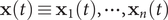 $ \mathbf{x}(t)\equiv {\mathbf{x}}_1(t),\cdots, {\mathbf{x}}_n(t) $
, and a transformation
$ \mathbf{x}(t)\equiv {\mathbf{x}}_1(t),\cdots, {\mathbf{x}}_n(t) $
, and a transformation
 $ \mathbf{s}(t) $
of
$ \mathbf{s}(t) $
of
 $ m $
component, namely
$ m $
component, namely
 $ \mathbf{s}(t)\equiv {s}_1\left(\mathbf{x}(t)\right),\cdots, {s}_m\left(\mathbf{x}(t)\right) $
. These transformations can be choice functions mapping to a single component of a coordinate such as
$ \mathbf{s}(t)\equiv {s}_1\left(\mathbf{x}(t)\right),\cdots, {s}_m\left(\mathbf{x}(t)\right) $
. These transformations can be choice functions mapping to a single component of a coordinate such as
 $ {s}_1(t)\equiv {x}_{1x}(t) $
, or some nonlinear functions mapping atomic coordinates to internal variables like dihedral angles, as long as the derivatives
$ {s}_1(t)\equiv {x}_{1x}(t) $
, or some nonlinear functions mapping atomic coordinates to internal variables like dihedral angles, as long as the derivatives
 $ {\mathrm{\nabla}}_{\mathbf{x}}\mathbf{s} $
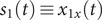
are well defined. An AE (Hinton and Salakhutdinov, Reference Hinton and Salakhutdinov2006; Goodfellow et al., Reference Goodfellow, Bengio and Courville2016), as illustrated in
Fig. 1a, can be regarded as a multilayer NN, which consists of an encoder part and a decoder part. In previous work employing AEs in CV discovery (Chen and Ferguson, Reference Chen and Ferguson2018; Chen et al., Reference Chen, Tan and Ferguson2018; Belkacemi et al., Reference Belkacemi, Gkeka, Lelièvre and Stoltz2022; Chen and Chipot, Reference Chen and Chipot2022), the inputs of the encoder are
$ {\mathrm{\nabla}}_{\mathbf{x}}\mathbf{s} $
are well defined. An AE (Hinton and Salakhutdinov, Reference Hinton and Salakhutdinov2006; Goodfellow et al., Reference Goodfellow, Bengio and Courville2016), as illustrated in
Fig. 1a, can be regarded as a multilayer NN, which consists of an encoder part and a decoder part. In previous work employing AEs in CV discovery (Chen and Ferguson, Reference Chen and Ferguson2018; Chen et al., Reference Chen, Tan and Ferguson2018; Belkacemi et al., Reference Belkacemi, Gkeka, Lelièvre and Stoltz2022; Chen and Chipot, Reference Chen and Chipot2022), the inputs of the encoder are
 $ \mathbf{s}(t) $
, and the encoder transforms them into a vector of latent variables
$ \mathbf{s}(t) $
, and the encoder transforms them into a vector of latent variables
 $ \boldsymbol{\xi} \equiv {\xi}_1,\cdots, {\xi}_d $
, which are then decoded into
$ \boldsymbol{\xi} \equiv {\xi}_1,\cdots, {\xi}_d $
, which are then decoded into
 $ \hat{\mathbf{s}}(t) $
by the decoder. In general, for the purpose of dimensionality reduction,
$ \hat{\mathbf{s}}(t) $
by the decoder. In general, for the purpose of dimensionality reduction,
 $ d $
is much smaller than
$ d $
is much smaller than
 $ m $
. A typical loss function – that is, a real-valued function for measuring the performance of a NN,
$ m $
. A typical loss function – that is, a real-valued function for measuring the performance of a NN,
 $ \mathrm{\mathcal{L}} $
, is equal for the classical AEs to the mean-squared-error (MSE), namely,
$ \mathrm{\mathcal{L}} $
, is equal for the classical AEs to the mean-squared-error (MSE), namely,
 $$ \mathrm{\mathcal{L}}=\frac{1}{N}\sum \limits_{j=0}^N{\Vert \mathbf{s}(j\Delta t)-\hat{\mathbf{s}}(j\Delta t)\Vert}^2, $$
where
 $ \Delta t $
is the time interval for discretizing and saving the trajectory, and
$ \Delta t $
is the time interval for discretizing and saving the trajectory, and
 $ N $
is the number of frames of the trajectory. It ought to be noted that since PCA can be interpreted as finding directions for projecting the data sets that either maximise the variance or minimise the reconstruction error, an AE that uses linear activation functions for all layers and MSE loss can strictly speaking be approximated to PCA. Nonlinear AEs resting on nonlinear activation functions can be regarded as a generalisation of PCA. Methods based on classical AEs have been applied to explore the conformational changes of chignolin (Belkacemi et al., Reference Belkacemi, Gkeka, Lelièvre and Stoltz2022) and Trp–cage (Chen and Ferguson, Reference Chen and Ferguson2018), to analyse the dynamic allostery triggered by ligand binding or mutagenesis (Tsuchiya et al., Reference Tsuchiya, Taneishi and Yonezawa2019), christo decode the conformational heterogeneities underlying the cytochrome P450 protein (Bandyopadhyay and Mondal, Reference Bandyopadhyay and Mondal2021), and to cluster the folded states of the
$ N $
is the number of frames of the trajectory. It ought to be noted that since PCA can be interpreted as finding directions for projecting the data sets that either maximise the variance or minimise the reconstruction error, an AE that uses linear activation functions for all layers and MSE loss can strictly speaking be approximated to PCA. Nonlinear AEs resting on nonlinear activation functions can be regarded as a generalisation of PCA. Methods based on classical AEs have been applied to explore the conformational changes of chignolin (Belkacemi et al., Reference Belkacemi, Gkeka, Lelièvre and Stoltz2022) and Trp–cage (Chen and Ferguson, Reference Chen and Ferguson2018), to analyse the dynamic allostery triggered by ligand binding or mutagenesis (Tsuchiya et al., Reference Tsuchiya, Taneishi and Yonezawa2019), christo decode the conformational heterogeneities underlying the cytochrome P450 protein (Bandyopadhyay and Mondal, Reference Bandyopadhyay and Mondal2021), and to cluster the folded states of the
 $ \beta \beta \alpha $
–protein (Ghorbani et al., Reference Ghorbani, Prasad, Klauda and Brooks2021).
$ \beta \beta \alpha $
–protein (Ghorbani et al., Reference Ghorbani, Prasad, Klauda and Brooks2021).
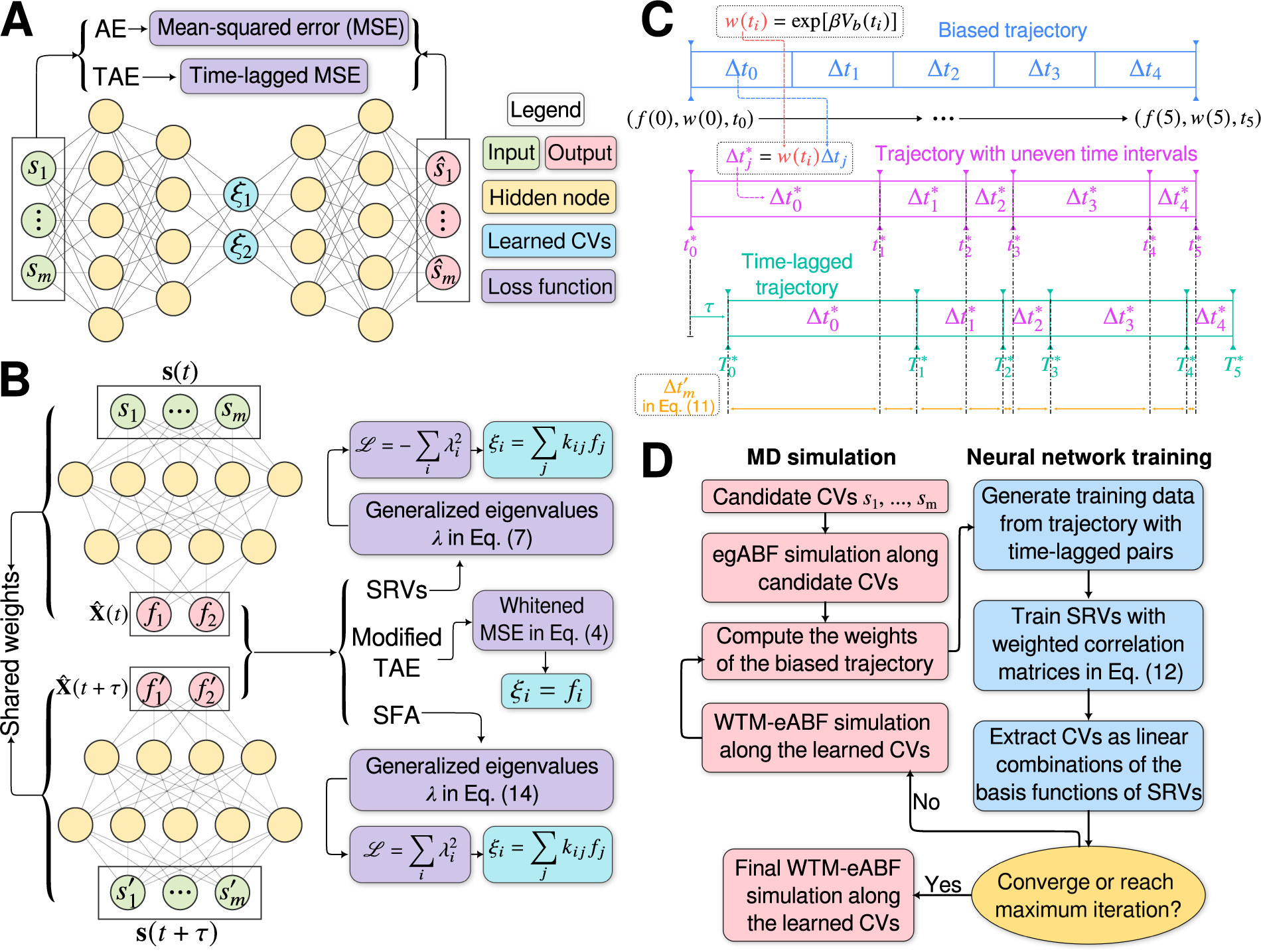
Fig. 1. (a) Schematic representation of a neural network used in an autoencoder (AE), or in a time-lagged autoencoder (TAE). (b) Schematic representation of a Siamese neural network used in modified TAEs, in state-free reversible VAMPnets (SRVs), and in a slow feature analysis (SFA). (c) Calculation of the reweighting factor
 $ \Delta {t}_m^{\prime } $
in Eq. (11). (d) Workflow employed in this work of data-driven collective-variable (CV) discovery from biased molecular dynamics (MD) simulations.
$ \Delta {t}_m^{\prime } $
in Eq. (11). (d) Workflow employed in this work of data-driven collective-variable (CV) discovery from biased molecular dynamics (MD) simulations.
Time-lagged AEs
The slow modes of molecular dynamics (MD) trajectories could be identified by exploiting their Markovianity and modelling the dynamics by means of a master equation (Mezić, Reference Mezić2005; Mitsutake et al., Reference Mitsutake, Iijima and Takano2011; Noé and Nüske, Reference Noé and Nüske2013; Husic and Pande, Reference Husic and Pande2018). From this perspective, various efforts have underscored that the slow modes can be expressed as the eigenfunctions of the Markov transition-rate matrix – or operator, and finding these eigenfunctions is tantamount to maximising the following functional in a variational principle sense (Takano and Miyashita, Reference Takano and Miyashita1995; Noé and Nüske, Reference Noé and Nüske2013):
 $$ R\left[{f}_{\theta}\right]=\frac{\left\langle {f}_{\theta}\left(\mathbf{x}(t)\right){f}_{\theta}\left(\mathbf{x}\left(t+\tau \right)\right)\right\rangle }{\left\langle {f}_{\theta}\left(\mathbf{x}(t)\right){f}_{\theta}\left(\mathbf{x}(t)\right)\right\rangle }, $$
where
 $ {f}_{\theta } $
are the eigenfunctions, and
$ {f}_{\theta } $
are the eigenfunctions, and
 $ \tau $
is the time lag. From a different point of view, Eq. (2) can be regarded as a normalised autocorrelation function, and the discovery of slow modes can be done by maximising it (Schwantes and Pande, Reference Schwantes and Pande2013). McGibbon et al. (Reference McGibbon, Husic and Pande2017) showed that the second leading eigenfunction of the transfer operator could be used as an appropriate CV – which they term a natural reaction coordinate since it is the most slowly decorrelating mode and maximally predictive of future evolution (Sultan and Pande, Reference Sultan and Pande2017). Akin to the relationship between PCA and AEs, maximisation of the correlation function in Eq. (2) can be approximated as the minimization of reconstruction loss between
$ \tau $
is the time lag. From a different point of view, Eq. (2) can be regarded as a normalised autocorrelation function, and the discovery of slow modes can be done by maximising it (Schwantes and Pande, Reference Schwantes and Pande2013). McGibbon et al. (Reference McGibbon, Husic and Pande2017) showed that the second leading eigenfunction of the transfer operator could be used as an appropriate CV – which they term a natural reaction coordinate since it is the most slowly decorrelating mode and maximally predictive of future evolution (Sultan and Pande, Reference Sultan and Pande2017). Akin to the relationship between PCA and AEs, maximisation of the correlation function in Eq. (2) can be approximated as the minimization of reconstruction loss between
 $ {f}_{\theta}\left(\mathbf{x}(t)\right) $
and
$ {f}_{\theta}\left(\mathbf{x}(t)\right) $
and
 $ {f}_{\theta}\left(\mathbf{x}\left(t+\tau \right)\right) $
by means of a regression approach, which leads to a TAE (Wehmeyer and Noé, Reference Wehmeyer and Noé2018). In other words, assuming the time lag
$ {f}_{\theta}\left(\mathbf{x}\left(t+\tau \right)\right) $
by means of a regression approach, which leads to a TAE (Wehmeyer and Noé, Reference Wehmeyer and Noé2018). In other words, assuming the time lag
 $ \tau $
can be discretized as
$ \tau $
can be discretized as
 $ \alpha \Delta t $
, and
$ \alpha \Delta t $
, and
 $ \mathbf{s}(t) $
is whitened (Kessy et al., Reference Kessy, Lewin and Strimmer2018) by zero-phase components analysis (Bell and Sejnowski, Reference Bell and Sejnowski1997), the loss function in TAEs is:
$ \mathbf{s}(t) $
is whitened (Kessy et al., Reference Kessy, Lewin and Strimmer2018) by zero-phase components analysis (Bell and Sejnowski, Reference Bell and Sejnowski1997), the loss function in TAEs is:
 $$ \mathrm{\mathcal{L}}=\frac{1}{N-\alpha}\sum \limits_{j=0}^{N-\alpha }{\Vert \mathbf{s}(j\Delta t+\alpha \Delta t)-\hat{\mathbf{s}}(j\Delta t)\Vert}^2. $$
TAEs can be considered as NN-based extensions (see Fig. 1a) to the dynamical mode decomposition (DMD) (Schmid, Reference Schmid2010) and time-lagged canonical correlation analysis (TCCA) (Hotelling, Reference Hotelling1936). TAEs have been successfully applied to study the conformational changes of villin (Wehmeyer and Noé, Reference Wehmeyer and Noé2018), and its extension by variational AE (Hernández et al., Reference Hernández, Wayment-Steele, Sultan, Husic and Pande2018) has been employed to train transferable CVs between one protein and its mutants (Sultan et al., Reference Sultan, Wayment-Steele and Pande2018).
Modified TAEs
Chen et al. (Reference Chen, Sidky and Ferguson2019a) revealed that TAEs with nonlinear activation functions tend to learn a mixture of slow modes, as well as the maximum-variance mode, and in some cases the slowest mode could be missing, leading to suboptimal CVs. To overcome this limitation, they proposed a modified TAE in the same work, which uses similar Siamese NNs (see Fig. 1b) as VAMPnets (Mardt et al., Reference Mardt, Pasquali, Wu and Noé2018), alongside its state-free reversible variant (Chen et al., Reference Chen, Sidky and Ferguson2019b). The loss function of modified TAEs is
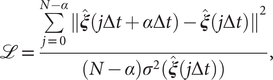 $$ \mathrm{\mathcal{L}}=\frac{\sum \limits_{j=0}^{N-\alpha }{\Vert \hat{\boldsymbol{\xi}}(j\Delta t+\alpha \Delta t)-\hat{\boldsymbol{\xi}}(j\Delta t)\Vert}^2}{(N-\alpha ){\sigma}^2(\hat{\boldsymbol{\xi}}(j\Delta t))}, $$
where the
 $ {\sigma}^2\left(\hat{\boldsymbol{\xi}}\left(j\Delta t\right)\right) $
is the variance of the encoder output. In addition, Chen et al. (Reference Chen, Sidky and Ferguson2019a) also showed that for those cases where
$ {\sigma}^2\left(\hat{\boldsymbol{\xi}}\left(j\Delta t\right)\right) $
is the variance of the encoder output. In addition, Chen et al. (Reference Chen, Sidky and Ferguson2019a) also showed that for those cases where
 $ m=1 $
, the modified TAEs are equivalent to the SRVs (Chen et al., Reference Chen, Sidky and Ferguson2019b), albeit the latter can guarantee the orthogonality of the latent variables by employing a variational approach in Eq. (2) with an eigendecomposition, as will be discussed in the following section.
$ m=1 $
, the modified TAEs are equivalent to the SRVs (Chen et al., Reference Chen, Sidky and Ferguson2019b), albeit the latter can guarantee the orthogonality of the latent variables by employing a variational approach in Eq. (2) with an eigendecomposition, as will be discussed in the following section.
VAMPnets and its state-free reversible derivative
VAMPnets (Mardt et al., Reference Mardt, Pasquali, Wu and Noé2018) employ the same Siamese NN (Bromley et al., Reference Bromley, Bentz, Bottou, Guyon, Lecun, Moore, Säckinger and Shah1993; Chicco, Reference Chicco and Cartwright2021) (see
Fig. 1b) as discussed previously, but instead of turning to the regression approach of Eq. (3), they solve the variational problem in Eq. (2) by employing TCCA on the encoded features. Assuming that the encoder can be expressed as a zero-mean multivariate basis function,
 $ \mathbf{f}\left(\mathbf{s}(t)\right) $
, the loss function of VAMPnets is,
$ \mathbf{f}\left(\mathbf{s}(t)\right) $
, the loss function of VAMPnets is,
 $$ \mathrm{\mathcal{L}}={\Vert \mathbf{C}{(t,t)}^{-\frac{1}{2}}\mathbf{C}(t,t+\tau )\mathbf{C}(t+\tau, t+\tau ){}^{-\frac{1}{2}}\Vert}_F^2, $$
where
 $ {\left\Vert \cdot \right\Vert}_F $
denotes the Frobenius norm of a matrix, and the correlation matrices
$ {\left\Vert \cdot \right\Vert}_F $
denotes the Frobenius norm of a matrix, and the correlation matrices
 $ \mathbf{C}\left(t,t\right) $
,
$ \mathbf{C}\left(t,t\right) $
,
 $ \mathbf{C}\left(t,t+\tau \right) $
and
$ \mathbf{C}\left(t,t+\tau \right) $
and
 $ \mathbf{C}\left(t+\tau, t+\tau \right) $
(Wu and Noé, Reference Wu and Noé2020) are defined, respectively, as:
$ \mathbf{C}\left(t+\tau, t+\tau \right) $
(Wu and Noé, Reference Wu and Noé2020) are defined, respectively, as:
 $$ \left\{\begin{array}{ll}\mathbf{C}\left(t,t\right)& =\frac{1}{N-\alpha}\hat{\mathbf{X}}(t)\hat{\mathbf{X}}{(t)}^{\mathrm{T}}\\ {}\mathbf{C}\left(t,t+\tau \right)& =\frac{1}{N-\alpha}\hat{\mathbf{X}}(t)\hat{\mathbf{X}}{\left(t+\tau \right)}^{\mathrm{T}}\\ {}\mathbf{C}\left(t+\tau, t+\tau \right)& =\frac{1}{N-\alpha}\hat{\mathbf{X}}\left(t+\tau \right)\hat{\mathbf{X}}{\left(t+\tau \right)}^{\mathrm{T}},\end{array}\right. $$
where the elements in
 $ \hat{\mathbf{X}}(t) $
and
$ \hat{\mathbf{X}}(t) $
and
 $ \hat{\mathbf{X}}\left(t+\tau \right) $
are
$ \hat{\mathbf{X}}\left(t+\tau \right) $
are
 $ {\hat{X}}_{ij}(t)={f}_i\left(\mathbf{s}\left(j\Delta t\right)\right) $
and
$ {\hat{X}}_{ij}(t)={f}_i\left(\mathbf{s}\left(j\Delta t\right)\right) $
and
 $ {\hat{X}}_{ij}\left(t+\tau \right)={f}_i\left(\mathbf{s}\left(j\Delta t+\alpha \Delta t\right)\right) $
, respectively. If the dynamics are reversible, which is the case in equilibrium MD simulations, the loss function relates to the eigenvalues of the Koopman operator of the Markov process by
$ {\hat{X}}_{ij}\left(t+\tau \right)={f}_i\left(\mathbf{s}\left(j\Delta t+\alpha \Delta t\right)\right) $
, respectively. If the dynamics are reversible, which is the case in equilibrium MD simulations, the loss function relates to the eigenvalues of the Koopman operator of the Markov process by
 $ \mathrm{\mathcal{L}}=-\sum \limits_{i=1}^m{\lambda}_i^2 $
, where
$ \mathrm{\mathcal{L}}=-\sum \limits_{i=1}^m{\lambda}_i^2 $
, where
 $ {\lambda}_i $
is the eigenvalues solved from the following generalised eigenvalue problem (Schwantes and Pande, Reference Schwantes and Pande2013):
$ {\lambda}_i $
is the eigenvalues solved from the following generalised eigenvalue problem (Schwantes and Pande, Reference Schwantes and Pande2013):
 $$ \mathbf{C}\left(t,t+\tau \right)\mathbf{V}=\mathbf{C}\left(t,t\right)\mathbf{V}\boldsymbol{\Lambda } . $$
Here,
 $ \boldsymbol{\Lambda} $
is
$ \boldsymbol{\Lambda} $
is
 $ \operatorname{diag}\left({\lambda}_1,\cdots, {\lambda}_m\right) $
, and
$ \operatorname{diag}\left({\lambda}_1,\cdots, {\lambda}_m\right) $
, and
 $ \mathbf{V} $
is a matrix containing the eigenvectors. The optimization of the loss function can be regarded as maximising the total kinetic variance (Noé and Clementi, Reference Noé and Clementi2015). After optimization, the learned CVs can be obtained by linear combinations of the components of
$ \mathbf{V} $
is a matrix containing the eigenvectors. The optimization of the loss function can be regarded as maximising the total kinetic variance (Noé and Clementi, Reference Noé and Clementi2015). After optimization, the learned CVs can be obtained by linear combinations of the components of
 $ \mathbf{f} $
, with the weights from the eigenvectors, namely
$ \mathbf{f} $
, with the weights from the eigenvectors, namely
 $ {\xi}_i={\sum}_j{k}_{ij}{f}_j $
, where
$ {\xi}_i={\sum}_j{k}_{ij}{f}_j $
, where
 $ {k}_{ij} $
is the -
$ {k}_{ij} $
is the -
 $ j $
th component of the -
$ j $
th component of the -
 $ i $
th column vector of
$ i $
th column vector of
 $ \mathbf{V} $
. The number of learned CVs should not be greater than the number of components of
$ \mathbf{V} $
. The number of learned CVs should not be greater than the number of components of
 $ \mathbf{f} $
. The use of Eq. (7) with basis function
$ \mathbf{f} $
. The use of Eq. (7) with basis function
 $ \mathbf{f} $
can be viewed as an extension of tICA (Naritomi and Fuchigami, Reference Naritomi and Fuchigami2011), with a kernel function (Schwantes and Pande, Reference Schwantes and Pande2015), while the kernel functions are approximated by the NNs. This loss function is also employed by both SRVs (Chen et al., Reference Chen, Sidky and Ferguson2019b) and deep-TICA (Bonati et al., Reference Bonati, Piccini and Parrinello2021). It ought to be noted that while the principle of Eqs. (6) and (7) is generally considered to have been proposed as early as 1994 by Molgedey and Schuster (Reference Molgedey and Schuster1994), a similar methodology has been devised independently in many other fields under different names, such as relaxation mode analysis (Takano and Miyashita, Reference Takano and Miyashita1995; Mitsutake et al., Reference Mitsutake, Iijima and Takano2011), second-order independent component analysis (Belouchrani et al., Reference Belouchrani, Abed-Meraim, Cardoso and Moulines1997), and temporal decorrelation source separation (Ziehe and Müller, Reference Ziehe, Müller, Niklasson, Bodén and Ziemke1998). VAMPnets have been utilised to find metastable states in the folding of the N-terminal domain of ribosomal protein L9 (NTL9) (Mardt et al., Reference Mardt, Pasquali, Wu and Noé2018), to determine a kinetic ensemble of the 42-amino-acid amyloid-
$ \mathbf{f} $
can be viewed as an extension of tICA (Naritomi and Fuchigami, Reference Naritomi and Fuchigami2011), with a kernel function (Schwantes and Pande, Reference Schwantes and Pande2015), while the kernel functions are approximated by the NNs. This loss function is also employed by both SRVs (Chen et al., Reference Chen, Sidky and Ferguson2019b) and deep-TICA (Bonati et al., Reference Bonati, Piccini and Parrinello2021). It ought to be noted that while the principle of Eqs. (6) and (7) is generally considered to have been proposed as early as 1994 by Molgedey and Schuster (Reference Molgedey and Schuster1994), a similar methodology has been devised independently in many other fields under different names, such as relaxation mode analysis (Takano and Miyashita, Reference Takano and Miyashita1995; Mitsutake et al., Reference Mitsutake, Iijima and Takano2011), second-order independent component analysis (Belouchrani et al., Reference Belouchrani, Abed-Meraim, Cardoso and Moulines1997), and temporal decorrelation source separation (Ziehe and Müller, Reference Ziehe, Müller, Niklasson, Bodén and Ziemke1998). VAMPnets have been utilised to find metastable states in the folding of the N-terminal domain of ribosomal protein L9 (NTL9) (Mardt et al., Reference Mardt, Pasquali, Wu and Noé2018), to determine a kinetic ensemble of the 42-amino-acid amyloid-
 $ \beta $
peptide (Löhr et al., Reference Löhr, Kohlhoff, Heller, Camilloni and Vendruscolo2021). In addition, its state-free reversible variant has been employed for identifying the metastable states of DNA hybridization/dehybridization (Jones et al., Reference Jones, Ashwood, Tokmakoff and Ferguson2021).
$ \beta $
peptide (Löhr et al., Reference Löhr, Kohlhoff, Heller, Camilloni and Vendruscolo2021). In addition, its state-free reversible variant has been employed for identifying the metastable states of DNA hybridization/dehybridization (Jones et al., Reference Jones, Ashwood, Tokmakoff and Ferguson2021).
Iterative learning with a biased trajectory
A common shortcoming of all data-driven dimensionality reduction methods is that the learned models may perform poorly on unseen data. To be specific, if the states of interest are not part of the training set, the learned CVs could lose the information about them. To address this difficulty, one can turn to an iterative learning strategy, that is, one can run the following iterations until some convergence criteria are met, namely, (a) feeding the model with an initial trajectory, (b) biasing the next round of the simulation with the learned CVs, and (c) using the biased trajectory to train the model again. This strategy has been employed in MESA (Chen and Ferguson, Reference Chen and Ferguson2018), FEBILAE (Belkacemi et al., Reference Belkacemi, Gkeka, Lelièvre and Stoltz2022), deep-TICA (Bonati et al., Reference Bonati, Piccini and Parrinello2021) and PIB (Wang et al., Reference Wang, Ribeiro and Tiwary2019). Specifically, in this contribution, we start by training the SRVs with an initial trajectory from extended generalised adaptive biasing force (egABF) (Zhao et al., Reference Zhao, Fu, Lelièvre, Shao, Chipot and Cai2017) simulations along candidate CVs chosen coarsely by physicochemical intuition – that is, educated guesses, and employ well-tempered meta-extended ABF (WTM-eABF) (Fu et al., Reference Fu, Shao, Cai and Chipot2019) simulations along the learned CVs in successive iterations, as depicted in Fig. 1d. A key issue of iterative learning is the reweighting of the biased trajectory, or in plain words, making the training from a short biased trajectory equivalent to that of a long unbiased trajectory. We summarise hereafter the alternate approaches for processing the biased trajectories.
No reweighting
Instead of reweighting, one can train an AE with the biased trajectory as is. This strategy is used in the MESA protocol (Chen et al., Reference Chen, Tan and Ferguson2018). With FEBILAE, it was shown, however, that ignoring the biases could introduce systematic errors (Belkacemi et al., Reference Belkacemi, Gkeka, Lelièvre and Stoltz2022).
Direct reweighting
Assuming that the biasing potential along
 $ \mathbf{s} $
,
$ \mathbf{s} $
,
 $ {V}_b\left(\mathbf{s}\right) $
, is suitably converged, then the unbiased time average of an observable
$ {V}_b\left(\mathbf{s}\right) $
, is suitably converged, then the unbiased time average of an observable
 $ {X}_t $
of the process of interest can be computed as
$ {X}_t $
of the process of interest can be computed as
 $$ \langle {X}_t\rangle =\frac{{\displaystyle {\int}_0^t{X}_t{e}^{\beta {V}_b({\mathbf{s}}_{\tau })}\mathrm{d}\tau }}{{\displaystyle {\int}_0^t{e}^{\beta {V}_b({\mathbf{s}}_{\tau })}\mathrm{d}\tau }}, $$
where
 $ \beta =1/{k}_{\mathrm{B}}T $
,
$ \beta =1/{k}_{\mathrm{B}}T $
,
 $ {k}_{\mathrm{B}} $
is the Boltzmann constant and
$ {k}_{\mathrm{B}} $
is the Boltzmann constant and
 $ T $
is the temperature of the simulation. Combining Eq. (8) with Eq. (1) yields the weighted MSE loss function, expressed as
$ T $
is the temperature of the simulation. Combining Eq. (8) with Eq. (1) yields the weighted MSE loss function, expressed as
 $$ {\mathrm{\mathcal{L}}}_w=\frac{\sum \limits_{j=0}^Nw(j\Delta t){\Vert \mathbf{s}(j\Delta t)-\hat{\mathbf{s}}(j\Delta t)\Vert}^2}{\sum \limits_{j=0}^Nw(j\Delta t)}, $$
where the weight for each time frame,
 $ w\left(j\Delta t\right) $
, is computed as
$ w\left(j\Delta t\right) $
, is computed as
 $ {e}^{\beta {V}_b\left(\mathbf{s}\left(j\Delta t\right)\right)} $
. Whereas this reweighting strategy is straightforward for classical AEs, and is utilised in FEBILAE (Belkacemi et al., Reference Belkacemi, Gkeka, Lelièvre and Stoltz2022), transposing it to TAEs, modified TAEs and VAMPnets is not obvious, since Eqs. (2), (3), (4) and (6) include correlations between two observable quantities that may carry different weights.
$ {e}^{\beta {V}_b\left(\mathbf{s}\left(j\Delta t\right)\right)} $
. Whereas this reweighting strategy is straightforward for classical AEs, and is utilised in FEBILAE (Belkacemi et al., Reference Belkacemi, Gkeka, Lelièvre and Stoltz2022), transposing it to TAEs, modified TAEs and VAMPnets is not obvious, since Eqs. (2), (3), (4) and (6) include correlations between two observable quantities that may carry different weights.
Reweighting by uneven time intervals
Yang and Parrinello (Reference Yang and Parrinello2018) developed a numerical scheme by treating the biased trajectory as an unevenly spaced time series. Under these premises, the calculation of the elements in
 $ \mathbf{C}\left(t,t+\tau \right) $
follows:
$ \mathbf{C}\left(t,t+\tau \right) $
follows:
 $$ {C}_{ik}\left(t,t+\tau \right)=\frac{\sum \limits_{j=0}^{N-\alpha}\Delta {t}_j{\hat{\xi}}_i\left(j\Delta t\right){\hat{\xi}}_k\left(j\Delta t+\alpha \Delta t\right)}{\sum \limits_{j=0}^{N-\alpha}\Delta {t}_j}, $$
and since the time intervals
 $ \Delta {t}_j $
in an unbiased trajectory are even, the overlapping time between frames
$ \Delta {t}_j $
in an unbiased trajectory are even, the overlapping time between frames
 $ j\Delta t $
and
$ j\Delta t $
and
 $ j\Delta t+\alpha \Delta t $
is the same for all time-lagged pairs. As a result, the
$ j\Delta t+\alpha \Delta t $
is the same for all time-lagged pairs. As a result, the
 $ \Delta t $
factors appearing in both the numerator and the denominator cancel out. In a biased trajectory, however,
$ \Delta t $
factors appearing in both the numerator and the denominator cancel out. In a biased trajectory, however,
 $ \Delta {t}_j $
may differ between any two frames. To reweight the time series, we first need to compute the unbiased time interval for each frame, namely
$ \Delta {t}_j $
may differ between any two frames. To reweight the time series, we first need to compute the unbiased time interval for each frame, namely
 $ \Delta {t}_j^{\ast }=\Delta {te}^{\beta {V}_b\left(\mathbf{s}\left(j\Delta t\right)\right)} $
(see also Eqs. (2)–(4) in Hamelberg et al., Reference Hamelberg, Mongan and McCammon2004), and then find the overlapping time for each time-lagged pairs
$ \Delta {t}_j^{\ast }=\Delta {te}^{\beta {V}_b\left(\mathbf{s}\left(j\Delta t\right)\right)} $
(see also Eqs. (2)–(4) in Hamelberg et al., Reference Hamelberg, Mongan and McCammon2004), and then find the overlapping time for each time-lagged pairs
 $ \boldsymbol{\xi} \left(j\Delta t\right) $
and
$ \boldsymbol{\xi} \left(j\Delta t\right) $
and
 $ \boldsymbol{\xi} \left(j\Delta t+\alpha \Delta t\right) $
by following the sequence of steps:
$ \boldsymbol{\xi} \left(j\Delta t+\alpha \Delta t\right) $
by following the sequence of steps:
-
(1) Compute the unbiased simulation time for each frame as a cumulative sum of
 $ \Delta {t}_j^{\ast } $
, namely,
$ {t}_j^{\ast }={\sum}_{l=0}^j\Delta {te}^{\beta {V}_b\left(\mathbf{s}\left(j\Delta t\right)\right)} $
;
$ \Delta {t}_j^{\ast } $
, namely,
$ {t}_j^{\ast }={\sum}_{l=0}^j\Delta {te}^{\beta {V}_b\left(\mathbf{s}\left(j\Delta t\right)\right)} $
; -
(2) Compute the unbiased lagged simulation time for each frame as
$ {T}_j^{\ast }={t}_j^{\ast }+\tau $
, where
$ \tau $
is the specified time lag; -
(3) Two monotonically increasing sequences
$ {S}_t=\left({t}_0^{\ast },\cdots, {t}_N^{\ast}\right) $
and
$ {S}_T=\left({T}_0^{\ast },\cdots, {T}_N^{\ast}\right) $
can be obtained from the previous steps. Now one can construct a union set of
$ {S}_t $
and
$ {S}_T $
with elements lying between
$ {T}_0^{\ast } $
and
$ {t}_N^{\ast } $
, namely,
$ {S}_u=\left\{{t}_j^{\prime}\in {S}_t\cup {S}_T|{t}_j^{\prime }>{T}_0^{\ast}\wedge {t}_j^{\prime }<{t}_N^{\ast}\right\} $
, and then sort
$ {S}_u $
by increasing order; -
(4) Assuming that
$ {S}_u $
has
$ M $
elements
$ {t}_1^{\prime },\cdots, {t}_M^{\prime } $
in increasing order, for each element
$ {t}_m^{\prime } $
, we can find an index
$ i $
such that
$ {t}_i^{\ast }<{t}_m^{\prime }<{t}_{i+1}^{\ast } $
, and also an index
$ j $
such that
$ {T}_i^{\ast }<{t}_m^{\prime }<{T}_{i+1}^{\ast } $
. Since the finding of indices can be viewed as mappings or functions, then we obtain a list
$ L $
with
$ M-1 $
elements including all triplets
$ \left\{f(m),g(m),\Delta {t}_m^{\prime}\right\} $
, where
$ f(m)=i,\hskip0.2em g(m)=j $
and
$ \Delta {t}_m^{\prime }={t}_{m+1}^{\prime }-{t}_m^{\prime } $
(see
Fig. 1c for a schematized representation of the
$ \Delta {t}_m^{\prime } $
calculation); -
(5) The reweighted correlation function can be calculated as:
(11)
$$ {C}_{ik}\left(t,t+\tau \right)=\frac{\sum \limits_{m=1}^{M-1}\Delta {t}_m^{\prime }{\hat{\xi}}_i\left(f(m)\right){\hat{\xi}}_k\left(g(m)\right)}{\sum \limits_{m=1}^{M-1}\Delta {t}_m^{\prime }}. $$


Koopman reweighting
Wu et al. (Reference Wu, Nüske, Paul, Klus, Koltai and Noé2017) proposed an approximation of the weighted correlation by means of Koopman reweighting, namely,
 $$ {C}_{ik}\left(t,t+\tau \right)\approx \frac{\sum \limits_{j=0}^{N-\alpha }w\left(j\Delta t\right){\hat{\xi}}_i\left(j\Delta t\right){\hat{\xi}}_k\left(j\Delta t+\alpha \Delta t\right)}{\sum \limits_{j=0}^{N-\alpha }w\left(j\Delta t\right)}. $$
In contrast with Eq. (11), Eq. (12) uses only the weight of time frame
 $ j\Delta t $
. This strategy has been used by McCarty and Parrinello (Reference McCarty and Parrinello2017) for improving the selection of CVs with tICA. To determine a suitable reweighting strategy for the iterative learning, we compare the accuracy of Eqs. (11) and (12) for reweighting in numerical examples, as will be discussed in the following section.
$ j\Delta t $
. This strategy has been used by McCarty and Parrinello (Reference McCarty and Parrinello2017) for improving the selection of CVs with tICA. To determine a suitable reweighting strategy for the iterative learning, we compare the accuracy of Eqs. (11) and (12) for reweighting in numerical examples, as will be discussed in the following section.
Results and discussion
In this section, we discuss through a series of numerical examples the limitation of AEs for learning slow modes, and how to introduce temporal information could address this limitation. Next, we review the possible shortcoming of using nonlinear activation functions in TAEs, and show how it can be dealt with, turning to either SRVs or an extension of modified TAEs. In addition, we assess different reweighting schemes consistent with SRVs and biased trajectories, thereby paving the way for iterative learning with CV-based enhanced sampling. Next, we illustrate our protocol in the discovery of CVs of two prototypical biological processes, namely the isomerization of NANMA and trialanine. Finally, we reveal the potential connection between the temporal models investigated herein with the committor probability (Geissler et al., Reference Geissler, Dellago and Chandler1999) employed in transition path theory (Weinan and Vanden-Eijnden, Reference Weinan and Vanden-Eijnden2010).
AEs discover the high-variance modes instead of the slow modes
To illustrate the intrinsic limitations of classical AEs for capturing the most dominant features, we compared them and TAEs to learn a one-dimensional CV from overdamped Langevin dynamics trajectories with the following two-dimensional triple-well potential, using
 $ X $
and
$ X $
and
 $ Y $
as the input features for NNs, setting
$ Y $
as the input features for NNs, setting
 $ \alpha $
to 1.0 and to 10.0,
$ \alpha $
to 1.0 and to 10.0,
 $$ {\displaystyle \begin{array}{l}V\left(X,Y\right)=3{\mathrm{e}}^{-{X}^2}\left({\mathrm{e}}^{-{\left(Y-\frac{1}{3}\right)}^2/\alpha }-{\mathrm{e}}^{-{\left(Y-\frac{5}{3}\right)}^2/\alpha}\right)\\ {}\hskip7em -5{\mathrm{e}}^{-{Y}^2/\alpha}\left({\mathrm{e}}^{-{\left(X-1\right)}^2}+{\mathrm{e}}^{-{\left(X+1\right)}^2}\right)\\ {}\hskip7em +0.2{X}^4+0.2{\left(Y-\frac{1}{3}\right)}^4/{\alpha}^2.\end{array}} $$
The unit of variables
 $ X $
and
$ X $
and
 $ Y $
is angstrom, and the unit of the output of
$ Y $
is angstrom, and the unit of the output of
 $ V\left(X,Y\right) $
is kcal mol−1. The corresponding potential energy surfaces and the time evolution of the variables are shown in
Fig. 2a,
b,
e,
f. It can be easily deduced from
Fig. 2a,
e that for both
$ V\left(X,Y\right) $
is kcal mol−1. The corresponding potential energy surfaces and the time evolution of the variables are shown in
Fig. 2a,
b,
e,
f. It can be easily deduced from
Fig. 2a,
e that for both
 $ \alpha = $
1.0 and
$ \alpha = $
1.0 and
 $ \alpha = $
10.0, the important DOF should be
$ \alpha = $
10.0, the important DOF should be
 $ X $
. As depicted in
Fig. 2c,
g, when training the trajectories by AEs, the value of the bottleneck layer,
$ X $
. As depicted in
Fig. 2c,
g, when training the trajectories by AEs, the value of the bottleneck layer,
 $ \xi $
, varies along
$ \xi $
, varies along
 $ X $
if
$ X $
if
 $ \alpha $
is 1.0, but switches to vary along
$ \alpha $
is 1.0, but switches to vary along
 $ Y $
if
$ Y $
if
 $ \alpha $
increases to 10.0. This seemingly surprising result indicates that AEs erroneously learn two distinct important DOFs, when there should be only one along
$ \alpha $
increases to 10.0. This seemingly surprising result indicates that AEs erroneously learn two distinct important DOFs, when there should be only one along
 $ X $
. In stark contrast, TAEs behave consistently for both
$ X $
. In stark contrast, TAEs behave consistently for both
 $ \alpha = $
1.0 (
Fig. 2d) and
$ \alpha = $
1.0 (
Fig. 2d) and
 $ \alpha = $
10.0 (
Fig. 2h), and the learned variable highly correlates with the movement along
$ \alpha = $
10.0 (
Fig. 2h), and the learned variable highly correlates with the movement along
 $ X $
, which is also the most dominant mode. The projections of the one-dimensional learned variable onto
$ X $
, which is also the most dominant mode. The projections of the one-dimensional learned variable onto
 $ X $
and
$ X $
and
 $ Y $
of other models discussed in this contribution are shown in Supplementary Fig. 1. It can be rationalised by the fact that AEs actually learn the variables that correspond to the highest variance, which is, indeed, reflected in our analyses, with a variance for
$ Y $
of other models discussed in this contribution are shown in Supplementary Fig. 1. It can be rationalised by the fact that AEs actually learn the variables that correspond to the highest variance, which is, indeed, reflected in our analyses, with a variance for
 $ X(t) $
of 1.0, greater than that for
$ X(t) $
of 1.0, greater than that for
 $ Y(t) $
, equal to 0.18, when
$ Y(t) $
, equal to 0.18, when
 $ \alpha = $
1.0. Conversely, when
$ \alpha = $
1.0. Conversely, when
 $ \alpha = $
10.0, the variance for
$ \alpha = $
10.0, the variance for
 $ X(t) $
is 0.78, smaller than that of
$ X(t) $
is 0.78, smaller than that of
 $ Y(t) $
, equal to 0.99. This discrepancy in the variances may also explain why AE fails to encode the correct important DOF when
$ Y(t) $
, equal to 0.99. This discrepancy in the variances may also explain why AE fails to encode the correct important DOF when
 $ \alpha = $
10.0. The present comparison underscores that it is crucial to introduce temporal information into the models for learning the slow modes, as opposed to the high-variance ones. Nevertheless, as discussed in a recent review of Markov state models, sometimes slow modes may still not coincide with the important DOFs that are sought (Husic and Pande, Reference Husic and Pande2018). We, therefore, need to select proper candidate CVs, or features, as the learning input, and that is why we advocate here to combine data-driven and intuition-based approaches.
$ \alpha = $
10.0. The present comparison underscores that it is crucial to introduce temporal information into the models for learning the slow modes, as opposed to the high-variance ones. Nevertheless, as discussed in a recent review of Markov state models, sometimes slow modes may still not coincide with the important DOFs that are sought (Husic and Pande, Reference Husic and Pande2018). We, therefore, need to select proper candidate CVs, or features, as the learning input, and that is why we advocate here to combine data-driven and intuition-based approaches.
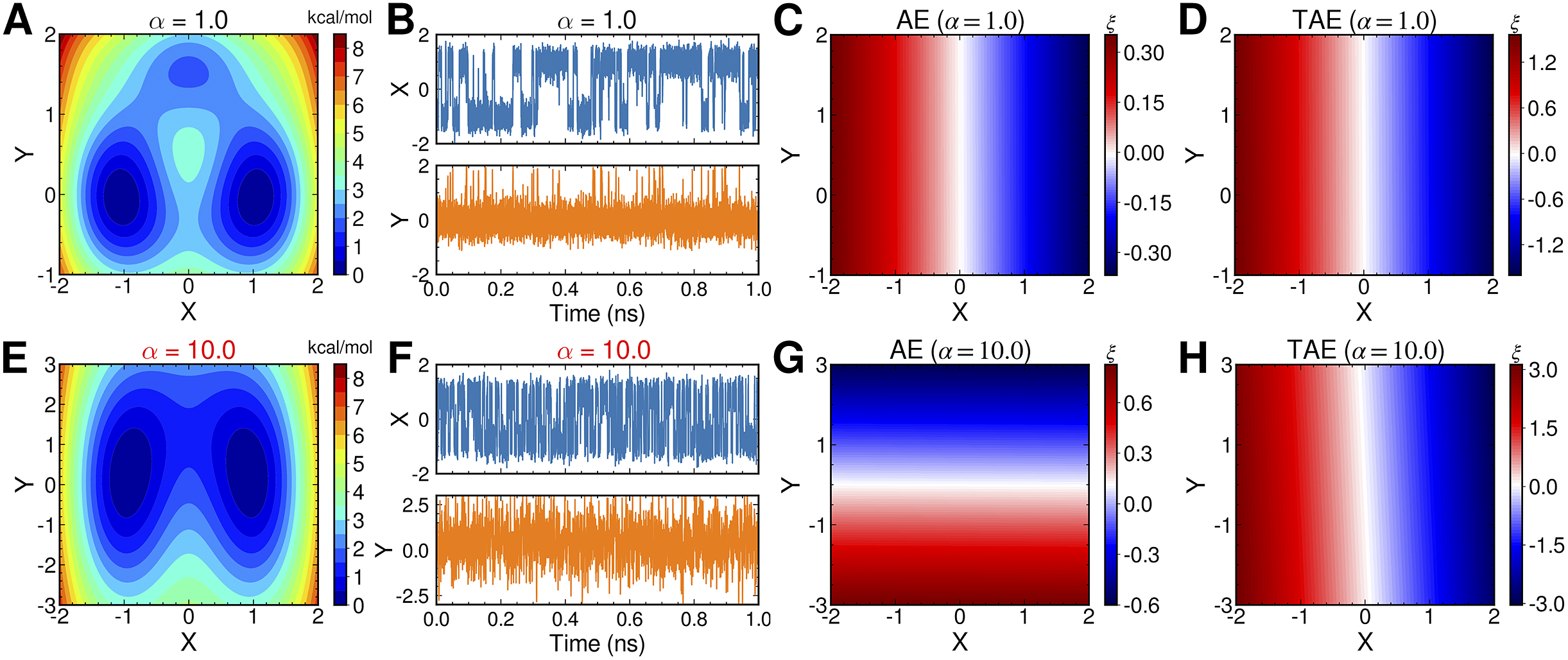
Fig. 2. Potential energy surfaces of
 $ V(X,Y) $
with (a) α = 1.0 and (e) α = 10.0; Time evolution of X and Y when (b) α = 1.0 and (f) α = 10.0; Projections of the encoded variable
$ V(X,Y) $
with (a) α = 1.0 and (e) α = 10.0; Time evolution of X and Y when (b) α = 1.0 and (f) α = 10.0; Projections of the encoded variable
 $ \xi $
on X and Y from AEs training with trajectories of (c) α = 1.0 and (g) α = 10.0; Projections of the encoded variable
$ \xi $
on X and Y from AEs training with trajectories of (c) α = 1.0 and (g) α = 10.0; Projections of the encoded variable
 $ \xi $
on X and Y from TAEs training with trajectories of (d) α = 1.0 and (h) α = 10.0.
$ \xi $
on X and Y from TAEs training with trajectories of (d) α = 1.0 and (h) α = 10.0.
Both nonlinear modified TAE and SRVs can correctly learn the slow modes
Chen et al. (Reference Chen, Sidky and Ferguson2019a) have illustrated that nonlinear TAEs learn a mixture of slow modes and high-variance modes, and proposed the nonlinear modified TAEs that can learn correctly the slow modes, but comparing to SRVs, modified TAEs cannot generate orthogonal and multidimensional latent variables that are suitable for CV-based biased simulations. Here, we confirm their results numerically by using the potential depicted in
Fig. 2c, but we also propose that the modified TAE can be extended to slow feature analysis (SFA) (Wiskott and Sejnowski, Reference Wiskott and Sejnowski2002; Berkes and Wiskott, Reference Berkes and Wiskott2005; Song and Zhao, Reference Song and Zhao2022) (see
Fig. 1b), which can render the latent variables orthogonal in multidimensional cases, since Eq. (4) resembles the SFA loss function in the one-dimensional case. In an SFA, if the encoder,
 $ \mathbf{f} $
, is multivariate, Eq. (4) should be formulated as the following generalised eigenvalue problem:
$ \mathbf{f} $
, is multivariate, Eq. (4) should be formulated as the following generalised eigenvalue problem:
 $$ \Big\{\begin{array}{l}\mathbf{A}\hskip1em =\frac{1}{N-\alpha }[\hat{\mathbf{X}}(t+\tau )-\hat{\mathbf{X}}(t)]{[\hat{\mathbf{X}}(t+\tau )-\hat{\mathbf{X}}(t)]}^{\mathsf{T}}\\ {}\mathbf{A}\mathbf{V}=\mathbf{C}(t,t)\mathbf{V}\boldsymbol{\Lambda } .\end{array}\operatorname{} $$
The corresponding loss function is the sum of squared eigenvalues in Eq. (14), namely,
 $ \mathrm{\mathcal{L}}={\sum}_{i=1}^m{\lambda}_i^2 $
. Akin to SRVs, the CVs are then expressed as linear combinations of the components of
$ \mathrm{\mathcal{L}}={\sum}_{i=1}^m{\lambda}_i^2 $
. Akin to SRVs, the CVs are then expressed as linear combinations of the components of
 $ \mathbf{f} $
. We note that our use of SFA in conjunction with NNs is quite similar to the deep SFA (DSFA) for change detection in images (Du et al., Reference Du, Ru, Wu and Zhang2019), except that in our two encoders, the weights and biases are shared. At first glance, Eq. (14) looks similar to Eq. (7), and also the loss function of SFA resembles that of SRVs, except that the former does not have a negative sign. Indeed, in the linear case, the two methods have been proved to be equivalent (Blaschke et al., Reference Blaschke, Berkes and Wiskott2006; Wang and Zhao, Reference Wang and Zhao2020), but the relationship is not so clear in the nonlinear case, whereby a NN with nonlinear activation functions is employed to encode
$ \mathbf{f} $
. We note that our use of SFA in conjunction with NNs is quite similar to the deep SFA (DSFA) for change detection in images (Du et al., Reference Du, Ru, Wu and Zhang2019), except that in our two encoders, the weights and biases are shared. At first glance, Eq. (14) looks similar to Eq. (7), and also the loss function of SFA resembles that of SRVs, except that the former does not have a negative sign. Indeed, in the linear case, the two methods have been proved to be equivalent (Blaschke et al., Reference Blaschke, Berkes and Wiskott2006; Wang and Zhao, Reference Wang and Zhao2020), but the relationship is not so clear in the nonlinear case, whereby a NN with nonlinear activation functions is employed to encode
 $ \hat{\mathbf{X}} $
. Consequently, to investigate the performance of finding nonlinear latent variables for slow modes, in this section, we benchmark a TAE, modified TAE, SRVs and SFA using the unbiased trajectory generated from the potential energy function Eq. (13), with
$ \hat{\mathbf{X}} $
. Consequently, to investigate the performance of finding nonlinear latent variables for slow modes, in this section, we benchmark a TAE, modified TAE, SRVs and SFA using the unbiased trajectory generated from the potential energy function Eq. (13), with
 $ \alpha =10.0 $
. We used two hidden layers with hyperbolic tangent as the activation functions in both the encoder and the decoder part of TAEs, giving a final architecture of 2-40-40-
$ \alpha =10.0 $
. We used two hidden layers with hyperbolic tangent as the activation functions in both the encoder and the decoder part of TAEs, giving a final architecture of 2-40-40-
 $ n $
-40-40-2. The activation functions of the input, the bottleneck and the output layer are linear. Similarly, we used an architecture of 2-40-40-
$ n $
-40-40-2. The activation functions of the input, the bottleneck and the output layer are linear. Similarly, we used an architecture of 2-40-40-
 $ n $
for the other Siamese NNs (modified TAE, SFA and SRVs). We have tested both cases, where
$ n $
for the other Siamese NNs (modified TAE, SFA and SRVs). We have tested both cases, where
 $ n=1 $
and
$ n=1 $
and
 $ n=2 $
, and used a time lag of 0.02 ps.
$ n=2 $
, and used a time lag of 0.02 ps.
The projections of the encoded values in the one-dimensional case – that is, the outputs of the bottleneck layer in the TAE, the last layers in the modified TAE and the linear combinations of basis functions of SFA and SRVs – are gathered in
Fig. 3a–
d. In
Fig. 3a, we can clearly see that the latent variable of the TAE is split into the left and right sides along
 $ X $
, and on each side,
$ X $
, and on each side,
 $ \xi $
varies along
$ \xi $
varies along
 $ Y $
. This result implies that while the nonlinear TAE is able to learn a latent variable, distinguishing the two basins shown in
Fig. 2c, it is also affected by the high-variance mode in
$ Y $
. This result implies that while the nonlinear TAE is able to learn a latent variable, distinguishing the two basins shown in
Fig. 2c, it is also affected by the high-variance mode in
 $ Y $
. In stark contrast, the modified TAE, SFA and SRVs, with nonlinear activation functions, appropriately learn the slow modes, that is, the learned CV varies almost only along the transition between the two basins. In the two-dimensional case, comparing
Fig. 3f,
j, we note that the modified TAE learns two nearly identical modes, both varying along
$ Y $
. In stark contrast, the modified TAE, SFA and SRVs, with nonlinear activation functions, appropriately learn the slow modes, that is, the learned CV varies almost only along the transition between the two basins. In the two-dimensional case, comparing
Fig. 3f,
j, we note that the modified TAE learns two nearly identical modes, both varying along
 $ X $
. The generalisation of the modified TAE, using the SFA loss function embodied in Eq. (14), is, however, able to recognise two distinct, approximately orthogonal modes (see
Fig. 3g,
k), in line with the results of the SRVs (see
Fig. 3h,
l).
$ X $
. The generalisation of the modified TAE, using the SFA loss function embodied in Eq. (14), is, however, able to recognise two distinct, approximately orthogonal modes (see
Fig. 3g,
k), in line with the results of the SRVs (see
Fig. 3h,
l).

Fig. 3. Projections of the one-dimensional CV
 $ \xi $
learned from unbiased trajectories when
$ \xi $
learned from unbiased trajectories when
 $ \alpha =10.0 $
on X and Y of (a) TAE, (b) modified TAE, (c) SFA and (d) SRVs. Projections of the 2D CVs (
$ \alpha =10.0 $
on X and Y of (a) TAE, (b) modified TAE, (c) SFA and (d) SRVs. Projections of the 2D CVs (
 $ {\xi}_1 $
,
$ {\xi}_1 $
,
 $ {\xi}_2 $
) learned from unbiased trajectories when
$ {\xi}_2 $
) learned from unbiased trajectories when
 $ \alpha =10.0 $
on X and Y of (e,i) TAE, (f,j) modified TAE, (g,k) SFA and (h,l) SRVs. Projections of the 2D CVs (
$ \alpha =10.0 $
on X and Y of (e,i) TAE, (f,j) modified TAE, (g,k) SFA and (h,l) SRVs. Projections of the 2D CVs (
 $ {\xi}_1 $
,
$ {\xi}_1 $
,
 $ {\xi}_2 $
) learned by SRVs from an unbiased trajectory when
$ {\xi}_2 $
) learned by SRVs from an unbiased trajectory when
 $ \alpha =10.0 $
(m,n), from an egABF biased trajectory reweighted by Eq. (11) (o,p), and from an egABF biased trajectory reweighted by Eq. (12) (q,r).
$ \alpha =10.0 $
(m,n), from an egABF biased trajectory reweighted by Eq. (11) (o,p), and from an egABF biased trajectory reweighted by Eq. (12) (q,r).
Furthermore, we compared the two reweighting schemes, namely reweighting by uneven time intervals (Eq. (11)) and Koopman reweighting (Eq. (12)), for the calculation of the weighted correlation in SRVs from an egABF biased trajectory, with
 $ \alpha =1.0 $
. The variations of the two learned CVs,
$ \alpha =1.0 $
. The variations of the two learned CVs,
 $ {\xi}_1 $
(
Fig. 3q) and
$ {\xi}_1 $
(
Fig. 3q) and
 $ {\xi}_2 $
(
Fig. 3r), using Koopman reweighting, closely correlate with the reference ones (
Fig. 3m,
n) obtained from an unbiased trajectory. The results from the reweighting strategy with uneven time intervals (see
Fig. 3o,
p) clearly depart from the reference ones. Hence, we chose the Koopman reweighting scheme for learning CVs from biased simulations in our iterative approach. The accuracy of the scheme leaning on uneven time intervals for the evaluation of the correlations may, nevertheless, be improved by means of interpolations, either explicitly or implicitly via Fourier transform (Scargle, Reference Scargle1989), which falls beyond the scope of the present contribution.
$ {\xi}_2 $
(
Fig. 3r), using Koopman reweighting, closely correlate with the reference ones (
Fig. 3m,
n) obtained from an unbiased trajectory. The results from the reweighting strategy with uneven time intervals (see
Fig. 3o,
p) clearly depart from the reference ones. Hence, we chose the Koopman reweighting scheme for learning CVs from biased simulations in our iterative approach. The accuracy of the scheme leaning on uneven time intervals for the evaluation of the correlations may, nevertheless, be improved by means of interpolations, either explicitly or implicitly via Fourier transform (Scargle, Reference Scargle1989), which falls beyond the scope of the present contribution.
Iterative learning of the CVs for the isomerizations of NANMA and trialanine
From the benchmarks of the previous two sections, we have concluded that SRVs are able to find both slow and orthogonal modes in multidimensional cases, and SFA performs similarly. In this section, we further test SRVs (Chen et al., Reference Chen, Sidky and Ferguson2019b) for the purpose of CV discovery based on biased simulations, applied specifically to the isomerization of NANMA and of trialanine, both in vacuum. Both peptides have been widely used as case examples in the development of novel enhanced-sampling and path-searching methods (Pan et al., Reference Pan, Sezer and Roux2008; Hénin et al., Reference Hénin, Fiorin, Chipot and Klein2010; Branduardi et al., Reference Branduardi, Bussi and Parrinello2012; Valsson and Parrinello, Reference Valsson and Parrinello2014; Tiwary and Berne, Reference Tiwary and Berne2016; Chen et al., Reference Chen, Liu, Feng, Fu, Cai, Shao and Chipot2022a). In contrast with a previous study that uses deep-TICA in a single iteration (Bonati et al., Reference Bonati, Piccini and Parrinello2021) to find from a trajectory with biasing potentials the slow mode along
 $ \phi $
only, we employed an iterative learning approach, akin to FEBILAE (Belkacemi et al., Reference Belkacemi, Gkeka, Lelièvre and Stoltz2022), using an initial trajectory from an egABF (Zhao et al., Reference Zhao, Fu, Lelièvre, Shao, Chipot and Cai2017) biased simulation, and performed Koopman reweighting (see Eq. (12); Wu et al., Reference Wu, Nüske, Paul, Klus, Koltai and Noé2017), as described in the Methods section. The guidelines for choosing the NN hyperparameters, the parameters of the iterative learning and the simulation details can be found in the Supplementary Material.
$ \phi $
only, we employed an iterative learning approach, akin to FEBILAE (Belkacemi et al., Reference Belkacemi, Gkeka, Lelièvre and Stoltz2022), using an initial trajectory from an egABF (Zhao et al., Reference Zhao, Fu, Lelièvre, Shao, Chipot and Cai2017) biased simulation, and performed Koopman reweighting (see Eq. (12); Wu et al., Reference Wu, Nüske, Paul, Klus, Koltai and Noé2017), as described in the Methods section. The guidelines for choosing the NN hyperparameters, the parameters of the iterative learning and the simulation details can be found in the Supplementary Material.
From the reference free-energy landscape of NANMA along backbone angles
 $ \phi $
and
$ \phi $
and
 $ \psi $
(
Fig. 4a), we are able to identify the minimum free-energy pathway connecting states C7ax and C7eq, via the extended form, C5 (shown as grey dots in
Fig. 4b), turning to the multidimensional lowest energy (MULE) algorithm (Fu et al., Reference Fu, Chen, Wang, Chai, Shao, Cai and Chipot2020). The projection of the learned CV
$ \psi $
(
Fig. 4a), we are able to identify the minimum free-energy pathway connecting states C7ax and C7eq, via the extended form, C5 (shown as grey dots in
Fig. 4b), turning to the multidimensional lowest energy (MULE) algorithm (Fu et al., Reference Fu, Chen, Wang, Chai, Shao, Cai and Chipot2020). The projection of the learned CV
 $ {\xi}_1 $
onto
$ {\xi}_1 $
onto
 $ \phi $
and
$ \phi $
and
 $ \psi $
in
Fig. 4d clearly distinguishes the C7ax and C7eq states, and interprets C5 as an intermediate state. We can also identify three basins on the PMF along the learned CV
$ \psi $
in
Fig. 4d clearly distinguishes the C7ax and C7eq states, and interprets C5 as an intermediate state. We can also identify three basins on the PMF along the learned CV
 $ {\xi}_1 $
(
Fig. 4c), and by analysing the MD trajectories we have found these basins corresponding, indeed, to C7eq, C5 and C7ax, respectively. Moreover, the free-energy difference between C7eq and C7ax obtained from
Fig. 4c is equal to 2.1 kcal∙mol−1, which only deviates slightly from the reference result (2.3 kcal∙mol−1) deduced from
Fig. 4b. The free-energy difference between C7eq and C5 obtained from
Fig. 4c amounts to 1.2 kcal∙mol−1, which is also very close to the reference result (1.0 kcal∙mol−1). Additionally, the major free-energy barrier, separating C5 from C7ax in
Fig. 4c, on the PMF along
$ {\xi}_1 $
(
Fig. 4c), and by analysing the MD trajectories we have found these basins corresponding, indeed, to C7eq, C5 and C7ax, respectively. Moreover, the free-energy difference between C7eq and C7ax obtained from
Fig. 4c is equal to 2.1 kcal∙mol−1, which only deviates slightly from the reference result (2.3 kcal∙mol−1) deduced from
Fig. 4b. The free-energy difference between C7eq and C5 obtained from
Fig. 4c amounts to 1.2 kcal∙mol−1, which is also very close to the reference result (1.0 kcal∙mol−1). Additionally, the major free-energy barrier, separating C5 from C7ax in
Fig. 4c, on the PMF along
 $ {\xi}_1 $
is equal to 8.2∙kcal mol−1, which marginally deviates from the ground-truth reference (8.1 kcal∙mol−1, marked by the red circle in
Fig. 4b). In summary, not only is the learned CV,
$ {\xi}_1 $
is equal to 8.2∙kcal mol−1, which marginally deviates from the ground-truth reference (8.1 kcal∙mol−1, marked by the red circle in
Fig. 4b). In summary, not only is the learned CV,
 $ {\xi}_1 $
, able to discriminate qualitatively between the different metastable states encountered in the isomerization of NANMA, but the PMF along this learned variable also quantitatively predicts the correct free-energy difference and barrier.
$ {\xi}_1 $
, able to discriminate qualitatively between the different metastable states encountered in the isomerization of NANMA, but the PMF along this learned variable also quantitatively predicts the correct free-energy difference and barrier.

Fig. 4. (a) Structure of NANMA and two dihedral angles
 $ \phi $
and
$ \phi $
and
 $ \psi $
as candidate CVs. (b) Reference free-energy landscape of the NANMA isomerization along
$ \psi $
as candidate CVs. (b) Reference free-energy landscape of the NANMA isomerization along
 $ \phi $
and
$ \phi $
and
 $ \psi $
. The grey dots show the minimum free-energy pathway (MFEP) from C7eq to C7ax via C5. The dominant free-energy barrier on the MFEP is marked by the red circle. (c) The PMF along the learned CV
$ \psi $
. The grey dots show the minimum free-energy pathway (MFEP) from C7eq to C7ax via C5. The dominant free-energy barrier on the MFEP is marked by the red circle. (c) The PMF along the learned CV
 $ {\psi}_1 $
. The three basins correspond to C7eq, C5 and C7ax, respectively. (d) The value of learned CV
$ {\psi}_1 $
. The three basins correspond to C7eq, C5 and C7ax, respectively. (d) The value of learned CV
 $ {\xi}_1 $
projected on ϕ and ψ. (e) Structure of trialanine, the candidate CVs (
$ {\xi}_1 $
projected on ϕ and ψ. (e) Structure of trialanine, the candidate CVs (
 $ {\phi}_1 $
,
$ {\phi}_1 $
,
 $ {\psi}_1 $
,
$ {\psi}_1 $
,
 $ {\phi}_2 $
,
$ {\phi}_2 $
,
 $ {\psi}_2 $
,
$ {\psi}_2 $
,
 $ {\phi}_3 $
,
$ {\phi}_3 $
,
 $ {\psi}_3 $
), and the eight basins (A, B, M1, M2, M3, M4, M5, M6) found in the free-energy landscapes along the reference CVs in (f) and the learned CVs in (g). The basins A, B, M1, M2, M3, M4, M5 and M6 are marked in blue, red, yellow, green, orange, white, cyan and pink, respectively. (f) Reference 3D free-energy landscape along (
$ {\psi}_3 $
), and the eight basins (A, B, M1, M2, M3, M4, M5, M6) found in the free-energy landscapes along the reference CVs in (f) and the learned CVs in (g). The basins A, B, M1, M2, M3, M4, M5 and M6 are marked in blue, red, yellow, green, orange, white, cyan and pink, respectively. (f) Reference 3D free-energy landscape along (
 $ {\phi}_1 $
,
$ {\phi}_1 $
,
 $ {\phi}_2 $
,
$ {\phi}_2 $
,
 $ {\phi}_3 $
) and the corresponding MFEP (black dots). (g) 3D free-energy landscape along the learned CVs (
$ {\phi}_3 $
) and the corresponding MFEP (black dots). (g) 3D free-energy landscape along the learned CVs (
 $ {\xi}_1,{\xi}_2,{\xi}_3 $
) and the corresponding MFEP (black dots). (h) MFEPs found from the reference free-energy landscape along (
$ {\xi}_1,{\xi}_2,{\xi}_3 $
) and the corresponding MFEP (black dots). (h) MFEPs found from the reference free-energy landscape along (
 $ {\phi}_1 $
,
$ {\phi}_1 $
,
 $ {\phi}_2 $
,
$ {\phi}_2 $
,
 $ {\phi}_3 $
) (red), the free-energy landscape along the learned CVs (
$ {\phi}_3 $
) (red), the free-energy landscape along the learned CVs (
 $ {\xi}_1,{\xi}_2,{\xi}_3 $
) (blue), and the free-energy landscape reweighted from (
$ {\xi}_1,{\xi}_2,{\xi}_3 $
) (blue), and the free-energy landscape reweighted from (
 $ {\xi}_1,{\xi}_2,{\xi}_3 $
) to (
$ {\xi}_1,{\xi}_2,{\xi}_3 $
) to (
 $ {\phi}_1 $
,
$ {\phi}_1 $
,
 $ {\phi}_2 $
,
$ {\phi}_2 $
,
 $ {\phi}_3 $
) (green).
$ {\phi}_3 $
) (green).
In the paradigmatic case of NANMA, the selected candidate CVs actually coincide with the physically correct ones, namely
 $ \phi $
and
$ \phi $
and
 $ \psi $
. Had we only a limited knowledge of the underlying dynamics of the process at hand, and had we included some candidate CVs that are not relevant, could our protocol still be able to learn the correct CVs? To answer this question, we tackled the more challenging example of trialanine, for which we pretend that we do not know that the three
$ \psi $
. Had we only a limited knowledge of the underlying dynamics of the process at hand, and had we included some candidate CVs that are not relevant, could our protocol still be able to learn the correct CVs? To answer this question, we tackled the more challenging example of trialanine, for which we pretend that we do not know that the three
 $ \phi $
dihedral angles are important (Valsson and Parrinello, Reference Valsson and Parrinello2014; Tiwary and Berne, Reference Tiwary and Berne2016) to its isomerization, and blindly select all the backbone,
$ \phi $
dihedral angles are important (Valsson and Parrinello, Reference Valsson and Parrinello2014; Tiwary and Berne, Reference Tiwary and Berne2016) to its isomerization, and blindly select all the backbone,
 $ \phi $
and
$ \phi $
and
 $ \psi $
, angles (see
Fig. 4a) to form the candidate CVs, and see whether the learned CVs can render a satisfactory picture of the conformational changes. The ground-truth reference three-dimensional free-energy landscape along the three known important CVs (
$ \psi $
, angles (see
Fig. 4a) to form the candidate CVs, and see whether the learned CVs can render a satisfactory picture of the conformational changes. The ground-truth reference three-dimensional free-energy landscape along the three known important CVs (
 $ {\phi}_1 $
,
$ {\phi}_1 $
,
 $ {\phi}_2 $
,
$ {\phi}_2 $
,
 $ {\phi}_3 $
) is shown in
Fig. 4f, and eight metastable states can be identified in the basins marked as A, B, M1, M2, M3, M4, M5 and M6. Fig. 4 depicts the three-dimensional free-energy landscape along the learned CVs (
$ {\phi}_3 $
) is shown in
Fig. 4f, and eight metastable states can be identified in the basins marked as A, B, M1, M2, M3, M4, M5 and M6. Fig. 4 depicts the three-dimensional free-energy landscape along the learned CVs (
 $ {\xi}_1 $
,
$ {\xi}_1 $
,
 $ {\xi}_2 $
,
$ {\xi}_2 $
,
 $ {\xi}_3 $
), where we can also identify eight basins. After analysis of the trajectory, we have discovered that these basins correspond to the conformations A, B and M1–M6, which indicates that the learned CVs are able to discriminate between the important conformations. Moreover, by applying MULE on the three-dimensional free-energy landscape along (
$ {\xi}_3 $
), where we can also identify eight basins. After analysis of the trajectory, we have discovered that these basins correspond to the conformations A, B and M1–M6, which indicates that the learned CVs are able to discriminate between the important conformations. Moreover, by applying MULE on the three-dimensional free-energy landscape along (
 $ {\xi}_1 $
,
$ {\xi}_1 $
,
 $ {\xi}_2 $
,
$ {\xi}_2 $
,
 $ {\xi}_3 $
), we determined the minimum free-energy pathway as A-M1-M3-B (shown as black spheres in
Fig. 4g), which coincides with that found in the reference three-dimensional free-energy landscape along (
$ {\xi}_3 $
), we determined the minimum free-energy pathway as A-M1-M3-B (shown as black spheres in
Fig. 4g), which coincides with that found in the reference three-dimensional free-energy landscape along (
 $ {\phi}_1 $
,
$ {\phi}_1 $
,
 $ {\phi}_2 $
,
$ {\phi}_2 $
,
 $ {\phi}_3 $
) (shown as black spheres in
Fig. 4f). It ought to be noted that a previous study (Chen et al., Reference Chen, Ogden, Pant, Cai, Tajkhorshid, Moradi, Roux and Chipot2022b) demonstrated that pathway A-M1-M3-B also corresponds to the most probable transition pathway (MPTP) (Pan et al., Reference Pan, Sezer and Roux2008). The free energies determined along the MFEP from the three-dimensional free-energy calculation along (
$ {\phi}_3 $
) (shown as black spheres in
Fig. 4f). It ought to be noted that a previous study (Chen et al., Reference Chen, Ogden, Pant, Cai, Tajkhorshid, Moradi, Roux and Chipot2022b) demonstrated that pathway A-M1-M3-B also corresponds to the most probable transition pathway (MPTP) (Pan et al., Reference Pan, Sezer and Roux2008). The free energies determined along the MFEP from the three-dimensional free-energy calculation along (
 $ {\xi}_1 $
,
$ {\xi}_1 $
,
 $ {\xi}_2 $
,
$ {\xi}_2 $
,
 $ {\xi}_3 $
) and the reference is shown in
Fig. 4h in blue and red, respectively. The deviation between the blue and red curves may stem from discretization issues and difficulty to enhance sampling in the three-dimensional space (see Supplementary Material for details). However, if we reweight the free-energy landscape along (
$ {\xi}_3 $
) and the reference is shown in
Fig. 4h in blue and red, respectively. The deviation between the blue and red curves may stem from discretization issues and difficulty to enhance sampling in the three-dimensional space (see Supplementary Material for details). However, if we reweight the free-energy landscape along (
 $ {\xi}_1 $
,
$ {\xi}_1 $
,
 $ {\xi}_2 $
,
$ {\xi}_2 $
,
 $ {\xi}_3 $
) to that along (
$ {\xi}_3 $
) to that along (
 $ {\phi}_1 $
,
$ {\phi}_1 $
,
 $ {\phi}_2 $
,
$ {\phi}_2 $
,
 $ {\phi}_3 $
), and identify the MFEP again, we can observe that the resulting profile (green curve in
Fig. 4h) is very close to the reference one (red curve in
Fig. 4h). We, therefore, conclude that the CVs (
$ {\phi}_3 $
), and identify the MFEP again, we can observe that the resulting profile (green curve in
Fig. 4h) is very close to the reference one (red curve in
Fig. 4h). We, therefore, conclude that the CVs (
 $ {\xi}_1 $
,
$ {\xi}_1 $
,
 $ {\xi}_2 $
,
$ {\xi}_2 $
,
 $ {\xi}_3 $
) obtained from SRVs with iterative learning reproduce the correct dynamics underlying the isomerization of trialanine, even if some fast and non-important candidate CVs are included.
$ {\xi}_3 $
) obtained from SRVs with iterative learning reproduce the correct dynamics underlying the isomerization of trialanine, even if some fast and non-important candidate CVs are included.
Comparing the NN hyperparameters used in the NANMA and the trialanine test cases as shown in Supplementary Table 1, we can see that more neurons or computational units are used in the latter case. Therefore, if the presented approach is applied to larger biological objects, it is likely that the choice of candidate CVs differs from those for NANMA and trialanine, and the NNs will become more complex through (a) an increase of the number of layers and neurons, and (b) combination of different types of layers, for example, dropout and convolution layers, for training.
Potential connections between TAE, modified TAE and committor
In transition path theory (Weinan and Vanden-Eijnden, Reference Weinan and Vanden-Eijnden2010), considering that a molecular process characterised by two metastable states
 $ A $
and
$ A $
and
 $ B $
, the net forward reactive flux from state
$ B $
, the net forward reactive flux from state
 $ A $
to state
$ A $
to state
 $ B $
can be expressed as a time-correlation function (Krivov, Reference Krivov2021; Roux, Reference Roux2021),
$ B $
can be expressed as a time-correlation function (Krivov, Reference Krivov2021; Roux, Reference Roux2021),
 $$ {J}_{AB}=\frac{1}{2\tau}\left\langle {\left[q\left(\mathbf{s}\left(t+\tau \right)\right)-q\left(\mathbf{s}(t)\right)\right]}^2\right\rangle, $$
where the committor,
 $ q\left(\mathbf{s}\right) $
, is the sum of the probability over all paths initiating from
$ q\left(\mathbf{s}\right) $
, is the sum of the probability over all paths initiating from
 $ \mathbf{s} $
that ultimately reach
$ \mathbf{s} $
that ultimately reach
 $ B $
before visiting
$ B $
before visiting
 $ A $
. By definition,
$ A $
. By definition,
 $ q\left({\mathbf{s}}_A\right) $
and
$ q\left({\mathbf{s}}_A\right) $
and
 $ q\left({\mathbf{s}}_B\right) $
are equal to 1 and 0, respectively, and as a sum of probability,
$ q\left({\mathbf{s}}_B\right) $
are equal to 1 and 0, respectively, and as a sum of probability,
 $ q $
should be bounded, namely
$ q $
should be bounded, namely
 $ q\in \left[0,1\right] $
. Similar to the minimization in Eq. (4) for learning CVs, it can be envisioned that the committor function
$ q\in \left[0,1\right] $
. Similar to the minimization in Eq. (4) for learning CVs, it can be envisioned that the committor function
 $ q\left(\mathbf{s}\right) $
can also be obtained by the minimization of Eq. (15) with the following restraints,
$ q\left(\mathbf{s}\right) $
can also be obtained by the minimization of Eq. (15) with the following restraints,
 $$ q\left(\mathbf{s}(t)\right)=\left\{\begin{array}{ll}0.0,& \mathbf{s}(t)\in A\\ {}{f}_{\theta}\left(\mathbf{s}(t)\right),& \mathbf{s}(t)\notin \left(A\cup B\right)\\ {}1.0,& \mathbf{s}(t)\in B\end{array}\right., $$
where
 $ {f}_{\theta}\left(\mathbf{s}(t)\right) $
is the output of a one-dimensional NN-based function with
$ {f}_{\theta}\left(\mathbf{s}(t)\right) $
is the output of a one-dimensional NN-based function with
 $ \theta $
as its parameters. Based on such a minimization, He et al. (Reference He, Chipot and Roux2022) have recently proposed the committor-consistent variational string (CCVS) method, where
$ \theta $
as its parameters. Based on such a minimization, He et al. (Reference He, Chipot and Roux2022) have recently proposed the committor-consistent variational string (CCVS) method, where
 $ {f}_{\theta}\left(\mathbf{s}(t)\right) $
is parametrized by a linear combination of basis functions constructed from Voronoi cells supported by images of strings, and then optimised by an iterative Monte-Carlo procedure, as a way to determine the underlying transition pathway. At first glance, Eq. (15) looks similar to the numerator in Eq. (4) multiplied by a constant in one-dimensional cases. The main difference is that Eq. (15) is not scaled by the variance of
$ {f}_{\theta}\left(\mathbf{s}(t)\right) $
is parametrized by a linear combination of basis functions constructed from Voronoi cells supported by images of strings, and then optimised by an iterative Monte-Carlo procedure, as a way to determine the underlying transition pathway. At first glance, Eq. (15) looks similar to the numerator in Eq. (4) multiplied by a constant in one-dimensional cases. The main difference is that Eq. (15) is not scaled by the variance of
 $ {f}_{\theta}\left(\mathbf{s}(t)\right) $
or
$ {f}_{\theta}\left(\mathbf{s}(t)\right) $
or
 $ q\left(\mathbf{s}(t)\right) $
. Instead, as shown in Eq. (16), the committor-based loss function explicitly requires boundary conditions to identify the two metastable states, A and B, before training. In stark contrast, the loss function of modified TAEs in Eq. (4) does not feature boundary conditions, and works as a method for blind separation. The CCVS authors have further demonstrated that their method is sensitive to the diffusivities of the components in
$ q\left(\mathbf{s}(t)\right) $
. Instead, as shown in Eq. (16), the committor-based loss function explicitly requires boundary conditions to identify the two metastable states, A and B, before training. In stark contrast, the loss function of modified TAEs in Eq. (4) does not feature boundary conditions, and works as a method for blind separation. The CCVS authors have further demonstrated that their method is sensitive to the diffusivities of the components in
 $ \mathbf{s} $
, for example, the anisotropic diffusivities along
$ \mathbf{s} $
, for example, the anisotropic diffusivities along
 $ X $
and
$ X $
and
 $ Y $
of the Berezhkovskii–Szabo potential (
Fig. 5a) resulting in different isocommittors (Weinan et al., Reference Weinan, Ren and Vanden-Eijnden2005).
$ Y $
of the Berezhkovskii–Szabo potential (
Fig. 5a) resulting in different isocommittors (Weinan et al., Reference Weinan, Ren and Vanden-Eijnden2005).

Fig. 5. (a) Berezhkovskii–Szabo potential energy surface (Berezhkovskii and Szabo, Reference Berezhkovskii and Szabo2005). The latent variables projected onto (X, Y) learned by AEs, TAEs and modified TAEs in three diffusivity conditions: (b–d)
 $ {D}_x/{D}_y=0.1 $
, (e–g)
$ {D}_x/{D}_y=0.1 $
, (e–g)
 $ {D}_x/{D}_y=1.0 $
and (h–j)
$ {D}_x/{D}_y=1.0 $
and (h–j)
 $ {D}_x/{D}_y=10.0 $
. The AEs and TAEs are trained with a neural network architecture of 2-10-1-10-2 with linear activation functions used in all layers. The modified TAEs are trained with a 2-20-20-1 neural network, and the hyperbolic tangent is used as the activation functions for the two hidden layers with 20 computational units. The time lag for TAEs and modified TAEs is 10 steps.
$ {D}_x/{D}_y=10.0 $
. The AEs and TAEs are trained with a neural network architecture of 2-10-1-10-2 with linear activation functions used in all layers. The modified TAEs are trained with a 2-20-20-1 neural network, and the hyperbolic tangent is used as the activation functions for the two hidden layers with 20 computational units. The time lag for TAEs and modified TAEs is 10 steps.
As we can see, Eq. (15) resembles the loss function of modified TAEs embodied in Eq. (4) if
 $ \hat{\boldsymbol{\xi}} $
is one-dimensional. We found the similar manifestation of the anisotropic diffusivity in the CCVS (He et al., Reference He, Chipot and Roux2022) and in the learned CV intriguing, as it suggests the possibility of encoding kinetics information, such as diffusivities, in the methodology discussed in the present contributions. Here, we present a preliminary investigation of this hypothesis, wherein AEs, TAEs, and modified TAEs are compared, using the Brownian dynamics trajectories of anisotropic diffusivities sampled from the Berezhkovskii–Szabo potential (Berezhkovskii and Szabo, Reference Berezhkovskii and Szabo2005) as the training inputs. With the diffusivities along
$ \hat{\boldsymbol{\xi}} $
is one-dimensional. We found the similar manifestation of the anisotropic diffusivity in the CCVS (He et al., Reference He, Chipot and Roux2022) and in the learned CV intriguing, as it suggests the possibility of encoding kinetics information, such as diffusivities, in the methodology discussed in the present contributions. Here, we present a preliminary investigation of this hypothesis, wherein AEs, TAEs, and modified TAEs are compared, using the Brownian dynamics trajectories of anisotropic diffusivities sampled from the Berezhkovskii–Szabo potential (Berezhkovskii and Szabo, Reference Berezhkovskii and Szabo2005) as the training inputs. With the diffusivities along
 $ X $
and
$ X $
and
 $ Y $
denoted
$ Y $
denoted
 $ {D}_x $
and
$ {D}_x $
and
 $ {D}_y $
, respectively, we have examined three cases, namely
$ {D}_y $
, respectively, we have examined three cases, namely
 $ {D}_x/{D}_y=0.1 $
,
$ {D}_x/{D}_y=0.1 $
,
 $ {D}_x/{D}_y=1.0 $
and
$ {D}_x/{D}_y=1.0 $
and
 $ {D}_x/{D}_y=10.0 $
. The results of the encoded variables
$ {D}_x/{D}_y=10.0 $
. The results of the encoded variables
 $ \xi $
projected back onto the
$ \xi $
projected back onto the
 $ \left(X,Y\right) $
plane are gathered in
Fig. 5b–
j. Comparing
Fig. 5b,
e,
h, we find that the results from the classical AE are invariant to the change of
$ \left(X,Y\right) $
plane are gathered in
Fig. 5b–
j. Comparing
Fig. 5b,
e,
h, we find that the results from the classical AE are invariant to the change of
 $ {D}_x/{D}_y $
. In stark contrast, in the cases of the TAEs (see
Fig. 5c,
f,
i) and modified TAEs (see
Fig. 5d,
g,
j), the learned CVs are affected by the different
$ {D}_x/{D}_y $
. In stark contrast, in the cases of the TAEs (see
Fig. 5c,
f,
i) and modified TAEs (see
Fig. 5d,
g,
j), the learned CVs are affected by the different
 $ {D}_x/{D}_y $
ratios, which indicates that the time-series-based models are capable of reflecting the anisotropic diffusivity, and may have potential connections with the CCVS in the case of a two-state molecular process. Additionally, since AEs, TAEs and modified TAEs do not utilise restraints similar to those in Eq. (16), the learned CVs at a specific metastable state do not have a fixed value. In other words, for a committor
$ {D}_x/{D}_y $
ratios, which indicates that the time-series-based models are capable of reflecting the anisotropic diffusivity, and may have potential connections with the CCVS in the case of a two-state molecular process. Additionally, since AEs, TAEs and modified TAEs do not utilise restraints similar to those in Eq. (16), the learned CVs at a specific metastable state do not have a fixed value. In other words, for a committor
 $ q $
, we have
$ q $
, we have
 $ q\left({\mathbf{s}}_A\right)=0 $
and
$ q\left({\mathbf{s}}_A\right)=0 $
and
 $ q\left({\mathbf{s}}_B\right)=1 $
, but for a good learned CV
$ q\left({\mathbf{s}}_B\right)=1 $
, but for a good learned CV
 $ \xi $
, we only know that
$ \xi $
, we only know that
 $ \xi \left({\mathbf{s}}_A\right)\ne \xi \left({\mathbf{s}}_B\right) $
. The exact values of
$ \xi \left({\mathbf{s}}_A\right)\ne \xi \left({\mathbf{s}}_B\right) $
. The exact values of
 $ \xi \left({\mathbf{s}}_A\right) $
and
$ \xi \left({\mathbf{s}}_A\right) $
and
 $ \xi \left({\mathbf{s}}_B\right) $
are affected by the randomisation of the initial parameters and optimizers, which explains the colour flipping in
Fig. 5h, contrasting with
Fig. 5b,
e.
$ \xi \left({\mathbf{s}}_B\right) $
are affected by the randomisation of the initial parameters and optimizers, which explains the colour flipping in
Fig. 5h, contrasting with
Fig. 5b,
e.
Conclusion
In this contribution, we have reviewed the counterparts of PCA and TICA in the era of deep learning, including AEs, TAEs, modified TAEs, SFA and SRVs, examined the limitations of classical AEs through a series of numerical examples, and confirmed that classical AEs capture the high-variance modes in lieu of the slow modes. This limitation can, however, be overcome by turning to time-series-based models, such as TAEs, modified TAEs and SRVs. Our numerical experiments, nevertheless, confirm that in nonlinear cases, TAEs still encode a mixture of high-variance and slow modes, which can be circumvented by turning to modified TAEs and SRVs. Given that the original form of the modified TAEs cannot adequately learn the orthogonal latent variables, we have proposed an extension of the latter models that expand modified TAEs by SFA, able to yield orthogonal latent variables. In order to combine time-series-based models with iterative learning and enhanced-sampling based free-energy calculations, we have examined and compared critically alternate reweighting schemes that enable models to be trained from biased trajectories, while preserving the underlying unbiased slow modes of the molecular process at hand, thereby paving the way for iterative learning with enhanced-sampling algorithms. As an illustration, we have employed our proposed iterative-learning protocol to discover the CVs describing the isomerization of both NANMA and trialanine, and showed that the free-energy landscapes along the learned CVs feature the correct metastable states, allowing the minimum free-energy pathways to be identified, and the free-energy barriers to be computed. In addition, we have probed time-series-based models in the case of anisotropic diffusivity and found that the learned CV may have deep connections with CCVS, thus suggesting that these models might be eminently relevant to learn committor probabilities. To summarise, armed with a proper reweighting method, SRVs with iterative learning are well-suited for the discovery of CVs, which can be subsequently utilised in free-energy calculations. It ought to be noted, however, that appropriateness of the time-series-based models is still subservient to a reasonable choice of the hyperparameters that control the NN, like the time lag, the number of hidden layers, and the number of computational units – or neurons – in each layer, which may affect the resolution of slowness and the degree of overfitting. Possible solutions to address this issue may include integrating multiple time lags (Lorpaiboon et al., Reference Lorpaiboon, Thiede, Webber, Weare and Dinner2020; Wang and Zhao, Reference Wang and Zhao2020), or using singular spectrum analysis (Hassani, Reference Hassani2007), which inherently employs multiple time lags. Furthermore, in order to avoid overfitting and render the models more robust with respect to unseen or missing data, one may incorporate into the SRVs probabilistic models, like a probabilistic SFA (Turner and Sahani, Reference Turner and Sahani2007) and a predictive information bottleneck, or PIB (Wang et al., Reference Wang, Ribeiro and Tiwary2019), with the help of invertible neural networks, or INNs (Ardizzone et al., Reference Ardizzone, Kruse, Wirkert, Rahner, Pellegrini, Klessen, Maier-Hein, Rother and Köthe2019).
Open peer review
To view the open peer review materials for this article, please visit http://doi.org/10.1017/qrd.2022.23.
Supplementary materials
To view supplementary material for this article, please visit http://doi.org/10.1017/qrd.2022.23.
Data availability statement
The data that support the findings of this study are openly available upon request.
Acknowledgements
The authors are grateful to Tony Lelièvre and Gabriel Stoltz (École des Ponts ParisTech), Paraskevi Gkeka (Sanofi), Andrew Ferguson and Benoit Roux (University of Chicago) and Luigi Bonati (Italian Institute of Technology) for insightful discussions.
Author contributions
H.C. and C.C. designed the study, performed the simulations, analysed the data and wrote the manuscript.
Funding statement
This work was supported by the Agence Nationale de la Recherche (Lorraine Artificicial Intelligence – LOR-AI and ProteaseInAction).
Conflict of interest
The authors declare no conflicts of interest.


 Open access
Comments
Comments to Author: The manuscript by Chen and Chipot compares existing a number of machine-learning methods that aim at discovering collective variables for free energy calculations. Specifically, this work focuses on auto-encoders (AEs) as well as time-series-based variants, including time-lagged AEs (TAEs) and modified TAEs. The manuscript is well-written, although too technical, and provides a short and clear description of the methods used to compare these methods in a few toy models. I find the manuscript of interest to the community due to the fair comparison it provides between AE, TAE, and modified TAE. However, there are still some points that need to be addressed:
1) This work only deals with very simple toy models. I think the authors can at least discuss or speculate on the performance of these methods when larger systems such as proteins and large-scale conformational changes are studied using such methods? For instance, is there a difference in the complexity of these algorithms as the number of DOFs increases?
2) The last part of the Results section (Potential connections between TAE, modified TAE, and committor) is somewhat too short and unclear. It is an interesting section but the authors need to make the connection to the rest of manuscript more clear and potentially expand on it. The committor function is suggested as “the reaction coordinate” in the transition path theory literature. The modified TAE (like the other algorithms discussed) tried to identify the most relevant collective variable as well. There is also similarity between Relations (4) and (15). However, the manuscript does not attempt to go beyond noticing the similarity and directly jumps to a numerical example. I think some theoretical work or at least deep discussion is missing here before this jump.
More minor points:
1) Fig. 5: Why the color is flipped in H as opposed to B and E?
2) Page 2: “the variables that can maximize the explained variances do not always necessarily coincide with the DOFs of the process of interest” (I feel adding “important” before DOFs or replacing “of” with “relevant to” makes this clearer)
3) Page 2: “observationraises” (typo)
4) Eq.1: Is ∆t timestep? Is this the same timestep used in MD simulations. If not, please use a different term.
5) Page 6: the line after Eq. 5 states “C00, C01 and C11 are defined …” (Are these supposed to be “C(t,t), C(t,t+τ), and C(t+τ,t+τ)“?)
6) Page 10, Relation (13): There is some inconsistencies with the units. Since potential is shown in kcal/mol, this should somehow come out of Eq. 13 but it does not.
7) Page 10: “start contrast” must be “stark contrast”