


1. Introduction
Young stellar clusters are the ideal laboratories for understanding star formation processes. Star-forming regions originate from Giant Molecular Clouds (GMCs), and in such scenario, many different physical phenomena can occur, such as Hii regions, stellar evolution, embedded clusters (ECs), and supernovae (SNe). Lada & Lada (Reference Lada and Lada2003) argue that the association between the remaining GMC gas, or Hii region, and the newborn stellar clusters does not last longer than 5 Myr. The W 31 region hosts two stellar clusters that are examples of these associations (Beuther et al. Reference Beuther2011). Besides, it might be physically connected to a soft gamma-ray repeater (SGR) (Bibby et al. Reference Bibby, Crowther, Furness and Clark2008, and references therein), one among the only four observed to date.
The W 31 complex (Westerhout Reference Westerhout1958) is a giant star-forming region in the Milky Way (Blum, Damineli, & Conti Reference Blum, Damineli and Conti2001) with a luminosity of $L\sim 6\times 10^6\,\text{L}_{\odot}$
, by assuming a distance of 6 kpc (Kim & Koo Reference Kim and Koo2002). According to Beuther et al. (Reference Beuther2011), W 31 is composed of two Hii regions, two ultra-compact Hii (UCHii) regions, and at least one starless clump, indicating different star formation episodes. Wilson (Reference Wilson1972) defines the W 31 complex as the association among three Hii regions. Two of them are the same as Beuther et al. (Reference Beuther2011) and the other is
$L\sim 6\times 10^6\,\text{L}_{\odot}$
, by assuming a distance of 6 kpc (Kim & Koo Reference Kim and Koo2002). According to Beuther et al. (Reference Beuther2011), W 31 is composed of two Hii regions, two ultra-compact Hii (UCHii) regions, and at least one starless clump, indicating different star formation episodes. Wilson (Reference Wilson1972) defines the W 31 complex as the association among three Hii regions. Two of them are the same as Beuther et al. (Reference Beuther2011) and the other is $\text{G}\,10.6-0.4$
. The two Hii regions studied by Beuther et al. (Reference Beuther2011) are associated with the infrared clusters W 31-CL (Blum et al. Reference Blum, Damineli and Conti2001) and BDS 113 (Bica et al. Reference Bica, Dutra, Soares and Barbuy2003). The stellar content of the W 31 complex has been addressed in two ways in previous studies. Blum et al. (Reference Blum, Damineli and Conti2001) studied a
$\text{G}\,10.6-0.4$
. The two Hii regions studied by Beuther et al. (Reference Beuther2011) are associated with the infrared clusters W 31-CL (Blum et al. Reference Blum, Damineli and Conti2001) and BDS 113 (Bica et al. Reference Bica, Dutra, Soares and Barbuy2003). The stellar content of the W 31 complex has been addressed in two ways in previous studies. Blum et al. (Reference Blum, Damineli and Conti2001) studied a $4' \times 4'$
region encompassing the central cluster W 31-CL. Their analysis differs from the present one mostly in the sense that we include the effects of the dense background stellar field. Dewangan et al. (Reference Dewangan, Ojha, Grave and Mallick2015) used star counts [including very faint pre-main sequence (PMS) stars] to study the infrared bubble CN 148 and found several sub-clustering, while in the present study we analyse the cluster BDS 113, which is a prominent cluster with a core in W 31. The complex also includes the cluster candidate or loose embedded group BDS 112 (Bica et al. Reference Bica, Dutra, Soares and Barbuy2003), whose analysis is beyond the scope of the present study.
$4' \times 4'$
region encompassing the central cluster W 31-CL. Their analysis differs from the present one mostly in the sense that we include the effects of the dense background stellar field. Dewangan et al. (Reference Dewangan, Ojha, Grave and Mallick2015) used star counts [including very faint pre-main sequence (PMS) stars] to study the infrared bubble CN 148 and found several sub-clustering, while in the present study we analyse the cluster BDS 113, which is a prominent cluster with a core in W 31. The complex also includes the cluster candidate or loose embedded group BDS 112 (Bica et al. Reference Bica, Dutra, Soares and Barbuy2003), whose analysis is beyond the scope of the present study.
Projected near the confirmed W 31 stellar and gaseous components lies SGR 1806-20 (Kulkarni & Frail Reference Kulkarni and Frail1993). This object is associated with an SN remnant (G 10.0-0.3), an X-ray source $\text{AX}\,1805.7-2025$
(Murakami et al. Reference Murakami, Tanaka, Kulkarni, Ogasaka, Sonobe, Ogawara, Aoki and Yoshida1994), and an infrared stellar cluster (Fuchs et al. Reference Fuchs, Mirabel, Chaty, Claret, Cesarsky and Cesarsky1999; Eikenberry et al. Reference Eikenberry2004). The stellar cluster is a matter of study itself; thus, it contains a candidate Luminous Blue Variable (LBV) (Kulkarni et al. Reference Kulkarni, Matthews, Neugebauer, Reid, van Kerkwijk and Vasisht1995), three Wolf–Rayet (WR) stars, and one OB supergiant (Figer et al. Reference Figer, Najarro, Geballe, Blum and Kudritzki2005). Eikenberry et al. (Reference Eikenberry2004) obtained at a distance of
$\text{AX}\,1805.7-2025$
(Murakami et al. Reference Murakami, Tanaka, Kulkarni, Ogasaka, Sonobe, Ogawara, Aoki and Yoshida1994), and an infrared stellar cluster (Fuchs et al. Reference Fuchs, Mirabel, Chaty, Claret, Cesarsky and Cesarsky1999; Eikenberry et al. Reference Eikenberry2004). The stellar cluster is a matter of study itself; thus, it contains a candidate Luminous Blue Variable (LBV) (Kulkarni et al. Reference Kulkarni, Matthews, Neugebauer, Reid, van Kerkwijk and Vasisht1995), three Wolf–Rayet (WR) stars, and one OB supergiant (Figer et al. Reference Figer, Najarro, Geballe, Blum and Kudritzki2005). Eikenberry et al. (Reference Eikenberry2004) obtained at a distance of $d_{\odot}\sim15\,\text{kpc}$
for SGR 1806-20, which was called the far component of W 31 complex.
$d_{\odot}\sim15\,\text{kpc}$
for SGR 1806-20, which was called the far component of W 31 complex.
In order to overcome the extinction effects, we perform a near infrared (NIR) photometric study of the W 31 complex and SGR 1806-20. The data come from two different surveys, VISTA Variables in the Vía Láctea (VVV, Minniti et al. Reference Minniti2010) and the Two Micron All Sky Survey (2MASS, Skrutskie et al. Reference Skrutskie2006). The former provides a limiting magnitude $J\approx 17\,\text{mag}$
and the photometry with an adequate S/N throughout. 2MASS photometry is used to overcome the saturation effect in the bright end. We used a field-star (FS) decontamination routine (Bonatto & Bica Reference Bonatto and Bica2007a) to analyse the cluster colour–magnitude diagrams (CMDs). This tool is very effective in such dense stellar fields. The age, distance, and extinction were determined by the PAdova and TRieste Stellar Evolution Code (PARSEC) isochrones (Bressan et al. Reference Bressan, Marigo, Girardi, Salasnich, Dal Cero, Rubele and Nanni2012) fitted to the CMDs. We also studied the cluster structure through the radial density profiles (RDPs). Whenever possible a King profile (King Reference King1966a,b) was fitted in the colour–magnitude (CM) filtered RDP, although such profiles are more effective for older clusters.
$J\approx 17\,\text{mag}$
and the photometry with an adequate S/N throughout. 2MASS photometry is used to overcome the saturation effect in the bright end. We used a field-star (FS) decontamination routine (Bonatto & Bica Reference Bonatto and Bica2007a) to analyse the cluster colour–magnitude diagrams (CMDs). This tool is very effective in such dense stellar fields. The age, distance, and extinction were determined by the PAdova and TRieste Stellar Evolution Code (PARSEC) isochrones (Bressan et al. Reference Bressan, Marigo, Girardi, Salasnich, Dal Cero, Rubele and Nanni2012) fitted to the CMDs. We also studied the cluster structure through the radial density profiles (RDPs). Whenever possible a King profile (King Reference King1966a,b) was fitted in the colour–magnitude (CM) filtered RDP, although such profiles are more effective for older clusters.
This paper is organised as follows: in Section 2, we describe literature main aspects of the stellar clusters W 31-CL, BDS 113, and SGR 1806-20. In Section 3, the data sets are described. Section 4 explains the analysis method and shows the results for the clusters. In Section 5, we discuss them, and in Section 6, the conclusions are given.
2. Stellar Clusters in the W 31 Complex
The W 31 complex in Sagittarius was first observed by Westerhout (Reference Westerhout1958) in radio wavelengths. Presently it appears to comprise at least four Hii regions, two UCHii, four stellar clusters, and one SGR. Most of these objects are available within the boundaries of the VVV Survey. Table 1 shows a summary of the clusters available in the survey and the related objects. In Figure 1, we present the VVV three band ( $\text{JHK}_S$
) and
$\text{JHK}_S$
) and $K_S$
images of the three stellar clusters available in the VVV survey: W 31-CL, BDS 113, and SGR 1806-20.
$K_S$
images of the three stellar clusters available in the VVV survey: W 31-CL, BDS 113, and SGR 1806-20.
Table 1. Clusters in the study: names, equatorial and Galactic coordinates, estimated radius, associated Hii and UCHii regions, and other associated objects.

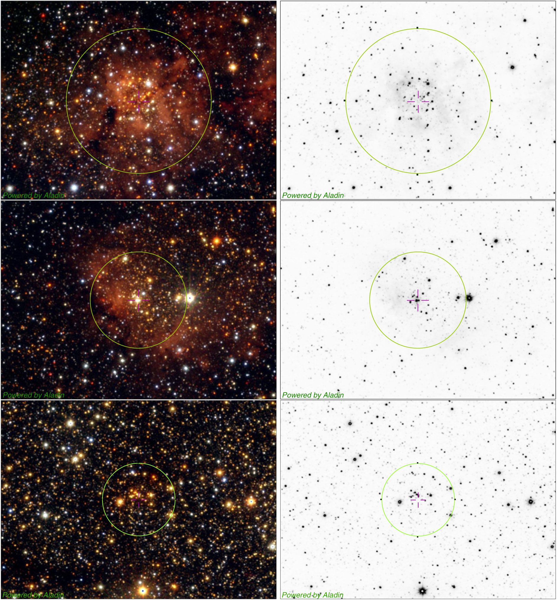
Figure 1. Three band ( $\text{JHK}_s$
) colour VVV image (left) and
$\text{JHK}_s$
) colour VVV image (left) and $K_S\text{-band}$
(right) for the three clusters projected on or near the W 31 complex. The images are centred at the clusters and have
$K_S\text{-band}$
(right) for the three clusters projected on or near the W 31 complex. The images are centred at the clusters and have $4.54' \times 3.28'$
each. The green circles (
$4.54' \times 3.28'$
each. The green circles ( $R=1.2'$
,
$R=1.2'$
, $R=0.8'$
, and
$R=0.8'$
, and $R=0.6'$
, respectively, from top to bottom) indicate the estimated cluster area. North is up and east is left.
$R=0.6'$
, respectively, from top to bottom) indicate the estimated cluster area. North is up and east is left.
The main cluster component in the complex is W 31-CL. It is associated with the Hii region $\text{G}\,10.2-0.3$
and the UCHii region
$\text{G}\,10.2-0.3$
and the UCHii region $\text{G}\,10.15-0.34$
. Blum et al. (Reference Blum, Damineli and Conti2001) studied the stellar content and emphasised the presence of several O stars and young stellar objects (YSOs). Based on the four O stars with K-band spectra, the authors determined a mean extinction of
$\text{G}\,10.15-0.34$
. Blum et al. (Reference Blum, Damineli and Conti2001) studied the stellar content and emphasised the presence of several O stars and young stellar objects (YSOs). Based on the four O stars with K-band spectra, the authors determined a mean extinction of $A_V=15.5\pm1.7\,\text{mag}$
. By assuming them as main sequence (MS), they derived a distance of
$A_V=15.5\pm1.7\,\text{mag}$
. By assuming them as main sequence (MS), they derived a distance of $3.4\,\text{kpc}$
and an age from the zero age main sequence (ZAMS) to 1 Myr.
$3.4\,\text{kpc}$
and an age from the zero age main sequence (ZAMS) to 1 Myr.
BDS 113 (Bica et al. Reference Bica, Dutra, Soares and Barbuy2003) is the W 31 complex component associated with the Hii region $\text{G}\,10.3-0.1$
, the UCHii
$\text{G}\,10.3-0.1$
, the UCHii $\text{G}\,10.3-0.15$
, and the IRAS source
$\text{G}\,10.3-0.15$
, and the IRAS source $\text{IRAS}\,18060-2005$
. Dewangan et al. (Reference Dewangan, Ojha, Grave and Mallick2015) analysed individual stars and continuum radio emission in the region of the mid-infrared bubble CN 148. They determined a mean cluster extinction of
$\text{IRAS}\,18060-2005$
. Dewangan et al. (Reference Dewangan, Ojha, Grave and Mallick2015) analysed individual stars and continuum radio emission in the region of the mid-infrared bubble CN 148. They determined a mean cluster extinction of $A_V\sim14\,\text{mag}$
and adopted a distance of
$A_V\sim14\,\text{mag}$
and adopted a distance of $2.2\,\text{kpc}$
, based on their references. They support triggered star formation, as a consequence of the expansion of the Hii region.
$2.2\,\text{kpc}$
, based on their references. They support triggered star formation, as a consequence of the expansion of the Hii region.
The most intriguing object in the set is the stellar cluster associated with SGR 1806-20 (Fuchs et al. Reference Fuchs, Mirabel, Chaty, Claret, Cesarsky and Cesarsky1999). Besides the Hii region $\text{G}\,10.0-0.3$
, it is associated with an X-ray counterpart
$\text{G}\,10.0-0.3$
, it is associated with an X-ray counterpart $\text{AX}\,1805.7-2025$
(Murakami et al. Reference Murakami, Tanaka, Kulkarni, Ogasaka, Sonobe, Ogawara, Aoki and Yoshida1994). These authors also support the hypothesis that SGRs are related to neutron stars. Figer et al. (Reference Figer, Najarro, Geballe, Blum and Kudritzki2005) studied the stellar content of the cluster SGR 1806-20 and concluded that it has three WR stars and one OB supergiant. The presence of one LBV star is supported by Eikenberry et al. (Reference Eikenberry2004), and Figer, Najarro, & Kudritzki (Reference Figer, Najarro and Kudritzki2004) argue that it is a binary system. The stellar cluster is deeply absorbed by dust, internally and/or in the foreground, as revealed by its mean extinction of
$\text{AX}\,1805.7-2025$
(Murakami et al. Reference Murakami, Tanaka, Kulkarni, Ogasaka, Sonobe, Ogawara, Aoki and Yoshida1994). These authors also support the hypothesis that SGRs are related to neutron stars. Figer et al. (Reference Figer, Najarro, Geballe, Blum and Kudritzki2005) studied the stellar content of the cluster SGR 1806-20 and concluded that it has three WR stars and one OB supergiant. The presence of one LBV star is supported by Eikenberry et al. (Reference Eikenberry2004), and Figer, Najarro, & Kudritzki (Reference Figer, Najarro and Kudritzki2004) argue that it is a binary system. The stellar cluster is deeply absorbed by dust, internally and/or in the foreground, as revealed by its mean extinction of $A_V\sim30\,\text{mag}$
(Corbel & Eikenberry Reference Corbel and Eikenberry2004).
$A_V\sim30\,\text{mag}$
(Corbel & Eikenberry Reference Corbel and Eikenberry2004).
The SGR 1806-20 distance determination is an open point in the literature (Bibby et al. Reference Bibby, Crowther, Furness and Clark2008; Corbel et al. Reference Corbel, Wallyn, Dame, Durouchoux, Mahoney, Vilhu and Grindlay1997; Corbel & Eikenberry Reference Corbel and Eikenberry2004). Some authors try to associate the SGR 1806-20 with the W 31 complex, but the results are not conclusive. Bibby et al. (Reference Bibby, Crowther, Furness and Clark2008) determined a distance of $8.7_{-1.5}^{+1.8}\,\text{kpc}$
, while Corbel & Eikenberry (Reference Corbel and Eikenberry2004) obtained
$8.7_{-1.5}^{+1.8}\,\text{kpc}$
, while Corbel & Eikenberry (Reference Corbel and Eikenberry2004) obtained $15.1_{-1.3}^{+1.5}\,\text{kpc}$
for the SGR and G 10.3-0.1, but
$15.1_{-1.3}^{+1.5}\,\text{kpc}$
for the SGR and G 10.3-0.1, but $4.5\pm0.6\,\text{kpc}$
for G 10.2-0.3 and G 10.6-0.4. Solving this puzzle is a goal of the present study.
$4.5\pm0.6\,\text{kpc}$
for G 10.2-0.3 and G 10.6-0.4. Solving this puzzle is a goal of the present study.
3. VVV photometry and methods
VVV is an European Southern Observatory (ESO) public survey that uses the VISTA telescope. It was designed to observe the bulge and part of the Milky Way disc in the NIR bands Z ( $0.87~{\mu} \text{m}$
), Y (
$0.87~{\mu} \text{m}$
), Y ( $1.02~\mu \text{m}$
), J (
$1.02~\mu \text{m}$
), J ( $1.25~\mu \text{m}$
), H (
$1.25~\mu \text{m}$
), H ( $1.64~\mu\text{m}$
), and
$1.64~\mu\text{m}$
), and $K_S$
(
$K_S$
( $2.14~\mu\text{m}$
). Among its goals is the study of RR-Lyrae stars in view of unveiling the central structure of the Galaxy (Minniti et al. Reference Minniti2010; Saito et al. Reference Saito2012).
$2.14~\mu\text{m}$
). Among its goals is the study of RR-Lyrae stars in view of unveiling the central structure of the Galaxy (Minniti et al. Reference Minniti2010; Saito et al. Reference Saito2012).
The 4.1-m VISTA telescope is located on Cerro Paranal, Chile. It has a Cassegrain focus and one instrument, the VIRCAM (Visual and InfraRed CAMera), described in details by Dalton et al. (Reference Dalton2006).
The basic data reduction steps are performed by the Cambridge Astronomical Survey Unit (CASU) through the VISTA Data Flow System (VDFS), which provides positions, magnitudes, and probable morphological type of the source. For details on the VVV photometry, we refer to Saito et al. (Reference Saito2012). In the present study, we used the aperture magnitudes provided by CASU.Footnote a
We employed the 2MASS photometry in the area to take into account saturation effects in the VVV photometry. The 2MASS photometry was obtained through the VizieRFootnote b tool, in which we extract circular regions centred on the cluster coordinates. The 2MASS magnitudes were converted into the VISTA Vegamag system according to the equations presented in Soto et al. (Reference Soto2013). Stars brighter than J, H, and $K_S$
$K_S$ $\sim11$
mag in the VISTA Vegamag were replaced by the respective 2MASS counterpart, considering a maximum spatial separation of
$\sim11$
mag in the VISTA Vegamag were replaced by the respective 2MASS counterpart, considering a maximum spatial separation of $0.5''$
(Lima et al. Reference Lima, Bica, Bonatto and Saito2014).
$0.5''$
(Lima et al. Reference Lima, Bica, Bonatto and Saito2014).
4. Star cluster analysis
The VVV Survey deals with heavily contaminated fields, and so clusters in those regions require the stellar background decontamination. Our group has performed the same kind of analysis for the NGC 6357 region (Lima et al. Reference Lima, Bica, Bonatto and Saito2014, and references therein), using CMDs, RDPs, and FS decontamination to probe the features of ECs. Next, we present a description of the methods used to analyse the VVV and 2MASS data of the selected stellar clusters.
4.1. FS decontamination
FS decontamination is an essential tool to study stellar clusters projected on dense fields, like towards the disc and bulge. Bonatto & Bica (2007a) developed an FS decontamination algorithm based on the total number of FS in the cluster region. This method was developed for 2MASS J, H, and K magnitudes, but we use an adapted version for the VVV photometry. Although the photometric and astrometric calibrations on the VVV data are performed via unsaturated 2MASS stars observed in each point, the VVV magnitudes are in the natural VISTA Vegamag system. The cluster area is defined based on RDPs (see Section 4.3) and the comparison field is chosen according to the projected distribution of stars and the presence of dust around the cluster. For each cluster analysed in the present work, we chose the ring, concentric to the cluster, that maximises the FS decontamination efficiency and yet preserves the evolutionary tracks seen in the CMDs (Figures 2 and 3).
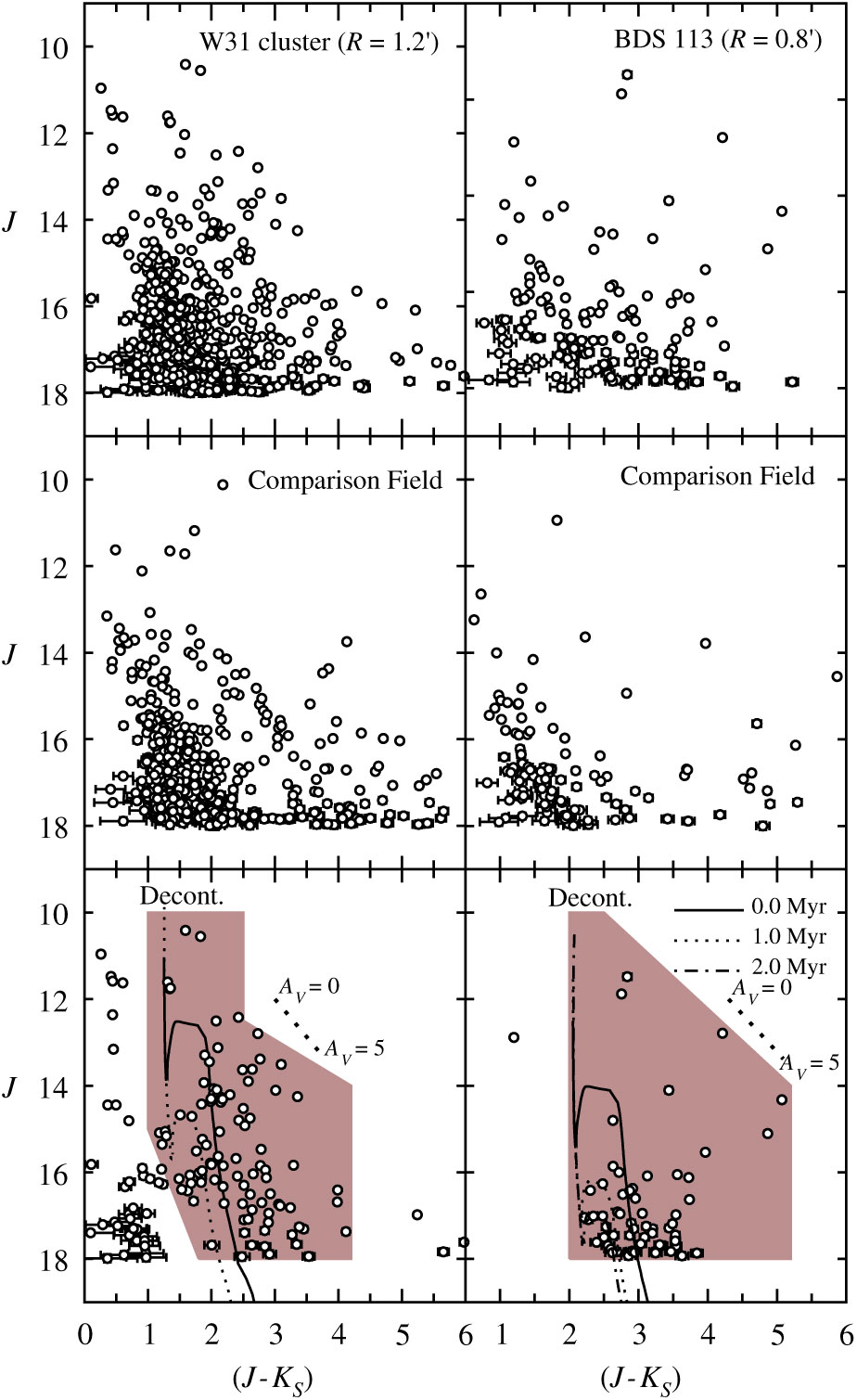
Figure 2. Left panels: CMDs of W 31-CL; right panels: CMDs of BDS 113. The top panels show the stars in the observed cluster area. Middle panels show the comparison field with the same projected area as the cluster, and the bottom ones the FS-decontaminated CMD. We overplot PARSEC isochrones.
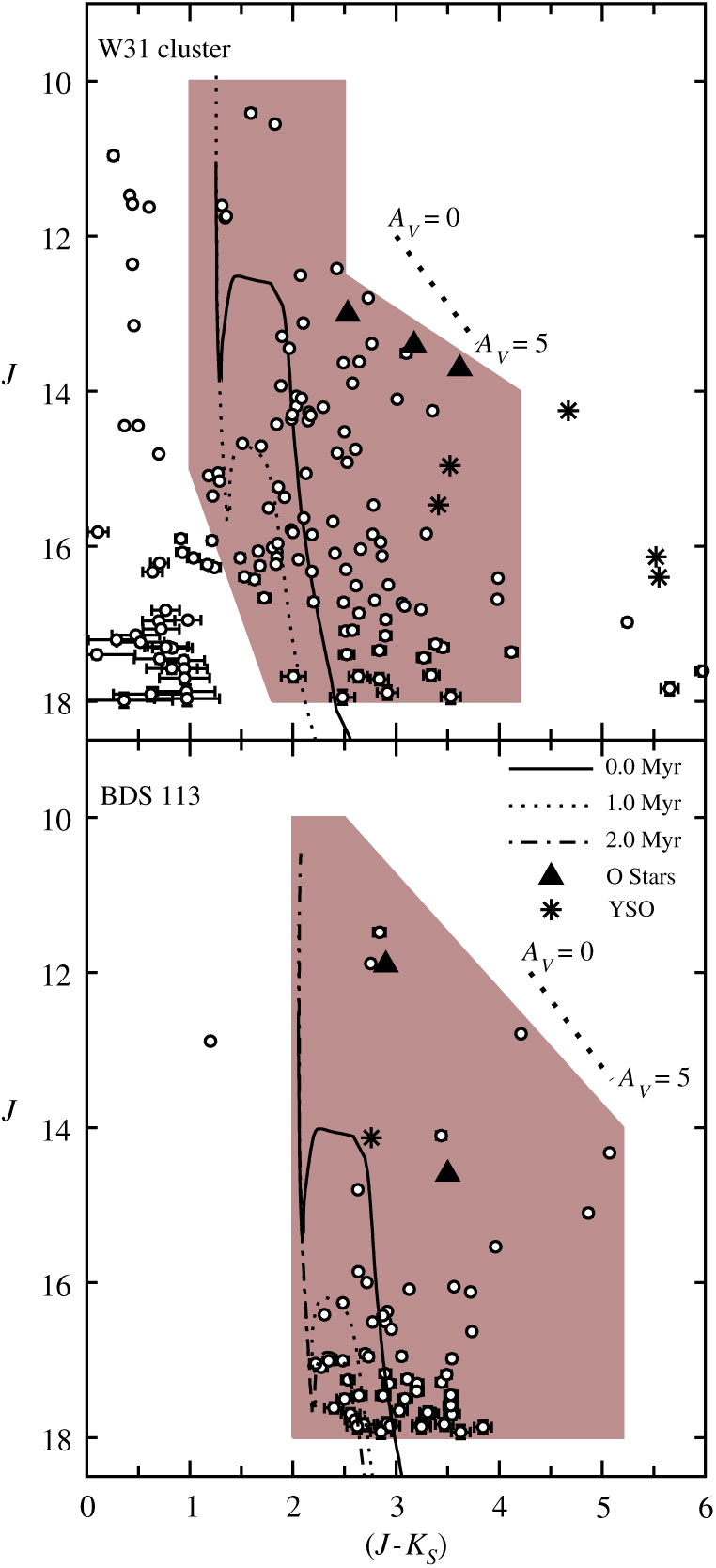
Figure 3. W 31-CL and BDS 113 CMDs: Same as bottom panels of Figure 2 with triangles and asterisms indicating the O stars and YSOs, respectively.
The method consists in dividing the stellar cluster CMD in a 3D grid with the magnitude J and the colours $( J-H)$
and
$( J-H)$
and $( J-K_S)$
as the axes, with a uncertainty of
$( J-K_S)$
as the axes, with a uncertainty of $\sim 1\sigma$
in each direction. Each grid unit is called a cell and has typical dimensions of
$\sim 1\sigma$
in each direction. Each grid unit is called a cell and has typical dimensions of $\Delta J=2.0\,\text{mag}$
and
$\Delta J=2.0\,\text{mag}$
and $\Delta( J-H)=\Delta( J-K_S)=0.5\,\text{mag}$
. These values are large enough to account for the photometric uncertainties and small enough to preserve the morphological properties of the evolutionary sequences. Subsequently, the expected number density of FS in each cell is calculated based on the number of FS in the comparison field with colours and magnitudes compatible with the ones of the cluster cells. The expected number of FS is randomly subtracted from each cell.
$\Delta( J-H)=\Delta( J-K_S)=0.5\,\text{mag}$
. These values are large enough to account for the photometric uncertainties and small enough to preserve the morphological properties of the evolutionary sequences. Subsequently, the expected number density of FS in each cell is calculated based on the number of FS in the comparison field with colours and magnitudes compatible with the ones of the cluster cells. The expected number of FS is randomly subtracted from each cell.
Another FS decontamination procedure is the CM filter. This method excludes the stars that are in different evolutionary sequences than the cluster and are outside to the filtered region in the CMD. We selected an area in the CMD in which the stars are more likely to be cluster members (brown areas in Figures 2–5). A limitation of the CM filter is that it does not eliminate FS with similar colours and magnitudes as the cluster ones, although it is a very useful tool in the investigation of structural parameters with RDPs (Figures 6 and 7) and the determination of mass functions.
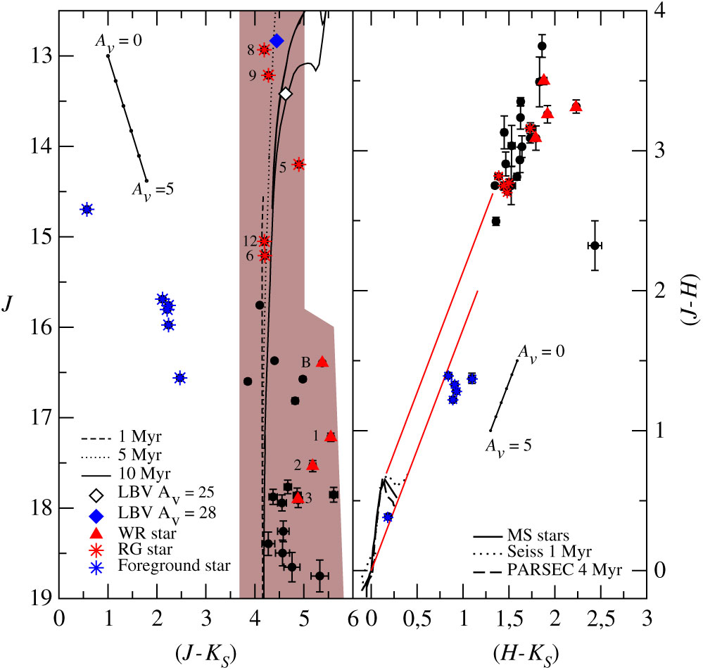
Figure 4. CMD (left panel) and CCD (right panel) of the SGR 1806-20 stars in common between the present photometry and the spectroscopic sample of Figer et al. (Reference Figer, Najarro, Geballe, Blum and Kudritzki2005). Classes and labels of probable members and foreground stars are indicated by different symbols and labels in the left panel. Isochrone model is zero age from PARSEC. The stars are within $R=0.6$
(Figure 1).
$R=0.6$
(Figure 1).
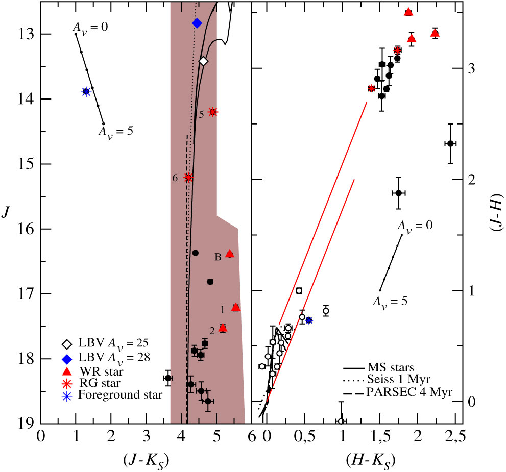

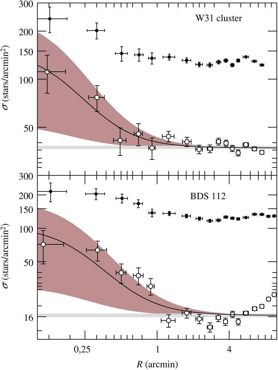
Figure 6. Observed (filled circles) and CM filtered (open circles) for W 31-CL and BDS 113 RDPs. A King-like profile was fitted (solid line). The $1\sigma$
background level is the light-shaded region.
$1\sigma$
background level is the light-shaded region.
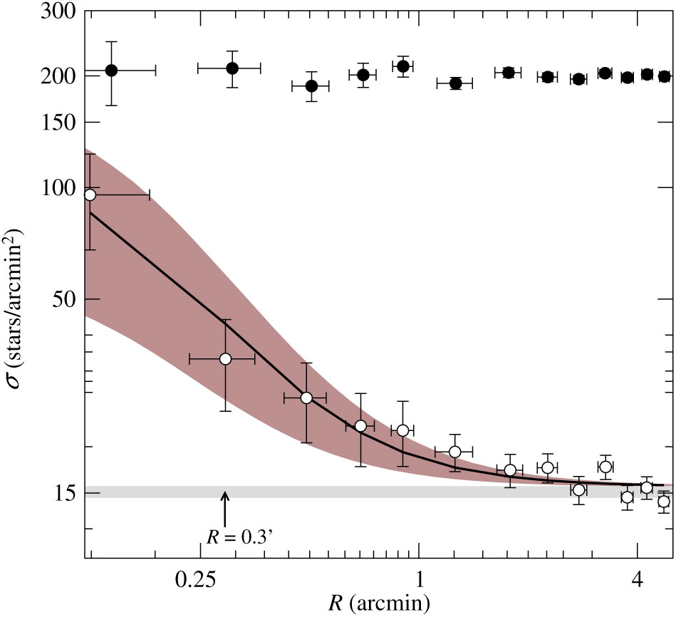
Figure 7. Observed and CM filtered RDPs for SGR 1806-20 in the top and bottom panels, respectively. Light-shaded region as in Figure 6.
In summary, we (i) build the FS-decontaminated CMDs in order to determine physical parameters of the stellar clusters, and then (ii) apply the CM filter to the ‘raw’ data to create the filtered RDPs. These two procedures are essential to remove the effects of the dense stellar fields and allow the determination of the stellar and structural parameters of interest.
4.2 Colour–magnitude diagrams
The FS-decontaminated CMDs are excellent tools to study stellar clusters. Through the isochrone fitting, we can determine the age, distance, and reddening of the cluster, which gives us a good idea of its physical scenario. The CMDs presented in Figure 2 show the following panels: (i) in the top panel, ‘raw’ CMDs comprise all the stars in the cluster area; (ii) the middle panel shows the comparison field CMDs with an area equal to cluster and the same range of colour and magnitude; (iii) in the bottom panel, FS-decontaminated CMDs show the isochrone fitting, the CM filters, and the reddening vector. All the CMDs, including Figures 3–5, are plotted in the VVV bands $J\times ( J-K_S)$
.
$J\times ( J-K_S)$
.
The models used to derive the distance, age, and reddening were the PARSECFootnote c from Bressan et al. (Reference Bressan, Marigo, Girardi, Salasnich, Dal Cero, Rubele and Nanni2012). They provide theoretical modelling for both MS and PMS stars (Bonatto & Bica Reference Bonatto and Bica2007a; Lima et al. Reference Lima, Bica, Bonatto and Saito2014).
The stellar parameters derived from the fitting are shown in Table 2, and include the value for the Galactocentric distance, $R_{GC}$
, calculated by adopting the Sun’s distance to the Galactic centre as
$R_{GC}$
, calculated by adopting the Sun’s distance to the Galactic centre as ${\rm R}_{\odot}=8.18\,\text{kpc}$
(Abuter et al. Reference Abuter2019) and the Cardelli, Clayton, & Mathis (Reference Cardelli, Clayton and Mathis1989) extinction relations with
${\rm R}_{\odot}=8.18\,\text{kpc}$
(Abuter et al. Reference Abuter2019) and the Cardelli, Clayton, & Mathis (Reference Cardelli, Clayton and Mathis1989) extinction relations with $R_V=3.1$
.
$R_V=3.1$
.
Table 2. Fundamental parameters for the stellar clusters in this study. $R_{GC}$
was calculated using
$R_{GC}$
was calculated using ${\rm R}_{\odot}=8.18\,\text{kpc}$
.
${\rm R}_{\odot}=8.18\,\text{kpc}$
.
4.2.1. W 31-CL
W 31-CL is the main infrared component of the star-forming complex W 31. Its decontaminated CMD (Figure 2, left bottom panel), for a selected radius of $1.2'$
and a comparison field of
$1.2'$
and a comparison field of $R=4'\text{--}6'$
, shows two MS stars and a spread PMS indicating a wide range of masses for the YSOs in this region. This feature is common in ECs. For the isochrone fitting, we select a range of isochrones that basically reproduces the evolutionary sequences in the CMD, and determine the best fit. Errors correspond to parameter shifts with which the neighbouring isochrones marginally fit the data.
$R=4'\text{--}6'$
, shows two MS stars and a spread PMS indicating a wide range of masses for the YSOs in this region. This feature is common in ECs. For the isochrone fitting, we select a range of isochrones that basically reproduces the evolutionary sequences in the CMD, and determine the best fit. Errors correspond to parameter shifts with which the neighbouring isochrones marginally fit the data.
Blum et al. (Reference Blum, Damineli and Conti2001) analysed spectroscopically O-type and YSOs in W 31. These stars basically lie along the reddening vector in the CMD of Figure 3 (top panel). We must be dealing with early type stars with a wide range of absorption values, probably owing to embedding dust caps or cocoons. Interestingly, the possible reddening slope of these embedded massive stars suggests a shift from the normal reddening law, as represented by the reddening vector in the top panel of Figure 3.
W 31-CL shows a considerable range of distances according to the literature, varying from 2.2 to $4.5\,\text{kpc}$
. However, the studies agree in the sense of a very young age, leading us to adopt two isochrones of zero age and 1 Myr. The parameters which led to the best estimate were
$4.5\,\text{kpc}$
. However, the studies agree in the sense of a very young age, leading us to adopt two isochrones of zero age and 1 Myr. The parameters which led to the best estimate were $E( J-K_S)=1.5\pm0.10$
,
$E( J-K_S)=1.5\pm0.10$
, $E(B-V)=2.59\pm0.95$
and
$E(B-V)=2.59\pm0.95$
and $A_V=8.72\pm0.58$
. The observed distance modulus is
$A_V=8.72\pm0.58$
. The observed distance modulus is ${(m-M)_J=15.80\pm0.50}$
, and the absolute is
${(m-M)_J=15.80\pm0.50}$
, and the absolute is ${(m-M)_0=13.27\pm0.53}$
. We determined a distance of
${(m-M)_0=13.27\pm0.53}$
. We determined a distance of $d_\odot=4.5\pm1.09\,\text{kpc}$
.
$d_\odot=4.5\pm1.09\,\text{kpc}$
.
4.2.2. BDS 113
The BDS 113-decontaminated CMD is shown in the right bottom panel of Figure 2. The cluster radius considered for the FS decontamination was $R=0.8'$
and a comparison field defined between
$R=0.8'$
and a comparison field defined between $R=6'\text{--}8'$
. It has no stars in the MS, so we based our fit only on the distribution of the PMS. There are two probable MS stars that show a
$R=6'\text{--}8'$
. It has no stars in the MS, so we based our fit only on the distribution of the PMS. There are two probable MS stars that show a $K_S$
excess, so they appear shifted to the right in the CMD. This CMD covers the same magnitude and colour range as the W 31-CL one, which may indicate that both are physically connected. The PMS distribution in the CMD is characterised by a spread in colour. Dewangan et al. (Reference Dewangan, Ojha, Grave and Mallick2015) identified the YSOs in this region based on their infrared excess emission, observed due to the presence of natal envelopes or circumstellar discs.
$K_S$
excess, so they appear shifted to the right in the CMD. This CMD covers the same magnitude and colour range as the W 31-CL one, which may indicate that both are physically connected. The PMS distribution in the CMD is characterised by a spread in colour. Dewangan et al. (Reference Dewangan, Ojha, Grave and Mallick2015) identified the YSOs in this region based on their infrared excess emission, observed due to the presence of natal envelopes or circumstellar discs.
Bik et al. (Reference Bik, Kaper, Hanson and Smits2005) identified two bright stars in the BDS 113 region, one is O8V-B2.5V and the other O5V-O6V. The CMD in the bottom panel of Figure 3 presents these two stars with the YSO 2MASS J18085079-2005195. As seen in W 31-CL, the O stars lie along the reddening vector. As expected, the YSO belongs to the PMS.
The fit of three PARSEC isochrones (0, 1, and 2 Myr) was necessary to better describe the PMS distribution. The best estimate provided the following parameters: $E( J-K_S)=2.30\pm0.10$
,
$E( J-K_S)=2.30\pm0.10$
, $E(B-V)= 3.97\pm0.95$
and
$E(B-V)= 3.97\pm0.95$
and $A_V=13.37\pm0.58$
; the observed and absolute distance modules are
$A_V=13.37\pm0.58$
; the observed and absolute distance modules are ${(m-M)_J=17.3\pm0.50}$
and
${(m-M)_J=17.3\pm0.50}$
and ${(m\,{-}\,M)_0=13.42\pm0.53}$
, respectively. With these values, we calculated a cluster distance of
${(m\,{-}\,M)_0=13.42\pm0.53}$
, respectively. With these values, we calculated a cluster distance of ${d_{\odot}=4.8\pm1.17\,\text{kpc}}$
, which is comparable with the determination for W 31-CL.
${d_{\odot}=4.8\pm1.17\,\text{kpc}}$
, which is comparable with the determination for W 31-CL.
4.2.3. SGR 1806-20
The literature has already placed the cluster in the direction of SGR 1806-20 at about $d_{\odot}=15\,\text{kpc}$
, but shorter distances were also considered (Section 2). The present study with VVV photometric accuracy is a remarkable opportunity to shed light on this issue. The FS-decontaminated CMD is shown in Figure 5. For the FS decontamination, we employ
$d_{\odot}=15\,\text{kpc}$
, but shorter distances were also considered (Section 2). The present study with VVV photometric accuracy is a remarkable opportunity to shed light on this issue. The FS-decontaminated CMD is shown in Figure 5. For the FS decontamination, we employ $R=0.3'$
, corresponding to the cluster high stellar density area (Section 5). The main difference from the previous two clusters is the high reddening, leading to a cluster sequence at
$R=0.3'$
, corresponding to the cluster high stellar density area (Section 5). The main difference from the previous two clusters is the high reddening, leading to a cluster sequence at ${( J-K_S)\sim5\,\text{mag}}$
. The position of the LBV is indicated, when applicable. Its relationship, or not, with the cluster must be studied. In Section 5, we also discuss the VVV counterpart of the cluster and field spectroscopic stars by Figer et al. (Reference Figer, Najarro, Geballe, Blum and Kudritzki2005).
${( J-K_S)\sim5\,\text{mag}}$
. The position of the LBV is indicated, when applicable. Its relationship, or not, with the cluster must be studied. In Section 5, we also discuss the VVV counterpart of the cluster and field spectroscopic stars by Figer et al. (Reference Figer, Najarro, Geballe, Blum and Kudritzki2005).
4.3 Radial density profiles
The projected RDPs can be used to study the radial structure of a stellar cluster (e.g. Bonatto & Bica Reference Bonatto and Bica2007a). They are built by computing the density of stars in concentric rings. The centre is determined by visual inspection of a cluster image. We use the data before the FS decontamination and the CM filtered data, respectively. Usually the latter enables to separate the cluster from the field better than the former, as already demonstrated by Bonatto & Bica (Reference Bonatto and Bica2007b).
The structural parameters are derived from the fit of a King-like profile (King Reference King1962) adapted to star counts, described by Equation (1), where $\sigma(R)$
,
$\sigma(R)$
, $\sigma_{\rm bg}$
, and
$\sigma_{\rm bg}$
, and $\sigma_{0}$
are the stellar, background, and peak densities, respectively; R and
$\sigma_{0}$
are the stellar, background, and peak densities, respectively; R and $R_c$
are the cluster and core radii, respectively. We use a two-parameter profile, which means that the
$R_c$
are the cluster and core radii, respectively. We use a two-parameter profile, which means that the $\sigma_{\rm bg}$
is fixed and determined directly from the RDP. These profiles also give an idea of the dynamical evolution of the cluster:
$\sigma_{\rm bg}$
is fixed and determined directly from the RDP. These profiles also give an idea of the dynamical evolution of the cluster:
 \begin{equation}
{\sigma(R)=\sigma_{\rm bg}+\sigma_{0}/\left[1+(R/R_c)^2\right].}
\label{eqn1}
\end{equation}
\begin{equation}
{\sigma(R)=\sigma_{\rm bg}+\sigma_{0}/\left[1+(R/R_c)^2\right].}
\label{eqn1}
\end{equation}
In Figure 6, we show the RDPs for the ECs W 31-CL and BDS 113. The filled circles are the observed and the open CM filtered RDPs. The two-parameter King-like profiles were fitted in the latter. Despite the small ages involved ( $\sim\!1\,\text{Myr}$
), the two clusters fit well the King-like profile, which led to the following fitting parameters:
$\sim\!1\,\text{Myr}$
), the two clusters fit well the King-like profile, which led to the following fitting parameters: $\sigma_{bg}=37.43\pm0.70\,\text{stars/arcmin}^2$
,
$\sigma_{bg}=37.43\pm0.70\,\text{stars/arcmin}^2$
, $\sigma_0=114.99\,\text{stars/arcmin}^2$
, and
$\sigma_0=114.99\,\text{stars/arcmin}^2$
, and $R_c=0.17\pm0.11'$
for W 31-CL;
$R_c=0.17\pm0.11'$
for W 31-CL; $\sigma_{bg}=16.44\pm0.50\,\text{stars/arcmin}^2$
,
$\sigma_{bg}=16.44\pm0.50\,\text{stars/arcmin}^2$
, $\sigma_0=87.67\pm0.14\,\text{stars/arcmin}^2$
, and
$\sigma_0=87.67\pm0.14\,\text{stars/arcmin}^2$
, and $R_c=0.23\pm0.14'$
for BDS 113. We also built the RDP for SGR 1806-20, presented in Figure 7. The use of the CM filter clearly enhanced the cluster structure, and likewise with the other two clusters, we fitted a King profile. The background field density is
$R_c=0.23\pm0.14'$
for BDS 113. We also built the RDP for SGR 1806-20, presented in Figure 7. The use of the CM filter clearly enhanced the cluster structure, and likewise with the other two clusters, we fitted a King profile. The background field density is $\sigma_{bg}=15.6\pm1.0\,\text{stars/arcmin}^2$
, and the peak density and core radius are
$\sigma_{bg}=15.6\pm1.0\,\text{stars/arcmin}^2$
, and the peak density and core radius are $\sigma_0=106.31\,\text{stars/arcmin}^2$
and
$\sigma_0=106.31\,\text{stars/arcmin}^2$
and $R_c=0.17\pm0.07'$
, respectively. The present clusters are young, so we do not expect relaxed systems. But interestingly, the three clusters can be fitted by a King-like profile. This is possibly related to formation and evolution of the clusters mimicking dynamically evolved profiles.
$R_c=0.17\pm0.07'$
, respectively. The present clusters are young, so we do not expect relaxed systems. But interestingly, the three clusters can be fitted by a King-like profile. This is possibly related to formation and evolution of the clusters mimicking dynamically evolved profiles.
For the SGR 1806-20, the cluster radius ( $R<0.6'$
) is first guessed from the cluster image and then optimised by the efficiency of the FS decontamination (Section 5.1). This value is the one that determines the CMD extractions (Figure 4).The central overdensity (
$R<0.6'$
) is first guessed from the cluster image and then optimised by the efficiency of the FS decontamination (Section 5.1). This value is the one that determines the CMD extractions (Figure 4).The central overdensity ( $R=0.3'$
) is indicated in the RDP and determines the CMD extraction in Figure 5. In this case, the input and output radii resulted the same. The same procedure was adopted for the other two clusters.
$R=0.3'$
) is indicated in the RDP and determines the CMD extraction in Figure 5. In this case, the input and output radii resulted the same. The same procedure was adopted for the other two clusters.
5. Discussion
VVV allowed us to obtain for the three clusters deeper CMDs than available in the literature. Decontamination was fundamental to interpret them and derive astrophysical parameters. The present study of the ECs W 31-CL and BDS 113 showed that they undoubtedly belong to the W 31 complex, and contain the ionising sources of the cloud. The connection with the corresponding Hii regions was suggested by Kim & Koo (Reference Kim and Koo2002) and Beuther et al. (Reference Beuther2011) in the radio domain. The distance determination for W 31-CL, $d_{\odot}= 4.5\,\text{kpc}$
, agrees with Blum et al. (Reference Blum, Damineli and Conti2001), however on a more straightforwardly basis by the present detection of the cluster PMS stars due to decontamination. We derive a distance of
$d_{\odot}= 4.5\,\text{kpc}$
, agrees with Blum et al. (Reference Blum, Damineli and Conti2001), however on a more straightforwardly basis by the present detection of the cluster PMS stars due to decontamination. We derive a distance of $d_{\odot}=4.8\,\text{kpc}$
for BDS 113, which is compatible with the W 31 complex distance. In fact, the PMS stars are the main constraint for the isochrone fitting. We emphasise that the present results were derived from stellar photometry, which is not dependent on the kinematic distance degeneracy problem (e.g. Russeil Reference Russeil2003).
$d_{\odot}=4.8\,\text{kpc}$
for BDS 113, which is compatible with the W 31 complex distance. In fact, the PMS stars are the main constraint for the isochrone fitting. We emphasise that the present results were derived from stellar photometry, which is not dependent on the kinematic distance degeneracy problem (e.g. Russeil Reference Russeil2003).
We analysed the structure of these clusters by fitting RDPs with King-like profiles. The RDPs of W 31-CL and BDS 113 could be basically described by this profile (Figure 6). Such King-like solutions are certainly due to formation and early dynamical evolution effects that mimic much older evolved cluster RDPs. Crowding and dust absorption can also affect the counts in such profiles in ECs (Camargo, Bonatto, & Bica Reference Camargo, Bonatto and Bica2015). It is noteworthy the importance of the decontamination procedures, in particular the CM filters (Bonatto & Bica Reference Bonatto and Bica2007a). The observed profiles are essentially flat in such dense stellar fields, as well as for clusters projected towards the central disc and bulge.
5.1 The nature of the cluster SGR 1806-20
In this subsection, we discuss the properties of the star cluster SGR 1806-20 to which the candidate LBV star and the soft gamma-ray repeater SGR 1806-20 are projected within $R=0.6'$
. In particular, we analyse colour–colour diagrams (CCDs), which bring out the absorption univocally (right panels of Figures 4 and 5).
$R=0.6'$
. In particular, we analyse colour–colour diagrams (CCDs), which bring out the absorption univocally (right panels of Figures 4 and 5).
The cluster is deeply embedded with $A_V=25\,\text{mag}$
, and this effect can be appreciated in the extreme red colours in the CMDs (left panels of Figures 4 and 5). This value is not at odds with
$A_V=25\,\text{mag}$
, and this effect can be appreciated in the extreme red colours in the CMDs (left panels of Figures 4 and 5). This value is not at odds with $A_V=28\,\text{mag}$
for the LBV (Figer et al. Reference Figer, Najarro, Geballe, Blum and Kudritzki2005). Figure 4 shows the CMD and CCD cross-identifications of the stars in the Keck spectroscopic analysis of Figer et al. (Reference Figer, Najarro, Geballe, Blum and Kudritzki2005) and the present photometry. Part of these stars are listed in Table 3, comparing possible luminous members with Bibby et al. (Reference Bibby, Crowther, Furness and Clark2008). The CCD indicates probable members along the loci of clusters isochrone models. The symbols and labels allow to deduce the foreground stars that are bluer than the cluster sequences, and the red giants (RGs) in the foreground put forward with spectroscopy by Figer et al. (Reference Figer, Najarro, Geballe, Blum and Kudritzki2005). In particular, the plots indicate that the LBV is unique, and with no rivals around in the CMD of Figure 4, the bright neighbouring stars in the CMD are foreground RGs. As to the luminous stellar content of the cluster, OI supergiants and WR stars populate the base of the CMDs. WR stars are redder than the cluster sequences in the CCD, which might suggest farther away. However, dust caps can occur making them probable members. All WR stars basically match other luminous members in J, so there occurs no luminosity conflict in the cluster.
$A_V=28\,\text{mag}$
for the LBV (Figer et al. Reference Figer, Najarro, Geballe, Blum and Kudritzki2005). Figure 4 shows the CMD and CCD cross-identifications of the stars in the Keck spectroscopic analysis of Figer et al. (Reference Figer, Najarro, Geballe, Blum and Kudritzki2005) and the present photometry. Part of these stars are listed in Table 3, comparing possible luminous members with Bibby et al. (Reference Bibby, Crowther, Furness and Clark2008). The CCD indicates probable members along the loci of clusters isochrone models. The symbols and labels allow to deduce the foreground stars that are bluer than the cluster sequences, and the red giants (RGs) in the foreground put forward with spectroscopy by Figer et al. (Reference Figer, Najarro, Geballe, Blum and Kudritzki2005). In particular, the plots indicate that the LBV is unique, and with no rivals around in the CMD of Figure 4, the bright neighbouring stars in the CMD are foreground RGs. As to the luminous stellar content of the cluster, OI supergiants and WR stars populate the base of the CMDs. WR stars are redder than the cluster sequences in the CCD, which might suggest farther away. However, dust caps can occur making them probable members. All WR stars basically match other luminous members in J, so there occurs no luminosity conflict in the cluster.
Table 3. Spectral and photometric information for the brighter stars in SGR 1806-20. (1) and (2) Star designations and classification from Figer et al. (Reference Figer, Najarro, Geballe, Blum and Kudritzki2005) and Bibby et al. (Reference Bibby, Crowther, Furness and Clark2008); (3), (4), and (5) J, ${(J-K_S),}$
and
${(J-K_S),}$
and $K_S$
magnitudes and colours obtained from the present VVV photometry; (6)
$K_S$
magnitudes and colours obtained from the present VVV photometry; (6) $K_S$
magnitude from Bibby et al. (Reference Bibby, Crowther, Furness and Clark2008). *The LBV columns (2) and (6) are from Figer et al. (Reference Figer, Najarro, Geballe, Blum and Kudritzki2005) while columns (3)–(5) are from 2MASS database, replacing saturated VVV star.
$K_S$
magnitude from Bibby et al. (Reference Bibby, Crowther, Furness and Clark2008). *The LBV columns (2) and (6) are from Figer et al. (Reference Figer, Najarro, Geballe, Blum and Kudritzki2005) while columns (3)–(5) are from 2MASS database, replacing saturated VVV star.
Figure 8 shows two circles that correspond to the radii $R\,{=}\,0.6'$
delimitating the area of the cross-identification above with Figer et al. (Reference Figer, Najarro, Geballe, Blum and Kudritzki2005), and
$R\,{=}\,0.6'$
delimitating the area of the cross-identification above with Figer et al. (Reference Figer, Najarro, Geballe, Blum and Kudritzki2005), and $R=0.3'$
. The latter radius encompasses the denser central cluster area. The LBV star is indicated. The dense inner zone is ideal to apply our decontamination method. It has been employed to ECs in many previous studies (e.g. Camargo, Bonatto, & Bica Reference Camargo, Bonatto and Bica2012; Camargo et al. Reference Camargo, Bonatto and Bica2015 and references therein), as well as to the W 31-CL and BDS 113 in the present study. The field subtraction method (Bonatto & Bica Reference Bonatto and Bica2007a) ensures that we decontaminate the FSs from the bulge, disc, and possible contamination from the W 31 complex.
$R=0.3'$
. The latter radius encompasses the denser central cluster area. The LBV star is indicated. The dense inner zone is ideal to apply our decontamination method. It has been employed to ECs in many previous studies (e.g. Camargo, Bonatto, & Bica Reference Camargo, Bonatto and Bica2012; Camargo et al. Reference Camargo, Bonatto and Bica2015 and references therein), as well as to the W 31-CL and BDS 113 in the present study. The field subtraction method (Bonatto & Bica Reference Bonatto and Bica2007a) ensures that we decontaminate the FSs from the bulge, disc, and possible contamination from the W 31 complex.
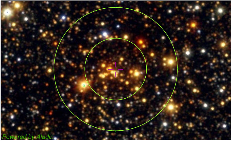
Figure 8. VVV image of SGR 1806-20, zoomed with respect to Figure 1. The outer circle has $R=0.6'$
corresponding to the cross-identification area of Figer et al.’s photometry and the present photometry. The inner circle has
$R=0.6'$
corresponding to the cross-identification area of Figer et al.’s photometry and the present photometry. The inner circle has $R=0.3'$
and is ideal for the decontamination method. North to the top, east to the left, and field dimensions of
$R=0.3'$
and is ideal for the decontamination method. North to the top, east to the left, and field dimensions of $2.23'\times1.35'$
.
$2.23'\times1.35'$
.
The SGR 1806-20 profile in Figure 7 shows that the cluster has a dense stellar core with $R=0.3'$
. It’s well populated, not a plain clump of bright stars, as at times reported in the early studies. Given its adequate structural properties, we applied decontamination (left panels of Figures 4 and 5). Other young dense clusters with rich backgrounds were analysed with VVV in a similar way, e.g. Pismis 24 and VVV CL 167 (Lima et al. Reference Lima, Bica, Bonatto and Saito2014). The decontaminated CMD and CCD (Figure 4) show that most foreground stars of Figer et al. (Reference Figer, Najarro, Geballe, Blum and Kudritzki2005) were removed, either by the down-sized area and the cleaning with respect to the field. A PARSEC isochrone describes both the LBV evolved state and clusters bright stars below. We estimate from shifting solutions for neighbouring isochrones at an age of
$R=0.3'$
. It’s well populated, not a plain clump of bright stars, as at times reported in the early studies. Given its adequate structural properties, we applied decontamination (left panels of Figures 4 and 5). Other young dense clusters with rich backgrounds were analysed with VVV in a similar way, e.g. Pismis 24 and VVV CL 167 (Lima et al. Reference Lima, Bica, Bonatto and Saito2014). The decontaminated CMD and CCD (Figure 4) show that most foreground stars of Figer et al. (Reference Figer, Najarro, Geballe, Blum and Kudritzki2005) were removed, either by the down-sized area and the cleaning with respect to the field. A PARSEC isochrone describes both the LBV evolved state and clusters bright stars below. We estimate from shifting solutions for neighbouring isochrones at an age of $10\pm4\,\text{Myr}$
and a heliocentric distance of
$10\pm4\,\text{Myr}$
and a heliocentric distance of $d_{\odot}=8.0\pm1.9\,\text{kpc}$
. The fitting parameters are as follows:
$d_{\odot}=8.0\pm1.9\,\text{kpc}$
. The fitting parameters are as follows: $E( J-K_S)=4.35\pm0.10$
,
$E( J-K_S)=4.35\pm0.10$
, $E(B-V)= 7.52\pm0.95$
, and
$E(B-V)= 7.52\pm0.95$
, and $A_V\,{=}\,25.29\pm0.58$
; the observed and absolute distance modules are
$A_V\,{=}\,25.29\pm0.58$
; the observed and absolute distance modules are ${(m-M)_J=21.86\pm0.50}$
and
${(m-M)_J=21.86\pm0.50}$
and ${(m-M)_0=14.53\pm0.53}$
, respectively. They represent the best fitting solutions for the CMDs in Figures 4 and 5.
${(m-M)_0=14.53\pm0.53}$
, respectively. They represent the best fitting solutions for the CMDs in Figures 4 and 5.
The discovery and analysis of the new star clusters with VVV, both young and old, in the bulge or in the central disc, have been recently boosted with the VVV Survey. Examples are the new globular cluster Minni 22 and a series of new candidates (Minniti et al. Reference Minniti2017). Crowding in the bulge and central disc fields can make them virtually inconspicuous in the VVV images, but they correspond to high stellar overdensities, in particular Minni 22 is $30\,\sigma$
above the background. In order to further stress the occurrence of a rather populous cluster in the direction of the soft-gamma ray source SGR 1806-20, we use the first version of the VVV Infrared Astrometric Catalogue (VIRAC, Smith et al. Reference Smith2018). The proper motion (PM) components
$30\,\sigma$
above the background. In order to further stress the occurrence of a rather populous cluster in the direction of the soft-gamma ray source SGR 1806-20, we use the first version of the VVV Infrared Astrometric Catalogue (VIRAC, Smith et al. Reference Smith2018). The proper motion (PM) components $\mu_{\alpha\cos\delta}$
and
$\mu_{\alpha\cos\delta}$
and $\mu_{\delta}$
in
$\mu_{\delta}$
in $\text{masyr}^{-1}$
for the FSs and the FS-decontaminated stars of the SGR 1806-20 are presented in Figure 9. The cluster stars show very similar PM values internally, specially the OB and WR stars, while the field has more spread values with an offset. This indicates that the stars in blue are physically connected. VVV VIRAC efforts so far deal with magnitude ranges where the LBV is saturated, and consequently not present in the PM catalogues currently available for the region (e.g. VIRAC and Gaia, Smith et al. Reference Smith2018; Gaia Collaboration et al. Reference Collaboration2018).
$\text{masyr}^{-1}$
for the FSs and the FS-decontaminated stars of the SGR 1806-20 are presented in Figure 9. The cluster stars show very similar PM values internally, specially the OB and WR stars, while the field has more spread values with an offset. This indicates that the stars in blue are physically connected. VVV VIRAC efforts so far deal with magnitude ranges where the LBV is saturated, and consequently not present in the PM catalogues currently available for the region (e.g. VIRAC and Gaia, Smith et al. Reference Smith2018; Gaia Collaboration et al. Reference Collaboration2018).
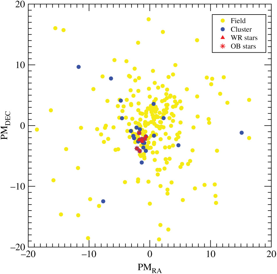
Figure 9. VVV PM for all the stars within the cluster radius ( $R=0.6'$
, yellow dots), and for the field-decontaminated stars (blue dots) in SGR 1806-20 (the same stars as in Figure 4). RA PM corresponds to
$R=0.6'$
, yellow dots), and for the field-decontaminated stars (blue dots) in SGR 1806-20 (the same stars as in Figure 4). RA PM corresponds to $\mu_{\alpha\cos\delta}$
. The WR and OB stars are indicated as red triangles and red asterisks.
$\mu_{\alpha\cos\delta}$
. The WR and OB stars are indicated as red triangles and red asterisks.
Finally, we emphasise that in the past, there has been considerable spread in distance estimates of this cluster. The most recent one was by Bibby et al. (Reference Bibby, Crowther, Furness and Clark2008) leading to a cluster distance range of $7.2\text{--}10.4\,\text{kpc}$
. The present value of
$7.2\text{--}10.4\,\text{kpc}$
. The present value of $8.0\pm1.95\,\text{kpc}$
is thus compatible, settling the distance issue. We conclude that the cluster SGR 1806-20 is unrelated to the W 31 complex, being almost a factor of
$8.0\pm1.95\,\text{kpc}$
is thus compatible, settling the distance issue. We conclude that the cluster SGR 1806-20 is unrelated to the W 31 complex, being almost a factor of $\approx1.8$
more distant.
$\approx1.8$
more distant.
6. Conclusions
We employed VVV photometry to study young clusters projected on or nearby the W 31 star-forming complex. We used CMDs and RDPs to derive cluster parameters, including structural ones. The W 31 cluster and BDS 113 belong to the complex at a distance of $d_{\odot}=4.5-4.8\,\text{kpc}$
. These two clusters appears to be the youngest generation in the complex with ages around
$d_{\odot}=4.5-4.8\,\text{kpc}$
. These two clusters appears to be the youngest generation in the complex with ages around $1\,\text{Myr}$
. Note that the CMDs of W 31-CL and BDS 113 show clear PMS content as in clusters like Pismis 24 in the nearby complex NGC6357 (Lima et al. Reference Lima, Bica, Bonatto and Saito2014).
$1\,\text{Myr}$
. Note that the CMDs of W 31-CL and BDS 113 show clear PMS content as in clusters like Pismis 24 in the nearby complex NGC6357 (Lima et al. Reference Lima, Bica, Bonatto and Saito2014).
In the case of the SGR 1806-20, we cross-identified the spectroscopic classification by Figer et al. (Reference Figer, Najarro, Geballe, Blum and Kudritzki2005) with the present VVV/2MASS photometry in view of constraining the cluster parameters. We show how the stellar content, in terms of the LBV, WR, and O supergiant stars are mostly cluster members, and other stars belong to the foreground. The present cluster distance of $8.0\,\text{kpc}$
is comparable with Bibby et al. (Reference Bibby, Crowther, Furness and Clark2008). We conclude that the cluster SGR 1806-20 is a factor of 1.7 more distant and significantly older than the W 31 complex, and thus not physically related to it.
$8.0\,\text{kpc}$
is comparable with Bibby et al. (Reference Bibby, Crowther, Furness and Clark2008). We conclude that the cluster SGR 1806-20 is a factor of 1.7 more distant and significantly older than the W 31 complex, and thus not physically related to it.
Acknowledgements
We thank the anonymous referee for the comments that helped to improve the text. This study was financed in part by the Coordenação de Aperfeiçoamento de Pessoal de Nível Superior - Brasil (CAPES) - Finance Code 001, Conselho Nacional de Desenvolvimento Científico e Tecnológico (CNPq), and Fundação de Amparo à pesquisa do Estado do RS (FAPERGS). This publication makes use of data products from the 2MASS, which is a joint project of the University of Massachusetts and the Infrared Processing and Analysis Center/California Institute of Technology, funded by the National Aeronautics and Space Administration and the National Science Foundation. R.K.S. acknowledges support from CNPq/Brazil through projects 308968/2016-6 and 421687/2016-9.


