


1. Introduction
Although pulsars were discovered in 1967 (Hewish et al. Reference Hewish, Bell, Pilkington, Scott and Collins1968), the exact mechanism by which they emit electromagnetic radiation is far from being understood. The pulsar emission mechanism is often described using models that include a plasma-filled magnetosphere that co-rotates with the pulsar (Goldreich & Julian Reference Goldreich and Julian1969). However, an emission mechanism that can successfully explain all pulsar emission characteristics, including spectral turnover and nulling, has not yet been advanced. Radio spectra of pulsars provide important clues, but accurate spectral data are lacking for the majority of pulsars.
Measurements of flux densities are important for inferring pulsar radio luminosities and energetics, as well as for detailed spectral analysis. However, producing accurate pulsar flux densities is challenging for several reasons. Firstly, pulsars scintillate due to the interstellar medium, which can cause the apparent flux density to fluctuate from a factor of 2 to an order of magnitude, particularly at low frequencies, depending on their galactic latitude and the choice of instrumental parameters (e.g. observing bandwidth and time duration), on timescales up to weeks and months (e.g. Swainston et al. Reference Swainston2021; Bhat et al. Reference Bhat2018; Bell et al. Reference Bell2016). Obtaining flux measurements, therefore, requires observing campaigns much longer than the scintillation timescale. Secondly, flux density measurements require extensive knowledge of the telescope to account for antenna temperature, beam shape, etc. Furthermore, in the case of pulsars with severely broadened pulse profiles (due to temporal broadening resulting from multipath scattering), reliable measurements may require imaging rather than time-domain techniques. Despite these difficulties, many accurate flux density measurements have been taken over the last several decades (e.g. Izvekova et al. Reference Izvekova, Kuzmin, Malofeev and Shitov1981; Taylor et al. Reference Taylor, Manchester and Lyne1993; Lorimer et al. Reference Lorimer, Yates, Lyne and Gould1995; Malofeev et al. Reference Malofeev, Malov and Shchegoleva2000; Hobbs et al. Reference Hobbs, Manchester, Teoh, Hobbs, Camilo and Gaensler2004a; Bilous et al. Reference Bilous2016; Han et al. Reference Han, Wang, Xu and Han2016; Johnston & Kerr Reference Johnston and Kerr2018; Jankowski et al. Reference Jankowski2019; Sanidas et al. Reference Sanidas2019). However, there is currently no catalogue designed to record pulsar flux density measurements at arbitrary frequencies. Researchers are obliged to do extensive literature reviews, find the publications that contain flux density measurements of pulsars they are interested in, and extract the information from them. This exercise is a time-consuming task that is prone to error.
There is no complete theoretical model for pulsar spectra. For this reason, we use several empirical models as no single model can accurately fit the variety of pulsars’ spectra. Deciding which models to use and which is best for each pulsar requires sophisticated statistical techniques. Jankowski et al. (Reference Jankowski, van Straten, Keane, Bailes, Barr, Johnston and Kerr2018) has detailed a method for deciding on the best model using the Akaike information criterion (AIC), which measures the information each model retains without overfitting. This is applied to various spectral models used throughout the literature (see Section 3.1). Their choice of method and implementation can result in different results compared to other researchers with the same data.
We have implemented the methodology of Jankowski et al. (Reference Jankowski, van Straten, Keane, Bailes, Barr, Johnston and Kerr2018) in pulsar_spectra ,Footnote a a fully featured spectral fitting python software package. It includes all five models listed above and can be easily extended to include others. pulsar_spectra also contains a catalogue of flux density measurements from several publications. pulsar_spectra is open-source; researchers can upload measurements from new publications into the catalogue, which are then available to all. The software has already been used in Lee et al. (Reference Lee, Bhat, Sokolowski, Swainston, Ung, Magro and Chiello2022).
The remainder of this paper is organised as follows. We will first explain the implementation of the catalogue and its benefits in Section 2. Then in Section 3, we discuss the method used to determine the best spectral fit. Finally, in Section 4, we demonstrate how to use the software.
2. Catalogue
There is currently no pulsar catalogue exclusively for flux density measurements. The ATNF pulsar catalogue (version v1.67; Manchester et al. Reference Manchester, Hobbs, Teoh and Hobbs2005) does maintain a large collection of published flux densities, but the frequency at which they are measured is not always accurate. Flux densities measured at frequencies other than a set of pre-selected frequencies (currently 26, ranging from 30 MHz to 150 GHz) are typically recorded at the nearest listed frequency, which can lead to inaccurate spectral fits if the frequency and flux density values in the catalogue are taken at face value. Moreover, the catalogue’s design prohibits multiple measurements at the same or similar frequencies, with only the most recent measurement recorded at any given (approximate) frequency.
Researchers are currently obliged to conduct their own extensive literature reviews to find the publications that contain flux density measurements of pulsars they are interested in and extract the relevant information from them. This is a time-consuming task and, because there is no central place to store this information, it is duplicated effort by each researcher.
To allow researchers to acquire accurate flux density measurements with minimal effort, we have created an open-source catalogue within pulsar_spectra . The catalogue consists of dictionaries in the form of a YAML file for each included publication. These YAML files contain all the flux density measurements and their uncertainty in mJy and their frequencies in MHz for each pulsar. If the original authors gave no flux density uncertainty, we assumed a conservative relative uncertainty of 50%, following earlier work (Sieber Reference Sieber1973; Jankowski et al. Reference Jankowski, van Straten, Keane, Bailes, Barr, Johnston and Kerr2018). This catalogue can easily be collected using a python function and combined with new results to produce a pulsar spectral fit (as demonstrated in Section 4).
When using the flux density values from the ATNF to fit a pulsar, most researchers know that the values are inaccurate due to the select frequencies of the ATNF (see the left plots in Figure 1). They would then extract the publications’ true flux density and frequency values to create a more accurate fit. With pulsar_spectra , this is rarely required as our catalogue can use any frequency value (see the right plots in Figure 1). This frequency flexibility also allows us to include papers, such as Murphy et al. (Reference Murphy2017) and Johnston, Karastergiou, & Willett (Reference Johnston, Karastergiou and Willett2006), which have flux density measurements at many frequencies. The four pulsars in Figure 1 are examples of a different and more accurate fit using pulsar_spectra without manually extracting values from the publications.

Figure 1. Left: A spectral fit using only the flux density values from the ATNF pulsar catalogue. Right: A spectral fit using only the flux density values from the pulsar_spectra catalogue. As demonstrated through these examples, the pulsar_spectra catalogue is able to accommodate many more flux density values than those available in the ATNF pulsar catalogue and hence can yield more accurate spectral fits.
2.1. Currently included and future publications
The catalogue is designed to be a community-maintained, open-source catalogue that prevents duplicated effort. We have currently added 34 publications to the database, which are shown in Table 1. This is not a complete list of pulsar flux density publications and is likely to favour Southern-sky (declination $\delta < 0$
) pulsars. As researchers use this catalogue, they can add new flux density measurements (or historical ones that are not already included), which can then be made available for other researchers.
$\delta < 0$
) pulsars. As researchers use this catalogue, they can add new flux density measurements (or historical ones that are not already included), which can then be made available for other researchers.
Table 1. The publications included in version 2.0 of pulsar_spectra . For an up to date table see the documentation.

To make it easier for other researchers to include new publications in the catalogue, we have created a script to convert a simple CSV into the required YAML format that the catalogue requires, as explained in our documentation.Footnote b They can use this to make a pull request, and this publication will be included in the next release of pulsar_spectra . We will keep an up-to-date table of publications Footnote c to make it easier to cite the data and to encourage authors to upload their own published results.
When comparing the current state of the catalogue to the ATNF catalogue (see Table 2), the pulsar_spectra catalogue already contains a larger sample of pulsar flux density measurements. We hope that the open-source nature of our catalogue and the ease of uploading new publications’ flux density measurements will allow our catalogue to grow rapidly in the coming years.
Table 2. This table compares the current progress of our catalogue compared to the ATNF. As users continue to add publications the catalogue will grow.

3. Pulsar spectral fitting
Flux density measurements obtained using different telescopes are subject to different systematic errors due to the telescope’s observing set-up and varying levels of reliability of the calibration procedures. These systematic errors make robust modelling of spectral fits complicated. Jankowski et al. (Reference Jankowski, van Straten, Keane, Bailes, Barr, Johnston and Kerr2018) developed a method of modelling and objectively classifying spectra which are composed of disparate data from the literature, and our approach is adapted from this work. We now summarise the Jankowski et al. (Reference Jankowski, van Straten, Keane, Bailes, Barr, Johnston and Kerr2018) method used in our software.
To reduce the effect of underestimated uncertainties on outlier points in a given fit, the least squares function is modified from the regular quadratic loss to a linear loss once the residuals exceed a pre-chosen threshold. In this way, outlier data are penalised, and as a result any measurements that are less reliable are less likely to skew the model fit. In pulsar_spectra , we implement this using the Huber loss function, defined as:
 \begin{equation} \rho = \begin{cases} \dfrac{1}{2}t^2 & \mathrm{if}\:|t|<k \\[12pt] k|t|-\dfrac{1}{2}k^2 & \mathrm{if}\:|t|\geq k \end{cases},\end{equation}
where t is a residual (i.e. the difference between the model and the measurement) and k is the threshold that defines which points are considered outliers (Huber Reference Huber1964). We use a value of $k = 1.345$
, for which Huber has shown to be 95% as efficient at parameter estimation as an ordinary least squares estimator operating on data from a Gaussian distribution. We hence define a robust cost function:
$k = 1.345$
, for which Huber has shown to be 95% as efficient at parameter estimation as an ordinary least squares estimator operating on data from a Gaussian distribution. We hence define a robust cost function:
 \begin{equation} \beta = \sum_i^N \begin{cases} \dfrac{1}{2}\left(\dfrac{f_i-y_i}{\sigma_{y,i}}\right)^2 & \mathrm{if}\:\left|\dfrac{f_i-y_i}{\sigma_{y,i}}\right|<k \\[15pt] k\left|\dfrac{f_i-y_i}{{\sigma}_{y,i}}\right|-\dfrac{1}{2}k^2 & \mathrm{otherwise} \end{cases},\end{equation}
where $f_i$
are the values of the model function at the frequencies of the measured flux densities
$f_i$
are the values of the model function at the frequencies of the measured flux densities $y_i$
, and
$y_i$
, and $\sigma_{y,i}$
are the corresponding uncertainties of the flux densities.
$\sigma_{y,i}$
are the corresponding uncertainties of the flux densities.
The cost function is minimised using migrad, a robust minimisation algorithm implemented in the minuit c++ library (as described in James & Roos Reference James and Roos1975) which is accessible through the python interface iminuit.Footnote d migrad uses a combination of Newton steps and gradient descents to converge to a local minimum. The Estimated Distance to Minimum (EDM) is used to define a convergence criterion in terms of a specified tolerance (which must be met for the minimisation to be considered successful), which is set to a value of $5 \times 10^{-6}$
. The uncertainties are computed at the 1
$5 \times 10^{-6}$
. The uncertainties are computed at the 1 $\sigma$
level from the diagonal elements of the parameter covariance matrix using the hesse error calculator.
$\sigma$
level from the diagonal elements of the parameter covariance matrix using the hesse error calculator.
3.1. Spectral models
We have currently implemented the five spectral models that have distinct spectral shapes from Jankowski et al. (Reference Jankowski, van Straten, Keane, Bailes, Barr, Johnston and Kerr2018). While these five models are sufficient for describing the spectra for the vast majority of pulsars, our software is flexible enough to allow the addition of more spectral models easily, as explained here.Footnote e
The choice of the reference frequency, $\nu_0$
, in the following models can affect the spectral fits as the data closer to the reference frequency are given more weight. To make the weighting of the fit as even as possible, we select
$\nu_0$
, in the following models can affect the spectral fits as the data closer to the reference frequency are given more weight. To make the weighting of the fit as even as possible, we select $\nu_0$
as the geometric average (average in log-space) of the minimum and maximum frequencies in the spectral fit (
$\nu_0$
as the geometric average (average in log-space) of the minimum and maximum frequencies in the spectral fit ( $\nu_{\textrm{min}}$
and
$\nu_{\textrm{min}}$
and $\nu_{\textrm{max}}$
, respectively):
$\nu_{\textrm{max}}$
, respectively):
 \begin{equation} \log_{10}\nu_0 = \frac{1}{2}\left(\log_{10}\nu_{\textrm{min}}+\log_{10}\nu_{\textrm{max}}\right).\end{equation}
This method has also been adopted in previous work (e.g. Bilous et al. Reference Bilous2016). We define the scaling constant in the following spectral models as c.
We shall now describe the spectral models and provide example pulsars that are best fit by each of these models as of pulsar_spectra version 2.0.
3.1.1. Simple power law
The simple power law is linear in log-space and the most common spectral model. Some examples of this include PSRs J0034-0534 (see Figure 2), J1328-4357, and J0955-5304. The model takes the form:
 \begin{equation} S_\nu = c \left( \frac{\nu}{\nu_0} \right)^\alpha,\end{equation}
where $\alpha$
is the spectral index. The fit parameters are
$\alpha$
is the spectral index. The fit parameters are $\alpha$
and c.
$\alpha$
and c.
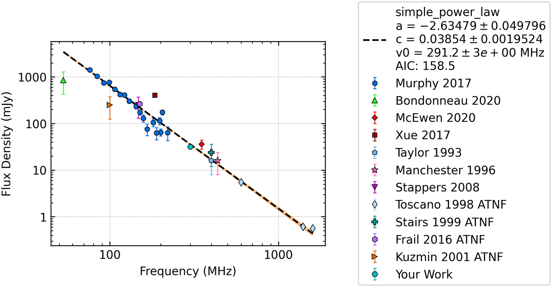
Figure 2. The spectral fit to the flux density measurements of PSR J0034-0534 created using the pulsar_spectra software and only the 11 lines of code shown in Listing 1.
3.1.2. Broken power law
The broken power law is the equivalent of two simple power laws that differ at a spectral break frequency. Variations on this model have been applied in other fields of astrophysics, such as the smoothly broken power law, which is characterised by an additional parameter describing the width of the transition (e.g. Ryde Reference Ryde1999). Pulsar spectra are traditionally fit with sharply broken power laws, characterised by only four free parameters (e.g. Sieber Reference Sieber1973; Murphy et al. Reference Murphy2017). Some examples of broken power law fits include PSRs J0437-4715 (see Figure 1), J0452-1759 and J0820-1350. The model takes the form:
 \begin{equation} S_\nu = c\begin{cases} \left( \dfrac{\nu}{\nu_0} \right)^{\alpha_1} & \mathrm{if}\: \nu \leq \nu_b \\[12pt] \left( \dfrac{\nu}{\nu_0} \right)^{\alpha_2} \left( \dfrac{\nu_b}{\nu_0} \right)^{\alpha_1-\alpha_2} & \mathrm{otherwise} \\ \end{cases},\end{equation}
where $\nu_b$
is the frequency of the spectral break,
$\nu_b$
is the frequency of the spectral break, $\alpha_1$
the spectral index before and
$\alpha_1$
the spectral index before and $\alpha_2$
the one after the break. The fit parameters are
$\alpha_2$
the one after the break. The fit parameters are $\alpha_1$
,
$\alpha_1$
, $\alpha_2$
,
$\alpha_2$
, $\nu_b$
, and c.
$\nu_b$
, and c.
3.1.3. Log-parabolic spectrum
This model has been used to describe the spectra of radio galaxies (e.g. Baars et al. Reference Baars, Genzel, Pauliny-Toth and Witzel1977) and curved pulsar spectra (Bates, Lorimer, & Verbiest Reference Bates, Lorimer and Verbiest2013; Dembska et al. Reference Dembska, Kijak, Jessner, Lewandowski, Bhattacharyya and Gupta2014). Some examples of log-parabolic spectra include PSRs J1141-6545 (see Figure 1), J1313+0931 and J0837+0610. The model takes the form:
 \begin{equation} \mathrm{log}_{10} S_\nu = a \left [ \mathrm{log}_{10} \left ( \frac{\nu}{\nu_0} \right ) \right]^2 + b \, \mathrm{log}_{10} \left ( \frac{\nu}{\nu_0} \right ) + c,\end{equation}
where a is the curvature parameter and b is the spectral index for $a = 0$
. The fit parameters are a, b, and c.
$a = 0$
. The fit parameters are a, b, and c.
3.1.4. Power law with high-frequency cut-off
This model, also known as the hard cut-off model, is based on the coherent emission model developed by Kontorovich & Flanchik (Reference Kontorovich and Flanchik2013). At high frequencies, its flux quickly trends towards zero before a cut-off frequency. An example of this is PSR J1751-4657 (see Figure 1). The model takes the form:
 \begin{equation} S_\nu = c\left( \frac{\nu}{\nu_0} \right)^{\alpha} \left ( 1 - \frac{\nu}{\nu_c} \right ),\qquad \nu < \nu_c,\end{equation}
where $\alpha$
is the spectral index and
$\alpha$
is the spectral index and $\nu_c$
is the cut-off frequency. The fit parameters are
$\nu_c$
is the cut-off frequency. The fit parameters are $\alpha$
,
$\alpha$
, $\nu_c$
and c.
$\nu_c$
and c.
3.1.5. Power law with low-frequency turnover
This model exhibits a power law at high frequencies with a turnover at low frequencies. The curve of this turnover can give us clues about the nature of the pulsar emission mechanism (Izvekova et al. Reference Izvekova, Kuzmin, Malofeev and Shitov1981; Kijak et al. Reference Kijak, Gupta and Krzeszowski2007). Some examples of this include PSRs J0953+0755 (see Figure 1), J1543+0929 and J0034-0721. The model takes the form:
 \begin{equation} S_\nu = c\left( \frac{\nu}{\nu_0} \right)^{\alpha} \exp\left [ \frac{\alpha}{\beta} \left( \frac{\nu}{\nu_{peak}} \right)^{-\beta} \right ],\end{equation}
where $\alpha$
is the spectral index,
$\alpha$
is the spectral index, $\nu_{peak}$
is the turnover frequency, and
$\nu_{peak}$
is the turnover frequency, and $0 < \beta \leq 2.1$
determines the smoothness of the turnover. The fit parameters are
$0 < \beta \leq 2.1$
determines the smoothness of the turnover. The fit parameters are $\alpha$
,
$\alpha$
, $\nu_{peak}$
,
$\nu_{peak}$
, $\beta$
and c.
$\beta$
and c.
3.2. Comparing models
To compare five models (described in Section 3.1), we require a comparison metric that accounts for a different number of fit parameters. We use the AIC, which is a measure of how much information the model retains about the data without overfitting. In other words, a model with more fit parameters is only rated better if the fit is sufficiently improved. It was implemented as:
 \begin{equation} \mathrm{AIC}=2\beta_\mathrm{min} + 2K + \frac{2K(K+1)}{N-K-1},\end{equation}
where $\beta_\mathrm{min}$
is the minimised robust cost function, K is the number of free parameters, and N is the number of data points in the fit. The last term is the correction for finite sample sizes, which goes to zero as the sample size gets sufficiently large.
$\beta_\mathrm{min}$
is the minimised robust cost function, K is the number of free parameters, and N is the number of data points in the fit. The last term is the correction for finite sample sizes, which goes to zero as the sample size gets sufficiently large.
The model which results in the lowest AIC is the most likely to be the model that most accurately describes the pulsar’s spectra.
4. How to use the software
pulsar_spectra is written in python and is easily installed using pip install pulsar_spectra. The complete documentation of the code can be found here.Footnote f To demonstrate how easy it is to use, we present a simple example for PSR J0034-0534. The code in Listing 1 shows how to add a custom set of flux density measurements to those already in the catalogue and find the best spectra fit. The result is shown in Figure 2.

Listing 1. An example of how to add new flux density measurement to the values from the literature and find the best spectra fit.
4.1. Future plans
One of the benefits of having an open-source repository is that we can continue to add models and features as pulsar spectral theory improves. One example is the implicit assumption that the reported flux density can be treated as the flux density at one specific frequency (usually the central frequency of the observing band). Such an approximation becomes increasingly inaccurate for wider and wider bandwidths. We will expand the catalogue’s database to include the bandwidth, of all measurements where this information has been recorded, and expand our equations to model the integrated flux across the band.
5. Summary
We have introduced pulsar_spectra , a software repository to make pulsar flux density measurements more accessible to the community and make the investigation of pulsar spectra easier by automating pulsar spectral analyses via several standard functional forms. The open-source pulsar flux density catalogue is designed to be extendable, allowing the community to include new publications in the catalogue and cite the work of others. The analysis of spectra for a large body of pulsars can provide valuable clues to the nature of the pulsar emission mechanism and will help refine the knowledge of the detectable pulsar population.
Acknowledgement
This repository made use of the VizieR catalogue access tool, CDS, Strasbourg, France; matplotlib, a python library for publication-quality graphics (Hunter Reference Hunter2007); pandas, a data analysis and manipulation python module (McKinney Reference McKinney, van der Walt and Millman2010); psrqpy, a python module that provides an interface for querying the ATNF pulsar catalogue (Pitkin Reference Pitkin2018); iminuit, a fast python minimiser (Dembinski et al. Reference Dembinski2020); and numpy (Van Der Walt, Colbert, & Varoquaux Reference Van Der Walt, Colbert and Varoquaux2011). We thank the anonymous referee for their useful suggestions for the improvement of this manuscript and the repository.


 Open access