


1. Introduction: Be Stars
The general definition of a Be star is given by Collins (Reference Collins, Slettebak and Snow1987) as a non-supergiant B star whose spectrum has, or at some time had, one or more Balmer lines in emission. However, this definition is clearly quite broad and contains all B-type stars with emission lines due to circumstellar material with densities greater than about 10−13 g cm−3. Based on this definition, stars that have a luminosity class of V–III with emission lines should be classified as a Be star regardless of their physical differences. Yet, there are some distinctions that separate objects commonly termed classical Be stars from those emission line objects of other provenance such as Herbig stars or mass transferring systems (Rivinius, Carciofi, & Martayan Reference Rivinius, Baade, Štefl, Stahl, Wolf and Kaufer2013).
Classical Be stars are Population I type, main sequence (MS), or slightly evolved B stars with a spectral range of late-O to early-A (Neiner et al. Reference Neiner2009) and a luminosity class of V–III (Zorec & Briot Reference Townsend, Owocki and Howarth1997). Their surface temperatures are between 10 000 and 30 000 K. Unlike normal B stars, unusual Balmer emission lines, singly ionised metals, and neutral He are seen in their spectra. Approximately 20% of B stars are classified as Be stars (Percy Reference Okazaki2007), and most of these are of spectral types B1 and B2 (Porter & Rivinius Reference Peña-Guerrero and Leitherer2003).
Despite sharing the same region with β Cephei and slowly pulsating B (SPB) stars on the H–R diagram, Be stars are quite different in a number of ways, such as their rapid rotation velocities. The average rotational velocity of these extremely fast rotators is roughly 88% of their critical break-up velocity (Frémat et al. Reference Eyles2005). It is also reported that the mean equatorial velocity for early-type Be stars is quite lower than the estimated critical rotational velocity (v/v cr≈0.6). v/v cr ratio increases to ≈0.8 for late Be stars, which means only the late Be stars may be rotating near critical rotational velocities (Balona Reference Balona, Suárez, Garrido, Balona and Christensen-Dalsgaard2013a).
Be stars show periodic or quasi-periodic line profile variations closely resembling the variations expected from non-radial pulsation (NRPs) (Rivinius, Baade, & Štefl Reference Rivinius, Baade and Štefl2003; Gutiérrez-Soto et al. Reference Goss, Karoff, Chaplin, Elsworth and Stevens2007). The observed variability is believed to arise from both high-order g-modes and low-order p-/g-modes, depending on the temperature and depth of the iron opacity bump within Be stars. It is thought that pulsations probably play an important role in mass ejection and are the additional mechanism required for disk formation since they are excited even in late-type Be stars, as in β CMi (Saio et al. Reference Saio2007).
In order to confirm such a suggestion, several spectroscopic and photometric investigations have been conducted. For instance, the spectroscopic study of Rivinius et al. (Reference Ramiaramanantsoa1998) indicates that the beating of pulsating modes can be the cause of the mass-loss episodes in μ Cen. Goss et al. (Reference Floquet, Hubert, Hubert, Janot-Pacheco, Caillet and Leister2011) report that α Eri shows correlations between the pulsation amplitude and disk activity. Also, CoRoT 102719279 exhibits a strong pulsational amplitude increase, coincident with a general fading, believed to be caused by the newly ejected matter (Gutiérrez-Soto et al. Reference Gutiérrez-Soto, Semaan, Garrido, Baudin, Hubert and Neiner2010). For HD 49 330, the observed strength of the short-period p-modes decreases while the those of longer transient periods arise during outbursts (Huat et al. Reference Huat2009).
The photometric data obtained from the space telescopes such as the MOST or CoRoT show that several Be stars have multi-periodic light characteristics. As previously mentioned, these variations are attributed to non-radial g-mode pulsations of high radial order. However, it is not noticed that the multi-periodicity seen in their light curves is not steady. Also, these stars have a typical broad peak and its harmonic in their periodograms. This observed peak is close to the rotational frequency and its first harmonic due to the low frequencies of high-order g-modes in the co-rotating frame (Balona Reference Balona, Suárez, Garrido, Balona and Christensen-Dalsgaard2013a).
Independent from the duration of the observation, the broad structure of the peaks remains unchanged. Among these peaks, a periodic signal is seen as a quite narrow peak. If the photometric data are examined by dividing them into various subsets, it is seen that the frequencies obtained for each set are different from each other. Therefore, it can be deduced that the variations in the light of these stars are stochastic (Balona Reference Balona, Suárez, Garrido, Balona and Christensen-Dalsgaard2013a). Moreover, it is known that variations in amplitude and in structure of the broad peaks, which cause the changes in light curve, are another characteristic of Be stars. Since these photometric changes are connected to the line profile variations, it can be inferred from this connection that the line profile variations are just an indication of this stochastic process and not related to pulsation (Balona Reference Balona, Suárez, Garrido, Balona and Christensen-Dalsgaard2013a).
Even though popular models suggest that pulsations are the trigger of the mass ejections, for pulsation to set off an ejection, the horizontal component of pulsational velocity should be considered, such that it is added to the rotational velocity so as to exceed the circular orbital velocity at the equator. However, the pulsational velocity is quite low (only some tens of km s−1) and for this reason, the star must be rotating very close to the critical velocity. At extreme rotational speeds, gravitational darkening comes into prominence and causes smaller line broadening which shows a much smaller value of v sin i than it should be (Townsend, Owocki, & Howarth Reference Townsend, Owocki and Howarth2004).
Since late type Be stars have larger v sin i values compared to the early Be stars and the rotational velocities of Be stars are commonly interpreted to be close to critical values, the corrections of the gravity darkening for late B stars are quite small. Contrarily, since the v sin i values of early Be stars are low (0.4–0.6 and up to v cr, Cranmer Reference Catanzaro2005), the gravity darkening correction for these stars is quite large. Despite these facts, the theoretical calculations of the NRP hypothesis for gravitational darkening give opposite result, and it cannot explain why early Be stars need a large gravitational darkening correction (Townsend et al. Reference Smith, Balona, Henrichs and Contel2004). The idea behind the NRP hypothesis regarding to Be stars is based on the fact that only stars with outer convective layers can have spots and flares. However, several observational studies carried out since 2009 have suggested that inhomogeneous regions can be produced on O-, A-, and B-type stars (Degroote et al. Reference Degroote2009, Balona Reference Balona, Mathys, Griffin, Kochukhov, Monier and Wahlgren2014a, Reference Balona2016). Additionally, Cantiello Braithwaite (Reference Cantiello and Braithwaite2011) theoretically show that magnetic fields at the stellar surface of radiative stars can produce bright spots.
While NRP hypothesis is unable to explain most of the obvious characteristics of Be stars, their major properties can be easily explained with a simple concept of magnetic acceleration of a flare-like event on a B-type star. There is also no need to consider that all Be stars rotate near their critical rotational velocity. This idea is supported with the statistical analysis conducted by Balona (Reference Balona1995), who shows that the fundamental photometric periods of Be stars derived from their light curves agree with rotational velocity measurements (rotational periods). Balona (Reference Balona, Suárez, Garrido, Balona and Christensen-Dalsgaard2013a) also suggests that periodic variations seen in both line profiles and light curves of Be stars are simply a result of a localised mass-loss process, which produces gas concentrations (cloud) that co-rotate with the star. Accordingly, it is argued that the gas is localised and rotates with the star at the densest phase of the gas after the mass ejection. This causes to be a light variation having a period equal to the rotational period. At the later stages, the gas dissipates, phase coherence disappears, and the stochastic variations occur (Balona Reference Balona, Suárez, Garrido, Balona and Christensen-Dalsgaard2013a).
In the light of the information given above, this paper is organised as follows to have a better understanding of the effects of pulsation and rotation on photometric variations seen in 48 Lib. Accordingly, Section 2 introduces 48 Lib and briefly mentions its archival studies. While Section 3 describes the STEREO satellite and explains the pipeline used to obtain the photometric light curves, Section 4 presents the photometric results as well as the rotational modulation of 48 Lib. Section 5 and Section 6 give the details of Hα line profile analysis and the results, respectively. Finally, Section 7 summarises the overall study and discusses the results.
2. Literature Review of 48 Lib
48 Lib (FX Lib; HD 142 983; HIP 78 207; HR 5 941) (V = 4.94 mag) is a well-studied Be shell star. Although it is classified as a B8Ia/Iab-type supergiant (Catanzaro Reference Cameron2013; Lafrenière et al. Reference Jones, Tycner and Smith2014; Peña-Guerrero & Leitherer Reference Neiner2013), many researchers consider the star to be an early-type sub-giant, giant, or MS object (B3III to V) (Hanuschik & Vrancken Reference Gutiérrez-Soto, Semaan, Garrido, Baudin, Hubert and Neiner1996; Draper et al. Reference Degroote2014, Štefl et al. Reference Štefl, Le Bouquin, Carciofi, Rivinius, Baade and Rantakyrö2012; Touhami et al. Reference Touhami2013; Silaj et al. Reference Silaj2016). Similar to most Be stars, it is a rapid rotator with a projected rotational velocity (v sin i) of around 400 km s−1 (Štefl et al. Reference Štefl, Le Bouquin, Carciofi, Rivinius, Baade and Rantakyrö2012; Touhami et al. Reference Touhami2013) and a critical rotational velocity of ∼500 km s−1 (Frémat et al. Reference Eyles2005; Silaj et al. Reference Silaj2016). This rapid rotation is the main reason of the problems experienced for spectral classification.
Using various observational techniques, several periodicities of the star have been reported in the literature (see Table 1). McDavid (Reference Lafrenière, Jayawardhana, van Kerkwijk, Brandeker and Janson1988) and Cuypers et al. (Reference Collins, Slettebak and Snow1989) found a photometric period of ∼2.49 cycle per day (c d−1). Cuypers et al. (Reference Collins, Slettebak and Snow1989) also characterised the photometric variation of the light curves as being rather asymmetrical, with a sharp rise and a gradual decline.
Table 1. Archival frequency values for 48 Lib
(1) Ringuelet-Kaswalder (Reference Pott1963); (2) McDavid (Reference Lafrenière, Jayawardhana, van Kerkwijk, Brandeker and Janson1988); (3) Cuypers, Balona, & Marang (Reference Collins, Slettebak and Snow1989); (4) Floquet et al. (Reference Draper, Wisniewski, Bjorkman, Meade, Haubois, Mota, Carciofi and Bjorkman1996); (5) Bossi et al. (Reference Bewsher, Brown, Eyles, Kellett, White and Swinyard1994).
Hanuschik & Vrancken (Reference Gutiérrez-Soto, Semaan, Garrido, Baudin, Hubert and Neiner1996) observed a double-peaked Hα profile, with asymmetric V and R components (with V/R < 1). Okazaki (Reference Neiner1997) suggested that V/R ratios showed four individual periodic cycles with the length of 7.5, 10, 12, and 13.5 yr between 1950 and 1994. Although Štefl et al. (Reference Štefl, Le Bouquin, Carciofi, Rivinius, Baade and Rantakyrö2012) stated that there was no V/R variation between 1995 and 1998, they detected a longer cycle period (∼17 yr) after 1998. Under the assumption of a constant orbital angular momentum (rotational parameter, j = 1/2) and Keplerian rotation (j = 1/2), Gunasekera, Adassuriya, & Medagangoda (Reference Frémat, Zorec, Hubert and Floquet2008) calculated the radii of the disk to be 2.64 and  $6.98\, \rm{R}_\star$, respectively. Also, Štefl et al. (Reference Štefl, Le Bouquin, Carciofi, Rivinius, Baade and Rantakyrö2012) suggested a dense inner disk quite close to or contacting to the star. Accordingly, they obtained the outer radius as $15\, \rm{R}_\star$ for the H continuum disk and $30-50\, \rm{R}_\star$ for the diameter of Brγ emitting region, assuming that the star was a B3V-type MS object with a stellar radius of 3.56 Rȯ. This result, which agreed with the findings of Pott et al. (Reference Pott2010), revealed that 48 Lib had one of the largest angular diameters among Be stars.
Haubois et al. (Reference Harmanec2012) studied dynamical evolution of viscous disks around Be stars. According to the study, the colour, magnitude, and the long-term V/R variation of 48 Lib were correlated. To this respect, they suggested that the photometric variability was not related to variability of the mass injection rate but to the one-armed density wave in the disk. In other words, the photometric variation was connected with V/R cycle.
Recently, Silaj et al. (Reference Silaj2016) reproduced the photometric, polarimetric, and spectroscopic observables of 48 Lib with a viscous decretion disk model and tested the global oscillation scenario. They calculated the disk perturbation with a two-dimensional global oscillation code and obtained a very good, self-consistent fit to the time-averaged properties of the disk. The calculated perturbation had a period of ∼12 yr. Thus, they improved the fit to the photometric data and reproduced some features of the observed spectroscopic data. Consequently, they determined the spectral type of the star as B3V. The inclination of the star-disk system was found to be 85° by examining the polarisation levels. The mass and the polar radius of the star were also given as 6.07 Mȯ and 3.12 Rȯ, respectively. Assuming that the linear velocity at the stellar equator, v eq = 400 km s−1 (sin i≈1), they found that v eq/v cr≈0.80 for the models with the mass 6.07 Mȯ.
3. Photometric Observations
The STEREO mission is the third of the NASA Solar Terrestrial Probes programme. It consists of two identical spacecraft in heliocentric orbits at a radii of around 1 au. The STEREO-A orbits ahead of the Earth, while the STEREO-B lags behind it: they are not fixed with respect to the planet, but rather drift from each other by 44° per year.
The main task of STEREO is to monitor photospheric activities of the Sun as well as the development and propagation of coronal mass ejections. The satellites carry several instrument packages for fulfilling these missions, one of which is the Sun Earth Connection Coronal and Heliospheric Investigation (SECCHI) including the Heliospheric Imagers (HI). Photometric data are produced by these imagers which point near to the solar disk and monitor brightness of background stars around the ecliptic (V = 12 mag or brighter).
The HI-1 instruments have a 20° by 20° field of view (FOV) and consequently can observe stars for ∼20 d each year, with a 40-min cadence, while the HI-2 instruments have a 70° by 70° FOV and a 2-h cadence. The spectral response of the HI instruments is very broad (450–950 nm). For details of the HI instruments refer to Eyles et al. (Reference Eyles2009) and Bewsher et al. (Reference Balona2010).
Only the data from the HI-1A instrument are used for this study. A more detailed description of the basic light curves can be found in Sangaralingam Stevens (Reference Sangaralingam and Stevens2011) and Whittaker, Stevens, & Sangaralingam Reference Touhami2013. Seasonal data comprise an observation interval of ∼20 d. The cadence of the data is a photometry point every 40 min, meaning that there are a maximum of 720 data points in each data portion. However, the usable number of data points is often less than this, due to some satellite-related problems or tracking errors in the data analysis. Such an observation set gives an opportunity to perform analysis in a wide frequency range, with the Nyquist frequency of around 18 c d−1. The main goal of this study is to identify as many oscillation frequencies as possible in the photometric data and to catch potential correlations with spectroscopic observations. For this reason, the light curves obtained are needed to be decontaminated from internal and external effects caused by the circumstances mentioned by Sangaralingam Stevens (Reference Sangaralingam and Stevens2011). Therefore, long-term variations are removed from the light curves by using a third-order polynomial fitting, and observation points greater than 3σ are clipped.
Thus, we derive a maximum of 682 data points from the HI-1A in an observation season (in 2011), and a total of 3 098 observation points (covering ∼97 d) in 5 yr. Although the data taken in 2007, 2008, and 2011 are largely unaffected, the data in the 2009 and 2010 seasons are more affected by instrumental problems. Despite this, the light curves are suitable for the analyses. A sample of cleaned light curves is shown in Figure 1, and detailed information about the seasonal and combined light curves is given in Table 2.
Figure 1. (a) The STEREO 2008 light curve of 48 Lib after the refinement procedure. The x-axis represents the observation duration whereas the y-axis shows normalised flux count  $(( F(t)/ \bar{F}) - 1)$. (b) The 5-d data period that covers between HJD 2 454 733 and HJD 2 454 738.
Table 2. Details of the seasonal and combined (Comb.) observations of 48 Lib
Observation years, mid-times of each observation, and the numbers of raw and cleaned data points are given in the columns. Due to some satellite-related problems such as pointing discontinuity or tracking error, the numbers of seasonal raw data points are less than the maximum 720 data points.
All seasonal data and the combined time series are analysed with the Lomb–Scargle (LS) algorithm. During the analyses, the number of independent frequencies is calculated with N raw/2, where N raw is the number of raw observation points, in order to derive reliable results, and false alarm probability is assumed to be 99% (P 0 = 0.01). Signals are sought in the frequency range of 0.03–10 c d−1. The specific significance level is calculated with the help of the equation:
 \begin{equation}z = -\sigma _0^2 {\kern 1pt} {\rm{ln}}(1 - {(1 - P(z))^{1/{N_{{\rm{id}}}}}}.\end{equation}
In this equation,  ${\sigma _0} = A_{\rm{m}}\sqrt{N} /2$; where A m is the mean amplitude of the amplitude spectrum, P(z) is the false alarm probability, and N id is the number of independent frequency. Since the z significance level is in the unit of power, the corresponding amplitude is derived from $A_z = 2 {z/N}$ (Balona Reference Balona2014b). Also, the noise profile of the periodogram is determined for every 0.5 c d−1 frequency interval, to use in the equation. The significance levels are presented with red dashed lines in the periodograms.
4. Photometric Results
In this investigation, we detect 24 frequencies above the significance threshold in the 5 yr of combined periodogram. The amplitude spectra consist of two dominant frequency groups at 2.48896(1) and 5.08150(2) c d−1. As seen in Figure 2, the former is the main frequency (A = 9.34 mmag) and agrees with the findings of McDavid (Reference Lafrenière, Jayawardhana, van Kerkwijk, Brandeker and Janson1988) and Cuypers et al. (Reference Collins, Slettebak and Snow1989). The spacing between the frequencies in each group is calculated to be around 0.08 c d−1. In addition, we find two lower frequencies at 0.10927(5) and 0.19915(4) c d−1. Of these, the latter one is relatively close to the result given by Bossi et al. (Reference Bewsher, Brown, Eyles, Kellett, White and Swinyard1994).
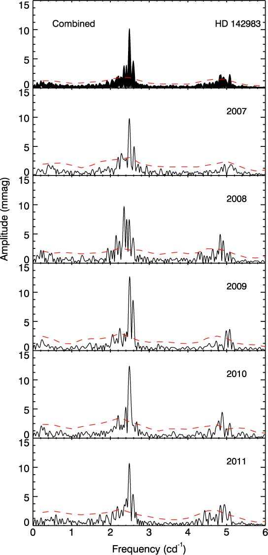
Figure 2. Five-year combined and seasonal amplitude spectra of 48 Lib. The variability is concentrated around two dominant frequency regions, at around 2.49 and 5.00 c d−1. The red dashed lines show the noise levels calculated for every 0.5 c d−1 frequency interval.
The primary frequency generally appears at around 2.49 c d−1 during the 5-yr time interval (Figure 2). However, this frequency shows an unusual change in 2008 by decreasing to 2.35 c d−1. Considering only those changes at around 2.49 c d−1, we realise that it exhibits a beat-like variation in 2007, 2008, 2010, and 2011. We also observe an abnormal increase of about 0.01 c d−1 in 2009 for the same frequency. Analogous with this variability, the frequencies at around 2.17 and 4.95 c d−1 have the same beat-like change over 5 yr. Apart from these, we detect seven frequencies at around 2.20, 2.24, 2.32, 2.37, 2.42, 2.59, and 5.08 c d−1 in the seasonal periodograms. These frequencies are regularly identified in each amplitude spectrum and also observed in the 5-yr combined data set. The variations in 2.42 and 2.59 c d−1 are quite similar, such that they both decrease and show an unusual drop in 2010. Also, the frequencies at 2.20 and 2.32 c d−1 demonstrate a decreasing change between 2007 and 2011. Besides, 2.24 c d−1 displays an increasing frequency profile.
The amplitudes of these frequencies are also variable. The most remarkable changes occur in the amplitudes of 2.49 c d−1 and the seasonal main frequencies. They show a sinusoidal variation with the minimum in 2008 and the maximum in 2010. In addition, the amplitude of 2.20 c d−1 has a decreasing change, whereas the amplitudes of 2.17, 2.32, 2.37, and 2.42 c d−1 exhibit a similar variation with an abnormal increase in 2008.
In addition, we also apply a sliding-window method to all individual data to check every possible frequency and amplitude variations as a function of time. The length of the window is set as 5 d, and it is shifted across the seasonal light curves with a time step of 1 d. In each step, we perform a Fourier analysis by using the LS technique and plot results against the time as in Figure 3. In the figure, the frequencies at around 2.49 and 5.00 c d−1 show up clearly and persistently. However, the rest of the frequencies seem to be more temporary and last in a few days. The variation at around 2.49 c d−1 is always the most dominant structure over the course of 5 yr. Although the frequency of this variation is constant, except in 2008 (f 1 = 2.351 c d−1), it shows daily and seasonal amplitude changes. The frequency at around 5.00 c d−1 is also conspicuous. The most remarkable changes in its amplitude take place in 2008 and 2011. The interesting feature for this frequency is periodic modulations, particularly in 2011, with peak-to-peak period of around 10 d (∼0.1 c d−1). Additionally, as seen from Figure 3, both frequencies are split into two parts (e.g. between the observation days of 8 and 11 in 2011 for the frequency at 2.49 c d−1) and the spacing between these splits is around 0.1 c d−1. This value is quite consistent with the regular spacing seen between the frequencies in the amplitude spectrum.
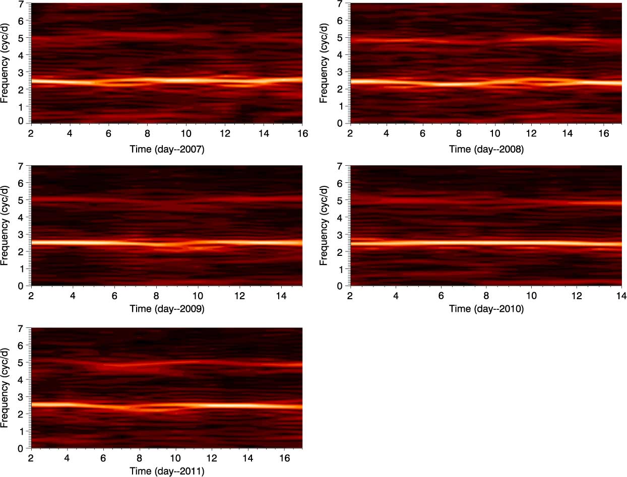
Figure 3. Sliding-window method applied to all individual data to check frequency and amplitude variations as a function of time. The length of the sliding window is 5 d and shifted across the seasonal light curves with the step of 1 d. The mid-points of 5-d sliding windows are used in the x-axis.
4.1. Rotational modulation?
As seen in the frequency spectrum of 48 Lib, the star shows explicit multi-periodicities. However, the structural similarities and constancies of the dominant frequencies at 2.48896(1) and 5.08150(2) c d−1, and the presence of transient frequencies presented in Figure 3 provide a critical evidence that these multi-periodicities are more likely a result of rotation rather than pulsation. Additionally, amplitudes of the frequencies seen in the periodograms display variations which may be a signature of non-uniformly distributed regions on the photosphere or circumstellar material. Such changes are suggested to be related to a change in the size of the spot regions or possible drift in latitude (Balona et al. Reference Balona2011). Also, the frequencies at around 2.17, 2.49, and 4.95 c d−1 exhibit beat-like variations over 5 yr, as discussed in the previous section. This beating effect may also be considered to be originated by inhomogeneous regions in differential rotation (Balona Reference Balona2016). Therefore, the features given as visible harmonic, variable amplitudes, and beating in the light curve make 48 Lib a good candidate that shows rotational modulation. For this reason, the existence of surface or circumstellar inhomogeneities should be considered for this star (Balona Reference Balona, Guzik and Bradley2009).
Such a rotational modulation can be confirmed from the phased light curves of both 5 yr of combined and seasonal data given in Figures 4 and 5. The folded light curve of the combined data is produced by using the data obtained between 2007 and 2011 and using the main frequency given as 2.48896 c d−1. The outliers greater than 3σ are removed from the data. As seen from the figure, the curve has a single sinusoid and clearly asymmetric shape, with major difference in the steepness of the ascending and descending branches: the rising branch is noticeably steeper than the descending one. This type of modulation is attempted to be explained for ξ Per by Ramiaramanantsoa et al. (Reference Ramiaramanantsoa2014). The authors find out the presence of a few co-rotating magnetic bright spots with the same period as the rotation period of the star. In the case of 48 Lib, it is not clear whether such a change can be caused by the presence of a large magnetic spot or multiple spots on the stellar surface.
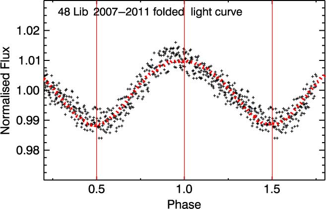
Figure 4. The folded light curve of the entire data set taken between 2007 and 2011. The curve has a single and smooth sinusoidal-like variation with an asymmetry, such that the rising branch is steeper than the descending one. The red curve represents the theoretical light variation produced by a spot model.
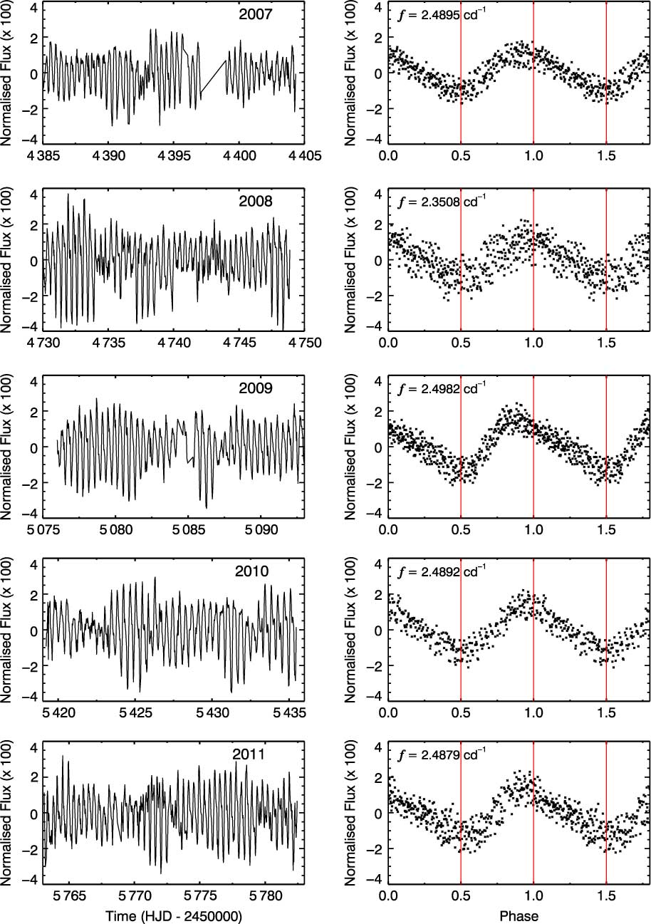
Figure 5. The seasonal and phased light curves. The phased curves are produced by using the main frequency derived from the light curve of that year. The effect of the rotation is seen in each folded light curve.
In order to explain the cause of the asymmetric light modulation seen in the star, the only thing to do is to show how easy it is to obtain a reasonable fit using the simplest possible spot model. In such a model, whose math can be found in Dorren (Reference Cuypers, Balona and Marang1987), we assume that the inclination angle of the star is around 85° (Silaj et al. Reference Silaj2016) and the star has a single circular spot. By entering various spot parameters, we attempt to generate a theoretical light curve that best fits the real observational data. As a result of several trials, we obtain an acceptable fit which explains the curve with the minimum of free parameters. The fit is shown in Figure 4 with the red dashed line, and the related parameters are given in Table 3.
Table 3. The parameters derived from the spot model
As seen from the figure, observational and theoretical data sets are quite compatible with each other (χ2 = 0.0080), which means that the variation seen in the light can be represented by a single-spotted rotation model in the simplest way. However, this by no means is a unique solution, and of course there is not only one solution. Also, the feature causing the light variation does not have to be a single spot. It is possible to make a really good fit by assuming many spots having different lifetimes, sizes, or positions on the star, but this is not very rational since a large number of free parameters have to be adjusted. On the other hand, it does not even have to be a spot. Most likely, it has nothing to do with a sunspot, but is merely some obscuration which is co-rotating with the star. It is actually not possible to know the real solution since there are not enough observations on colour, spectroscopic data, etc., which might constrain the solution.
5. Spectroscopic Observations
In order to investigate the relationship between the photometric and spectroscopic characteristics, spectroscopic observations in the BeSS databaseFootnote a are used.
We examine a number of spectra of 48 Lib in BeSS taken from several telescopes/instruments. For this analysis, we only consider optical spectra having a resolution of 6 000–17 000 and covering the Hα line. Heliocentric velocity corrections are applied to all spectra, and telluric lines occurred due to absorption within the atmosphere are removed by using a reference spectrum that creates a telluric template. Final data are shown in Figure 6.
For the EW measurements of the Hα lines, there are two uncertainties arising from the continuum normalisation and noise caused by telluric lines. The most significant one is related to the continuum normalisation. Therefore, we follow the process described by Jones, Tycner, & Smith (Reference Hubrig, Schöller, Savanov, Yudin, Pogodin, Štefl, Rivinius and Curé2011) and assume that the error of the normalisation is 3%. Then, we carry out the analysis with the SPLOT package of IRAF (noao–onedspec–splot) and measure the EW values.
Figure 6. Spectroscopic observations of 48 Lib obtained from the BeSS database, taken between 2007 and 2011. The spectra show a strong central absorption line surrounded by violet and red emission components, indicating the existence of a circumstellar disk sector in sight of line. The numbers on the right-hand side are Heliocentric Julian Dates (HJD 2 450 000).
In addition, the intensities of the components of the Hα line are evaluated. Since 48 Lib has a double-peaked line profile, the maximum intensities of V and R components are separately measured by subtracting each maximum intensity from the continuum line, and the V/R ratios are calculated from
 \begin{equation}V/R = [F(V) - {F_{\rm{c}}}]/[F(R) - {F_{\rm{c}}}],\end{equation}
where F(V) and F(R) are raw intensities of V and R components, F c is the level of continuum line.
6. Spectroscopic Results
For a better understanding of spectroscopic effects, 20 spectra taken between 2007 and 2011 and a spectrum obtained in 1993 are examined. Only the results covering the period between 2007 and 2011 are presented in order to compare them with the photometric findings derived in the same time interval. The evolution of the emission components and the EW of the Hα profile are shown in Figure 6.
The spectra show a strong and narrow absorption line surrounded by violet (V) and red (R) emission components, indicating the existence of a circumstellar disk. There is also no indication of narrow optical absorption components in any of these spectra. As shown in the figure, the peak intensities vary in time. Although the V component is dominant until HJD 2 454 967, the intensity of R component starts to increase after HJD 2 455 037. Further, they remain almost symmetrical between these dates.
In order to measure the V/R ratio, we calculate peak heights above the zero flux level and present a powerful V/R variation that is likely caused by a one-armed density wave of the disk in Figure 7. Accordingly, we take the opportunity to observe the decreasing branch of a long-term disk variability, which is also presented in detail by Štefl et al. (Reference Štefl, Le Bouquin, Carciofi, Rivinius, Baade and Rantakyrö2012). This decrement is probably about to reach its minimum phase.
Figure 7. The variations in the EW and V/R ratio of the Hα line as well as in the frequency at around 2.24 c d−1.
In addition, we derive the EW values of the Hα profiles and find that these values have a decreasing variation (Figure 7). Also, this decreasing structure seems to contain quasi-periodic cycles with the period of around 2.16(14) yr and the amplitude of 0.76(12) Å.
In the last panel in Figure 7, we display the variation in the frequency at around 2.24 c d−1. As seen in the figure, the variation is correlated with the change seen in the Hα line profile.
7. Discussion
Obtaining more information about the mass loss and disk formation of Be stars is crucial to our understanding of the mechanisms responsible for the Be phenomenon. There are several theories proposed to explain these episodic events. The most discussed assumptions among them are the NRPs and rotational modulations since the majority of Be stars show light and line profile variations. To give some examples, while Walker et al. (Reference Walker2005); Huat et al. (Reference Huat2009), and Neiner et al. (Reference Neiner2012) demonstrate the effectiveness of the NRPs, Degroote et al. (Reference Degroote2009) and Balona (Reference Balona2016) indicate the role of the rotational modulations in Be stars. The appropriateness of these two hypotheses can be evaluated by comparing the line centres and wings of high-resolution spectra, by examining the light curves and the radial velocities of spectral lines, or by monitoring the photometric variability (Sareyan et al. Reference Sareyan1998).
Within this context, we obtain the photometric observations of the star from the STEREO satellite between 2007 and 2011, and sensitively investigate the frequency and amplitude variations. We also look at the Hα emission spectra, taken in the same time interval with that of the photometric observations, from the archives and compare the results.
In order to estimate the rotational period of the star, we use the period–rotation relation, given as
 \begin{equation}{P_{{\rm{rot}}}} = \frac{{50.6{R_ \star }\sin i}}{{v\sin i}}.\end{equation}
For the calculation of v sin i, we derive the critical velocity of the star from  $v_{cr}= \sqrt{2GM_{\star}/3R_{\rm{p}}}$, where $M_\star$ and R p are the mass and the polar radius of the star and are assumed to be 6.07 Mȯ and 3.12 Rȯ, respectively (Silaj et al. Reference Silaj2016). Accordingly, we find the critical velocity to be ∼497 km s−1. Since Silaj et al. (Reference Silaj2016) give that v eq/v cr≈0.80 for 48 Lib, the equatorial velocity (v eq) of the star is calculated as ∼398 km s−1. Also, by assuming that the inclination angle is i = 85° (Silaj et al. Reference Silaj2016), the projected rotational velocity (v sin i) is found to be ∼396 km s−1.
From equation (3) and the values determined above, we estimate a rotational period of ∼2.52 c d−1, which is fairly close to the dominant peak at 2.49 c d−1 derived from the 5-yr combined light curve. It is also obvious from Figure 2 that the amplitude spectra consist of two dominant frequencies at around 2.49 and 5.00 c d−1, and the variations of these two dominant frequencies are almost identical according to Figure 3. This is a strong evidence that there is really only one periodic variation with its harmonic giving rise to the stable light curve shown in Figures 4 and 5.
This 2:1 frequency formation is best explained by Cameron et al. (Reference Cameron2008) with the existence of the dominantly excited prograde modes among the high-order g-modes in Be types. These modes have frequencies of around |m|Ω in the observer’s frame, where |m| is the azimuthal order and Ω is the rotation frequency (Cameron et al. Reference Cameron2008). In a fast rotator, frequencies in the co-rotating frame (fg) of intermediate- to high-order g-modes are quite smaller than |m|Ω. In this case, the frequencies in the observer’s frame are fg−mΩ≈−mΩ, and they produce a group that is close to ≈|m|Ω or that is separated from other groups by ≈|m|Ω (Saio Reference Rivinius, Carciofi and Martayan2014). This property makes the photometric period close to the rotation period or half of it (Cameron et al. Reference Cameron2008).
The observational facts, such as the observed dominant period being consistent with the likely rotation period or a single peak and its harmonics on the amplitude spectrum, seen in 48 Lib, are very similar to the typical characteristics of a rotational variable. In this case, the light variations of 48 Lib can be interpreted as a rotational modulation caused by an inhomogeneous region. The inhomogeneity here refers to a co-rotating spot region, whose existence on or just above the photosphere of A- and B-type stars is theoretically and observationally proved by Cantiello Braithwaite (Reference Cantiello and Braithwaite2011) and Balona (Reference Balona2016), respectively. Also, there are several strong theories suggesting that the periodic variations of Be stars are due to long-lasting co-rotating structures (Balona, Aerts, & Štefl Reference Balona, Aerts and Štefl1999; Balona & Kaye Reference Balona1999; Balona Reference Balona2013b). Similar structure above the photosphere of 48 Lib may be responsible for the main periodicity at 2.49 c d−1. Indeed, Hanuschik & Vrancken (Reference Gutiérrez-Soto, Semaan, Garrido, Baudin, Hubert and Neiner1996) discuss the existence of extremely narrow multiple absorption features in Fe II shell lines that are variable in radial velocity and depth on a short timescale for 48 Lib, and they refer this variation to co-orbiting clumps in the disk or a higher-order distortions in the global density wave.
In this study, the coherence of the photometric data with a simple spot model is investigated in order to reveal the presence of such a non-homogeneous structure on or above the photosphere of 48 Lib. As seen in Figure 4, the model constructed by using only one circular spot represents the 5-yr combined light curve fairly well. However, this result is not a definitive solution. The asymmetry in the phased light curve can be better modelled by using more than one spot or by taking differential rotation into account.
The origin of the photometric obscuration is not clear for the star. However, as given by Spruit (Reference Spruit2002) and Mullan MacDonald (Reference Mullan and MacDonald2005), there is a possibility that this feature may be a result of a magnetic field produced by the Tayler instability in a differentially rotating star. Also, Cantiello Braithwaite (Reference Cantiello and Braithwaite2011) suggest that dynamo action in thin subsurface convection zones in hot stars might generate a magnetic field. In this case, magnetic spots can manifest themselves as hot, bright spots. On the other hand, it is not possible to distinguish between bright and dark spots on the basis of the light curves alone. Moreover, Hubrig et al. (Reference Huat2009) state that rapidly rotating Be stars show magnetic fields of the order of less than 100 G. According to Smith (Reference Smith, Balona, Henrichs and Contel1994), these fields are responsible for the co-rotating structures which arise from mass ejection process through magnetic flaring. In such a process, highly ionised gas is released and trapped in closed magnetic loops. Then, gas escapes along open field lines. It is dragged and accelerated by the rapid rotation of the star. Depending on the rotational velocity, the gas reaches circular orbital speeds at some distance from the star if it is still ionised, and this makes the photometric period close to the rotation period (Balona Reference Balona, Suárez, Garrido, Balona and Christensen-Dalsgaard2013a).
Handling the relation between the mass loss and disk formation in terms of the rotation, it is known that the star needs to be rotating quite close to its critical rotational velocity to eject material into orbit. However, the equatorial velocity of the star is 398 km s−1, and this value is 80% of its critical value calculated as 497 km s−1 (Silaj et al. Reference Silaj2016). Since this percentage is well below the expected value, the rotation alone seems unlikely to be related with mass loss. Therefore, the existence of another mechanism additional to the rotation should be taken into account for 48 Lib. The periodogram of the star contains two low frequencies at 0.109 and 0.199 c d−1, and such frequencies are ascribed to the photometric variability of the long-term outbursts seen in Be stars (Rivinius, Baade, & Carciofi Reference Rivinius, Baade and Štefl2016). On the bases of this, it should be considered that bursts with 10-d period in the star may cause above-stated mass-loss event.
Last but not least, Haubois et al. (Reference Harmanec2012) state that 48 Lib shows a positive correlation between U‒B and B‒V. Although such a behaviour is considered as normal for shell stars (Harmanec Reference Hanuschik and Vrancken1983), it is determined that the colours are also well associated with long-term V/R variation (McDavid et al. Reference McDavid2000). On this basis, Haubois et al. (Reference Harmanec2012) suggest that the colour and magnitude changes observed in the star are linked to the azimuthal structure of the disk governed by the one-armed density wave, seen at different aspect angles over the years.
In parallel with this, the results of the photometric and spectroscopic analysis in this study display a correlation in a way that supports the existence of such structure. Accordingly, the decreasing trends of both EW and V/R ratio are inversely proportional to the change in the frequency seen at around 2.24 c d−1. The minimum phase of the quasi-periodic variation observed in the EW values coincides with the maximum levels of the photometric variations seen at 2.20, 2.42, 2.49, and 4.95 c d−1 as well as those seen in the amplitudes of 2.20 and 2.59 c d−1. Furthermore, the maximum of the quasi-periodic change in EW on around HJD 2 454 600 (2008 season) shows inverse proportion to the changes at 2.17 and 2.37 c d−1, and to the unusual drop in the main frequencies. Also, it inversely varies relative to the amplitudes of 2.49 c d−1 and the main frequencies in the same date, whereas the jumps in the amplitudes of 2.17, 2.32, 2.37, and 2.42 c d−1 have a similar variation. Finally, an inverse correlation is observed between the frequencies at 2.42 and 2.59 c d−1, and the maximum of the quasi-periodic structure occurred on HJD 2 455 450 (2010 season).
Although the STEREO has a shorter seasonal observation duration and collects less data points compared to other space missions, its high-precision data and uninterrupted monitoring ability enable us to measure photometric variations with great accuracy and provide hints about the relation between the photometric and emission line variations. Also, it gives a chance to gain a better understanding of the origin of the dominant peaks and multi-periodicities seen in the star.
Author ORCIDs.
D. Ozuyar, http://orcid.org/0000-0001-8544-0950.
Acknowledgements
We acknowledge assistance from Dr. Vino Sangaralingam, Dr. Gemma Whittaker, Dr. Ibrahim Ozavci, and Zahide Terzioglu in the production of the data used in this study. This work has made use of the BeSS database, operated at LESIA, Observatoire de Meudon, France: http://basebe.obspm.fr. The STEREO Heliospheric Imager was developed by a collaboration that included the Rutherford Appleton Laboratory and the University of Birmingham, both in the United Kingdom, and the Centre Spatial de Lige (CSL), Belgium, and the US Naval Research Laboratory (NRL),Washington DC, USA. The STEREO/SECCHI project is an international consortium of the Naval Research Laboratory (USA), Lockheed Martin Solar and Astrophysics Lab (USA), NASA Goddard Space Flight Center (USA), Rutherford Appleton Laboratory (UK), University of Birmingham (UK), Max-Planck-Institut fr Sonnen-systemforschung (Germany), Centre Spatial de Lige (Belgium), Institut dOptique Thorique et Applique (France), and Institut dAstrophysique Spatiale (France). This research has made use of the simbad database, opened at CDS, Strasbourg, France. This research has also made use of NASA’s Astrophysics Data System.


