1. Introduction
The First Byurakan Survey (FBS), also known as the Markarian survey, was the first systematic objective-prism (OP) survey of the extragalactic sky. This survey was conducted by B. E. Markarian and collaborators from 1965 to 1980. The spectral plates were obtained at the Byurakan Astrophysical Observatory (BAO) using the 1-m Schmidt telescope. Various Kodak (IIF, IIAF, IIaF, and 103aF) emulsions were used during the observations, providing a spectral range of 3 400–6 900 Å. The FBS was originally conducted to search for galaxies with an ultraviolet excess (UVX; Markarian Reference Markarian1967; Markarian et al. Reference Markarian, Lipovetski and Stepanian1989; 1997). Other interesting projects based on the FBS were started in 1987 (known as a second part of the FBS, Abrahamian & Mickaelian Reference Abrahamyan and Mickaelian1996; Mickaelian Reference Mickaelian2008).
The selection and study of faint late-type stars (LTSs, M-type and carbon (C) stars at high Galactic latitudes) were one of the main priorities of the second part of the FBS. All FBS plates have been digitized, resulting in the creation of the Digitized First Byurakan Survey (DFBS) data base (Mickaelian et al. Reference Mickaelian, Nesci and Rossi2007). Its images and spectra are available on the DFBS webFootnote a portal in Trieste. All DFBS plates (∼2 200) were analyzed for LTSs. The second version of the “Revised And Updated Catalogue of the First Byurakan Survey of Late-Type Stars”, containing data for 1 471 M- and C-stars (130 C-type stars, 241 M dwarfs, and 1 100 M-type giants), was generated (Gigoyan et al. Reference Gigoyan, Mickaelian and Kostandyan2019).
The main goal of the present paper is the further exploitation of a Galactic M-giant sample selected on DFBS plates (Gigoyan et al. Reference Gigoyan, Mickaelian and Kostandyan2019), using Gaia EDR3 (Brown et al. Reference Brown, Vallenari and Prusti2021) high accurate photometric and astrometric data including distance values as presented in the catalogue by Bailer-Jones et al. (Reference Bailer-Jones, Rybizki and Fouesneau2021), to estimate important physical parameters and to study the distribution of M-giants in our Galaxy.
Our small paper is structured as follows. In Section 2 we present new additional spectroscopic confirmation for a large number of the FBS selected M-giants. In Section 3 we use modern and large sky-area variability data bases to clarify the variability types of the confirmed M-giants. In Section 4 we exploit the Gaia EDR3 photometric data for these objects to construct color-absolute magnitude diagrams (CaMD) including the Gaia-2MASS-diagram (Lebzelter et al. Reference Lebzelter, Mowlavi and Marigo2018), which is based on Wesenheit functions in the Gaia BP and RP and in 2MASS filters (Strutskie et al. 2006). In Section 5 we focus on 111 FBS Mira-type variables within our sample. Section 6 summarizes our results.
2. New spectroscopic observations
Medium-resolution CCD spectra were obtained for a large fraction of the FBS LTSs at different epochs and with various telescopes. Optical spectra were obtained with the Byurakan Astrophysical Observatory 2.6-m telescope (BAO, Armenia, spectrographs UAGS, ByuFOSC2 and SCORPIO), the Observatory de Haute-Provence (OHP, France) 1.93-m telescope (CARELEC spectrograph), the Cima-Ekar 1.83-m telescope of the Padova Astronomical Observatory (Italy), and the 1.52-m Cassini telescope of the Bologna Astrophysical Observatory (Italy) as described in Gigoyan et al. (Reference Gigoyan, Mickaelian and Kostandyan2019). These spectra allowed to confirm the carbon-rich (C-rich) or oxygen-rich (O-rich) nature of our sample stars.
In Table 1 we give information on telescopes and detectors which were used for FBS LTSs spectroscopy at different epochs.
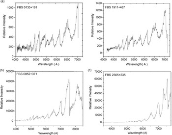
Figure 1(a, b, c) presents consequently the 2.6-m BAO telescope medium-resolution CCD (EEV 42-40) spectra for two M giants FBS 0135 + 191 and FBS 1911 + 487, obtained on November 12, 2018, Loiano 1.52 m telescope spectra for M giant FBS 0852 + 371 (Figure 1b, obtained on 11 February 2007), and Asiago 1.83 m telescope AFOSC spectra for FBS 2305 + 235(Figure 1c, obtained on 6 November 2006) as illustrative examples.
Table 1. Telescopes and detectors used for LTSs spectroscopy

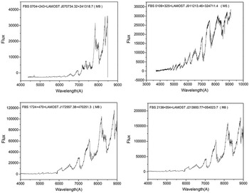
Moderate-resolution CCD spectra for more than 400 FBS LTSs were secured by LAMOST (Large Sky Area Multi-Object Fiber Spectroscopic Telescope) observations (LAMOST DR5, Luo A-L et al. Reference Luo, Zhao and Zhao2019, spectra available on-line at http://dr5.lamost.org/search/). This data set allows an independent verification of our classification, and the O-rich nature could be con- firmed for more than 90% of the FBS M-giants. Figure 2 presents the LAMOST moderate-resolution spectra for four FBS M-giants.
3. Variability study
To determine the variability of the FBS M-giants, we exploit data from two primary sources, namely the Catalina Sky Survey (CSS, second public data release CSDR2, accessed via http://nesssi.cacr.caltech.edu/DataRelease/) and the All-Sky Automated Survey for Supernovae (ASAS-SN, accessed via https://asas-sn.osu.edu/variables/, Shappee et al. Reference Shappee, Prieto and Grupe2014; Kochanek et al. Reference Kochanek, Shappee and Stenek2017; Jayasinghe et al. Reference Jayasinghe, Kochanek and Stenek2018). The CSS comprises two main parts surveying the Northern (Drake et al. Reference Drake, Graham and Djorgovski2014) and the Southern (Drake et al. Reference Drake, Djorgovski and Catelan2017) sky, respectively. Both surveys were analyzed by the Catalina Real-Time Transient Survey (CRTS) in search for optical transient (V < 21.5 mag) phenomena. The ASAS-SN project is an all-sky optical monitoring to a photometric depth V ≤ 17 mag providing variability classification. Consequently, ASAS-SN was used as the primary source for attributing variability types, periods, and amplitudes to the FBS M-giants. For the few objects missing in the ASAS-SN data base, variability parameters were determined from CSDR2 light curves using the VStar-data visualization and analysis tool (Benn Reference Benn2012). Our final sample consists of 690 Semi-Regular (SR)-type, 299 L-type and 111 Mira-type variables.
4. Physical parameters derived from Gaia data
4.1. Gaia EDR3 data
With the advent of Gaia mission (Gaia Collaboration, Prusti et al. Reference Prusti, Bruijne and Brown2016) a new era in astronomical research has started. The Gaia EDR3 (Brown et al. Reference Brown, Vallenari and Prusti2021) contains astrometry, three-band photometry, radial velocities, effective temperatures, and information on astrophysical parameter and variability for approximately 1.8 billion sources brighter than G = 21.0 magnitude.
All FBS M giants were cross-matched with Gaia EDR3 catalogue (CDS VizieR Catalogue I/350/gaiaedr3) sources. The cross-match was carried out using a 5 arcsec aperture around the position of each of our sample stars (the search radius is the same in 2MASS catalogue also). They are relatively bright, so that G–band brightnesses were in the range 7.5 mag < G < 18.0 mag.
4.2. Luminosities and colors for M Giants
The radii and luminosities (in Solar units) of 158 M-giants of our sample (out of 1 100) can be deduced from the Gaia DR2 (Brown et al. Reference Brown, Vallenari and Prusti2018, CDS VizieR Catalogue I/345/gaia2) data base. Luminosities of our target stars range between L = 28.039 L (FBS 0255 + 193 = LAMOST J025756.28 + 193228.5, M1 star) and L = 2024.777 L (FBS 1306 + 385 = LAMOST J130829.62 + 381801.4 = IRAS 13061 + 3834, M6 SR-variable), and effective temperatures lay between 3200 K < Teff < 4 300 K.
A representative sample table for FBS M giants with Gaia EDR3 data is given as Table 2.
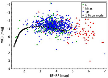
We used the distance information derived from Gaia EDR3 by Bailer-Jones et al. (Reference Bailer-Jones, Rybizki and Fouesneau2021 CDS VizieR Catalogue I/352/gedr3dis) and Gaia EDR3 BP and RP photometry to plot the color-absolute MG magnitude (CaMD) diagram for our complete dataset of 1 054 stars with reliable parallaxes, i.e. uncertainties of less than 20% (Figure 3). Interstellar absorption has been neglected (see below). Different colors denote the various kinds of variables. A stellar evolution track from Marigo et al. (Reference Marigo, Girardi and Bressan2017)Footnote b has been added. The absolute brightness of all our targets correspond to stars on the upper giant branch.

Figure 1. (a) 2.6-m BAO telescope moderate-resolution CCD spectra for two FBS M giants, (b) 1.52-m Loiano telescope spectrum for M giants FBS 0852 + 371, (c) 1.83-m Asiago telescope spectrum for M giant FBS 2305 + 235.

Figure 2. LAMOST moderate-resolution CCD spectra for a sample of FBS M giants.
Table 2. Gaia EDR data for a sample of the FBS M giants.

Notes:IRAS(IRAS Catalogue of Point Sources, Version 2.0, SIMBAD CDS Catalogue II/125/main).
NSVS(Northern Sky Variability Survey, SIMBAD CDS Catalogue J/AJ/128/2965).
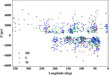
The spatial distribution of the FBS M giant stars in the Milky Way (Galactic longitude vs. vertical height Z above/below the Galactic plane) is plotted in Figure 4. We note that the predominant part of objects is found close to Galactic disk, not more than 5 kpc above or below the Galactic plane. They predominantly represent the Galactic thin and thick disk populations. However, Figure 4 suggests that our sample stars are outside the parts of the disk with the highest interstellar absorption. Therefore, and in the absence of individual reddening values, we decided to neglect corrections for interstellar absorption keeping in mind that the brightness and colors of a few stars may be affected significantly.
4.3 2MASS and Gaia EDR3 photometry
Combining near-infrared (NIR) and Gaia photometric information, Lebzelter et al. (Reference Lebzelter, Mowlavi and Marigo2018) constructed a new diagram as an analysis tool for red giants. For this, they combined Wesenheit functions in the NIR and in the Gaia range. The 2MASS J and Ks NIR Wesenheit function is defined following Soszynski et al. (Reference Soszynski, Udalski and Kubiak2005) as
 \begin{equation}W_{\rm K, J\mbox{-}Ks}=K_{s}-0.686(J-K_s),\end{equation}
whereas the Wesenheit function for Gaia BP and RP magnitudes (Lebzelter et al. Reference Lebzelter, Mowlavi and Marigo2018) is defined as
 \begin{equation}W_{\rm RP,BP\mbox{-}RP}=G_{\rm RP}-1.3(G_{BP}-G_{\rm RP}),\end{equation}
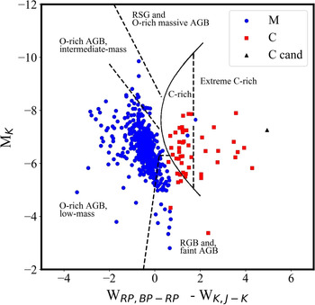
In Figure 5 we show the application of this diagram to spectroscopically confirmed M and C giants with Gaia EDR3 distances (Bailer-Jones et al. Reference Bailer-Jones, Rybizki and Fouesneau2021) within our sample. Lebzelter et al. (Reference Lebzelter, Mowlavi and Marigo2018) constructed this diagram for Large Magellanic Cloud (LMC) long period variables (LPVs) and demonstrated that it allows to identify subgroups among Asymptotic Giant Branch (AGB) stars according to their mass and chemistry. Six distinct groups of red giants with their boundaries had been identified therein (for the definition of the borders of the groups see Table A.1 in Lebzelter et al. Reference Lebzelter, Mowlavi and Marigo2018). These boundaries were shifted according to the distance modulus of the LMC of 18.45 mag (Elgueta et al. Reference Elgueta, Graczyk and Gieren2016). With the help of synthetic stellar population models (based on the TRILEGAL code, Girardi et al. 2005; Marigo et al. Reference Marigo, Girardi and Bressan2017) Lebzelter et al. (Reference Lebzelter, Mowlavi and Marigo2018) showed that these groups correspond to low-mass, intermediate-mass, and massive O-rich AGB stars as well as RSG (red supergiants) and C-stars and extreme C-rich AGB stars, the specific stellar mass range in each of these groups depending on the stellar metallicity (see Figure 3 in Lebzelter et al. Reference Lebzelter, Mowlavi and Marigo2018 for details). The diagram has been explored further by Pastorelli et al. (Reference Pastorelli, Marigo and Girardi2020), with first applications to other stellar systems discussed in Mowlavi et al. (2019) and Pastorelli et al. (in preparation).
Figure 5 nicely confirms the ability of the Gaia-2MASS-diagram to distinguish between M- and C-stars, although there are two objects which, according to our low-resolution spectra, show a spectral type different from the one assumed by its location in that diagram. This is in agreement with findings by Groenewegen et al. (Reference Groenewegen, Nanni and Cioni2020), who detected a few high-mass-loss M-stars in the extreme C-stars region as well. The mass-loss leads to a circumstellar shell, so that M- and C-stars cannot be distinguished reliably.
At low luminosities, several C-stars can be found outside the limits defined by Lebzelter et al. (Reference Lebzelter, Mowlavi and Marigo2018). Such cases can also be seen in synthetic data using a stellar population model (Figure 5 in Lebzelter et al. Reference Lebzelter, Mowlavi and Marigo2018). This makes it likely that the borders defined based on LMC data, lacking stars in this part of the diagram, may need some refinement, in particular in the low luminosity regime.
The majority of the FBS giants occupies the region of low mass, oxygen-rich AGB stars in this diagram. It thus seems likely that the FBS sample primarily consists of stars with M < 2 M Sun. In addition, the diagram reveals a few candidates for intermediate mass AGB stars. The lack of the RSG and massive AGB stars among the sample of the FBS M giants is evident.
As mentioned above, two M giants are found in the right part of the diagram in an area otherwise populated by C-stars (W RP − W Ks > 0.8 mag.), namely FBS 0825 + 626 = IRAS 08258 + 6237, a SR variable with J − K = 2.14, M(G) = −0.61 mag., and FBS 0832-095 = IRAS F08327-0932, Mira-type variable, P = 279 days, J − K s = 1.39, and M(G) = −1.71 mag.
We do not have a spectral class for the object FBS 2216 + 434 = IRAS 22165 + 4326 = V0367 Lac (SR variable: P = 411.59 days, V amplitude 1.08 mag), which we consider as a C-star candidate since it is found in the C-star region of Figure 5 (marked by a black filled triangle).
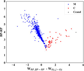
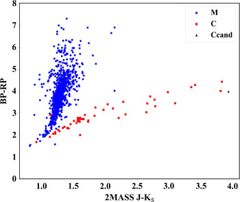
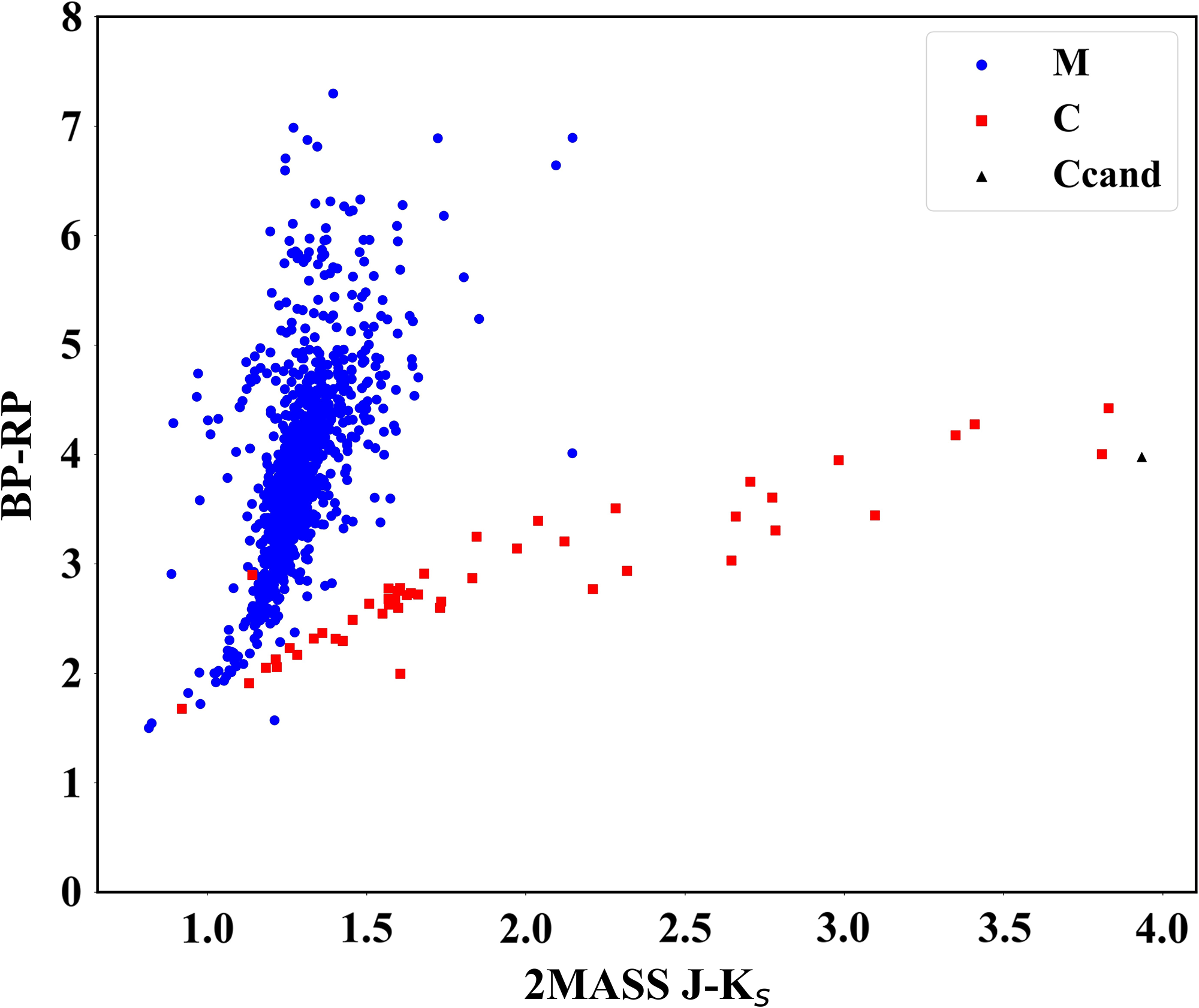
In Figure 6 we present a modified version of this diagram with G BP − G RP on the vertical axis. Figure 7 gives a two-color diagram. Figure 6 seems to allow an even better distinction between the two chemistries than Figure 5. In this case, G BP – G RP appears on both axis since it is part of W RP, BP-RP. Lebzelter et al. (Reference Lebzelter, Mowlavi and Marigo2018) had pointed out that in the Gaia-2MASS-diagram stars get redder from the center to both sides of the horizontal axis, but to the left primarily in G BP − G RP, and to the right in J − K. Since M- and C-stars are sensitive to either of these two colors, the index of two Wesenheit functions allows the above-mentioned distinction. This effect is made even more visible in a diagram like Figure 6 while losing the possibility to separate the stars according to their mass. In this sense, Figures 5 and 6 may form a complementary combination for the analysis of AGB populations. However, in both cases misclassification of a few stars cannot be avoided. The index on the horizontal axis in Figure 6 is reddening free so that any interstellar reddening affects the vertical axis only, while this is not the case in Figure 7. The narrowness of the two branches can be seen as an indicator for low reddening of our stars, as we had assumed due to their location outside the Galactic disk, but that would likely affect the analysis of a population with a higher level of interstellar reddening. A further exploration of these preliminary results is planned.

Figure 3. M (G) vs. BP-RP diagram of FBS M-giants. A 1 M⊙ evolutionary track (Marigo et al. Reference Marigo, Girardi and Bressan2017) has been added with small black crosses. The evolutionary track includes the AGB, but dust has not been considered.

Figure 4. Galactic distribution of the FBS M giants reported in this paper. The symbols are the same as in Figure 3.

Figure 5. WRP,BP-RP -WKs, J-Ks versus MKs diagram for FBS M and C giants. Approximate boundaries of regions (a), (b), (c), and (d) identified for LMC stars in Figure 1 and 3 by Lebzelter et al. (Reference Lebzelter, Mowlavi and Marigo2018) have been reconstructed and shifted from LMC distance. The candidate C star FBS 2216 + 434 is noted as a black filled triangle.

Figure 6. W RP − W Ks versus Gaia EDR3 BP-RP color for FBS M and C giants. The point where C and M stars split is around W RP – W Ks ∼ 0.8 mag. and BP-RP = 2.3 mag. Objects are getting redder both towards lower and higher values of the W RP, BP-RP – W Ks, J-Ks index. The symbols are the same as in Fig. 5.
4.4. Kinematic study
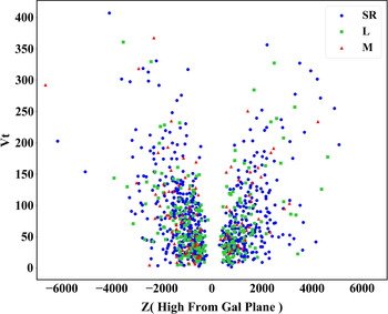
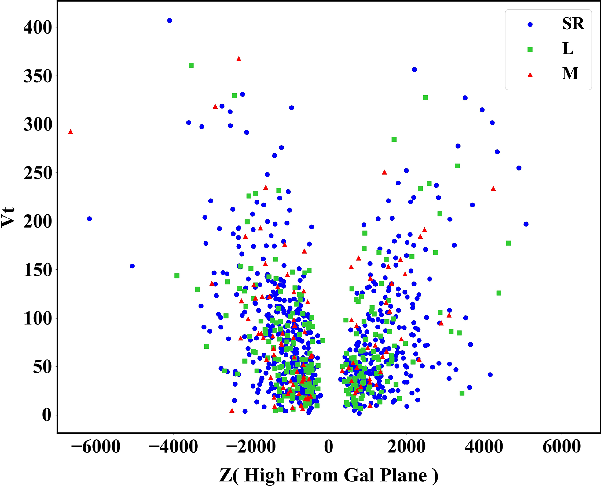
Radial velocity data are available for 134 out of 1 100 objects. We use here tangential velocities for all FBS objects. Tangential velocities are well suited to distinguish various populations within the Milky Way, in particular the Galactic thick disk, thin disk, and halo populations because of their different kinematics and age (Babusiaux et al. Reference Babusiaux, van Leeuween and Barstow2018). Tangential velocity computation is based on Gaia EDR3 proper motion and parallax data (see details of the computation in Babuisiaux et al. 2018). Figure 8 illustrates the tangential velocities (V t) versus height above/below the Galactic plane for these FBS M giants. Only for 9 objects V t > 300 km s−1 was found. Babusiaux et al. (Reference Babusiaux, van Leeuween and Barstow2018) distinguish, based on HRD and kinematics from Gaia data, thin disk (V t < 40 km s−1), thick disk (60 < V t < 150 km s−1), and halo (V t > 200 km s−1) objects (Figures 20 and 21 of Babusiaux et al. Reference Babusiaux, van Leeuween and Barstow2018). The predominant part of the FBS M giants belong to the thick disk (near 37% of the objects) and thin disk (41% of objects), adopting these criteria for tangential velocities. Only 12% of the FBS M giants can be assumed as halo population objects.
5. Mira variables within our sample
Among the 1 100 FBS M giants, 111 are classified as Mira variables in the ASAS-SN variability database, all of them being spectroscopically confirmed M-stars. Mira variables are AGB stars that show large amplitude (>2.5 mag in the V-band) variability with typical periods of 100–1 000 days. Both, oxygen-rich and carbon-rich Miras obey distinguished P-L relations (Feast et al. Reference Feast, Glass, Whitelock and Catchpole1989) useable for independent distance calibration (Whitelock et al. Reference Whitelock, Feast and van Leeuwen2008). Given that the mean period of a population of O-rich Miras correlates with age, Grady et al. (Reference Grady, Belokurov and Evans2019, Reference Grady, Belokurov and Evans2020) used these variables for studying age gradients throughout the Milky Way and the transition in ages between disc and halo O-rich Miras as well as for comparing the relative ages of different Galactic populations as a function of Galactocentric distance. They assembled the largest sample of M-type Miras so far, using data from the Catalina Surveys (Northern and Southern) and ASAS-SN (∼2 400 O-rich Miras). The period of a Mira increases with increasing luminosity, and hence depends on its mass and its evolutionary status along the AGB. Thus, longer period Miras tend to correspond to higher masses (see Figure 6 in Hughes & Wood Reference Hughes and Wood1990).
Periods for the 111 FBS M-type Miras have been taken from the ASAS-SN data base. All these periods were checked by visual inspection of the light curves and corrected in some cases. Figure 9 presents the distribution of periods. It peaks between 250 and 300 days with hardly any Miras showing periods above 400 days. This suggests that the FBS Mira sample mainly consists of low mass AGB stars with a typical mass around 1 M8. The result is consistent with the conclusions derived from photometry in Sect. 4.3 and suggests an age range between 3 and 10 Gyrs for our sample Miras.

Figure 9. Period distribution of the 111 FBS M-type Mira variables based on ASAS-SN periods validated by the authors.
6. Discussion and conclusion
In this paper we explored the sample of 1 100 relatively bright, spectroscopically confirmed M- and a small number of C-giants from the second edition of the FBS LTS catalogue including various kinds of long period variables. For this study, we cross-correlated our sample with the data bases from Gaia EDR3, the Catalina Sky Survey (CSS), 2MASS, and All-Sky Automated Survey for Supernovae (ASAS-SN). This allowed characterizing the FBS sample in more detail. One of our main goals was to study the location of the spectroscopical- ly confirmed FBS O-rich and C-rich giants in the new diagnostic diagram presented by Lebzelter et al. (Reference Lebzelter, Mowlavi and Marigo2018) combining 2MASS infrared and Gaia EDR3 optical photometry. Our conclusions can be summarized as follows:
-
(a) Most of our FBS sample stars are found at typical distances of 1 kpc above or below the plane. Therefore, the sample is only mildly affected by interstellar reddening. No difference between Miras and SRVs has been found.
-
(b) Spectroscopically confirmed FBS O-rich and C-rich giants show the same separation in the Gaia-2MASS-diagram according to their chemistry as the LPVs of the LMC originally used to construct this diagnostic tool, providing another confirmation of its reliability. The discrimination between O-rich and C-rich objects becomes even more visible when using the WRP, BP-RP – WKs, J-Ks versus Gaia BP-RP colour or 2MASS J-Ks versus BP-RP. This offers the opportunity to use the difference of Wesenheit indices WRP, BP-RP – WKs, J-Ks also for chemistry classification in samples with unknown distances while losing the ability of the Gaia-2MASS diagram to separate the stars according to mass.
-
(c) Using multiple diagnostic tools, namely the Gaia-2MASS diagram, the tangential velocity from Gaia, the location and distribution of the sample relative to the Galactic plane, and the period distribution, we consistently found that the FBS giants predominantly consist of low-mass AGB or RGB stars, which are members of the Galactic thin and thick disk population with very few halo candidates.
Our study illustrated the possibilities to investigate samples of red giants using the data bases from large surveys and the Gaia-2MASS diagram. Analogue studies have been carried out on spectroscopically confirmed faint M and C stars noted as periodic variables at high Galactic latitudes in the Catalina (Drake et al. Reference Drake, Graham and Djorgovski2014, Reference Drake, Djorgovski and Catelan2017) and LINEAR (Palaversa et al. Reference Palaversa, Ivezic and Eyer2013) catalogues (Gigoyan et al. Reference Gigoyan, Kostandyan and Gigoyan2021). A dominant fraction of those M- and C-giants belongs to the Halo and to arms of the Sagittarius dwarf galaxy. The results will be published soon. The full list of the 1100 FBS LTSs (M and C giants) including various astrometric and photometric data from the Gaia EDR3, 2MASS, ASAS-SN, and CSS catalogues is available on request by mailing Gigoyan K. S.
Acknowledgements
This research was made possible using the ASAS-SN and Catalina Sky Survey variability data bases. We used the LAMOST telescope spectra. The LAMOST is a National Major Scientific project build by the Chinese Academy of Sciences. This work has made use of data from the European Space Agency (ESA) mission Gaia (https://cosmos.esa.int/gaia), processed by the Gaia Data Processing and Analysis Consortium (DPAC, https://www.cosmos.esa.int/web/gaia/dpac.consoortium). This research has made use of the SIMBAD database, operated at CDS, Strasbourg, France. This publication makes use of data products from the Two Micron All Sky Survey, which is a joint project of the University of Massachusetts and the Infrared Processing and Analysis Center/California Institute of Technology, funded by the National Aeronautics and Space Administration and the National Science Foundation.
K. S. G. acknowledges Victor Ambartsumian International Science Prize International Steering Committe for supporting this project. We thank Dr. Marigo for providing a stellar evolution track used in Figure 3.