


1. Introduction
The Square Kilometre Array (SKA) is a large international collaboration, with the goal of building the world’s largest and most powerful radio telescope. The first phase of the SKA (‘SKA1’) will begin operations in the early 2020s and will comprise two separate arrays: SKA1-Low, which will consist of around 130 000 low-frequency dipoles in Western Australia, and SKA1-Mid, which will be composed of  $\sim$200 dishes in the Karoo region of South Africa (Dewdney et al. Reference Dewdney, Turner, Braun, Santander-Vela, Waterson and Tan2016; Braun Reference Braun2017). The second phase, SKA2, will be an order of magnitude larger in collecting area than SKA1 and will take shape in the late 2020s.
The science case for the SKA is extensive and diverse: the SKA will deliver spectacular new datasets that are expected to transform our understanding of astronomy, ranging from planet formation to the high-redshift Universe (Bourke et al. Reference Bourke2015). However, the SKA will also be a powerful machine for probing the frontiers of fundamental physics. To fully understand the SKA’s potential in this area, a focused workshop on ‘Fundamental Physics with the Square Kilometre Array’Footnote a was held in Mauritius in May 2017, in which radio astronomers and theoretical physicists came together to jointly consider ways in which the SKA can test and explore fundamental physics.
This paper is not a proceedings from this workshop, but rather is a white paper that fully develops the themes explored. The goal is to set out four broad directions for pursuing new physics with the SKA and to serve as a bridging document accessible for both the physics and astronomy communities. In Section 2, we consider cosmic dawn and reionisation, in Section 3 discuss strong gravity and pulsars, in Section 4 we examine cosmology and dark energy, and in Section 5 we review dark matter (DM) and astroparticle physics. In each of these sections, we introduce the topic, set out the key science questions, and describe the proposed experiments with the SKA.
2. Cosmic dawn and reionisation
Cosmic dawn represents the epoch of formation of the first stars and galaxies that eventually contributed to the reionisation of the Universe. This period is potentially observable through the 21-cm spin-flip transition of neutral hydrogen, redshifted to radio frequencies. In this section, we provide an overview of the ways in which we can use upcoming SKA observations of cosmic dawn and of the epoch of reionisation (EoR) to place constraints on fundamental physics. These include the possible effects of warm dark matter (WDM) on the 21-cm power spectrum during cosmic dawn, variations of fundamental constants such as the fine structure constant, measurements of the lensing convergence power spectrum, constraints on inflationary models, and cosmic microwave background (CMB) spectral distortions and dissipation processes. We describe foreseeable challenges in the detection and isolation of the fundamental physics parameters from the observations of cosmic dawn and reionisation, possible ways towards overcoming them through effective isolation of the astrophysics, synergies with other probes, and foreground removal techniques.
2.1. Introduction
Cosmologists seek to use the Universe as an experiment from which to learn about new physics. There has already been considerable success in extracting fundamental physics from the CMB and from large-scale structure (LSS) measurements from large galaxy surveys. These CMB and LSS observations cover only a small fraction of the total observable Universe, both in terms of cosmic history and observable volume. A promising new technique for providing observations over the redshift range  $z=3-27$ is by measurements of the 21-cm hyperfine line of neutral hydrogen, which can be observed redshifted to radio frequencies detectable by the SKA (Koopmans et al. Reference Koopmans2015).
Since hydrogen is ubiquitous in intergalactic space, 21-cm observations offer a route to mapping out fluctuations in density, which contain information about cosmological parameters. As the 21-cm line is affected by various types of radiation, observing it gives a way to detect and study some of the first astrophysical objects, including stars and black holes (BHs). Once detected, the 21-cm signal might also provide information about the high-redshift Universe that can constrain other physics, such as the effects of WDM, annihilation or scattering of DM, the variation of fundamental constants, and possibly also tests of inflationary models (Pritchard et al. Reference Pritchard2015).
These are exciting times for cosmic dawn and reionisation, as the pathfinder experiments Low Frequency Array (LOFAR) (Patil et al. Reference Patil2017), Murchison Widefield Array (MWA) (Dillon et al. Reference Dillon2015), Precision Array for Probing the Epoch of Reioniization (PAPER) (Ali et al. Reference Ali2015), and Hydrogen Epoch of Reionisation Array (HERA) (DeBoer et al. Reference DeBoer2017) have begun to collect data and set upper limits on the 21-cm power spectrum, while Experiment to Detect the Epoch of Reionization Signature (EDGES) has reported a tentative detection (Bowman et al. Reference Bowman, Rogers, Monsalve, Mozdzen and Mahesh2018). It is likely that in the next few years, the cosmological 21-cm signal will open a new window into a previously unobserved period of cosmic history.
The rest of this section is organised as follows. In Section 2.2, we present a brief overview of the theory and observations related to cosmic dawn and the EoR, and the various physical processes that influence the magnitude of the signal from these epochs. We summarise the status of observations in the field, including the upper limits to date from various experiments. We also provide a brief overview of the upcoming observations and modelling of the reionisation epoch. In Section 2.3, we review aspects of fundamental physics that can be probed with the SKA, and in Section 2.4 we discuss some of the challenges to doing this. We provide a summary in Section 2.5.
2.2. Cosmic dawn and reionisation: Theory and observations
2.2.1 Overview of the 21-cm signal
The 21-cm line of neutral hydrogen corresponds to the transition between the singlet and triplet hyperfine levels of its electronic ground state, resulting from the interaction of proton and electron spins. The resulting transition has a rest frame frequency of 1.4 GHz, that is, a wavelength of 21 cm. The electric dipole transition between the ground and excited hyperfine levels is forbidden due to parity; the lowest order transition occurs via a magnetic dipole, owing to which the triplet level has a vacuum lifetime of  $\simeq\! 11 \ {\rm Myr}$. Due to this long lifetime, the dominant channels for the decay of the excited levels are either non-radiative (atomic collisions; Allison & Dalgarno Reference Allison and Dalgarno1969; Zygelman Reference Zygelman2005) or depend on the existing radiation field (stimulated emission by CMB photons, or optical pumping by UV photons; Wouthuysen Reference Wouthuysen1952; Field Reference Field1958). This makes the relative population of the hyperfine levels a sensitive probe of the thermal state and density of the high-redshift intergalactic medium (IGM) and of early sources of ultraviolet radiation (Sunyaev & Zeldovich Reference Sunyaev and Zeldovich1975; Hogan & Rees Reference Hogan and Rees1979; Madau et al. Reference Madau, Meiksin and Rees1997).
Radio observations of this line are frequently used to map the velocity of neutral hydrogen (H i) gas in the Milky Way or in nearby galaxies, but currently it has not been detected in emission at redshifts  $z>1$. When considering the 21-cm line as a cosmological probe, it is standard to describe the measured intensity in terms of a brightness temperatureFootnote b and to consider the observed brightness temperature relative to some background source, typically either the CMB or a radio-bright point source. For cosmology, it is most useful to consider the case of the CMB backlight, for which the 21-cm signal will then take the form of a spectral distortion over the whole sky.
The observable quantity is the brightness temperature,  $\delta T_{\rm b}$, of the 21-cm line against the CMB, which is set by radiative transfer through H i regions. The brightness temperature of 21-cm radiation can be expressed as
 $$
\begin{align}
\nonumber\\[-10pt] \delta T_{b}(\nu) &= \frac{T_{s} -
T_{\gamma}}{1+z} (1 - e^{-\tau_{\nu_0}}) \nonumber \\[3pt]
& \approx 27 x_{\rm H {i}} (1+\delta_{b}) \left(\frac{H}{dv_r/dr + H}\right)
\left(1 - \frac{T_{\rm cmb}}{T_{s}} \right) \nonumber \\[3pt]
& \times \left( \frac{1+z}{10} \frac{0.15}{\Omega_{\rm m}
h^2}\right)^{1/2} \left( \frac{\Omega_b h^2}{0.023} \right) {\rm
mK},
\label{eqn1}\end{align}
$$
$$
\begin{align}
\nonumber\\[-10pt] \delta T_{b}(\nu) &= \frac{T_{s} -
T_{\gamma}}{1+z} (1 - e^{-\tau_{\nu_0}}) \nonumber \\[3pt]
& \approx 27 x_{\rm H {i}} (1+\delta_{b}) \left(\frac{H}{dv_r/dr + H}\right)
\left(1 - \frac{T_{\rm cmb}}{T_{s}} \right) \nonumber \\[3pt]
& \times \left( \frac{1+z}{10} \frac{0.15}{\Omega_{\rm m}
h^2}\right)^{1/2} \left( \frac{\Omega_b h^2}{0.023} \right) {\rm
mK},
\label{eqn1}\end{align}
$$ where  $T_s$ is the gas spin temperature, $\tau_{\nu_0}$ is the optical depth at the 21-cm frequency $\nu_0$, $x_{\rm H {i}}$ is the neutral hydrogen fraction of the IGM,
  $\delta_{b}({\bf x},
z) \equiv \rho/\bar{\rho} - 1$ is the evolved (Eulerian) density contrast of baryons, H(z) is the Hubble parameter,
$\delta_{b}({\bf x},
z) \equiv \rho/\bar{\rho} - 1$ is the evolved (Eulerian) density contrast of baryons, H(z) is the Hubble parameter,  $dv_r/dr$ is the co-moving gradient of the line-of-sight component of the peculiar velocity, and all quantities are evaluated at redshift $z=\nu_0/\nu - 1$; $\Omega_b$ is the present-day baryon density and h is the present-day Hubble factor. Therefore, the brightness temperature of the 21-cm line is very sensitive to the spin temperature of the gas and to the CMB temperature (Mesinger et al. Reference Mesinger, Furlanetto and Cen2011).
The 21-cm line is a unique window into cosmological epochs at which the Universe is dominantly composed of neutral hydrogen atoms. These encompass the period from cosmological recombination (a redshift of  $z = 1100$, or a proper time of $0.38 \ {\rm Myr}$ after the Big Bang) to the end of the reionisation era (a redshift of $z \simeq 6$, or a proper time of $\simeq 1.2 \ {\rm Gyr}$ after the Big Bang). Except for the last epoch, the rest of this period is unconstrained by current observations and is fertile ground for exploration with new observations. There are several processes that contribute to the evolution of the brightness temperature of the 21-cm radiation. Observations of the brightness temperature, either through direct imaging or statistical measures of its fluctuations, can then inform us about the physical state of the neutral gas and the nature of its perturbations (Koopmans et al. Reference Koopmans2015).
1. During the period from  $z \simeq 1100$ to $z \simeq 200$, the gas temperature is kept close to that of the CMB by Thomson scattering of residual free electrons (Chluba & Sunyaev Reference Chluba and Sunyaev2012). Atomic collisions and optical pumping by Lyman- $\alpha$ photons from the epoch of cosmological recombination can lead to a small but non-negligible brightness temperature in the 21-cm line (Fialkov & Loeb Reference Fialkov and Loeb2013; Breysse et al. Reference Breysse, Ali-Haïmoud and Hirata2018).
2. The epoch from  $z \simeq 200$ to $z\simeq30$ is known as the Dark Ages; through this period, the CMB temperature and the gas temperature differ substantially, and atomic collisions are sufficiently fast to set the spin temperature to the latter and lead to a 21-cm signal at a detectable level. The amplitude of the signal is set by the linear evolution of fluctuations on large scales (Loeb & Zaldarriaga Reference Loeb and Zaldarriaga2004; Lewis & Challinor Reference Lewis and Challinor2007) and the bulk flows that set the baryonic Jeans scale (Tseliakhovich & Hirata Reference Tseliakhovich and Hirata2010; Ali-Haïmoud et al. Reference Ali-Haïmoud, Meerburg and Yuan2014). If detected, the 21-cm signal from this epoch would be the ultimate probe of primordial cosmological fluctuations. Assuming cosmic variance limits, the 21-cm signal could probe extremely faint inflationary gravitational wave (GW) backgrounds (down to tensor-to-scalar ratios of
  $r \sim
10^{-9}$; Masui & Pen Reference Masui and Pen2010; Book et al. Reference Book, Kamionkowski and Schmidt2012) and low levels of primordial non-gaussianities (down to parameters
$r \sim
10^{-9}$; Masui & Pen Reference Masui and Pen2010; Book et al. Reference Book, Kamionkowski and Schmidt2012) and low levels of primordial non-gaussianities (down to parameters  $f_{\rm NL} \simeq
0.03$; Cooray Reference Cooray2006; Pillepich et al. Reference Pillepich, Porciani and Matarrese2007; Joudaki et al. Reference Joudaki, Doré, Ferramacho, Kaplinghat and Santos2011; Muñoz et al. Reference Muñoz, Ali-Haïmoud and Kamionkowski2015). Due to the low frequencies of the signal from this epoch, the observational prospects are not promising in the short to medium term.
$f_{\rm NL} \simeq
0.03$; Cooray Reference Cooray2006; Pillepich et al. Reference Pillepich, Porciani and Matarrese2007; Joudaki et al. Reference Joudaki, Doré, Ferramacho, Kaplinghat and Santos2011; Muñoz et al. Reference Muñoz, Ali-Haïmoud and Kamionkowski2015). Due to the low frequencies of the signal from this epoch, the observational prospects are not promising in the short to medium term.
3. The period covering redshifts  $z \simeq 30-15$ is called the cosmic dawn epoch, owing to the birth of the first stars (in sufficient numbers to affect 21-cm observations). The radiation emitted by these first sources significantly changes the nature of the mean and fluctuating 21-cm signal due to two main reasons: (i) optical pumping of the hyperfine levels due to Lyman- $\alpha$ photons, known as the Wouthuysen–Field effect, which serves to couple the spin temperature of the gas to the ambient Lyman- $\alpha$ radiation (Hirata Reference Hirata2006), and (ii) heating of the gas by X-rays (Furlanetto Reference Furlanetto2006; Pritchard & Furlanetto Reference Pritchard and Furlanetto2007; Fialkov et al. Reference Fialkov, Barkana and Visbal2014). In addition, non-linear structure formation (Ahn et al. Reference Ahn, Shapiro, Alvarez, Iliev, Martel and Ryu2006; Kuhlen et al. Reference Kuhlen, Madau and Montgomery2006) and baryonic bulk flows (Visbal et al. Reference Visbal, Barkana, Fialkov, Tseliakhovich and Hirata2012; McQuinn & O’Leary Reference McQuinn and O’Leary2012; Fialkov et al. Reference Fialkov, Barkana, Visbal, Tseliakhovich and Hirata2013) imprint their effects on the signal. Primordial magnetic fields can also lead to features in the cosmological 21-cm signal during these epochs (Shiraishi et al. Reference Shiraishi, Tashiro and Ichiki2014).
4. Finally, during the epochs covered by  $z \simeq 15-6$, the ionising photons from the radiation sources lead to the permeation of HII regions, and the mean signal drops, reaching close to zero as reionisation is completed.
Significant progress has been made in condensing these rich astrophysical effects into simple semi-analytical prescriptions that capture the large-scale features of the 21-cm signal during this period (Furlanetto et al. Reference Furlanetto, Zaldarriaga and Hernquist2004a,b; Mesinger & Furlanetto Reference Mesinger and Furlanetto2007; Mesinger et al. Reference Mesinger, Furlanetto and Cen2011; Visbal et al. Reference Visbal, Barkana, Fialkov, Tseliakhovich and Hirata2012). For a fiducial model described by Mesinger et al. (Reference Mesinger, Furlanetto and Cen2011) and developed with the publicly available code 21CMFAST, the various evolutionary stages of the signal are illustrated in Figure 1. The terms in the figure denote the spin temperature of the gas  $T_s$, the CMB temperature $T_{\gamma}$, and the gas kinetic temperature $T_K$; the figure illustrates astrophysical effects on the signal that include decoupling from the CMB, the Wouthuysen–Field coupling, and X-ray heating. Figure 2 shows the wide range of possibilities for the sky-averaged signal (‘the 21-cm global signal’). Its characteristic structure of peaks and troughs encodes information about global cosmic events. Cohen et al. (Reference Cohen, Fialkov, Barkana and Lotem2017) discussed 193 different combinations of astrophysical parameters, illustrating the great current uncertainty in the predicted 21-cm signal.

Figure 1. Evolution of spin temperature  $T_s$, gas temperature $T_K$, and CMB temperature $T_{\gamma}$. This figure is taken from Mesinger et al. (Reference Mesinger, Furlanetto and Cen2011).
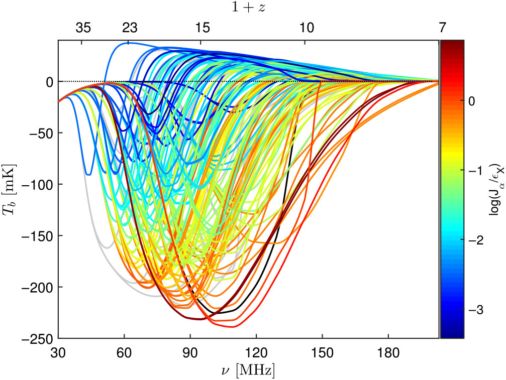
Figure 2. The 21-cm global signal as a function of redshift, for the 193 different astrophysical models discussed in Cohen et al. (Reference Cohen, Fialkov, Barkana and Lotem2017). The colour (see the colour bar on the right) indicates the ratio between the Ly $\alpha$ intensity (in units of erg s–1 cm–2 Hz–1 sr–1) and the X-ray heating rate (in units of eV s–1 baryon–1) at the minimum point. Grey curves indicate cases with $\tau>0.09$, and a non-excluded case with the X-ray efficiency of X-ray sources set to zero; these cases are all excluded from the colour bar range. Figure taken from Cohen et al. (Reference Cohen, Fialkov, Barkana and Lotem2017).
The most robust way of probing cosmology with the brightness temperature may be redshift-space distortions (RSDs); (Barkana & Loeb 2005 a; Furlanetto et al. Reference Furlanetto2009); see however Shapiro et al. (Reference Shapiro, Mao, Iliev, Mellema, Datta, Ahn and Koda2013) and Fialkov et al. (Reference Fialkov, Barkana and Cohen2015). Alternatively, a discussion of the bispectrum is provided by Saiyad Ali et al. (Reference Saiyad Ali, Bharadwaj and Pandey2006). More futuristic possibilities include probing extremely weak primordial magnetic fields ( $\sim\! 10^{-21} \ {\rm G}$ scaled to $z=0$) using their breaking of the line-of-sight symmetry of the 21-cm power spectrum (Venumadhav et al. Reference Venumadhav, Oklopˇci´c, Gluscevic, Mishra and Hirata2017) and inflationary GWs through the circular polarisation of the 21-cm line (Hirata et al. Reference Hirata, Mishra and Venumadhav2018; Mishra & Hirata Reference Mishra and Hirata2018).
2.2.2. Status of 21-cm experiments
Observational attempts to detect the cosmological 21-cm signal have made significant progress in the last few years, with upper limits from interferometers beginning to make contact with the space of plausible models. Broadly speaking, there are two classes of 21-cm experiments: those attempting to measure the sky-averaged ‘global’ 21-cm signal and those attempting to measure the 21-cm brightness temperature fluctuations. A natural comparison is to the CMB where some experiments target either spectral distortions to the CMB blackbody (BB), while others measure CMB anisotropies.
Experiments targeting the global signal include EDGES (Bowman et al. Reference Bowman, Morales and Hewitt2008), SARAS (Patra et al. Reference Patra, Subrahmanyan, Raghunathan and Udaya Shankar2013), LEDAFootnote c, SCI-HI (Voytek et al. Reference Voytek, Natarajan, Jáuregui García, Peterson and López- Cruz2014), and a proposed lunar experiment DARE (Burns et al. Reference Burns2012). To detect the 21-cm global signal, in principle, only a single radio dipole is necessary, as its large beam will average over fluctuations to probe the averaged all sky signal. For these experiments, raw sensitivity is typically not the limiting factor; the main challenges are twofold—ensuring absolute calibration of the dipole and removing foregrounds.
In Bowman et al. (Reference Bowman, Morales and Hewitt2008), EDGES reported the first lower limit on the duration of reionisation by searching for a sharp step in the 21-cm global signal, which is, in principle, distinguishable from the smooth foregrounds (Pritchard & Loeb Reference Pritchard and Loeb2010). More sophisticated techniques have been developed based upon forward modelling the signal, foregrounds, and instrument response in a Bayesian framework and prospects appear to be good (Harker et al. Reference Harker, Pritchard, Burns and Bowman2012).
Recently, EDGES reported a detection of the 21-cm global signal in absorption at a frequency of 78 MHz, corresponding to the redshift  $z \sim 17$ (Bowman et al. Reference Bowman, Rogers, Monsalve, Mozdzen and Mahesh2018). The absorption profile was flattened, with an amplitude about twice that predicted by several current models. The signal amplitude could possibly be evidence of interactions between (a subcomponent of) DM and baryons (e.g., Barkana Reference Barkana2018; Barkana et al. Reference Barkana2018; Muñoz & Loeb Reference Muñoz and Loeb2018), which may have led to cooling of the IGM prior to reionisation. Further investigation, as well as independent confirmation from other facilities, would lead to exciting prospects for constraining fundamental physics.
In parallel, several new radio interferometers—LOFAR, PAPER, MWA, HERA—are targeting the spatial fluctuations of the 21-cm signal, due to the ionised bubbles during cosmic reionisation as well as Lyman- $\alpha$ fluctuations (Barkana & Loeb Reference Barkana and Loeb2005b) and X-ray heating fluctuations (Pritchard & Furlanetto Reference Pritchard and Furlanetto2007) during cosmic dawn. These telescopes take different approaches to their design, which gives each different pros and cons. LOFAR in the Netherlands is a general purpose observatory with a moderately dense core and long baselines (in the case of the international stations, extending as far as Ireland). The MWA in Western Australia is composed of 256 tiles of 16 antennas distributed within about 1-km baselines. PAPER (now complete) was composed of 128 dipoles mounted in a small dish and focused on technological development and testing of redundant calibration. HERA in South Africa will be a hexagonal array of 330 $\times$ 14 m dishes and, like PAPER, aims to exploit redundant calibration.
These experiments have begun setting upper limits on the 21-cm power spectrum that are summarised in Figure 3. At present, the best constraints are about two orders of magnitude above the expected 21-cm power spectrum. However, as noted earlier, there is considerable uncertainty in these predictions, and in the case of an unheated IGM, a much larger signal can be produced. Pober et al. (Reference Pober2015) interpreted now-retracted upper limits from Ali et al. (Reference Ali2015) as a constraint on the IGM temperature, ruling out an entirely unheated Universe at  $z=8.4$. The current upper limits typically represent only a few tens of hours of integration time, compared to the $\sim\!1000$ h needed for the desired sensitivity. Systematic effects, especially instrumental calibration, currently limit the amount of integration time that can be usefully reduced. Overcoming these limitations is the major goal of all these experiments and steady progress is being made.
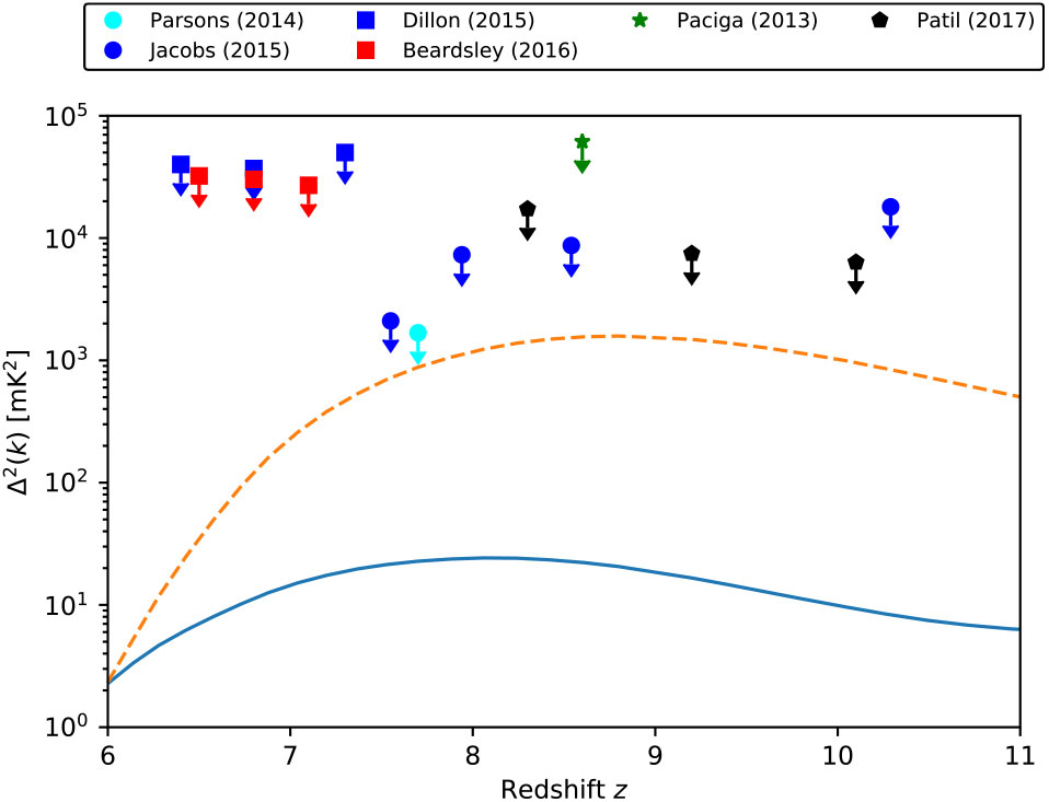
Figure 3. Summary of current constraints on the 21-cm power spectrum as a function of redshift. Since constraints are actually a function of both redshift and wavenumber k, only the best constraint for each experiment has been plotted. Here are plotted results for GMRT (Paciga et al. Reference Paciga2013), PAPER32 (Parsons et al. Reference Parsons2014; Jacobs et al. Reference Jacobs2015), MWA128 (Dillon et al. Reference Dillon2015; Beardsley et al. Reference Beardsley2016), and LOFAR (Patil et al. Reference Patil2017). Two comparison 21-cm signals calculated using 21CMFAST are shown to give a sense of the target range—one with fiducial values (solid blue curve) and a second with negligible heating (dashed orange curve).
2.3. Fundamental physics from the EoR
In the previous section, we listed the main astrophysical and cosmological processes that contribute to the brightness temperature evolution of the 21-cm signal and the status of the EoR 21-cm experiments. In this section, we provide glimpses into the details of some of the important constraints on fundamental physics that may be garnered from the EoR and cosmic dawn.
2.3.1. Cosmology from the EoR
A key advantage of 21-cm observations is that they open up a new epoch of cosmological volume containing many linear modes of the density field, which can greatly increase the precision of cosmological parameter constraints. Typically, cosmology enters into the 21-cm signal through its dependence on the density field, so that the 21-cm signal can be viewed as a biased tracer in a similar way to low-redshift galaxy surveys. The challenge is that obtaining fundamental physics from the 21-cm signal requires disentangling the ‘gastrophysics’—the effect of galaxies and other astrophysical sources on the hydrogen gas—from the signature of physics. This is not an easy challenge, since the effect of astrophysics is typically dominant over that of fundamental physics effects, which are often subtle and desired to be measured at high precision. At this moment in time, our understanding of the nuances of both the 21-cm signal and the observations is still relatively limited, but there are reasons for some optimism.
Broadly speaking, there are several routes to fundamental physics from the 21-cm signal:
1. Treat the 21-cm signal as a biased tracer of the density field, and via joint analysis, constrain cosmological parameters.
2. Look for the direct signature of energy injection by exotic processes in the 21-cm signal, which is sensitive to the cosmic thermal history.
3. The clustering of ionised regions or heating will reflect the underlying clustering of galaxies, and so will contain information about the density field, for example, non-gaussianity signatures or the lack of small-scale structure due to WDM.
4. Line-of-sight effects, such as weak lensing or the integrated Sachs–Wolfe (ISW) effect, where the 21-cm signal is primarily just a diffuse background source.
5. Look for unique signatures of fundamental physics, for example, the variation of the fine structure constant, which do not depend in detail upon fluctuations in the 21-cm brightness.
21-cm observations may also be useful in breaking degeneracies present in other datasets (Kern et al. Reference Kern, Liu, Parsons, Mesinger and Greig2017). For example, measurements of the reionisation history may allow the inference of the optical depth to the CMB, breaking a degeneracy with neutrino mass (Liu et al. Reference Liu, Pritchard, Allison, Parsons, Seljak and Sherwin2016).
2.3.2. Exotic energy injection
As discussed in Section 2.2.1, the 21-cm signal is sensitive to the underlying gas temperature through the 21-cm spin temperature. This makes the 21-cm line a rather unique probe of the thermal history of the Universe during the EoR and the cosmic dawn. Provided that the IGM temperature is not too much larger than the CMB temperature (so that the  $1 -
T_{\rm CMB}/T_s$ term retains its dependence on
$1 -
T_{\rm CMB}/T_s$ term retains its dependence on  $T_s$), we can use the Universe as a calorimeter to search for energy injection from a wide range of processes. Distinguishing different sources of heat will depend upon them having unique signatures in how that energy is deposited spatially or temporally.
After thermal decoupling at  $z\sim150$, the gas temperature is expected to cool adiabatically, with a phase of X-ray heating from galaxies warming the gas, before the photoionisation heating during reionisation raises the temperature to $\sim\!10^4{\,\rm K}$ (e.g., Furlanetto Reference Furlanetto2006; McQuinn & O’Leary Reference McQuinn and O’Leary2012). There is considerable uncertainty in these latter stages, which depend upon poorly known properties of the galaxies and the cosmic star formation history.
Many authors have put forward possible sources of more exotic heating, including annihilating DM (e.g., Furlanetto et al. Reference Furlanetto, Oh and Pierpaoli2006; Valdés et al. Reference Valdés, Evoli, Mesinger, Ferrara and Yoshida2013), evaporating primordial black holes (PBHs) (Clark et al. Reference Clark, Dutta, Gao, Strigari and Watson2017; Mack & Wesley Reference Mack and Wesley2008), cosmic string wakes (Brandenberger et al. Reference Brandenberger, Danos, Hernández and Holder2010), and many more. In many cases, these might be distinguished from X-ray heating by (a) occurring before significant galaxy formation has occurred or (b) by depositing energy more uniformly than would be expected from galaxy clustering. Incorporation of DM annihilation models into simulations of the 21-cm signal suggests that plausible DM candidates might be ruled out by future 21-cm observations (Valdés et al. Reference Valdés, Evoli, Mesinger, Ferrara and Yoshida2013). Ultimately, the physics of how DM annihilation produces and deposits energy as heating or ionisation is complex and requires consideration of the decay products and their propagation from the decay site into the IGM (Schön et al. Reference Schön, Mack, Avram, Wyithe and Barberio2015).
Note that DM candidates may modify the thermal history through their effect on the distribution of galaxies too, as discussed in the next section.
2.3.3. Warm DM effects
WDM is an important alternative to the standard cold dark matter (CDM) candidate. Although there have been a series of studies on the constraints on the mass of the WDM, a large parameter space is still unexplored and is possible in principle. These existing constraints include the lower limit on the mass of a thermal WDM particle ( $m_{X}\geq 2.3\, \rm{keV}$) from Milky Way satellites (Polisensky & Ricotti Reference Polisensky and Ricotti2011) and from Lyman- $\alpha$ forest data (Narayanan et al. Reference Narayanan, Spergel, Davé and Ma2000; Viel Reference Viel, Williams, Shu and Menard2005; Viel et al. Reference Viel, Becker, Bolton, Haehnelt, Rauch and Sargent2008).
A possible effect of WDM during the reionisation and cosmic dawn epochs is distinguishable from both the mean brightness temperature and the power spectra. The key processes that are altered in the WDM model are the Wouthysen–Field coupling, the X-ray heating, and the reionisation effects described in Section 2.2.1. This is because the WDM can delay the first object formation, so the absorption features in the  $\delta T_{b}$ evolution could be strongly delayed or suppressed. In addition, the X-ray heating process, which relies on the X-rays from the first generation of sources, as well as the Lyman- $\alpha$ emissivity, can be also affected due to the delayed first objects (see also Figure 7 of Pritchard & Loeb Reference Pritchard and Loeb2012). Of course, the magnitude of the effects depends on the scale of interest. Finally, reionisation is also affected because the WDM can delay the reionisation process, and therefore affect the ionisation fraction of the Universe at redshift $\sim\!10$ (Figures 8 and 9 of Barkana et al. Reference Barkana, Haiman and Ostriker2001).
Examples of the effects of WDM models on the spin temperature of the gas will be discussed in Section 5.2.3. For the case of WDM, the spin temperature,  $T_{\rm S}$, stays near the CMB temperature, $T_{\gamma}$, at redshift $z>100$. The absorption trough occurs due to the fact that at a later stage, the X-ray heating rate surpasses the adiabatic cooling. Initially, the mean collapse fraction in WDM models is lower than in CDM models, but it grows more rapidly in the heating of gas.
The mean brightness temperature as a function of redshift (frequency) for such WDM models with  $m_{\text{X}}=2,\,3,\,4\,\text{keV}$, respectively, is explored by Sitwell et al. (Reference Sitwell, Mesinger, Ma and Sigurdson2014) and elaborated on in Section 5.2.3. It is shown that if the WDM mass is below the limit $m_{\text{X}}<10\,\text{keV}$, it can substantially change the mean evolution of $\overline{T}_{\rm b}(z)$.
In addition to the mean temperature evolution, Sitwell et al. (Reference Sitwell, Mesinger, Ma and Sigurdson2014) also explored the power spectrum of WDM models, and showed a three-peak structure in  $k=0.08
$ and
$k=0.08
$ and  $k=0.18 \, \text{Mpc}^{-1}$ modes, which are associated with inhomogeneities in the Wouthuysen–Field coupling coefficient $x_{\alpha}$, the kinetic temperature $T_{\rm K}$, and the ionisation fraction $x_{\text{HI}}$, from high to low redshifts. As discussed in detail in Section 5.2.3, the power at these specific modes can be boosted, depending upon the mass of the WDM particle.
These variations in the mean temperature and fluctuations can be measured and tested using current interferometric radio telescopes. Mesinger et al. (Reference Mesinger, Ewall-Wice and Hewitt2014) and Sitwell et al. (Reference Sitwell, Mesinger, Ma and Sigurdson2014) showed forecasts for the 1- $\sigma$ thermal noise levels for 2 000 h of observation time for the MWAFootnote d, the HERAFootnote e, and for SKA1-Low. On the other hand, there are major uncertainties in the evolution of high-redshift star formation (in low-mass halos in particular), with a potentially complex history due to various astrophysical feedback mechanisms [including photo-heating, Lyman–Werner radiation (photons capable of dissociating molecular hydrogen), and supernova feedback; the latter includes hydrodynamic and radiative feedback as well as metal enrichment]. The estimates do indicate that next-generation radio observations may be able to test the excess power in the power spectra of brightness temperature for $m_{\text{X}}<10 \, \text{keV}$ models over a wide range of redshifts. The SKA, in particular, will provide a unique prospect of measuring the mean brightness temperature and the 21-cm power spectrum out to $z\simeq 20$. However, distinguishing WDM from CDM will require a clear separation from possible astrophysical effects.
2.3.4. Measuring the fine structure constant with the SKA using the 21-cm line
The standard model of particle physics fails to explain the values of some fundamental ‘constants’, like the mass ratio of the electron to the proton, the fine structure constant, etc. (see e.g., Uzan Reference Uzan2011). Dirac (Reference Dirac1937) hypothesised that these constants might change in space as well as in time. Studies using the optical spectra of distant quasars indicated, controversially, the existence of temporal (e.g., Webb et al. Reference Webb, Murphy, Flambaum, Dzuba, Barrow, Churchill, Prochaska and Wolfe2001) and spatial (e.g., Webb et al. Reference Webb, King, Murphy, Flambaum, Carswell and Bainbridge2011) variations in the fine structure constant,  $\alpha$ (but see also Srianand et al. (Reference Srianand, Chand, Petitjean and Aracil2004) and the more recent results of Murphy et al. (Reference Murphy, Malec and Prochaska2016) suggesting no significant cosmological variations. However, these results may be in tension with terrestrial experiments using optical atomic clocks, which set a very stringent limit on the temporal variation of $\alpha$ (Rosenband et al. Reference Rosenband2008). Investigation along these lines has great significance to our understanding of gravitation through the underlying equivalence principle (Shao & Wex 2016), as well as fundamental (scalar) fields and cosmology (Damour et al. Reference Damour, Piazza and Veneziano2002). It could also provide an intriguing clue to the outstanding ‘cosmological constant problem’ (Parkinson et al. Reference Parkinson, Bassett and Barrow2004).
In the case that  $\alpha$ varies as a function of time (e.g., as a cosmologically evolving scalar field), the evolution could be non-monotonic in general. Therefore, it would be greatly beneficial if we could measure $\alpha$ at various redshifts. The quasar spectra and optical atomic clocks mentioned previously only probe $\alpha$ at moderate redshifts, $0.5 \lesssim z \lesssim 3.5$ and $z \simeq 0$, respectively. Hence, reionisation and cosmic dawn provide an interesting avenue to probe the possibility of a varying $\alpha$ at large z. Because of its high resolution in radio spectral lines, SKA1-Low has good prospects to use them (e.g., lines from Hi and the OH radical) to determine $\alpha$ (Curran Reference Curran, Lobanov, Zensus, Cesarsky and Diamond2007; SKA Science Working Group 2011). The covered redshifts for SKA1-Low will be, for example,
  $z
\lesssim 13$ for the Hi 21-cm absorption and
$z
\lesssim 13$ for the Hi 21-cm absorption and  $z \lesssim 16$ for the ground-state 18 -cm OH absorption (Curran et al. Reference Curran, Kanekar and Darling2004). Khatri & Wandelt (Reference Khatri and Wandelt2007) proposed another method to measure $\alpha$, through the 21-cm absorption of CMB photons. They found that the 21-cm signal is very sensitive to variations in $\alpha$, such that a change of 1% in $\alpha$ modifies the mean brightness temperature decrement of the CMB due to 21-cm absorption by $\gtrsim5\%$ over the redshift range
  $30 \lesssim z
\lesssim 50$. It also affects, as a characteristic function of the redshift z, the angular power spectrum of fluctuations in the 21-cm absorption; however, the measurement of the angular power spectrum at these redshifts (corresponding to the Dark Ages) would require lower frequency observations than those from the SKA. In summary, constraints on the variation of
$30 \lesssim z
\lesssim 50$. It also affects, as a characteristic function of the redshift z, the angular power spectrum of fluctuations in the 21-cm absorption; however, the measurement of the angular power spectrum at these redshifts (corresponding to the Dark Ages) would require lower frequency observations than those from the SKA. In summary, constraints on the variation of  $\alpha$ at various redshifts will significantly advance our basic understanding of nature and might provide clues to new physics beyond the standard model (Uzan Reference Uzan2011).
2.3.5. Cosmic shear and the EoR
Important information on the distribution of matter is encoded by weak lensing of the 21-cm signal along the line of sight to the EoR (Pritchard et al. Reference Pritchard2015). Zahn & Zaldarriaga (Reference Zahn and Zaldarriaga2006) and Metcalf & White (Reference Metcalf and White2009) showed that a large area survey at SKA sensitivity might have the potential to determine the lensing convergence power spectrum via the non-gaussianity of 21-cm maps. It remains to be seen over what area SKA-Low surveys might have the sensitivity to measure cosmic shear, but the proposed deep EoR survey over 100 deg $^2$ should be sufficient. This would measure how DM is distributed in a representative patch of sky, something feasible only with galaxy lensing towards unusually large galaxy clusters. This might offer the chance to match luminous matter with overall mass, thereby constraining the DM paradigm.
The convergence power spectrum can be estimated using the Fourier space quadratic estimator technique of Hu (Reference Hu2001), originally developed for lensing data on the CMB and expanded to 3D observables, that is, the 21-cm intensity field  $I(\theta,z)$ discussed by Zahn & Zaldarriaga (Reference Zahn and Zaldarriaga2006) and Metcalf & White (Reference Metcalf and White2009).
The convergence estimator and the corresponding lensing reconstruction noise are derived under the assumption that there is a gaussian distribution in temperature. This will not completely hold for the EoR, since reionisation introduces considerable non-gaussianity, but acts as a reasonable approximation.
The benefit of 21-cm lensing is that one can combine data from multiple redshift slices. In Fourier space, fluctuations in temperature (brightness) are separated into wave vectors normal to the sightline  $\mathbf{k_\perp}=\mathbf{l}/r$, with r the angular diameter distance to the source redshift, and a discretised parallel wave vector
  $k_\parallel =
2\pi j/\mathcal{L}$, where
$k_\parallel =
2\pi j/\mathcal{L}$, where  $\mathcal{L}$ is the depth of the volume observed. Considering modes with different values of j to be orthogonal, an optimal estimator results from combining the estimators from separate j modes without any mixing. The reconstruction noise of 3D lensing is then (Zahn & Zaldarriaga Reference Zahn and Zaldarriaga2006):
 $$
\begin{equation}
N(L,\nu) =\left[\sum_{j=1}^{j_{\rm max}}
\frac{1}{L^2}\int \frac{d^2\ell}{(2\pi)^2} \frac{[\mathbf{l} \cdot \mathbf{L}
C_{\ell,j}+\mathbf{L} \cdot (\mathbf{L}-\mathbf{l})
C_{|\ell-L|,j}]^2}{2 C^{\rm tot}_{\ell,j}C^{\rm
tot}_{|\mathbf{l}-\mathbf{L}|,j}}\right]^{-1}.
\label{eqn2}
\end{equation}
$$
$$
\begin{equation}
N(L,\nu) =\left[\sum_{j=1}^{j_{\rm max}}
\frac{1}{L^2}\int \frac{d^2\ell}{(2\pi)^2} \frac{[\mathbf{l} \cdot \mathbf{L}
C_{\ell,j}+\mathbf{L} \cdot (\mathbf{L}-\mathbf{l})
C_{|\ell-L|,j}]^2}{2 C^{\rm tot}_{\ell,j}C^{\rm
tot}_{|\mathbf{l}-\mathbf{L}|,j}}\right]^{-1}.
\label{eqn2}
\end{equation}
$$ Here,  $C^{\rm tot}_{\ell,j}=C_{\ell,j}+C^{\rm N}_\ell$, where $C_{\ell,j}=[\bar{T}(z)]^2P_{\ell,j}$ with $\bar{T}(z)$ the mean observed brightness temperature at redshift z due to the mean density of HI and $P_{\ell,j}$ is the associated power spectrum of DM (Zahn & Zaldarriaga Reference Zahn and Zaldarriaga2006).
Figure 4 gives a sense of the sensitivity to the convergence power spectrum that might be achieved with SKA-Low after 1 000 h integration on a 20-deg $^2$ field. It should be feasible to measure the signal associated with lensing over a range of angular scales. Increasing the survey area would allow access to large angular scales, where the signal-to-noise is the greatest. This measurement would be significantly improved with the larger sensitivity of SKA2 (Romeo et al. Reference Romeo, Metcalf and Pourtsidou2018). For redshifts after reionisation, the power spectrum of weak lensing should be better measured using SKA-Mid and the 21-cm intensity mapping (IM) approach discussed above, but covering a much wider sky area (Pourtsidou & Metcalf Reference Pourtsidou and Metcalf2014).
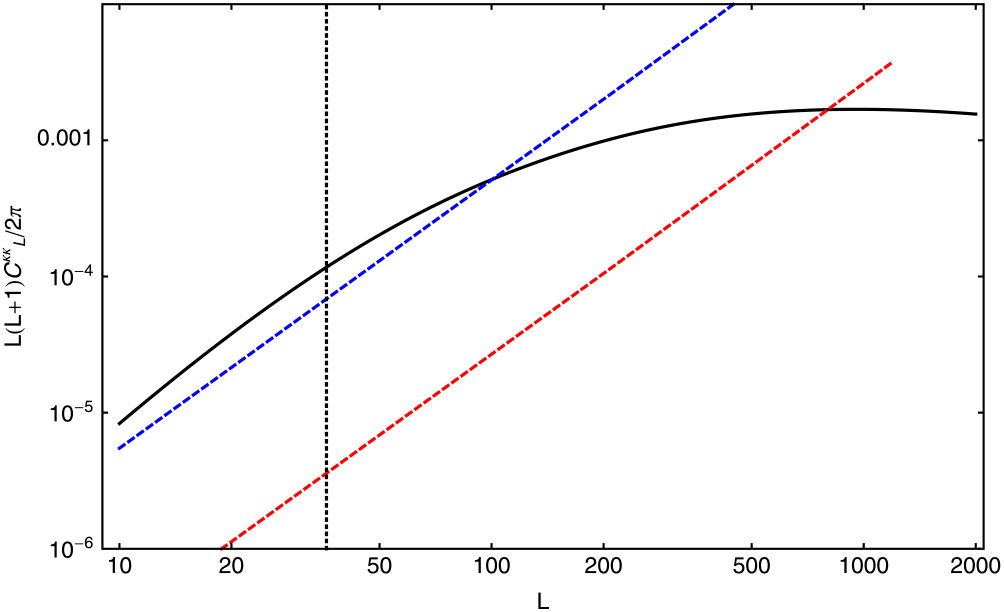
Figure 4. The solid black line shows the power spectrum of the lensing convergence field,  $C^{\kappa \kappa}_L$, for sources at $z=8$; dashed lines indicate the noise associated with lensing reconstruction, $N_L$. The blue dashed line is for SKA1-Low with ten 8-MHz frequency bins around $z=8$, covering redshifts from $z \simeq 6.5$ to $z \simeq 11$. The red dashed line is the same but for SKA2-Low. The vertical line represents an estimate of the lowest possible value of L accessible in a 5-by-5 degree field. Regions where noise curves fall below $C^{\kappa \kappa}_L$ indicate cases for which the typical fluctuations in the lensing deflection should be recoverable in a map. Figure taken from Pritchard et al. (Reference Pritchard2015).
2.3.6. Integrated Sachs–Wolfe effect
In Section 2.2.1, we provided an overview of the 21-cm brightness temperature fluctuation and its dependence on cosmological and astrophysical parameters. While we have thus far focused on high redshifts, it will be possible to use 21-cm measurements from after reionisation in order to obtain constraints on various cosmological models. In this case, the 21-cm emission comes from hydrogen atoms within galaxies. The intensity (or equivalently temperature) fluctuations can be mapped on large scales, without resolving individual galaxies; this measurement is known as 21-cm IM. In this section, we consider using the post-reionisation power spectrum of the temperature brightness measured by the SKA, and the cross-correlation of SKA IM measurements with SKA galaxy number counts, in order to detect the ISW effect. As examples of measurements that can be obtained with this observable, we look at the IM constraining power to test statistical anisotropy and inflationary models.
Raccanelli et al. (Reference Raccanelli, Kovetz, Dai and Kamionkowski2016a) presented a study on using the cross-correlation of 21-cm surveys at high redshifts with galaxy number counts; the formalism and methodology is described in that paper. The use of 21-cm radiation instead of the (standard) CMB can provide a confirmation of the detection of the ISW effect, which will be detected by several instruments at different frequencies at the time, and hence influenced by different systematics.
The ISW effect (Sachs & Wolfe Reference Sachs and Wolfe1967; Crittenden & Turok Reference Crittenden and Turok1996; Nishizawa Reference Nishizawa2014) is a gravitational redshift due to the time evolution of the gravitational potential when photons traverse underdensities and overdensities in their journey from the last scattering surface to the observer. This effect produces temperature fluctuations that are proportional to the derivative of gravitational potentials.
The ISW effect has been detected (Nolta et al. Reference Nolta2004; Pietrobon et al. Reference Pietrobon, Balbi and Marinucci2006; Ho et al. Reference Ho, Hirata, Padmanabhan, Seljak and Bahcall2008; Giannantonio et al. Reference Giannantonio, Scranton, Crittenden, Nichol, Boughn, Myers and Richards2008a; Raccanelli et al. Reference Raccanelli, Bonaldi, Negrello, Matarrese, Tormen and de Zotti2008; Giannantonio et al. Reference Giannantonio, Crittenden, Nichol and Ross2012; Planck Collaboration et al. 2014a; Reference Collaboration2016f) through cross-correlation of CMB maps at GHz frequencies with galaxy surveys. It has also been used to constrain cosmological parameters (Giannantonio et al. Reference Giannantonio, Scranton, Crittenden, Nichol, Boughn, Myers and Richards2008b; Massardi et al. Reference Massardi, Bonaldi, Negrello, Ricciardi, Raccanelli and de Zotti2010; Bertacca et al. Reference Bertacca, Raccanelli, Piattella, Pietrobon, Bartolo, Matarrese and Giannantonio2011; Raccanelli et al. Reference Raccanelli2015).
Similar to the CMB, the 21-cm background at high redshifts, described by the brightness temperature fluctuation in Section 2.2.1, will also experience an ISW effect from the evolution of gravitational potential wells (see Figure 5). The dominant signal present is that of unscattered CMB photons, and therefore its late-time ISW signature is highly correlated with the signature at the peak CMB frequencies. A complementary measurement at 21-cm frequencies is promising as it represents an independent detection of the ISW effect, measured with different instruments and contaminated by different foregrounds. As the 21-cm background is set to be observed across a vast redshift range by upcoming experiments, there should be ample signal-to-noise for this detection. The ISW effect on those CMB photons that do interact with the neutral hydrogen clouds at high redshifts provide a source of observable signal. Assuming the CMB fluctuations can be efficiently subtracted from the 21-cm maps, this signal can potentially be detected in the data as well.

Figure 5. Illustration: Radiative transfer of CMB photons through neutral hydrogen gas clouds induces fluctuations at 21-cm frequencies (due to absorption or emission, depending on the relative temperatures of the IGM and the CMB). The majority of the signal is comprised of unscattered CMB photons at the Rayleigh-Jeans tail of its BB spectrum. These photons later undergo line-of-sight blue- or red-shifting as they travel through the evolving gravitational potential wells. Figure taken from Raccanelli et al. (Reference Raccanelli, Kovetz, Dai and Kamionkowski2016a).
To detect the ISW effect, one would cross-correlate the brightness temperature maps with galaxy catalogues. In the case when the photons are unscattered, the detection is more difficult to obtain. The detection depends on a series of parameters of the 21-cm detecting instrument, such as the observing time, the frequency bandwidth, the fractional area coverage, and the length of the baseline. The results weakly depend on the details of the galaxy survey used. Different surveys give slightly different results, but do not lead to a dramatic change in the overall signal-to-noise ratio. Targeting specific redshift ranges and objects could help. The main advantage for detecting the ISW effect is due to the large area of the sky covered. If we assume the standard general relativity (GR) and  $\Lambda$ cold dark matter ( $\Lambda$CDM) cosmology, the ISW effect is mostly important during the late-time accelerated phase, so low-redshift galaxies are to be targeted. The use of a tomographic analysis in the galaxy catalogue and the combination of different surveys (see e.g., Giannantonio et al. Reference Giannantonio, Scranton, Crittenden, Nichol, Boughn, Myers and Richards2008a; Bertacca et al. Reference Bertacca, Raccanelli, Piattella, Pietrobon, Bartolo, Matarrese and Giannantonio2011) can improve the detection of the signal in the case of the LSS-CMB correlation.
2.3.7. Statistical anisotropy
Most inflationary models predict the primordial cosmological perturbations to be statistically homogeneous and isotropic. CMB observations, however, indicate a possible departure from statistical isotropy in the form of a dipolar power modulation at large angular scales. A 3 $\sigma$ detection of the dipolar power asymmetry, that is, a different power spectrum in two opposite poles of the sky, was reported based on analysis of the off-diagonal components of Please provide the expansion for “WMAP” if necessary. angular correlations of CMB anisotropies with Wilkinson Microwave Anisotropy Probe and Planck data on large scales (Hansen et al. Reference Hansen, Banday and Gorski2004; Gordon et al. Reference Gordon, Hu, Huterer and Crawford2005; Eriksen et al. Reference Eriksen, Banday, Gorski, Hansen and Lilje2007; Gordon Reference Gordon2007; Planck Collaboration et al. Reference Collaboration2014b; Akrami et al. Reference Akrami, Fantaye, Shafieloo, Eriksen and Hansen2014; Planck Collaboration et al. Reference Collaboration2016e; Planck Collaboration et al. Reference Collaboration2016e,c; Aiola et al. Reference Aiola, Wang, Kosowsky, Kahniashvili and Firouzjahi2015). The distribution of quasars at later times was, however, studied by Hirata (Reference Hirata2009), and showed an agreement with statistical isotropy on much smaller angular scales.
A significant detection of deviation from statistical isotropy or homogeneity would be inconsistent with some of the simplest models of inflation, making it necessary to postulate new physics, such as non-scalar degrees of freedom. It would, moreover, open a window into the physics of the early Universe, thus shedding light upon the primordial degrees of freedom responsible for inflation.
The off-diagonal components of the angular power spectrum of the 21-cm intensity fluctuations can be used to test this power asymmetry, as discussed in detail by Shiraishi et al. (Reference Shiraishi, Muñoz, Kamionkowski and Raccanelli2016). One can also constrain the rotational invariance of the Universe using the power spectrum of 21-cm fluctuations at the end of the Dark Ages. The potential ability to access small angular scales gives one the opportunity to distinguish the dipolar asymmetry generated by a variable spectral index, below the intermediate scales at which this vanishes. One can compute the angular power spectrum of 21-cm fluctuations sourced by the dipolar and quadrupolar asymmetries, including several non-trivial scale dependencies motivated by theories and observations. By the simple application of an estimator for CMB rotational asymmetry (Pullen & Kamionkowski Reference Pullen and Kamionkowski2007; Hanson & Lewis Reference Hanson and Lewis2009), we can forecast how well 21-cm surveys can constrain departures from rotational invariance. Results for dipolar and quadrupolar asymmetries, for different models and surveys, are discussed by Shiraishi et al. (Reference Shiraishi, Muñoz, Kamionkowski and Raccanelli2016), who show that the planned SKA may not reach the same precision as future CMB experiments in this regard; however, an enhanced SKA instrument could provide the best measurements of statistical anisotropy, for both the dipolar and quadrupolar asymmetry.
The SKA could, though, provide some constraining power for asymmetry parameters since 21-cm measurements have different systematics and come from an entirely different observable compared to the CMB. Moreover, 21-cm surveys provide an independent probe of broken rotational invariance, and as such, would help in disentangling potential biases present in previous CMB experiments.
2.3.8. Tests of inflation
Measurements of IM from SKA can be used to constrain inflationary models via limits on the matter power spectrum, in particular the spectral index and its ‘running’.
Single-field slow-roll inflation models predict a nearly scale-invariant power spectrum of perturbations, as observed at the scales accessible to current cosmological experiments. This spectrum is slightly red, showing a non-zero tilt. A direct consequence of this tilt are non-vanishing runnings of the spectral indices,  $\alpha_s=\mathrm d n_s/\mathrm
d\log k$, and
$\alpha_s=\mathrm d n_s/\mathrm
d\log k$, and  $\beta_s=\mathrm d\alpha_s/\mathrm d\log k$, which in the minimal inflationary scenario should reach absolute values of $10^{-3}$ and $10^{-5}$, respectively. This is of particular importance for PBH production in the early Universe, where a significant increase in power is required at the scale corresponding to the PBH mass, which is of order $k \sim 10^5$ Mpc–1 for solar mass PBHs (Green & Liddle Reference Green and Liddle1999; Carr Reference Carr2005). It has been argued that a value of the second running $\beta_s = 0.03$, within 1 $\sigma$ of the Planck results, can generate fluctuations leading to the formation of $30\, {\rm M}_{\odot}$ PBHs if extrapolated to the smallest scales (Carr et al. Reference Carr, Kühnel and Sandstad2016).
The measurements of 21-cm IM can be used to measure these runnings. A fully covered 1-kilometre-baseline interferometer, observing the EoR, will be able to measure the running  $\alpha_s$ with $10^{-3}$ precision, enough to test the inflationary prediction. However, to reach the sensitivity required for a measurement of $\beta_s\sim 10^{-5}$, a Dark Ages interferometer, with a baseline of $\sim\! 300$ km, will be required. Detailed analyses of 21-cm IM experiments forecasts for this (including comparisons with CMB and galaxy surveys) measurements have been made recently (Muñoz et al. Reference Muñoz, Kovetz, Raccanelli, Kamionkowski and Silk2017; Pourtsidou et al. Reference Pourtsidou, Bacon and Crittenden2017; Sekiguchi et al. Reference Sekiguchi, Takahashi, Tashiro and Yokoyama2018).
2.3.9. Free-free emission from cosmological reionisation
As we know, the CMB emerges from the thermalisation epoch, at  $z \sim
10^{6}-10^{7}$, with a BB spectrum thanks to the combined effect of Compton scattering and photon emission/absorption processes (double Compton and bremsstrahlung) in the cosmic plasma, which, at early times, are able to re-establish full thermal equilibrium in the presence of arbitrary levels of perturbing processes. Subsequently, the efficiency of the scattering and above radiative processes decreases because of the expansion of the Universe and the consequent combined reduction of particle number densities and temperatures, and it was no longer possible to achieve the thermodynamical equilibrium.
$z \sim
10^{6}-10^{7}$, with a BB spectrum thanks to the combined effect of Compton scattering and photon emission/absorption processes (double Compton and bremsstrahlung) in the cosmic plasma, which, at early times, are able to re-establish full thermal equilibrium in the presence of arbitrary levels of perturbing processes. Subsequently, the efficiency of the scattering and above radiative processes decreases because of the expansion of the Universe and the consequent combined reduction of particle number densities and temperatures, and it was no longer possible to achieve the thermodynamical equilibrium.
The CMB spectrum measurements at frequencies between 30 and 600 GHz from the FIRAS instrument on board the NASA COBEFootnote f satellite confirm the hot Big Bang model, at the same time providing the main constraints about the deviations from a BB possibly caused by energy dissipation mechanisms in the cosmic plasma (Fixsen et al. Reference Fixsen, Cheng, Gales, Mather, Shafer and Wright1996; Salvaterra & Burigana Reference Salvaterra and Burigana2002). Recent observations at long wavelengths have been carried out with the TRIS experiment (Gervasi et al. Reference Gervasi, Zannoni, Tartari, Boella and Sironi2008) and the ARCADE-2 balloon (Singal et al. Reference Singal2011; Seiffert et al. Reference Seiffert2011). High accuracy CMB spectrum observations at long wavelengths ( $0.5 \lesssim \lambda
\sim15$ cm) have been proposed for the DIMES (Kogut Reference Kogut1996) space mission, with the aim of probing (i) dissipation processes at high redshifts (
$0.5 \lesssim \lambda
\sim15$ cm) have been proposed for the DIMES (Kogut Reference Kogut1996) space mission, with the aim of probing (i) dissipation processes at high redshifts ( $z \gtrsim
10^5$), resulting in Bose–Einstein like distortions (Sunyaev & Zeldovich Reference Sunyaev and Zeldovich1970), and (ii) low-redshifts mechanisms (
$z \gtrsim
10^5$), resulting in Bose–Einstein like distortions (Sunyaev & Zeldovich Reference Sunyaev and Zeldovich1970), and (ii) low-redshifts mechanisms ( $z \lesssim 10^4$) before or after the photon-matter decoupling, generating Comptonisation and free-free (FF) distortions (Bartlett & Stebbins Reference Bartlett and Stebbins1991) that, for positive (negative) distortion parameters, are characterised, respectively, by a decrement (an excess) at intermediate wavelengths and an excess (a decrement) at long wavelengths. The distorted spectrum is mainly determined by the energy fractional exchange involved in the interaction, the time and kind of the dissipation mechanism, and the density of baryonic matter.
Cosmological reionisation, one of the three main mechanisms predicted to generate departures from a perfect BB (Sunyaev & Khatri Reference Sunyaev and Khatri2013), produces electron heating which causes coupled Comptonisation and FF distortions. The amplitude of Comptonisation distortion is proportional to the energy fractional exchange occurred in the process. The Comptonisation parameter that characterises this energy exchange, denoted by u, is expected to have a typical minimum value of  $10^{-7}$ from reionisation (and maximum values up to $\sim {\rm few} \times 10^{-6}$, achieved by including various types of sources). For example, assuming the radiative feedback mechanisms proposed in the filtering and the suppression prescriptions, Burigana et al. (Reference Burigana, Popa, Salvaterra, Schneider, Choudhury and Ferrara2008) obtained values of the Comptonisation parameter produced by astrophysical reionisation of $u \simeq (0.965 - 1.69) \times 10^{-7}$ (see Figure 6).
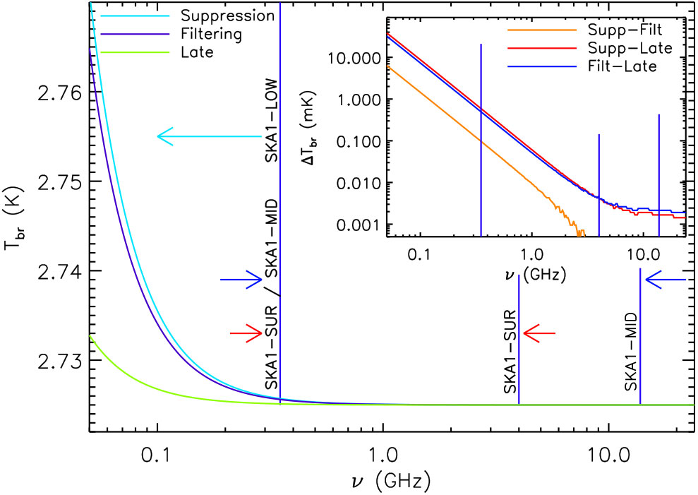
Figure 6. Free-free diffuse signal in the interval of frequencies covered by SKA2 computed for two astrophysical reionisation models (a late phenomenological prescription is also shown). The inset displays the absolute differences between the three models. The vertical lines specify the frequency coverage of SKA1 configurations. Taken from Burigana et al. (Reference Burigana2015). These curves define the minimal FF signal theoretically expected. For extreme models, like those considered by Oh (Reference Oh1999), the FF excess could be even  $\sim\!70$ times larger.
The SKA’s high sensitivity and resolution can provide us relevant information to improve the current knowledge of the CMB spectrum and of the energy exchanges in cosmic plasma. Furthermore, the SKA will help the modelling of galactic emissions and extragalactic (EG) foregrounds, a substantial advancement being necessary to detect and possibly characterise the expected tiny spectral distortions. The EG radio foreground is weaker than the galactic radio emission but, in contrast to the galactic foregrounds that represent the main limitation in CMB spectrum observations, it is difficult to separate it from the cosmological background by analysing its angular distribution properties in the sky because of the limited resolution of experiments devoted to CMB monopole temperature, particularly at low frequencies. The accurate determination of the EG source number counts from the deep SKA surveys allows to compute the source background, improving the quality of its separation in CMB spectrum studies.
SKA will trace the neutral hydrogen distribution and the transition from the essentially neutral to the highly ionised state of the IGM during the dawn age and the reionisation epoch using the 21-cm redshifted line (see e.g., Schneider et al. Reference Schneider, Salvaterra, Choudhury, Ferrara, Burigana and Popa2008). At the same time, it could directly reconstruct the evolution of ionised material by observing the FF emission produced by ionised halos. Reionisation models based on both semi-analytical approaches (Naselsky & Chiang Reference Naselsky and Chiang2004) and numerical computations (Ponente et al. Reference Ponente, Diego, Sheth, Burigana, Knollmann and Ascasibar2011) allow to estimate the expected signal. Dedicated, high-resolution observations may allow one to distinguish the FF spectral distortions by ionised halos from those by diffuse ionised IGM. With SKA2-Low, we could discover up to  $\sim\! 10^{4}$ individual FF emission sources per squared degree at $z>5$, understanding the different contributions from ionised halos and from the diffuse ionised IGM to the global FF cosmological signal (more details are provided by Burigana et al. Reference Burigana2015).
In conclusion, SKA’s precise number counts, particularly at frequencies from  $\sim\! 1$ to a few GHz, will be crucial for a precise analysis of dedicated CMB spectrum measurements. The precise mapping of large and dedicated regions of the sky with the SKA’s extremely good capability of producing interferometric images represents an interesting opportunity to observe diffuse FF emission anisotropies from large to small angular scales and individual halos. Moreover, implementing SKA with very compact configurations and ultra-accurate calibrators could be, in principle, a way to detect the absolute level of diffuse FF emission.
2.4. Detection prospects and challenges with the SKA
Having provided an overview of various fundamental physics constraints which may be achievable with the SKA observations of cosmic dawn and reionisation, we present here a brief summary of the detection prospects, synergies with other probes at these epochs, and the foreground mitigation challenges, which are relevant to recover fundamental physics constraints from these epochs.
2.4.1. Challenges From EoR astrophysics
The astrophysics of the 21-cm line necessarily presents a ‘systematic’ in the study of fundamental physics and cosmology. This is especially true at the EoR and cosmic dawn, in which the various astrophysical processes described in Section 2.2.1 lead to effects which need to be isolated effectively for the measurement of cosmological parameters. Modelling the astrophysics accurately is crucial to be able to distinguish the fundamental physics, and the power spectrum may need to be convolved with astrophysical models (e.g., using codes similar to 21CMFAST Mesinger et al. Reference Mesinger, Furlanetto and Cen2011, described in Section 2.2.1), in order to place competitive constraints on cosmology.
Bayesian inference may be used to interpret the brightness temperature power spectrum in the context of a model and to place constraints on cosmological parameters. In order to do this, analytic or semi-analytic techniques (e.g., Furlanetto et al. Reference Furlanetto, Zaldarriaga and Hernquist2004a; Pritchard & Loeb Reference Pritchard and Loeb2008) are essential, since fast and accurate model parameter evaluation is required. It can be shown that this ‘astrophysical separation’ can be effectively achieved in the post-reionisation Universe using a halo model formalism to describe HI and obtain the uncertainties in the parameters from all the astrophysical constraints (Padmanabhan & Refregier Reference Padmanabhan and Refregier2017; Padmanabhan et al. Reference Padmanabhan, Refregier and Amara2017). The combination of astrophysical constraints at these epochs can be shown to lead to 60%–100% uncertainty levels in the measurement of the HI power spectrum (Padmanabhan et al. Reference Padmanabhan, Choudhury and Refregier2015), which provides a measure of the ‘astrophysical degradation’ relevant for forecasting cosmological and fundamental physics parameters. Similar modelling techniques applied to the high-redshift observations, though expected to be significantly harder, may be used to isolate the astrophysical effects for accurate constraints on the fundamental physics and cosmological parameters as described in the previous sections.
2.4.2. Synergies between 21-cm and galaxy surveys
Cross-correlating different astrophysical probes can eliminate the systematic effects in the measurements, and thus enable tighter constraints on the fundamental physics from the EoR. Several large area surveys of galaxies in the EoR that overlap SKA1 and SKA2 are planned, using, for example, the Hyper-SuprimeCam on Subaru (Lyman- $\alpha$ emitters, LAEs), Euclid (Lyman-break galaxies, LBGs), the Large Synoptic Survey Telescope (LSST, LBGs), and the Wide-Field Infrared Survey Telescope (WFIRST, LAEs, and LBGs).
Galaxy samples from such surveys will provide important calibrations of galaxy population properties during the EoR, such as their clustering strength and star formation rate density. Towards later phases of reionisation, fluctuations in the neutral hydrogen fraction govern the brightness temperature. These fluctuations in turn depend on the properties of the sources, including their clustering (Mellema et al. Reference Mellema2013). Combining data on the population of source galaxies with the global brightness temperature signal measured with SKA at these epochs, the fraction of reionisation that is caused by the galaxies can be constrained (Cohen et al. Reference Cohen, Fialkov, Barkana and Lotem2017). Cross-correlation of the SKA brightness temperatures with the LAE/LBG samples from galaxy surveys provides additional constraints on the reionisation history, for example, to what extent different galaxy populations contribute to reionisation, the evolution of the ionisation fraction, and the topology of reionisation (Hutter et al. Reference Hutter, Dayal, Müller and Trott2017). The brightness temperature can further be correlated with the properties of galaxies directly, for example, from the Euclid or LSST wide+deep surveys (Bacon et al. Reference Bacon2015).
Using targeted observations with near-infrared (NIR)/mid-infrared instruments, for example, the James Webb Space Telescope and the European Extremely Large Telescope, currently uncertain source properties such as the net ionising flux and escape fraction can be constrained spectroscopically (e.g., Jensen et al. Reference Jensen, Zackrisson, Pelckmans, Binggeli, Ausmees and Lundholm2016). The galaxy luminosity function within ionised bubbles identified in the 21-cm brightness temperature maps can also be constrained using these cross-correlations.
In the post-reionisation Universe, cross-correlations can be used to understand the general life cycle of galaxies, which is determined by their star formation activity in relation to the available gas reservoirs. The star formation rate has been observed to peak at redshift 2 (Madau & Dickinson Reference Madau and Dickinson2014) whereas observations of the HI energy density,  $\Omega_{\rm HI}$, with redshift suggest very subtle to non-existing evolution of the gas densities (Prochaska & Wolfe Reference Prochaska and Wolfe2009). This could imply that the molecular phase of hydrogen is the dominant ingredient in galaxy evolution processes (e.g., Lagos et al. Reference Lagos2015; Saintonge et al. Reference Saintonge2016), though it is also tightly connected to the atomic as well as the ionised fractions of the hydrogen.
Mapping the intensity fluctuations of the 21-cm brightness temperature has been attempted in the post-reionisation universe with the Green Bank Telescope (GBT) at  $z\approx 0.8$ (Switzer et al. Reference Switzer2013). Cross-correlating the data with complementary optical galaxy surveys (Masui et al. Reference Masui2013b) increases the detectability of the signal as well as giving a constraint on the average HI contents of the optical objects (Wolz et al. Reference Wolz, Blake and Wyithe2017b).
The SKA provides ample opportunities to extend existing observations to bigger volumes and higher redshifts (Santos et al. Reference Santos2015). In particular, SKA-Low can supply novel information via its proposed IM experiment in the higher frequencies of the aperture array at  $3<z<6$. These observations will be crucial to understand the transitioning process of the cold gas after the EoR as well as the distribution of HI gas in relation to the underlying halo mass and host galaxy properties. Additionally, the cross-correlations of the high-redshift HI datasets with either galaxy surveys or intensity maps of other spectral lines will reveal universal scaling relations of galaxy formation and evolution processes.
2.4.3. Foreground modelling
One of the most significant challenges for an EoR detection is that of the overwhelming foregrounds. The problem is typically broken into three independent components—galactic synchrotron (GS), which contributes around 70% of the total foreground emission (Shaver et al. Reference Shaver, Windhorst, Madau and de Bruyn1999); EG sources (predominantly compact) which contribute about 27% (Mellema et al. Reference Mellema2013); and finally galactic FF emission which constitutes the remaining  $\sim\! 1\%$. Altogether, these foregrounds are expected to dominate the EoR signal brightness by up to five orders of magnitude, though this figure reduces to 2–3 when considering the interferometric observable: angular brightness fluctuations (Bernardi et al. Reference Bernardi2009). Furthermore, each source is expected to predominantly occupy a different region of angular spectral space (Chapman et al. Reference Chapman, Zaroubi, Abdalla, Dulwich, Jeli´c and Mort2016).
All foreground mitigation techniques rely on first subtracting measured components, such as bright compact EG sources in the field-of-view (Pindor et al. Reference Pindor, Wyithe, Mitchell, Ord, Wayth and Greenhill2011), and a diffuse sky model. While significant advances have been made in deep targeted observations of the foregrounds by various instruments (Bernardi et al. Reference Bernardi2009; Bernardi et al. Reference Bernardi2010; Ghosh et al. Reference Ghosh, Bharadwaj, Ali and Chengalur2011; Yatawatta et al. Reference Yatawatta2013; Jelić et al. 2014; Asad et al. Reference Asad2015; Remazeilles et al. Reference Remazeilles, Dickinson, Banday, Bigot-Sazy and Ghosh2015; Offringa et al. Reference Offringa2016; Procopio et al. Reference Procopio2017; Line et al. Reference Line, Webster, Pindor, Mitchell and Trott2017), due to their overwhelming dominance, even the residuals (from faint unmodelled sources and mis-subtraction) necessitate a robust mitigation approach.
The key to signal extraction lies in its statistical differentiation from the foregrounds, and it is well known that such a separation occurs naturally in the frequency (line-of-sight) dimension. While the signal is expected to exhibit structure on scales of  $\sim$ MHz, the foregrounds are predominantly broadband emission, creating a smooth spectral signature. Leveraging this insight, several techniques for foreground residual mitigation have arisen in the past decade. Broadly, they may be split into two categories: (i) foreground subtraction, in which a smooth spectral model is fit and subtracted, and (ii) foreground avoidance, in which Fourier modes, which are known to be foreground-dominated, are eschewed.
2.4.3.1. Foreground subtraction
Foreground subtraction utilises the smoothness of the spectral dependence of the foregrounds in order to fit a smooth model to each angular pixel along the frequency axis. The best-fit model is subtracted, in the hope that the residuals are primarily the EoR signal.
Specific methods in this technique have been further categorised by whether they are ‘blind’: that is, whether they specify a parametric form to be fit, or whether the form is blindly identified by a statistical method.
Parametric methods. The earliest example of foreground modelling was the fitting of smooth polynomials of varying order (e.g., McQuinn et al. Reference McQuinn, Zahn, Zaldarriaga, Hernquist and Furlanetto2006; Bowman et al. Reference Bowman, Morales and Hewitt2006). A more statistical approach is that of ‘correlated component analysis’ (CCA) (Ricciardi et al. Reference Ricciardi2010), which invokes an empirical parametric form for each of the foreground components along with a linear mixing algorithm. For an application of CCA to simulated data, see Bonaldi & Brown (Reference Bonaldi and Brown2015). These methods have the inherent advantage of simplicity and the ability to impose any physical knowledge of the foreground structure directly. Conversely, they suffer from the potential to overfit and destroy the signal, as well as from ambiguity in the specification of a parametrisation.
Non-parametric methods. One may alternatively propose a set of arbitrary bases to assume the role of a mixing matrix in the process of blind source separation. This alleviates the potential for overfitting, and removes the ambiguity of form specification, to the detriment of simplicity and ability to directly input prior knowledge. The most well-known implementations of this approach are fast independent component analysis (Chapman et al. Reference Chapman2012) and generalised morphological component analysis (GMCA; Chapman et al. Reference Chapman2013). The latter appears to be the most robust approach in the foreground subtraction category (Chapman et al. Reference Chapman2015) and has been used as part of the LOFAR EoR pipeline (Patil et al. Reference Patil2017).
2.4.3.2. Foreground avoidance
An inherent danger with foreground subtraction methods is the fact that, even post-subtraction, residuals may dominate over the signal due to overfitting or mis-subtraction. A more conservative route lies in first representing the data as a cylindrical power spectrum, that is, separating line-of-sight modes,  $k_{||}$, from perpendicular modes, $k_\perp$. In this space, the foreground contributions are seen to occupy a low- $k_{||}$ region known as the ‘wedge’. This region has a reasonably sharp demarcation, and its complement is designated the EoR ‘window’ (Liu et al. Reference Liu, Parsons and Trott2014b;a). In principle, a final averaging purely over window modes yields a pristine power spectrum of the signal, and this has been employed by the PAPER project (Ali et al. Reference Ali2015) and can inform instrument design (e.g., DeBoer et al. Reference DeBoer2017).
This approach has the major drawback that a wide range of high-signal modes are unused (Chapman et al. Reference Chapman, Zaroubi, Abdalla, Dulwich, Jeli´c and Mort2016; Liu et al. Reference Liu, Parsons and Trott2014a). A more optimal general approach was developed by Liu et al. (Reference Liu, Parsons and Trott2014b,a), based on the minimum variance estimator formalism of Liu & Tegmark (Reference Liu and Tegmark2011). This method hinges upon defining the data covariance of the ‘junk’ (i.e., the instrumentally distorted foregrounds and other systematics), either empirically (Dillon et al. Reference Dillon2015) or parametrically (Trott et al. Reference Trott2016), and consistently suppresses modes which are foreground-dominated, optimally using all information.
A difficulty with parametric covariance is the suitable specification of the complex foreground models in the presence of instrumental effects. Accordingly, the Cosmological HI Power Spectrum Estimator (Trott et al. Reference Trott2016), for example, employs simplistic prescriptions, with EG sources obeying empirical power-law source counts and uniform spatial distributions, and GS emission obeying an isotropic power-law angular spectrum. Recent studies have begun to relax these simplifications, for example, Murray et al. (Reference Murray, Trott and Jordan2017) define the EG point source covariance in the presence of angular clustering.
2.4.3.3. Summary and outlook
A number of systematic comparisons of foreground mitigation methods have been performed. Chapman et al. (Reference Chapman2015) compared foreground subtraction methods and found that GMCA proves the most robust to realistic foreground spectra. Alonso et al. (Reference Alonso, Bull, Ferreira and Santos2015a) unified a number of subtraction methods under a common mathematical framework and showed that for a large suite of fast simulations the methods perform comparably. Chapman et al. (Reference Chapman, Zaroubi, Abdalla, Dulwich, Jeli´c and Mort2016) compared subtraction with avoidance, finding that they are complementary: avoidance recovers small scales well, while subtraction recovers large scales well. More specifically, Jacobs et al. (Reference Jacobs2016) compared the entire data pipelines used for the MWA analysis, including a basic avoidance technique ( $\epsilon$ppsilon; Barry et al. Reference Barry, Beardsley, Byrne, Hazelton, Morales, Pober and Sullivan2019), empirical covariance (Dillon et al. Reference Dillon2015), and parametric covariance (Trott et al. Reference Trott2016). For the MWA data, each was shown to perform comparably.
Looking to the future, several challenges have been identified. One such challenge is the potential for polarisation leakage, which may induce a higher amplitude of small-scale structure on the foregrounds, obscuring the signal (Moore et al. Reference Moore2017; Asad et al. Reference Asad2015, Reference Asad2016, Reference Asad, Koopmans, Jeli´c, de Bruyn, Pandey and Gehlot2018). Another challenge is to improve the fidelity of EG source covariances. In particular, to date, a distribution of source sizes has not been considered, and neither is the faint source population constrained to any significant degree at EoR-pertinent frequencies. More theoretically, attempts to consistently unify the avoidance and subtraction approaches must be furthered in order to extract maximal information from the data (see e.g., Ghosh et al. Reference Ghosh, Koopmans, Chapman and Jeli´c2015; Sims et al. Reference Sims, Lentati, Alexander and Carilli2016, Reference Sims, Lentati, Pober, Carilli, Hobson, Alexander and Sutter2017 as examples of Bayesian frameworks). Finally, an assortment of instrumental effects such as baseline mode-mixing (Hazelton et al. Reference Hazelton, Morales and Sullivan2013) must be overcome.
Despite these challenges, the increasing depth of low-frequency targeted foreground observations along with theoretical advancement of foreground techniques ensures that the EoR cannot hide forever.
2.5. Summary
We have identified some of the key areas where SKA observations of the 21-cm signal are likely to impact fundamental physics as:
1. Cosmological parameters, especially neutrino mass and constraints on WDM models (and other possible properties of DM).
2. Variations in fundamental constants (e.g., the fine structure constant).
3. Detecting the ISW effect in cross-correlation with galaxy catalogues.
4. Constraints on inflationary models and measurement of the runnings of the spectral index.
5. Tests of statistical anisotropy.
6. CMB spectral distortions and dissipation processes.
We have indicated the challenges in the detection of the EoR signal with upcoming experiments, including the systematic imposed by the uncertainties in the astrophysics during these epochs, and ways to effectively isolate this to recover the underlying fundamental physics. We also briefly described synergies with other surveys during the same epochs, which allow cross-correlations that eliminate systematic effects to a large extent. Finally, we commented on the challenges from foregrounds at these frequencies, and the techniques for the foreground mitigation by both subtraction and avoidance methods.
Overall, the combination of (i) accurate astrophysical modelling of reionisation and the first stars, (ii) advances in detection techniques and foreground mitigation, and (iii) synergies with various other cosmological probes promises an optimistic outlook for observing the epochs of cosmic dawn and reionisation with the SKA, and for deriving exciting fundamental physics constraints from these as yet unobserved phases of the Universe.
3. Gravity and gravitational radiation
Gravity plays a crucial role in astrophysics on all scales. While Einstein’s General Theory of Relativity is our best theory, meeting all observational tests to date, there remain a number of open problems in astrophysics and cosmology that have, at their heart, the question of whether GR is the correct theory of gravity. In this section, we consider the ways in which the SKA will bring new opportunities for tests of theories of gravity at various length scales.
3.1. Introduction
3.1.1. GR and modified gravity
To date, GR has passed every test with flying colours. The most stringent of these have been carried out in the solar system and with binary pulsars (Will Reference Will2014; Stairs Reference Stairs2003; Wex Reference Wex2014; Shao & Wex 2016; Kramer Reference Kramer2016), where a wide range of deviations from GR have been essentially ruled out with extremely high precision. The recent direct measurement of GWs by Advanced LIGO/Virgo has produced a new opportunity to validate GR in a very different physical situation, that is, a highly dynamical, strong field spacetime (Abbott et al. 2016c; Reference Abbott2017), and a growing variety of cosmological tests of gravity are beginning to be carried out with ever-increasing precision (Joyce et al. Reference Joyce, Jain, Khoury and Trodden2015; Bull et al. Reference Bull2016). These are just a few of the regimes in which new gravitational phenomena could be hiding, however (Baker et al. Reference Baker, Psaltis and Skordis2015), and most have not yet been tested with the high precision that is characteristic of solar system tests. Furthermore, intriguing clues of possible deviations from GR have been emerging (e.g., in recent studies of DM and dark energy) but are far from decisive and remain open to interpretation. Finally, GR may turn out to be the low-energy limit of a more fundamental quantum gravity theory, with hints of the true high-energy theory only arising in relatively extreme physical situations that we have yet to probe. As such, testing GR across a broader range of physical regimes, with increasing precision, stands out as one of the most important tasks in contemporary fundamental physics. The SKA will be a remarkably versatile instrument for such tests, as we will discuss throughout this section.
An important tool in extending tests of GR into new regimes has been the development of a variety of alternative gravity theories (Clifton et al. Reference Clifton, Ferreira, Padilla and Skordis2012b). These give some ideas of what possible deviations from GR could look like and help to structure and combine observational tests in a coherent way. While there are many so-called modified gravity theories in existence, it is possible to categorise them in a relatively simple way, according to how they break Lovelock’s theorem (Lovelock Reference Lovelock1971). This is a uniqueness theorem for GR; according to Lovelock’s theorem, GR is the only theory that is derived from a local, four-dimensional action that is at most second order in derivatives only of the spacetime metric. Any deviation from these conditions breaks the theorem, giving rise to an alternative non-GR theory that may or may not have a coherent structure. For example, one can add additional gravitational interactions that depend on new scalar or tensor degrees of freedom (e.g., Horndeski or bigravity models respectively), add extra dimensions (e.g., Randall-Sundrum models), introduce non-local operators (e.g., non-local gravity), higher-order derivative operators (e.g., f(R) theory), or even depart from an action-based formulation altogether (e.g., emergent spacetimes). Each of these theories tends to have a complex structure of its own, which is often necessary to avoid pathologies such as ghost degrees of freedom, derivative instabilities, and so forth. Viable theories are also saddled with the need to reduce to a theory very close to GR in the solar system, due to the extremely restrictive constraints on possible deviations in that regime. The result is that most viable modified gravity theories predict interesting new phenomena—for example, screening mechanisms that shield non-GR interactions on small scales as in Chameleon gravity (Khoury & Weltman Reference Khoury and Weltman2004a,b)—which in turn inform the development of new observational tests. Unsuccessful searches for these new phenomena can constrain and even rule out specific subsets of these theories and test GR in the process.
3.1.1.1. Testing relativistic gravity with radio pulsar timing
Pulsar timing involves the use of large area radio telescopes or arrays to record the so-called times of arrival (TOAs) of pulsations from rotating radio pulsars. Millisecond pulsars (MSPs) are especially stable celestial clocks that allow timing precision at the nanosecond level (Taylor Reference Taylor1992; Stairs Reference Stairs2003). Such precision enables unprecedented studies of neutron star astronomy and fundamental physics, notably precision tests of gravity theories (Wex Reference Wex2014; Manchester:Reference Manchester2015; Kramer Reference Kramer2016).
The TOAs from pulsar timing depend on the physical parameters that describe the pulsar system. These include the astrometric and rotational parameters of the pulsar, velocity dispersion in the intervening interstellar medium, and the motion of the telescope in the solar system (including the movement and the rotation of the Earth). If the pulsar is in a binary system, the TOAs are also affected by the orbital motion of the binary, which in turn depend on the underlying gravity theory (Damour & Taylor Reference Damour and Taylor1992; Edwards et al. Reference Edwards, Hobbs and Manchester2006). Deviations from GR—if any—will manifest in TOAs, and different kinds of deviations predict different residuals from the GR template.
The double pulsar J0737–3039 (Kramer et al. Reference Kramer2006) represents the state-of-the-art in the field. Five independent tests have already been made possible with this system. GR passes all of them. When the SKA is operating, the double pulsar will provide completely new tests, for example, measuring the Lense–Thirring effect (Kehl et al. Reference Kehl, Wex, Kramer and Liu2017), which probe a different aspect of gravitation related to the spin.
What makes the field of testing gravity with pulsar timing interesting is that, although the double pulsar represents the state-of-the-art, other pulsars can outperform it in probing different aspects of gravity (Wex Reference Wex2014). For example, the recently discovered triple pulsar system (with one neutron star and two white dwarfs) is the best system to constrain the universality of free fall (UFF) for strongly self-gravitating bodies (Ransom et al. Reference Ransom2014; Shao Reference Shao2016; Archibald et al. Reference Archibald2018). UFF is one of the most important ingredients of the strong equivalence principle (SEP; Will Reference Will2014). When UFF is violated, objects with different self-gravitating energies could follow different geodesics (Damour & Schaefer Reference Damour and Schaefer1991). When the SEP is violated, for a binary composed of two objects with different self-gravitating energies, it is very likely that a new channel to radiate away orbital energy will open. If dipole radiation exists (in addition to the quadrupole radiation in GR), a binary will shrink faster, resulting in a new contribution to the time derivative of the orbital period (Damour & Taylor Reference Damour and Taylor1992). For example, this happens in a class of scalar-tensor theories (Damour & Esposito-Farese Reference Damour and Esposito-Farese1996), and in these theories, the dipole radiation might also be enhanced due to the strong field of neutron star interiors. Binary pulsars have provided the best constraints for this phenomenon (Freire et al. Reference Freire2012; Shao et al. Reference Shao, Sennett, Buonanno, Kramer and Wex2017).
Pulsars can be used to test the validity of theories (de Cesare & Sakellariadou Reference de Cesare and Sakellariadou2017; de Cesare et al. Reference de Cesare, Lizzi and Sakellariadou2016) that lead to time variation of Newton’s gravitational constant. A time-varying Newton’s constant will contribute to the decay of the binary orbit as (Damour et al. Reference Damour, Gibbons and Taylor1988; Nordtvedt Reference Nordtvedt1990)
 $$
\begin{equation}
{\dot P\over P}=-2{\dot G\over G}\left[ 1-\left( 1+{m_c\over 2M} \right) s
\right] ~,
\label{eqn3}
\end{equation}
$$
$$
\begin{equation}
{\dot P\over P}=-2{\dot G\over G}\left[ 1-\left( 1+{m_c\over 2M} \right) s
\right] ~,
\label{eqn3}
\end{equation}
$$ where P,  $m_c$, and M stand for the orbital period, the companion mass, and the sum of the masses of the pulsar and its companion, respectively, and s denotes a sensitivity parameter. Currently, the strongest constraint on the temporal variation of the gravitational constant results from lunar laser ranging analysis, which sets (Williams et al. Reference Williams, Turyshev and Boggs2004)
 $$
\begin{equation}
{\dot G\over G}=(4\pm 9)\times 10^{-13} \, {\rm yr}^{-1}~.
\label{eqn4}
\end{equation}
$$
$$
\begin{equation}
{\dot G\over G}=(4\pm 9)\times 10^{-13} \, {\rm yr}^{-1}~.
\label{eqn4}
\end{equation}
$$Pulsar timing of PSRs J1012+5307 (Lazaridis et al. Reference Lazaridis2009), J1738+0333 (Freire et al. Reference Freire2012), and J1713+0747 (Zhu et al. Reference Zhu2019) has achieved limits comparable to Equation (4).
Binary pulsars can also be used to test cosmological models that lead to local Lorentz invariance (LLI) violation. In particular, some modified gravity models, such as the TeVeS (Bekenstein Reference Bekenstein2004) or the D-material universe (a cosmological model motivated from string theory that includes a vector field; Elghozi et al. Reference Elghozi, Mavromatos, Sakellariadou and Yusaf2016) imply violation of LLI. Possible violation of LLI results in modifications of the orbital motion of binary pulsars (Damour & Esposito-Farese Reference Damour and Esposito-Farese1992; Shao & Wex Reference Shao and Wex2012; Shao Reference Shao2014), as well as leads to characteristic changes in the spin evolution of solitary pulsars (Nordtvedt Reference Nordtvedt1987; Shao et al. Reference Shao, Caballero, Kramer, Wex, Champion and Jessner2013); for the latter, LLI also leads to spin precession with respect to a fixed direction (Shao & Wex Reference Shao and Wex2012). Hence, LLI violation implies changes in the time derivative of the orbit eccentricity, of the projected semi-major axis, and of the longitude of the periastron, while it changes the time behaviour of the pulse profile. The strongest current constraints on LLI violation are set from pulsar experiments, using the timing of binary pulsars.
There is also the potential for the SKA to search for the predicted effects of quantum gravity. Specifically, in a pulsar BH binary system, the disruption effect due to quantum correction can lead to a different gravitational time delay and interferometry of BH lensing. Recently, the discovery of PSR J1745–2900 (Eatough et al. Reference Eatough2013; Rea et al. Reference Rea2013; Shannon & Johnston Reference Shannon and Johnston2013) orbiting the galactic centre (GC) BH Sgr A* opens up the possibility for precision tests of gravity (Pen & Broderick Reference Pen and Broderick2014). The radio pulses emitted from the pulsar can be lensed by an intervening BH that is in between the pulsar and observer. Therefore, the gravitational time delay effect and interferometry between the two light rays can be used to investigate the possible quantum deviations from standard Einstein gravity (Pen & Broderick Reference Pen and Broderick2014). According to Pen & Broderick (Reference Pen and Broderick2014), the fractal structure of the BH surface due to quantum corrections can destroy any interference between the two light rays from the pulsars. In the future, the SKA will find a large number of pulsar BH binary systems, with which we will be able to perform stringent tests of gravity.
Finally, binary pulsars have been used to constrain a free parameter of a higher-derivative cosmological model, obtained as the gravitational sector of a microscopic model that offers a purely geometric interpretation for the standard model (Chamseddine et al. Reference Chamseddine, Connes and Marcolli2007). By studying the propagation of gravitons (Nelson et al. Reference Nelson, Ochoa and Sakellariadou2010b), constraints were placed on the parameter that relates coupling constants at unification, using either the quadrupole formula for GWs emitted from binary pulsars (Nelson et al. Reference Nelson, Ochoa and Sakellariadou2010a) or geodesic precession and frame-dragging effects (Lambiase et al. Reference Lambiase, Sakellariadou and Stabile2013). These constraints will be improved once more rapidly rotating pulsars close to the Earth are observed. Clearly, such an approach can be used for several other extended gravity models (Capozziello et al. Reference Capozziello, Lambiase, Sakellariadou and Stabile2015; Lambiase et al. Reference Lambiase, Sakellariadou, Stabile and Stabile2015).
Since the SKA will provide better timing precision and discover more pulsars, all the above tests will be improved significantly (Shao et al. Reference Shao2015).
3.1.1.2. BH physics and Sgr A*
Testing BH physics is an intriguing and challenging task for modern astronomy. Relativity predicts that any astrophysical BH is described by the Kerr metric and depends solely on its mass and angular momentum (or equivalently spin). Sagittarius A* (Sgr A*), which is the closest example of a supermassive BH (SMBH), is an ideal laboratory with which the SKA can test gravity theories and the no-hair theorem (Kramer et al. Reference Kramer, Backer, Cordes, Lazio, Stappers and Johnston2004).
Pulsars are extremely precise natural clocks due to their tremendous rotational stability. Thus, a relativistic binary of a pulsar and Sgr A* would be a robust tool for testing relativity in stronger gravitational fields than is available from pulsar binaries with stellar mass companions. Such a test will be important since strong field predictions can be fundamentally different between GR and a number of alternative gravity theories (see Johannsen Reference Johannsen2016, for a review).
The GC hosts a large number of young and massive stars within the inner parsec, which can be the progenitors of pulsars (e.g., Paumard et al. Reference Paumard2006; Lu et al. Reference Lu, Do, Ghez, Morris, Yelda and Matthews2013). The population of normal pulsars can be hundreds within distance of  $<\!4000AU$ from Sgr A* (e.g., Zhang et al. Reference Zhang, Lu and Yu2014; Pfahl & Loeb Reference Pfahl and Loeb2004; Chennamangalam & Lorimer Reference Chennamangalam and Lorimer2014). The orbits of the innermost ones could be as tight as $\sim\!100$–500 AU from the SMBH (Zhang et al. Reference Zhang, Lu and Yu2014). Furthermore, a magnetar recently discovered in this region (Rea et al. Reference Rea2013; Eatough et al. Reference Eatough2013) also suggests that a population of normal pulsars is likely to be present near the GC, since magnetars are rare pulsars.
To reveal pulsars in the GC region, a high-frequency (usually  $>\!9$ GHz) radio survey is needed as there is severe radio scattering by the interstellar medium at low frequencies. Radio surveys so far have not found any normal pulsars in the innermost parsec of the GC (e.g., Deneva et al. Reference Deneva, Cordes and Lazio2009; Macquart et al. Reference Macquart, Kanekar, Frail and Ransom2010; Bates et al. Reference Bates2011). SKA1-Mid would be capable of revealing pulsars down to $2.4$ GHz with spin periods $\sim\! 0.5$ s in this region (Eatough et al. Reference Eatough2015). The timing accuracy of pulsars for SKA after $\sim1$ h integration can reach $\sigma_T\simeq100\,\mu$s (Liu et al. Reference Liu, Wex, Kramer, Cordes and Lazio2012) at a frequency of $\gtrsim15\,$GHz, and $\sigma_T\simeq0.1$– $10\,$ms if the frequency is between $\gtrsim\! 5\,$ and $\lesssim\! 15\,$GHz. Besides the timing measurements, proper motions would be measurable for these pulsars. Finally, the baselines of the SKA are expected to be up to $\sim 3000\,$km, and thus it can provide image resolution up to $2\,$mas at $10\,$GHz (Godfrey et al. Reference Godfrey2012) and astrometric precision reaching $\sim\!10\,\mu$ as (Fomalont & Reid Reference Fomalont and Reid2004).
The relativistic effects cause orbital precession of the pulsars orbiting Sgr A*, in both the argument of pericentre and the orbital plane. A number of previous studies have focused on the relativistic effects according to the orbital averaged precession over multiple orbits (e.g., Wex & Kopeikin Reference Wex and Kopeikin1999; Pfahl & Loeb Reference Pfahl and Loeb2004; Liu et al. Reference Liu, Wex, Kramer, Cordes and Lazio2012; Psaltis et al. Reference Psaltis, Wex and Kramer2016) or the resolved orbital precession within a few orbits (Angélil & Saha Reference Angélil and Saha2010; Angélil et al. Reference Angélil, Saha and Merritt2010). These studies implement post-Newtonian techniques based on Blandford & Teukolsky (Reference Blandford and Teukolsky1976), Damour & Deruelle (Reference Damour and Deruelle1986), and Hobbs et al. (Reference Hobbs, Edwards and Manchester2006), or a mixed perturbative and numerical approach (Angélil et al. Reference Angélil, Saha and Merritt2010). For a pulsar orbiting an SMBH, it is also feasible to implement full relativistic treatments (Zhang et al. Reference Zhang, Lu and Yu2015; Zhang & Saha Reference Zhang and Saha2017).
The TOAs of pulsars rotating around Sgr A* are affected by a number of relativistic effects, for example, Einstein delay and Shapiro delay (Damour & Deruelle Reference Damour and Deruelle1986; Taylor Reference Taylor1992). The orbital precession caused by frame-dragging and quadrupole moment effects also impact the TOAs. Recent studies have found that the frame-dragging effect in TOAs for a pulsar-Sgr A* binary are quite strong compared to the timing accuracies of the pulsar (Liu et al. Reference Liu, Wex, Kramer, Cordes and Lazio2012; Psaltis et al. Reference Psaltis, Wex and Kramer2016), that is, orders of 10–100 s per orbit while the timing accuracies are typically  $\sim0.1$ ms (Zhang & Saha Reference Zhang and Saha2017). Current TOA modelling assumes that the orbital precession increases linearly with time. However, it is found to be inaccurate compared to the TOA accuracy; thus, more sophisticated modelling of TOAs are needed, for example, explicitly solving the geodesic equation of the pulsars and the propagation trajectories of the photons (Zhang & Saha Reference Zhang and Saha2017).
Frame-dragging and quadrupole momentum effects can be tightly constrained by observing relativistic pulsar-Sgr A* binaries. If the orbital period of a pulsar is  $\sim\!0.3$ yr, the frame-dragging and the quadrupole moment effect of the SMBH can be constrained down to $\sim10^{-2}$– $10^{-3}$ and $\sim10^{-2}$, respectively, within a decade, providing timing accuracies of
  $\sigma_{\rm
T}\sim100\,\mu$s (Liu et al. Reference Liu, Wex, Kramer, Cordes and Lazio2012). By monitoring a normal pulsar with an orbital period of
$\sigma_{\rm
T}\sim100\,\mu$s (Liu et al. Reference Liu, Wex, Kramer, Cordes and Lazio2012). By monitoring a normal pulsar with an orbital period of  $\sim2.6$ yr and an eccentricity of $0.3$– $0.9$, and assuming a timing accuracy of 1–5 ms, the magnitude, the line-of-sight inclination, the position angle of the SMBH spin can be constrained with $2\sigma$ errors of $10^{-3}$– $10^{-2}$, $0.1^\circ$– $5^\circ$, and $0.1^\circ$– $10^\circ$, respectively, after $\sim$8 yr (Zhang & Saha Reference Zhang and Saha2017). Even for pulsars in orbits similar to the currently detected stars S2/S0-2 or S0-102, the spin of the SMBH can still be constrained within 4– $8\,$yr (Zhang & Saha Reference Zhang and Saha2017); see Figure 7. Thus, any pulsar located closer than $\sim\! 1000$ AU from the SMBH is plausible for GR spin measurements and tests of relativity.
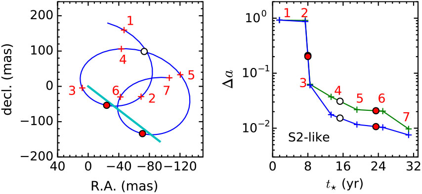
Figure 7. Left: Apparent trajectories on the sky: blue for the pulsar and cyan for the SMBH. Right: Accuracy on the recovered spin magnitude, with green showing results when TOAs on their own are used, and blue showing results from combining both timing and proper motion information. (Zhang & Saha Reference Zhang and Saha2017). The filled red and empty white circles mark the pericentre and apocentre, respectively, of the pulsar orbit. The curves are interpolated from the computed accuracies at the epochs labelled 1–7.
Combining timing and astrometric measurements of GC pulsars, the mass and distance of Sgr A* can be constrained with extremely high accuracy. If the proper motion of pulsars can be determined with an accuracy of  $10\,\mu$ as along with timing measurements, the mass and the distance of the SMBH can be constrained to about $\sim 1\,{\rm M}_\odot$ and $\sim1\,$pc, respectively (Zhang & Saha Reference Zhang and Saha2017).
It is important to note, however, that GC pulsars would experience gravitational perturbations from other masses, such as stars or other stellar remnants. These (non-relativistic) perturbations may obscure the spin-induced signals outside  $\gtrsim\!100$– $400\,\rm ~AU$ (Merritt et al. Reference Merritt, Alexander, Mikkola and Will2010; Zhang & Iorio Reference Zhang and Iorio2017). Outside this region, how to remove this Newtonian ‘foreground’ remains an unsolved problem. One possible filtering strategy may be to use wavelets (Angélil & Saha Reference Angélil and Saha2014).
3.1.1.3. Cosmological tests of gravity
While GR has proven robust against all observational and experimental tests that have been carried out so far, most of these have been restricted to the solar system or binary pulsar systems—that is, firmly in the small-scale, weak field regime. The recent LIGO GW detection has added a valuable strong field test of GR to the roster, but it is the relatively poorly constrained cosmological regime that has perhaps the greatest chance of offering a serious challenge to Einstein’s theory. The application of GR to cosmology represents an extrapolation by many orders of magnitude from where the theory has been most stringently tested, out to distance scales where unexpected new gravitational phenomena—specifically, DM and dark energy—have been discovered to dominate the Universe’s evolution. While it may yet be found that these have ‘conventional’ explanations, perhaps in terms of extensions to the standard model of particle physics, the fact remains that they have so far only been detected through their gravitational influence. As such, it is of utmost importance to examine whether the extrapolation of GR out to cosmological distances could be to blame for the appearance of these effects—perhaps we are interpreting our observations in the context of the wrong gravitational theory.
Cosmological tests of GR are still in their infancy, however. While most ‘background’ cosmological parameters are now known to better than 1% precision, additional parameters that describe possible deviations from GR are considerably less well constrained. Recent measurements of the growth rate of LSS have been made at the 10% level, for example, while many alternative theories of gravity have never even been subjected to tests beyond a comparison with background parameter constraints from, e.g., the CMB. It is clear, then, that there is some way to go before constraints on GR in the cosmological regime approach the accuracy that has been achieved in the small-scale, weak field limit.
The SKA is expected to play a central role in a multitude of high-precision tests of GR in cosmological settings, often in synergy with other survey experiments in different wavebands. In this section, we consider several examples of how SKA1 and SKA2 will contribute to precision cosmological tests of GR, including: growth rate and slip relation measurements with galaxy clustering and weak lensing observations; tests of gravity and dark energy using the 21-cm IM technique; detecting relativistic effects on ultra-large scales; peculiar velocity surveys; and void statistics.
On linear sub-horizon scales, there are two main ways in which deviations from GR can affect cosmological observables: by modifying how light propagates, and by modifying how structures collapse under gravity (Amendola et al. Reference Amendola, Kunz, Motta, Saltas and Sawicki2013). Both effects can be probed using large statistical samples of galaxies, for example, by measuring the weak lensing shear and RSD signals. At optical wavelengths, these observations are the preserve of photometric (imaging) and spectroscopic redshift surveys, respectively, but radio observations offer several alternative possibilities for getting at this information.
3.1.1.4. Radio weak lensing
Effective weak lensing surveys can be performed using radio continuum observations (Brown et al. Reference Brown2015), where the total emission from each galaxy is integrated over the entire waveband to increase signal-to-noise. SKA1-Mid has excellent  $u-v$ plane coverage, making it possible to image large numbers of galaxies and measure their shapes. It will perform a large continuum galaxy survey over an area of several thousand square degrees (Jarvis et al. Reference Jarvis, Bacon, Blake, Brown, Lindsay, Raccanelli, Santos and Schwarz2015a), achieving a sky density of suitable lensed sources of 2.7 arcmin–2 at a mean redshift of $\sim\! 1.1$ (Harrison et al. Reference Harrison, Camera, Zuntz and Brown2016). This is a substantially lower number density than contemporary optical surveys, for example, the Dark Energy Survey (DES) will yield $\sim\! 12$ arcmin–2 at a mean redshift of 0.6. However, forecasts suggest that the two surveys should constrain cosmological parameters with a similar level of accuracy—for example, both SKA1 and DES lensing surveys should produce $\mathcal{O}(10\%)$ constraints on the parameter $\Sigma_0$, which parametrises deviations of the lensing potential from its GR behaviour (Harrison et al. Reference Harrison, Camera, Zuntz and Brown2016). This is mainly due to the stronger lensing signal from a significant high-redshift tail of continuum sources that compensate for the lower source number density. Corresponding forecasts for SKA2 suggest that a number density of 10 arcmin–2 will be achievable at a mean redshift of 1.3, for a survey covering 30 000 deg $^2$, yielding $\sim\! 4\%$ constraints on $\Sigma_0$ (Harrison et al. Reference Harrison, Camera, Zuntz and Brown2016), surpassing what will be possible with Euclid. While SKA alone will produce strong constraints on modified gravity lensing parameters, the combination of SKA with optical lensing surveys should be the ultimate goal, as the two different methods have very different systematics that should mostly drop out in cross-correlation, producing much ‘cleaner’ lensing signals with enhanced signal-to-noise (Bonaldi et al. Reference Bonaldi, Harrison, Camera and Brown2016; Camera et al. Reference Camera, Harrison, Bonaldi and Brown2017).
3.1.1.5. RSD and peculiar velocities from HI galaxies
SKA1 will have the sensitivity and spectral resolution to perform several different types of spectroscopic galaxy surveys, using the 21-cm emission line from HI. The simplest is a redshift survey, where the 21-cm line is detected for as many galaxies as possible, with a signal-to-noise ratio sufficient only to get a fix on each redshift. Both SKA1 and SKA2 will be able to perform very large redshift surveys; the SKA1 version will be restricted to quite low redshifts, due to the steepness of the sensitivity curve for HI (Yahya et al. Reference Yahya, Bull, Santos, Silva, Maartens, Okouma and Bassett2015; Harrison et al. Reference Harrison, Lochner and Brown2017), while the SKA2 version will be essentially cosmic variance limited from redshift 0 to  $\sim\! 1.4$ for a survey covering 30 000 deg $^2$ (Yahya et al. Reference Yahya, Bull, Santos, Silva, Maartens, Okouma and Bassett2015; Bull Reference Bull2016). Precise spectroscopic redshifts allow the galaxy distribution to be reconstructed in 3D down to very small scales, where density fluctuations become non-linear, and galaxies have substantial peculiar velocities due to their infall into larger structures. These velocities distort the 3D clustering pattern of the galaxies into an anisotropic pattern, as seen in redshift-space. The shape of the anisotropy can then be used to infer the velocity distribution, and thus the rate of growth of LSS. HI redshift surveys with SKA1 and SKA2 will both be capable of precision measurements of these RSDs, with SKA1 yielding $\sim\! 10\%$ measurements of $f\sigma_8$ (the linear growth rate multiplied by the normalisation of the matter power spectrum) in several redshift bins out to $z \approx 0.5$, and SKA2 yielding $\lesssim\! 1\%$ measurements out to $z \approx 1.7$ (Bull Reference Bull2016). See Figure 8 for a comparison with other surveys.
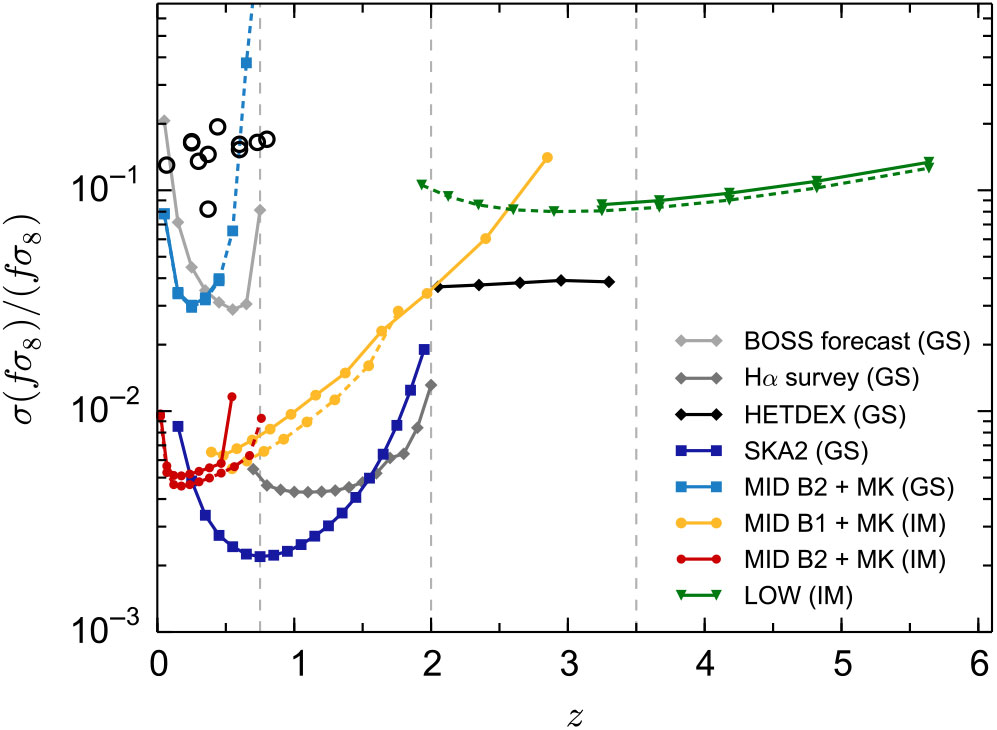
Figure 8. Comparison of predicted constraints on the growth rate,  $f\sigma_8$, from RSD measurements with various SKA and contemporary optical/NIR surveys. ‘GS’ denotes a spectroscopic galaxy survey, while ‘IM’ denotes an IM survey. The open circles show a compilation of recent RSD measurements. Taken from Bull (Reference Bull2016).
Note that redshift surveys are not the only possibility—one can also try to spectrally resolve the 21-cm lines of galaxies with high signal-to-noise ratios, and then measure the width of the line profile to obtain their rotation velocities. This can then be used in conjunction with the Tully–Fisher (TF) relation that connects rotation velocity to intrinsic luminosity to directly measure the distances to the galaxies, making it possible to separate the cosmological redshift from the Doppler shift due to the peculiar velocity of the galaxy. Direct measurements of the peculiar velocity are highly complementary to RSDs, as they measure the growth rate in combination with a different set of cosmological parameters (i.e., they are sensitive to  $\alpha = f[z] H[z]$). The recovered velocity field can also be cross-correlated with the density field (traced by the galaxy positions), resulting in a significant enhancement in the achievable growth rate constraints if the source number density is high enough (Koda et al. Reference Koda2014). SKA1 will be able to perform a wide, highly over-sampled TF peculiar velocity measurement at low redshift (cf., the sensitivity curves of Yahya et al. Reference Yahya, Bull, Santos, Silva, Maartens, Okouma and Bassett2015), potentially resulting in better constraints on the growth rate than achievable with RSDs. The peculiar velocity data would also be suitable for testing (environment-dependent) signatures of modified gravity due to screening, as discussed by Hellwing et al. (Reference Hellwing, Barreira, Frenk, Li and Cole2014) and Ivarsen et al. (Reference Ivarsen, Bull, Llinares and Mota2016).
3.1.1.6. 21-cm IM
Twenty-one centimetre IM (Battye et al. Reference Battye, Davies and Weller2004; Chang et al. Reference Chang, Pen, Peterson and McDonald2008) is an innovative technique that uses HI to map the three-dimensional LSS of the Universe. Instead of detecting individual galaxies like traditional optical or radio galaxy surveys, HI IM surveys measure the intensity of the redshifted 21-cm emission line in three dimensions (across the sky and along redshift).
The possibility of testing dark energy and gravity with the SKA using 21-cm IM has been studied extensively (Santos et al. Reference Santos2015). More specifically, it has been shown that an IM survey with SKA1-Mid can measure cosmological quantities like the Hubble rate H(z), the angular diameter distance  $D_{\rm A}(z)$, and the growth rate of structure $f\sigma_8(z)$ across a wide range of redshifts (Bull et al. Reference Bull, Ferreira, Patel and Santos2015), at a level competitive with the expected results from Stage IV optical galaxy surveys like Euclid (Amendola et al. Reference Amendola2018). For example, a very large area SKA1-Mid IM survey can achieve sub-1% measurements of $f\sigma_8$ at $z<1$ (Bull Reference Bull2016).
However, the IM method is still in its infancy, with the major issue being foreground contamination (which is orders of magnitude larger than the cosmological signal) and systematic effects. These problems become much more tractable in cross-correlation with optical galaxy surveys, since systematics and noise that are relevant for one type of survey but not the other are expected to drop out (Masui et al. Reference Masui2013a; Pourtsidou et al. Reference Pourtsidou, Bacon, Crittenden and Metcalf2016; Wolz et al. Reference Wolz2017a). Therefore, cross-correlating the 21-cm data with optical galaxies is expected to alleviate various systematics and lead to more robust cosmological measurements.
As an example, we can consider cross-correlating an HI IM survey with SKA1-Mid with a Euclid-like optical galaxy clustering survey, as discussed by Pourtsidou et al. (Reference Pourtsidou, Bacon and Crittenden2017). Assuming an overlap  $A_{\rm sky} = 7000 \, {\rm deg}^2$, it was found that very good constraints can be achieved in ( $f\sigma_8, D_{\rm A}, H$) across a wide redshift range $0.7 \leq z \leq 1.4$, where dark energy or modified gravity effects are important (see Table 1). Furthermore, it was found that combining such a survey with CMB temperature maps can achieve an ISW detection with a signal-to-noise ratio $\sim\! 5$, which is similar to the results expected from future Stage IV galaxy surveys. Detecting the ISW effect in a flat universe provides direct evidence for dark energy or modified gravity.
Table 1. Forecasted fractional uncertainties on  $\{f\sigma_8, D_{\rm A}, H\}$ assuming the SKA1-Mid IM and Euclid-like spectroscopic surveys.
3.1.1.7. Relativistic effects on ultra-large scales
Thanks to the unmatched depth of continuum radio galaxy surveys, the large sky coverage, and the novel possibilities available with HI IM, the SKA will probe huge volumes of the Universe, thus allowing us to access the largest cosmic scales. Scales close to the cosmic horizon and beyond carry valuable information on both the primeval phases of the Universe’s evolution and on the law of gravity.
On the one hand, peculiar inflationary features such as primordial non-gaussian imprints are the strongest on the ultra-large scales. On the other hand, if we study cosmological perturbations with a fully relativistic approach, a plethora of terms appears in the power spectrum of number counts besides those due to Newtonian density fluctuations and RSDs (Challinor & Lewis Reference Challinor and Lewis2011; Bonvin & Durrer Reference Bonvin and Durrer2011; Yoo et al. Reference Yoo, Hamaus, Seljak and Zaldarriaga2012; Jeong et al. Reference Jeong, Schmidt and Hirata2012; Alonso et al. Reference Alonso, Bull, Ferreira, Maartens and Santos2015b). For instance, lensing is known to affect number counts through the so-called magnification bias; but other, yet-undetected effects like time delay, gravitational redshift and Sachs-Wolfe and ISW-like terms also contribute to the largest cosmic scales. To measure such relativistic corrections would mean to further thoroughly confirm Einstein’s gravity, in a regime far from where we have accurate tests of it. Otherwise, if we found departures from the well known and robust relativistic predictions, this would strongly hint at possible solutions of the DM/energy problems in terms of a modified gravity scenario (Lombriser et al. Reference Lombriser, Yoo and Koyama2013; Baker et al. Reference Baker, Ferreira, Leonard and Motta2014b; Baker & Bull Reference Baker and Bull2015).
Alas, measurements on horizon scales are plagued by cosmic variance. For instance, forecasts for next-generation surveys show that relativistic effects will not be detectable using a single tracer (Camera et al. Reference Camera2015e; Alonso & Ferreira Reference Alonso and Ferreira2015) and primordial non-gaussianity detection is limited to  $\sigma(\,f_{\rm NL})\gtrsim 1$ (Camera et al. Reference Camera, Santos and Maartens2015a; Raccanelli et al. Reference Raccanelli2015). This calls for the multi-tracer technique (MT), developed for biased tracer of the large-scale cosmic structure and able to mitigate the effect of cosmic variance (Seljak Reference Seljak2009; Abramo & Leonard Reference Abramo and Leonard2013; Ferramacho et al. Reference Ferramacho, Santos, Jarvis and Camera2014). Fonseca et al. (Reference Fonseca, Camera, Santos and Maartens2015) showed that the combination of two contemporaneous surveys, a large HI IM survey with SKA1 and a Euclid-like optical/NIR photometric galaxy survey, will provide detection of relativistic effects, with a signal-to-noise of about 14. Forecasts for the detection of relativistic effects for other combinations of radio/optical surveys are discussed by Alonso & Ferreira (Reference Alonso and Ferreira2015).
3.1.1.8. Void statistics
As a particular case for the SKA, we consider number counts of voids, and forecast cosmological parameter constraints from future SKA surveys in combination with Euclid, using the Fisher matrix method (see also 5.4.2). Considering that additional cosmological information is also available in, for example, shapes/profiles, accessible with the SKA, voids are a very promising new cosmological probe.
We consider a flat wCDM cosmology (i.e., a CDM cosmology with a constant equation of state, w) with a modified gravity model described by a growth index  $\gamma(a) = \gamma_0 + \gamma_1(1-a)$ (Di Porto et al. Reference Di Porto, Amendola and Branchini2012). The void distribution is modelled following Sahlén et al. (Reference Sahlén, Zubeldia and Silk2016) and Sahlén & Silk (Reference Sahlén and Silk2018), here also taking into account the galaxy density and bias for each survey (Yahya et al. Reference Yahya, Bull, Santos, Silva, Maartens, Okouma and Bassett2015; Raccanelli et al. Reference Raccanelli, Montanari, Bertacca, Doré and Durrer2016c). The results are shown in Figure 9. The combined SKA1-Mid and Euclid void number counts could achieve a precision $\sigma(\gamma_0) = 0.16$ and $\sigma(\gamma_1) = 0.19$, marginalised over all other parameters. The SKA2 void number counts could improve on this, down to $\sigma(\gamma_0) = 0.07$, $\sigma(\gamma_1) = 0.15$. Using the powerful degeneracy-breaking complementarity between clusters of galaxies and voids (Sahlén et al. Reference Sahlén, Zubeldia and Silk2016; Sahlén & Silk Reference Sahlén and Silk2018; Sahlén Reference Sahlén2019), SKA2 voids + Euclid clusters number counts could reach $\sigma(\gamma_0) = 0.01$, $\sigma(\gamma_1) = 0.07$.
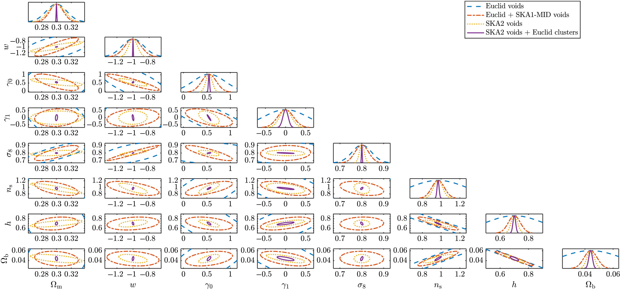
Figure 9. Forecast 68% parameter confidence constraints for a flat wCDM model with time-dependent growth index of matter perturbations. Note the considerable degeneracy breaking between the Euclid and SKA1 void samples, and between the SKA2 void and Euclid cluster samples. SKA1-Mid covers 5 000 deg $^2$,
$^2$,  $z = 0-0.43$. SKA2 covers 30 000 deg $^2$,
$^2$,  $z=0.1-2$. Euclid voids covers 15 000 deg $^2$,
$^2$,  $z=0.7-2$. Euclid clusters covers 15 000 deg $^2$,
$^2$,  $z=0.2-2$. The fiducial cosmological model is given by $\{\Omega_{\rm m} = 0.3, w = -1, \gamma_0 = 0.545, \gamma_1 = 0, \sigma_8 = 0.8, n_{\rm s} = 0.96, h = 0.7, \Omega_{\rm b} = 0.044\}$. We have also marginalised over uncertainty in void radius and cluster mass (Sahlén & Silk Reference Sahlén and Silk2018), and in the theoretical void distribution function (Pisani et al. Reference Pisani, Sutter, Hamaus, Alizadeh, Biswas, Wandelt and Hirata2015).
3.2. GW astronomy
3.2.1. Understanding GW sources
GWs may be sourced by an astrophysical object (compact objects such as neutron stars and BHs) or they can be of a cosmological origin. Binaries of coalescing compact objects constitute the main goal of ground-based interferometers. Processes operating in the early Universe may lead to a stochastic GW background, offering a unique opportunity to understand the laws that operated at such high energies, as GWs are out of thermal equilibrium since the Planck scale. Possible sources of GWs of cosmological origin are inflation, particle production, preheating, topological defects like cosmic strings, and first-order phase transitions.
3.2.2. Detection of GWs with SKA galaxy surveys
Galaxy catalogues can be used to detect GWs; the idea of looking at the angular motion of sources both in the Milky Way (Jaffe Reference Jaffe2004; Book & Flanagan Reference Book and Flanagan2011) and on EG scales dates back to the 1980s (see, for example, Linder Reference Linder1986, Linder Reference Linder1988; Braginsky et al. Reference Braginsky, Kardashev, Polnarev and Novikov1990; Kaiser & Jaffe Reference Kaiser and Jaffe1997).
The possibility of detecting GWs using SKA galaxy surveys has been investigated recently by Raccanelli (Reference Raccanelli2017), by looking at what has been defined ‘cosmometry’, that is, the high-redshift equivalent of astrometry: the passage of a stochastic gravitational wave background (SGWB) will cause the angular position of distant sources to oscillate. The oscillations have a zero average, but the RMS is proportional to the strain of the passing GWs. Therefore, by means of a statistical analysis of galaxy correlations, it could be possible to detect GWs from the early Universe.
Another possibility comes from using galaxy catalogues obtained with the SKA and their statistics to detect the presence of an SGWB from the effect of tensor perturbations; GWs are tensor perturbations, and so a background of them will have effects on galaxy clustering and gravitational lensing statistics (see also Jeong & Schmidt Reference Jeong and Schmidt2012; Schmidt & Jeong Reference Schmidt and Jeong2012).
3.2.3. Pulsar timing arrays
Pulsar timing arrays (PTAs) use the ‘quadrupole correlation’ (the Hellings–Downs curve) in the timing residuals from an array of pulsars, aiming to detect low-frequency GWs in the frequency range  $10^{-9}-10^{-6}$ Hz (Hellings & Downs Reference Hellings and Downs1983; Foster & Backer Reference Foster and Backer1990; Hobbs & Dai Reference Hobbs and Dai2017). The Parkes PTA collaboration (PPTA; Manchester et al. Reference Manchester2013) was established in 2004, followed in 2007 by the European PTA (EPTA; Kramer & Champion Reference Kramer and Champion2013), and the North American Nanohertz Observatory for Gravitational Waves (NANOGrav; McLaughlin Reference McLaughlin2013). PPTA, EPTA, and NANOGrav form the International PTA collaboration (IPTA; Verbiest et al. Reference Verbiest2016) to share data and algorithms among different PTAs. When the SKA is online, it will boost the PTA efforts to detect low-frequency GWs (Kramer et al. Reference Kramer, Backer, Cordes, Lazio, Stappers and Johnston2004; Janssen et al. Reference Janssen2015).
There are various GW sources for PTAs (Janssen et al. Reference Janssen2015). For example, cosmic strings, one-dimensional topological defects, arise naturally in many field theories as a particular class of false vacuum remnants (Jeannerot et al. Reference Jeannerot, Rocher and Sakellariadou2003). A loop of invariant string length  $\ell$ has a period $T=\ell/2$ and oscillates at a fundamental frequency $\omega=4\pi/\ell$. Hence, it radiates GWs with frequencies that are multiples of $\omega$ and decays in a lifetime $\ell/(100 G\mu)$, where G is Newton’s constant and $\mu$ is the mass per unit length for cosmic strings. The loop contribution to the stochastic GW background is expressed in terms of the frequency f as,
 $$
\begin{equation}
\Omega_{\rm GW}={f\over \rho_{\rm c}} {d\rho_{\rm GW}\over df}~,
\label{eqn5}
\end{equation}
$$
$$
\begin{equation}
\Omega_{\rm GW}={f\over \rho_{\rm c}} {d\rho_{\rm GW}\over df}~,
\label{eqn5}
\end{equation}
$$ where  $\rho_{\rm c}$ denotes the critical energy density of the Universe, and $\rho_{\rm GW}$ depends on the string linear density and, therefore, on the temperature of the phase transition followed by spontaneous symmetry breaking leading to the cosmic string production. Pulsar timing experiments are able to test the spectrum of GWs at nanohertz frequencies, while LIGO/Virgo detectors are sensitive in the 10–1000 Hz band.
For understanding the impact of SKA on pulsar timing-based GW detection, it is important to estimate the total number of MSPs that can be discovered with the SKA and the typical root mean square (RMS) noise level of pulsar TOAs that can be attained.
In one survey scenario (Smits et al. Reference Smits2011), SKA1-Mid is expected to detect 1200 MSPs in 53 d of telescope time, and this number will climb up to 6000 MSPs with SKA2-Mid (Smits et al. Reference Smits, Kramer, Stappers, Lorimer, Cordes and Faulkner2009). It is predicted that one timing observation for 250 MSPs at a signal-to-noise ratio of  $\sim\! 100$ each—the level at which GW detection becomes feasible for anticipated sources—can be obtained with 6–20 h of telescope time on SKA2-Mid.
The timing precision is determined by the noise budget of the measured TOAs. The RMS of the pulse phase jitter noise and the radiometer noise, the most important noise sources at 100 ns timing precision level, can be estimated by (Cordes & Shannon Reference Cordes and Shannon2010; Wang Reference Wang2015)
 $$
\begin{equation}
\sigma_{\rm j} \approx 0.28 W\sqrt{\frac{P}{t}} \;,
\label{eqn6}
\end{equation}
$$
$$
\begin{equation}
\sigma_{\rm j} \approx 0.28 W\sqrt{\frac{P}{t}} \;,
\label{eqn6}
\end{equation}
$$ $$
\begin{equation}
\sigma_{\rm r} \approx \frac{W S}{F\sqrt{2\Delta f t}}\sqrt{\frac{W}{P-W}} \;.
\label{eqn7}
\end{equation}
$$
$$
\begin{equation}
\sigma_{\rm r} \approx \frac{W S}{F\sqrt{2\Delta f t}}\sqrt{\frac{W}{P-W}} \;.
\label{eqn7}
\end{equation}
$$ Here P is the pulsar period, t is the integration time, W is the effective pulse width, F is the flux density,  $\Delta f$ is the bandwidth, and $S=\frac{2\eta k}{A_{\rm e}}T_{\rm sys}$ is the system equivalent flux density (Wilson et al. Reference Wilson, Rohlfs and Hüttemeister2013), where $\eta$ is the system efficiency factor ( $\sim 1.0$), $T_{\rm sys}$ is the system temperature, $A_{\rm e}$ is the effective collecting area, and k is Boltzmann’s constant. Using the design parameters for SKA2 and the relevant physical parameters for individual pulsars obtained from simulations (Smits et al. Reference Smits, Kramer, Stappers, Lorimer, Cordes and Faulkner2009), one finds that for SKA2 the pulse phase jitter noise will be the dominant noise source, comparable to the radiometer noise for most of MSPs. The RMS of total noise $\sigma_t$ for measured TOA is the quadratic summation of jitter noise and radiometer noise, that is, $\sigma_{t}^{2} = \sigma_{j}^{2} + \sigma_{r}^{2}$.
Figure 10 shows the number of MSPs that can achieve 50, 100, 200, and 500 ns timing precisions, respectively, with varying integration time, t. It turns out that if we choose  $t=5$ min for SKA2-Mid, then there can be about 900 MSPs (out of 6000 MSPs considered by Smits et al. Reference Smits, Kramer, Stappers, Lorimer, Cordes and Faulkner2009) timed to an RMS level of 100 ns or better. One caveat of our calculation is that we have not considered red timing noise, which is usually less than 100 ns for MSPs (Shannon & Cordes Reference Shannon and Cordes2010). Assessing the timing noise in terms of amplitude and spectral index of individual MSPs is one of the most crucial tasks in the data analysis for detecting GWs with PTAs (e.g., Arzoumanian et al. Reference Arzoumanian2016).
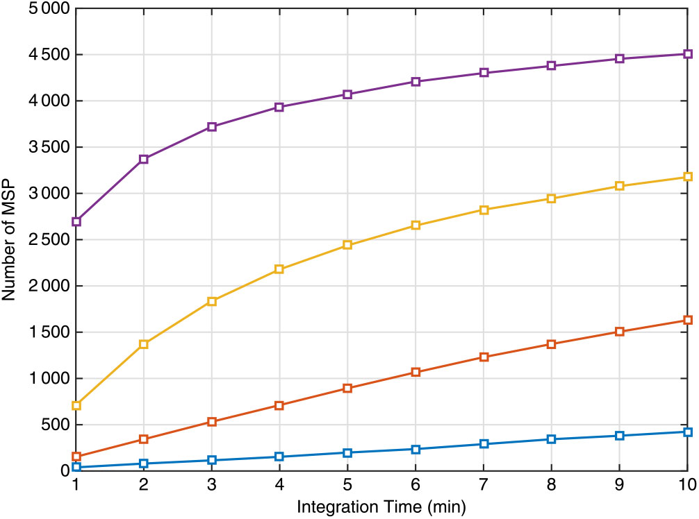
Figure 10. Numbers of MSPs that can archive a certain RMS noise level (or better) with varying integration time. Colour lines indicate different RMS noise levels (from bottom to top): 50 ns (blue), 100 ns (red), 200 ns (yellow), and 500 ns (purple).
Based on these estimates, it appears that a SKA-era PTA with  $\sim\! 1000$ MSPs timed to $\lesssim\! 100$ ns at a cadence of one timing observation every 2 weeks may be feasible. Such a PTA will reach a sensitivity that will allow, for example, a $10^{10}$ ${\rm M}_\odot$ redshifted chirp mass supermassive black hole binary (SMBHB) to be detected out to $z\simeq 28$ and a $10^{9}$ ${\rm M}_\odot$ redshifted chirp mass SMBHB to be detected out to $z\simeq 1-2$. This will enable high confidence detection of GWs from some of the existing optically identified SMBHB candidates (Wang & Mohanty Reference Wang and Mohanty2017).
Besides the stochastic GW signal from the unresolved SMBHB population that may be detected with SKA1 itself (Janssen et al. Reference Janssen2015), it is likely that some individual SMBHBs will stand out above the SGWB and become resolvable. The data analysis challenge of resolving multiple sources from a background population is likely to be a significant one given the large number of SMBHBs that will be uncovered by an SKA-era PTA. The PTA data analysis methods for resolvable sources (e.g., Ellis et al. Reference Ellis, Siemens and Creighton2012; Zhu et al. Reference Zhu2015; Wang et al. Reference Wang, Mohanty and Jenet2014, Reference Wang, Mohanty and Jenet2015, Reference Wang, Mohanty and Qian2017) must be able to handle multiple sources while taking into account (i) the SGWB from unresolved sources that acts as an unmodelled noise source and (ii) instrumental and timing noise characterisation across  $\sim\! 10^3$ MSPs. Previous studies (e.g., Babak & Sesana Reference Babak and Sesana2012; Petiteau et al. Reference Petiteau, Babak, Sesana and de Araújo2013) of multiple source detection have assumed a simplified model of the GW signal in which the so-called pulsar term is dropped and the signal is embedded in white noise with no SGWB. Further development of data analysis methods that can work without these simplifying assumptions is required.
3.3. Primordial GWs (B-modes): Polarised foregrounds with SKA
The angular power spectrum of polarised anisotropies in the CMB can be decomposed into E-modes, mainly generated by perturbations of scalar type in the primordial Universe, and B-modes that could be mainly contributed at low multipoles,  $\ell$, (i.e., large angular scales) by primordial tensor metric perturbations.Footnote g Detecting and characterising primordial B-modes likely represent the unique way to firmly investigate the stochastic field of primordial GWs through the analysis of tensor perturbations they produce. Although other mechanisms can produce tensor perturbations, the multipole dependence of primordial B-modes generated by cosmic inflation is relatively well predicted while their overall amplitude, related to the ratio, $r = T/S$, of tensor to scalar primordial perturbations depends on the inflation energy scale. For this reason, the detection of primordial B-modes received special attention in current and future CMB polarisation experiments (see, e.g., André et al. Reference André2014; Ishino et al. Reference Ishino2016; Finelli et al. Reference Finelli2018, and references therein).
The foreground signal from EG radio sources (see, e.g., De Zotti et al. Reference De Zotti2018, and references therein) generates the most relevant source of contamination for CMB analyses in total intensity and in polarisation at subdegree angular scales up to a frequency of  $\sim\! 100$ GHz. The precise modelling of radio source contribution to polarisation anisotropies at small scales is crucial for the accurate treatment and subtraction of the B-mode signal generated by the lensing effect produced on CMB photons by cosmic structures, intervening between the last scattering surface and the current time. Improving lensing subtraction implies a better understanding of the primordial B-modes at intermediate and low multipoles. Thus, the precise assessment of radio source foreground is fundamental for CMB angular power spectrum analyses, and especially for the discovery of primordial B-modes, particularly in the case of low values of r, and, in general, to accurately characterise them. This step needs precise measurements of the contribution of radio sources down to several factors below the source detection threshold of the CMB experiment, related to the noise, background, and foreground amplitudes depending on the considered sky area. Indeed, for microwave surveys with $\sim$ arcmin resolution and sensitivity from tens to few hundreds of mJy, sources below the detection limit largely contribute to polarisation fluctuations. However, modern radio interferometers with sensitivity and resolution much better than those of CMB experiments can reveal these source populations. At the same time, complementary high-sensitivity polarisation observations at the frequencies where CMB experiments are carried out will provide useful data for both generating adequate masks and statistically characterising source populations to subtract their statistical contribution below the detection thresholds in angular power spectrum analyses. The SKA will allow researchers to perform deep observations of polarised sources only up to $\sim\! 20$ GHz, but probing the extremely faint tail of their flux density distribution. The estimation of the source polarisation fluctuations from SKA data requires one to extrapolate them to higher frequencies where CMB anisotropies are better determined, and the related errors decrease with the decreasing of flux density detection limits. Thus, the combination of ultra-deep SKA surveys with millimetric observations will be very fruitful to characterise source contribution to polarisation fluctuations at small scales, and then to improve lensing and delensing treatment from high to low multipoles.
An accurate description of SKA continuum surveys can be found in Prandoni & Seymour (Reference Prandoni and Seymour2015). The very faint tail of source counts can be firmly assessed by deep and ultra-deep surveys. Furthermore, it is possible to extend the analysis to even weaker flux densities, below the sensitivities of the considered surveys, using methods as described by Condon et al. (Reference Condon2012). This is particularly promising at low frequencies in the case of the continuum surveys dedicated to non-thermal emission in clusters and filaments. The ultra-deep SKA survey aimed at studying the star formation history of the Universe is planned to have a RMS sensitivity of some tens of nJy per beam with a resolution at arcsec level or better,Footnote h to be compared, for example, with the sensitivity levels of tens of  $\mu$Jy of present determination of radio source counts at GHz frequencies (see e.g., Prandoni et al. Reference Prandoni, Gregorini, Parma, de Ruiter, Vettolani, Wieringa and Ekers2001; Condon et al. Reference Condon2012), thus representing a substantial improvement for the measurement of number counts and fluctuations of very faint sources. Figure 11 compares the CMB primordial B-mode angular power spectrum for different values of r with the lensing signal and potential residual foregrounds. The signal of the B-mode angular power spectrum for radio sources is displayed for various detection limits, adopting the radio source fluctuation conservative model of Tucci & Toffolatti (Reference Tucci and Toffolatti2012). Even considering errors from frequency extrapolation (as generously accounted in the Figure assuming a very prudential threshold for the signal), this analysis shows that SKA characterisation of radio source polarisation properties will allow one to reduce their potential residual impact on polarisation fluctuations at essentially negligible levels.
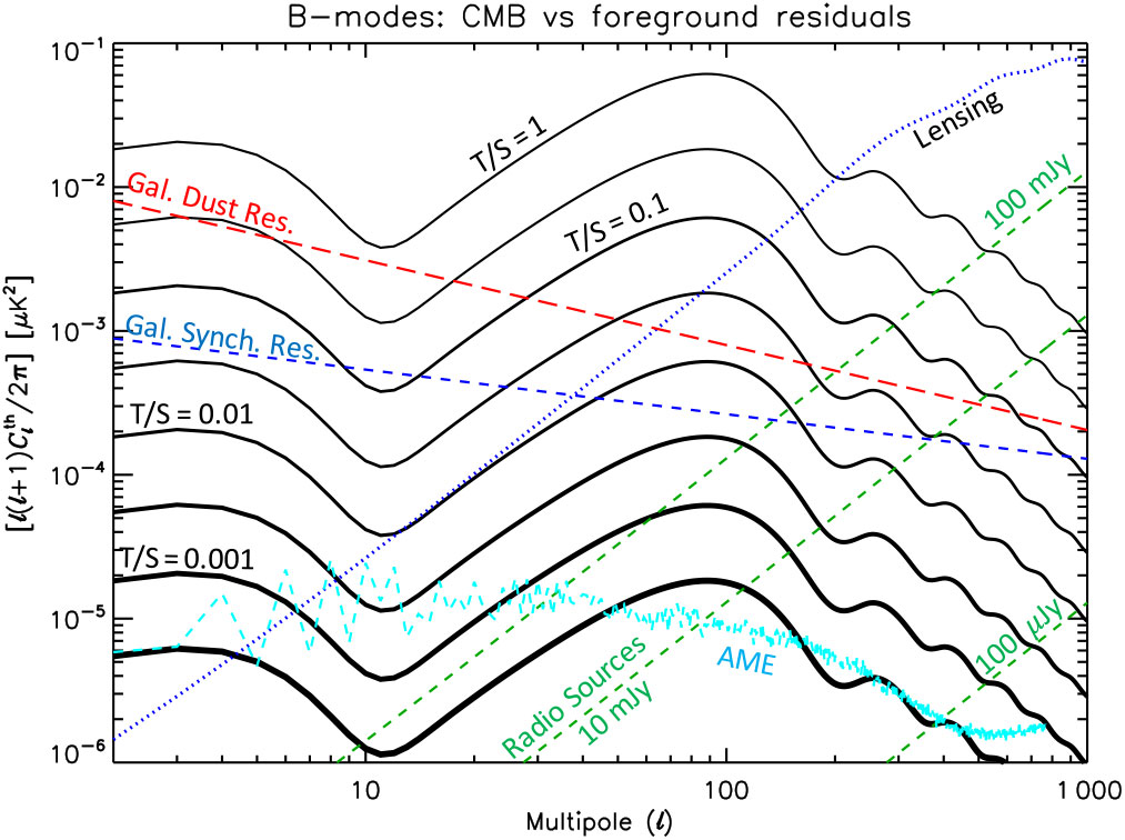
Figure 11. The CMB primordial B-mode polarisation angular power spectrum for different tensor-to-scalar perturbation ratios (from 1 to  $3 \times 10^{-4}$; solid black lines) and, separately, the lensing contribution (blue dots). They are compared with estimates of potential residuals from galactic foregrounds (at 70 GHz) and angular power spectrum from polarised radio sources (at 100 GHz) below different detection thresholds (green dashes; from top to bottom, 100 and 10 mJy, representative of thresholds achievable, respectively, in current and future CMB experiments, and 100 $\mu$Jy representative of potential improvement discussed here). Red long dashes show typical potential residuals from galactic polarised dust emission extrapolated from 353 GHz assuming an error of 0.01 in the dust grain spectral index. Blue dashes show typical potential residuals from galactic polarised synchrotron emission extrapolated from 30 GHz assuming an error of 0.02 in the synchrotron emission spectral index. Azure dashes show an estimate of galactic AME angular power spectrum scaled from total intensity to polarisation assuming a polarisation degree of 2% with, conservatively, all the power in the B-mode (a power two times smaller is expected assuming equal power in E- and B-modes).
Moreover, with the SKA it will be possible to improve our understanding of galactic diffuse foregrounds at low frequencies, where polarised synchrotron emission peaks, a key point for B-mode searches, considering that CMB experiments are typically carried out at higher frequencies. This will have particular implications for (i) GS emission models, (ii) the tridimensional treatment of the Galaxy, as well as (iii) the component of its magnetic field coherent on large scale (Sun et al. Reference Sun, Reich, Waelkens and Enßlin2008; Sun & Reich 2009; Reference Sun and Reich2010; Fauvet et al. 2011; Reference Fauvet, Macías-Pérez and Désert2012) that rely on modern numerical methods (Strong & Moskalenko Reference Strong and Moskalenko1998; Waelkens et al. Reference Waelkens, Jaffe, Reinecke, Kitaura and Enßlin2009) and turbulence (Cho & Lazarian Reference Cho and Lazarian2002). For cosmological applications, it may be critical to better characterise also the anomalous microwave emission (AME) that is found to be correlated with dust emission in the far-infrared and is generated by rapidly spinning small dust grains having an electric dipole moment. While its spectrum likely peaks at  $\sim\!15$–50 GHz, its polarisation degree on very wide sky areas, likely at the percent level, is still almost unknown. SKA2 will allow to derive accurate maps of AME at low frequencies.
In Figure 11, the CMB B-mode angular power spectrum is compared with potential contaminations from galactic emissions (evaluated in a sky region excluding the  $\sim\! 27$% sky fraction mostly affected by galactic emission) estimated on the basis of Planck 2015 results (Planck Collaboration et al. Reference Collaboration2016b,g). As is well known, the polarised emission from galactic dust mostly impacts CMB B-mode analyses (BICEP2/Keck Collaboration et al. 2015; Planck Collaboration et al. Reference Collaboration2016a), but for detecting and characterising B-modes for $r \lesssim$ some $\times 10^{-2}$, the accurate understanding of all types of polarised foreground emissions, including synchrotron and AME, is also crucial.
Many cosmological studies are based on analyses carried out on very wide sky areas, thus calling for accurate, large sky coverage galactic radio emission mapping. The SKA1 continuum surveys (Prandoni & Seymour Reference Prandoni and Seymour2015) at 1.4 GHz and at 120 MHz, to be performed integrating for about 1–2 yr, will have a  $\sim$ 75% sky coverage. A comparison in terms of sensitivity per resolution element with the radio surveys currently exploited in CMB projects data analysis (La Porta et al. Reference La Porta, Burigana, Reich and Reich2008) allows one to appreciate the significant improvement represented by future SKA surveys. The SKA 1.4-GHz survey has, in fact, a sensitivity target $\sim\! 20$ times better than the best currently available all-sky 1.4 GHz radio surveys, while the SKA 120-MHz survey is planned to improve in sensitivity of about a factor of 4 with respect to the 408 MHz Haslam map (Haslam et al. Reference Haslam, Salter, Stoffel and Wilson1982).
3.3.1. Galaxy-GW cross-correlation
SKA galaxy maps can be cross-correlated with GW maps from, for example, laser interferometers to obtain novel measurements potentially able to probe gravity in new ways. One such possibility involves the correlation of GW maps with galaxy catalogues in order to determine the nature of the progenitors of binary BHs. This can be also used to obtain ultra-high precision estimation of cosmological parameters (see e.g., Cutler & Holz Reference Cutler and Holz2009), to test cosmological models (Camera & Nishizawa Reference Camera and Nishizawa2013), or to set constraints on the relation between distance and redshift (Oguri Reference Oguri2016).
Using the same approach, Raccanelli et al. (Reference Raccanelli, Kovetz, Bird, Cholis and Munoz2016b) suggested that the cross-correlation between star-forming galaxies and GW maps could constrain the cosmological model in which PBHs are the DM (see Section 5.3.6.4 for a discussion of this possibility). Here we follow the same approach, focusing on stellar mass PBHs, in the mass window probed by the LIGO instrument.
Using galaxy number counts, one can observe the correlation between galaxies and the hosts of binary BH mergers. We can compute what constraints on the abundance of PBHs as DM (for the same model of Bird et al. Reference Bird, Cholis, Muñoz, Ali-Haïmoud, Kamionkowski, Kovetz, Raccanelli and Riess2016) can be set by cross-correlating SKA surveys with LIGO and Einstein Telescope (ET) GW maps. Considering angular power spectra  $C_\ell$, that can be computed as (see e.g., Raccanelli et al. Reference Raccanelli, Bonaldi, Negrello, Matarrese, Tormen and de Zotti2008; Pullen et al. Reference Pullen, Chang, Doré and Lidz2013):
 $$
\begin{align}
C_{\ell}^{XY}(z,z') &= \left< a^X_{\ell m}(z) a^{Y\,^*}_{\ell m}(z') \right> \nonumber\\[4pt]
&= r \int \frac{4\pi dk}{k} \Delta^2(k) W_{\ell}^X(k, z) W_{\ell}^Y(k, z') \, ,
\label{eqn8}\end{align}
$$
$$
\begin{align}
C_{\ell}^{XY}(z,z') &= \left< a^X_{\ell m}(z) a^{Y\,^*}_{\ell m}(z') \right> \nonumber\\[4pt]
&= r \int \frac{4\pi dk}{k} \Delta^2(k) W_{\ell}^X(k, z) W_{\ell}^Y(k, z') \, ,
\label{eqn8}\end{align}
$$ with  $W_{\ell}^{[X,Y]}$ the window functions of the distribution of sources of different observables, $\Delta^2(k)$ the dimensionless matter power spectrum, and r the coefficient of cross-correlation.
We consider radio survey maps from the S-cubed simulationFootnote i, using the SEX and SAX catalogues, for continuum and HI, respectively, applying a cut to the simulated data appropriate for the assumed flux limit for the considered cases. For all surveys, we take  $f_{\rm sky} =0.75$.
The distribution of GW events can be estimated by:
 $$
\begin{equation}
\frac{d N_{GW}(z)}{dz} \approx \mathcal{R}^m(z) \tau_{\rm obs} \frac{4\pi\chi^2(z)}{(1+z)H(z)} \, ,
\label{eqn9}
\end{equation}
$$
$$
\begin{equation}
\frac{d N_{GW}(z)}{dz} \approx \mathcal{R}^m(z) \tau_{\rm obs} \frac{4\pi\chi^2(z)}{(1+z)H(z)} \, ,
\label{eqn9}
\end{equation}
$$ where  $\mathcal{R}^m(z)$ is the merger rate, $\tau_{\rm obs}$ the observation time, and H(z) the Hubble parameter.
An important factor to understand the nature of the progenitors of binary BH mergers is given by the halo bias of the hosts of the mergers. We assume that mergers of objects at the endpoint of stellar evolution would be in galaxies hosting large numbers of stars, hence being in halos of  $\sim 10^{11-12} {\rm M}_\odot$, the great majority of mergers of primordial binaries will happen within haloes of $< 10^{6} {\rm M}_\odot$, as demonstrated by Bird et al. (Reference Bird, Cholis, Muñoz, Ali-Haïmoud, Kamionkowski, Kovetz, Raccanelli and Riess2016). The discrimination can happen then because these two types of haloes are connected to different amplitudes of the galaxy bias. Specifically, we take galaxies hosting stellar GW binaries to have properties related to SFG galaxy samples. Therefore, we can use $b^{\rm Stellar}_{GW} = b_{\rm SFG}$, assuming its redshift-dependent values as in Ferramacho et al. (Reference Ferramacho, Santos, Jarvis and Camera2014). Conversely, small haloes hosting the majority of PBH mergers are expected to have $b\lesssim 0.6$, approximately constant in our redshift range (Mo & White Reference Mo and White1996). Thus, assuming SFGs bias as $b(z) > 1.4$, we take, as the threshold for a model discrimination, $\Delta_b = b_{\rm SFG} - b_{\rm GW} \gtrsim 1$; given that this threshold should, in fact, be larger at higher redshifts, our assumption can be seen as conservative.
Taking the specifications of planned future surveys, we forecast the measurement uncertainties with the Fisher matrix formalism (Tegmark et al. Reference Tegmark, Hamilton, Strauss, Vogeley and Szalay1998):
 $$
\begin{equation}
F_{\alpha\beta} = \sum_{\ell} \frac{\partial C_\ell}{\partial
\vartheta_\alpha}
\frac{\partial C_\ell}{\partial
\vartheta_\beta} {\sigma_{C_\ell}^{-2}} \, ,
\label{eqn10}
\end{equation}
$$
$$
\begin{equation}
F_{\alpha\beta} = \sum_{\ell} \frac{\partial C_\ell}{\partial
\vartheta_\alpha}
\frac{\partial C_\ell}{\partial
\vartheta_\beta} {\sigma_{C_\ell}^{-2}} \, ,
\label{eqn10}
\end{equation}
$$ with  $\vartheta_{\alpha, \beta}$ being the parameters to be measured, and the power spectra derivatives are computed at fiducial values $\bar \vartheta_{\alpha}$ and the measurement errors are $\sigma_{C_\ell}$.
We compute the amplitude of the cross-correlation marginalising over the galaxy bias factor, assuming a prior of 1% precision on galaxy bias from external measurements.
We imagine multiple GW detector configurations, observing the whole sky; naturally, the precision of the localisation of GW events has a fundamental role in determining the constraining power on the cross-correlation galaxies-GW, as does the maximum redshift observable. We choose the following specifications for GW interferometers:
• aLIGO:  $\ell_{\rm max} = 20$, $z_{\rm max} = 0.75$;
• LIGO-net:  $\ell_{\rm max} = 50$, $z_{\rm max} = 1.0$;
• Einstein Telescope:  $\ell_{\rm max} = 100$, $z_{\rm max} = 1.5$;
where with LIGO-net we assume a network of interferometers including the current LIGO detectors, VIRGO, and the planned Indian IndIGO and the Japanese KAGRA instruments, in order to achieve a few square degrees of angular resolution. For assigning statistical redshifts to radio continuum catalogues, we follow the technique of Kovetz et al. (Reference Kovetz, Raccanelli and Rahman2017).
In Figure 12, we plot the forecasts (at 1- $\sigma$ level) for three different GW interferometer configurations, after 5 yr of data collection, assuming a merger rate $\mathcal{R}=10$ Gpc $^3$ yr–1, correlated with SKA radio surveys. The correlation of HI and continuum surveys will not be different if correlating with LIGO and a future LIGO-NET. On the other hand, in the ET case, there will be an effect due to the maximum redshift probed.

Figure 12. Forecast fraction of DM in PBH, for different fiducial experiment sets. For details on GW experiments, see text.
As one can see, aLIGO will be able to derive only weak constraints on the effects of PBHs as DM when correlating GWs with a survey detecting a few thousand sources per deg $^2$ (or observing for a longer time). However, future correlations of LIGO-net or the ET with radio surveys in continuum with some redshift information can deliver a clear detection for $f_{\rm PBH}=1$, or the hints of PBHs that comprise a small part of the DM. Other current and future constraints on PBHs as DM are discussed in Section 5.3.6.4.
3.3.1.1. Pulsar timing array
Multiple resolvable systems may be detectable in the pulsar timing data due to the fact that an SKA-era PTA can detect SMBHBs residing at high redshifts. Correlating the GW signal with optical variability in follow-up observations can teach us much about the physical process in accreting SMBHBs. The distance reach of the SKA-era PTA also implies that high-redshift SMBHB candidates pinpointed in time domain optical observations, such as PG 1302–102 (Graham et al. Reference Graham2015), can be followed up in the GW window. The direct detection of the GW signal from an optically identified candidate SMBHB will confirm its true nature.
Accretion onto an SMBHB may produce periodic variability in the light curve of a quasar (Macfadyen & Milosavljevic Reference Macfadyen and Milosavljevic2008; Graham et al. Reference Graham2015; Hayasaki & Loeb Reference Hayasaki and Loeb2016). Since the study of quasar optical variability is a key scientific goal for LSST (LSST Science Collaboration et al. 2009), numerous SMBHB candidates may be discovered during the survey lifetime. The LSST cadence per object will yield  $\sim\! 1$ measurement of flux per week, which implies that source variability frequency up to $10^{-6}$ Hz can be detected. This yields a good overlap with SMBHB orbital frequencies in the $[5\times 10^{-10}, 10^{-6}]$ Hz interval that are observable with PTAs. Similarly, the LSST coverage of active galactic nuclei (AGN) will reach a redshift of $~7.5$, overlapping the SKA era PTA distance reach for SMBHBs.
LSST full science operation is scheduled to begin around 2023, which coincides with the start date of SKA1. Thus, LSST and SKA1 will have a substantial overlap in observation of sources over a common period of time. There will also be some overlap with SKA2 when it starts around 2030. In the absence of a significant overlap, SKA2-era PTA-based GW searches can be correlated against optically identified candidates in archival LSST data. LSST observations can help narrow down the parameter space to be searched in the PTA data analysis. This is especially important if the source is strongly evolving. The sky location of the source can tell us which MSPs to time with higher precision and faster cadence.
There will be significant data analysis challenges involved in linking PTA-based GW searches in the SKA era with LSST. The sky localisation accuracy of a PTA-based search for SMBHBs depends on the source brightness and sky location. Given the typical localisation error on the sky of approximately  $100~{\rm deg}^2$ (Wang & Mohanty Reference Wang and Mohanty2017) for bright sources, a source detected by a SKA-era PTA is likely to be associated with a large number of variable objects. However, the frequency of optical variability and that of the GW signal, the latter being quite accurately measurable, are likely to be strongly related and this can help in significantly narrowing down the set of candidates to follow-up.
3.4. Summary
Gravity and gravitational radiation are central topics in modern astrophysics. The SKA will have a major impact in this field, via:
1. Better timing of binary pulsar systems, in order to probe new aspects of the gravitational interaction, for example, measurement of the Lense–Thirring effect;
2. Discovery of pulsar binaries orbiting stellar mass BHs or Sgr A*, which will enable novel tests such as the no-hair theorem and even some quantum gravity scenarios;
3. Galaxy clustering, weak lensing, 21-cm IM, peculiar velocity surveys, and void statistics, with which we can study gravitational interactions at cosmological scales with great precision;
4. Cross-correlation of radio weak lensing surveys and HI IM with optical lensing surveys and optical galaxy clustering surveys, respectively, in order to reduce associated systematics and achieve better sensitivities;
5. Synergies with other GW observations (e.g., the B-modes in the primordial GWs), using SKA galaxy surveys and polarisation foreground observations;
6. Direct detection of GWs at nanohertz frequencies with pulsar timing arrays.
Studies of gravitation with the SKA will not be limited to the above items. Various possible synergies with other large surveys at optical (e.g., with LSST) and other wavelengths in the SKA era are expected to be highly productive.
4. Cosmology and dark energy
As large optical and NIR galaxy surveys like DES, Euclid, and LSST begin to deliver new insights into various fundamental problems in cosmology, it will become increasingly important to seek out novel observables and independent methods to validate and extend their findings. A particularly rich source of new observational possibilities lies within the radio band, where gigantic new telescope arrays like the SKA will soon perform large, cosmology-focused surveys for the first time, often using innovative methods that will strongly complement, and even surpass, what is possible in the optical. We discuss a number of such possibilities that have the chance to significantly impact problems such as understanding the nature of dark energy and DM, testing the validity of GR and foundational assumptions such as the Copernican Principle, and providing new lines of evidence for inflation. These include radio weak lensing, 21-cm IM, Doppler magnification, TF peculiar velocity surveys, MT searches for primordial non-gaussianity, full-sky tests of the isotropy of the matter distribution, and constraints on the abundance of PBHs.
4.1. Introduction
Cosmology has blossomed into a mature, data-driven field, with a diverse set of precision observations now providing a concordant description of the large-scale properties of the Universe. Through a variety of cosmological observables, we can examine the expansion history of the Universe, described by the evolution of the Friedmann–Lemaître–Robertson–Walker (FLRW) scale factor a as a function of time; its geometry, given by its spatial curvature; and the growth history of structures in the Universe, describing the degree to which overdensities have grown in amplitude over time due to gravitational collapse. Different types of observations constrain these aspects of the Universe’s evolution to a greater or lesser degree; for instance, RSDs constrain the growth history only, while distance measurements with type Ia supernovae constrain the expansion history only. The overall picture is highly encouraging, with broad agreement found across a range of very different observables that probe a number of different eras across cosmic time.
The successes of the precision cosmology programme have led us to something of a crisis, however. Our extremely successful descriptive model of the Universe— $\Lambda$CDM—fits the vast majority of observations with great precision, but is mostly constructed out of entities that have so far defied any proper fundamental physical understanding. The shakiest theoretical pillars of $\Lambda$CDM are dark energy, DM, and inflation. The first two make up around 26% and 69% of the cosmic energy density today, respectively, and yet lack any detailed understanding in terms of high-energy/particle theory or conventional gravitational physics. The latter is responsible for setting the geometry of the Universe and for sowing seed inhomogeneities that grew into the LSS we see today, but also lacks a specific high-energy theory description. What is more, these components are all tied together by GR, a tremendously well-tested theory on solar system scales that we essentially use unchanged in cosmology—an extrapolation of some nine orders of magnitude in distance. The concordance model is therefore built on a foundation of several phenomenological frameworks—each of them compelling and well evidenced, but lacking in the fundamental physical understanding that, say, the standard model of particle physics provides—and tied together by an extrapolation of a theory that has only really been proven on much smaller scales.
Cosmology, then, has its work cut out for the foreseeable future. Measuring parameters of the  $\Lambda$CDM model to ever-increasing precision is not enough if we aspire to an in-depth physical understanding of the cosmos—we must develop and test new, alternative theories; seek out novel observables that can stress $\Lambda$CDM in new, potentially disruptive ways; and discover and carefully analyse apparent anomalies and discordant observations that could expose the flaws in $\Lambda$CDM that might lead us to a deeper theory.
This work is well under way, with a series of large optical and NIR galaxy surveys leading the charge. Experiments such as DES, Euclid, and LSST will measure multiple galaxy clustering and lensing observables with sufficiently great precision to test a number of key properties of dark energy, DM, inflation, and GR on cosmological scales. Their analyses rely on detailed modelling of the LSS of the Universe, plus painstakingly developed analysis tools to recover small signals from these enormously complex datasets. Over time, they will likely discover a good many anomalies, some of which may even be hints of beyond- $\Lambda$CDM physics. This is exciting and profound work, but will probably not be enough to settle cosmology’s biggest questions on its own. Instead, we will need to independently confirm and characterise the ‘anomalies’, so that we can ultimately build a coherent picture of whatever new physics is behind them. This will require alternative methods beyond what is provided by optical/NIR surveys, including different observables and different analysis techniques.
This is where the SKA arguably has the most to offer cosmology. While the SKA will be able to measure many of the same things as contemporary optical/NIR surveys—galaxy clustering and lensing, for example—it will do so using markedly different observing and analysis techniques. This is extremely valuable from the perspective of identifying and removing systematic effects, which could give rise to false signals and anomalies, or otherwise compromise the accuracy of the measurements. Weak lensing observations in the radio will have very different systematics compared with optical surveys, for example, as atmospheric fluctuations and other point spread function uncertainties should be much reduced, while shape measurement uncertainties might be quite different for an interferometer. The SKA will provide a large cosmological survey dataset in the radio to be compared and cross-correlated with the optical data, allowing the sort of joint analysis that will be able to confirm anomalies or flag up subtle systematic effects that a single survey would not be able to do on its own.
The fact that radio telescopes work so differently from their optical counterparts also opens up the possibility of making novel measurements that would otherwise be difficult and/or time-consuming at higher frequencies. The intrinsically spectroscopic nature of radiometers makes it possible to perform efficient IM surveys, making it easier to access LSS at higher redshifts, for example. The flexible angular resolution of radio interferometers (one can re-weight the baselines on the fly to achieve different effective resolutions) could also be useful for, for example, hybrid lensing studies involving both shape measurement and galaxy kinematics. While exploitation of the novel capabilities of radio instrumentation is only just beginning in cosmological contexts, there is a great deal of promise in some of the new observables that have been proposed. Taken together with the precision background and growth constraints from the SKA and other sources, perhaps one of these new observables will provide the vital hint that collapses some of cosmology’s great problems into a new understanding of fundamental physics.
In this section, we therefore focus on the novel contributions that radio telescopes, and in particular the SKA, will bring to observational cosmology. For completeness, we will briefly mention more conventional observations that are possible with the SKA, such as spectroscopic baryon acoustic oscillation (BAO) measurements, but defer to previous works for detailed discussions of these.
4.2. Tests of cosmic acceleration
The cause of the accelerating expansion of the Universe is one of the greatest open questions in fundamental physics. Possible attempts at explanation include Einstein’s cosmological constant, often associated with the energy density of the QFT vacuum; additional very light particle fields such as quintessence; or some modification to the theory of gravity. Any one of these explanations requires either the introduction of exciting new physics beyond the standard model, or a much deeper understanding of the relationship between quantum field theory and GR.
In order to learn about the phenomenology of this new energy component, it is useful to try to measure at least two quantities: the energy density of the dark energy today, quantified by the parameter  $\Omega_{{\rm DE},0}$, and its equation of state (pressure to density ratio) as a function of redshift, w(z). The former has been measured with good precision by CMB, supernova, and LSS experiments over the past 15–20 yr, which have established extremely strong evidence that dark energy is the dominant component of the cosmic energy density in the late Universe. The task now is to pin down the latter, as this offers some hope of being able to differentiate between some of the different scenarios.
Unfortunately, the space of possible dark energy models is very large and diverse, and many models can be tuned to reproduce almost any w(z) that could be observed. Determining the equation of state to high precision remains an important task, however, as one can still draw a number of useful conclusions from how it evolves. The most important thing to check is whether the equation of state at all deviates from the cosmological constant value,  $w=-1$. If dark energy truly is a cosmological constant, then understanding how the QFT vacuum gravitates, and solving various severe fine-tuning issues, becomes the key to understanding cosmic acceleration. If the equation of state is not constant, however, this points to the presence of new matter fields or modifications of GR as the culprit.
Beyond this, it is also useful to know whether w ever dips below  $-1$. An equation of state below this is said to be in the ‘phantom’ regime (Caldwell Reference Caldwell2002), which would violate several energy conditions for a single, minimally coupled scalar field. A field that has additional interaction terms (e.g., with the matter sector) can support a phantom effective equation of state however (Raveri et al. Reference Raveri, Bull, Silvestri and Pogosian2017), and so finding $w < -1$ would be a strong hint that there are additional interactions to look for.
Finally, the actual time evolution of the equation of state can also provide some useful clues about the physics of dark energy. Many models exhibit a ‘tracking’ behaviour, for example, where w(z) scales like the equation of state of the dominant component of the cosmic energy density at any given time (e.g.,  $w_m = 0$ during matter domination and $w_r = 1/3$ during radiation domination). Oscillating equations of state, or those that make dark energy non-negligible at early times (‘early dark energy’), correspond to more exotic models.
In this section, we briefly discuss two methods for constraining the redshift evolution of dark energy with the SKA: measuring the distance-redshift relation with 21-cm IM experiments and measuring the expansion directly using the redshift drift technique. For more in-depth forecasts and discussion of distance and expansion rate measurements that will be possible with SKA, see Bull (Reference Bull2016). See Section 3 for predictions of typical w(z) functions for a variety of dark energy and modified gravity models.
4.2.1. BAO measurements with 21-cm intensity maps
The BAO scale provides a statistical ‘standard ruler’ that can be used to constrain the distance-redshift relation, and therefore the abundance and equations of state of the various components of the Universe. The BAO feature is most commonly accessed through the two-point correlation function of galaxies from large spectroscopic galaxy surveys like BOSS and WiggleZ and presents as a ‘bump’ in the correlation function at separations of  $\sim\! 100 h^{-1}$ Mpc. It has been found to be extremely robust to systematic effects and can in principle be measured out to extremely high redshift. Current constraints are mostly limited to $z \lesssim 1$ however, except for a handful of datapoints at $z \sim 2.4$ from Lyman- $\alpha$ forest observations.
The SKA will add to this picture by providing another route to BAO measurements—through the 21-cm IM method. IM uses fluctuations in the aggregate brightness temperature of the spectral line emission from many unresolved galaxies to reconstruct a (biased) 3D map of the cosmic matter distribution. This has the advantage of dramatically improving survey speed, since all the flux from all of the sources (even very faint ones) contributes to the signal. Galaxy surveys, on the other hand, must apply some detection threshold in order to reject noise fluctuations from their catalogue, and so most of the available flux is therefore thrown away (except for around sufficiently bright sources).
The SKA will significantly improve upon existing BAO measurements in two main ways. First, it will be able to access the BAO signal over significantly larger volumes of the Universe than current or even future surveys. Existing BAO measurements are limited in accuracy mostly due to sample variance, and so can only be improved by increasing the survey area or extending the redshift range. Future spectroscopic galaxy surveys like DESI and Euclid will also extend measurements to higher redshifts, over larger survey areas (see Figure 13), but 21-cm IM surveys with the SKA will surpass all of them in terms of raw volume. A SKA1-Mid Band 1 IM survey will potentially be able to survey the redshift range  $0.4 \lesssim z \lesssim 3$ over $\sim 25\,000$ deg $^2$, although resolution considerations will result in slightly poorer constraints than a spectroscopic galaxy survey with the same footprint. SKA2 will be able to perform a spectroscopic HI galaxy survey over a similar area out to
  $z
\approx 2$ (sample variance limited out to
$z
\approx 2$ (sample variance limited out to  $z \approx 1.5$), and so is expected to essentially be the last word in BAO measurement in this regime. Fisher forecasts for constraints on the expansion rate with various galaxy and IM surveys are shown for comparison in Figure 14.
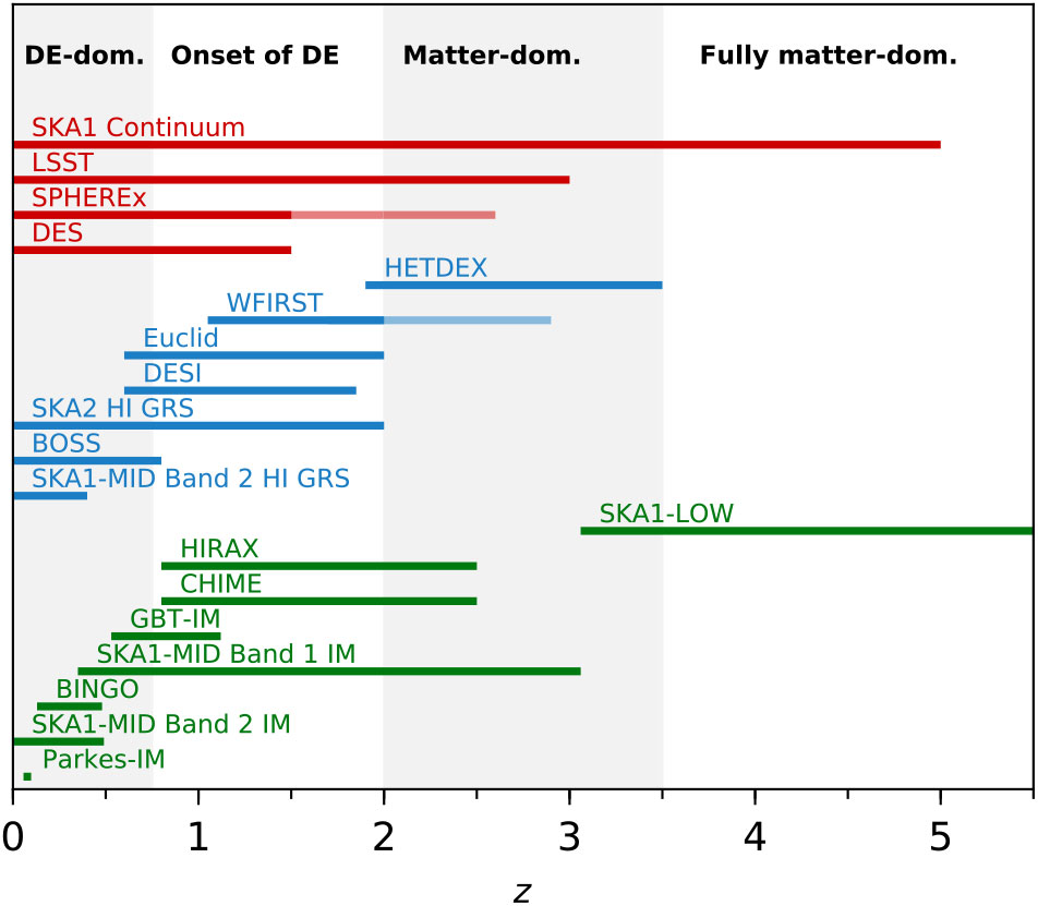
Figure 13. The approximate redshift ranges of various current and future LSS surveys. 21-cm IM surveys are shown in green (bottom), spectroscopic galaxy redshift surveys in blue (middle), and photometric/continuum surveys in red (top). WFIRST and SPHEREx both have secondary samples (with lower number density or photometric precision), which are shown as paler colours. Taken together, the SKA surveys offer full coverage of the redshift range from 0 to  $\gtrsim\! 6$, using multiple survey methods. The grey bands show an approximate division of the full redshift range into different eras, corresponding to the dark-energy-dominated regime, the onset of dark energy, the matter-dominated regime, and the fully matter-dominated regime.
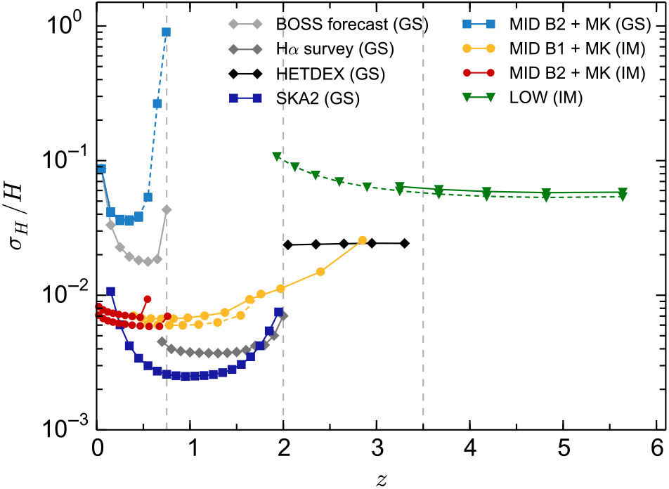
Figure 14. Forecasts for the fractional error on the expansion rate, H(z), expected to be achieved with various galaxy surveys (GS) and IM surveys, from Bull (Reference Bull2016). SKA surveys will be able to effectively survey volumes at higher redshifts than optical/NIR experiments, and with SKA2 will ultimately achieve better precision in the  $0 \lesssim z \lesssim 2$ regime as well. Figure reproduced with permission, from Reference BullBull (2016).
Secondly, SKA will be capable of detecting the BAO at significantly higher redshifts than most galaxy surveys, with SKA1-Mid Band 2. While dark energy dominates the cosmic energy density only at relatively low redshifts,  $z < 1$, many dark energy models exhibit a tracking behaviour that means that their equation of state deviates most significantly from a cosmological constant at $z \gtrsim 2-3$. Precision determinations of w(z) at $z > 2$ may therefore be more discriminating than those in the more obvious low-redshift regime that is being targeted by most spectroscopic galaxy surveys.
4.2.2. Redshift drift as a direct probe of expansion
Most probes of acceleration rely on measuring distances or the expansion rate, using standard rulers or candles. An interesting alternative is to observe the so-called redshift drift, which is the time variation of the cosmological redshift,  ${\rm d} z/{\rm d} t$ (Sandage Reference Sandage1962; Loeb Reference Loeb1998). This allows a very direct measurement of the expansion rate, as
 $$
\begin{equation}
\frac{{\rm d} z}{{\rm d} t} = (1+z)H_0 - H(z),
\label{eqn11}
\end{equation}
$$
$$
\begin{equation}
\frac{{\rm d} z}{{\rm d} t} = (1+z)H_0 - H(z),
\label{eqn11}
\end{equation}
$$and has the advantage of giving a ‘smoking gun’ signal for cosmic acceleration—the redshift drift can be positive only in accelerating cosmological models. While the existence of an apparent cosmic acceleration is well established, much of the evidence comes from probes that are interpreted in a model-dependent way, that is, within the context of a (perturbed) FLRW model. A number of non-FLRW cosmologies have been proposed in the past that appear to be accelerating when distance/expansion rate measurements are interpreted within an assumed FLRW model, but in which the expansion of space is actually decelerating locally everywhere (Clarkson & Maartens Reference Clarkson and Maartens2010; Andersson & Coley Reference Andersson and Coley2011; Bull & Clifton Reference Bull and Clifton2012). This effect is normally achieved though the introduction of large inhomogeneities, which distort the past lightcone away from the FLRW behaviour, but which still reproduce the isotropy of the Universe as seen from Earth. While this kind of model has essentially been ruled out as a possible explanation for dark energy by other observables (see e.g., Bull et al. Reference Bull, Clifton and Ferreira2012; Zibin Reference Zibin2011), the question of whether smaller inhomogeneities could cause non-negligible biases in estimates of background cosmological parameters is still very much open (e.g., Clarkson et al. Reference Clarkson2012; Bonvin et al. Reference Bonvin, Clarkson, Durrer, Maartens and Umeh2015; Fleury et al. Reference Fleury, Clarkson and Maartens2017). Redshift drift provides an independent and arguably more direct way of measuring cosmic acceleration, and so represents a promising observable for studying these effects and, eventually, definitively determining their size. The independence of redshift drift from other probes is also advantageous for breaking degeneracies in measurements of dark energy observables such as the equation of state (Martinelli et al. Reference Martinelli, Pandolf,i, Martins and Vielzeuf2012; Kim et al. Reference Kim, Linder, Edelstein and Erskine2015; Geng et al. Reference Geng, Zhang and Zhang2014).
In principle, one can measure the redshift drift effect by tracking the change in redshift of spectral line emission over some period of time. To get an estimate of the magnitude of this effect, we note that  $H_0 = 100 {\rm h}\,
{\rm km}\,{\rm s}^{-1}\,{\rm Mpc}^{-1} \sim 10^{-10}~{\rm yr}^{-1}$, so observing the redshift drift over a time baseline of
$H_0 = 100 {\rm h}\,
{\rm km}\,{\rm s}^{-1}\,{\rm Mpc}^{-1} \sim 10^{-10}~{\rm yr}^{-1}$, so observing the redshift drift over a time baseline of  $\Delta t = 10$ yr would require a spectral precision of $\Delta z \sim 10^{-9}$, corresponding to a frequency shift in, for example, the 21-cm line of $\Delta \nu \sim 1$ Hz. Plugging in exact numbers for $\Lambda$CDM, the required spectroscopic precision is actually more like 0.1 Hz if one wishes to measure the cosmic acceleration directly at $z \approx 1$ (Klöckner et al. Reference Klöckner2015). Achieving this sort of precision is challenging, as a number of systematic effects must be controlled in a consistent manner for over a decade or more. From a practical standpoint, the best way forward seems to be to perform differential measurements of the time dependence of line redshifts over many thousands, if not millions, of galaxies. SKA2 will provide the requisite sensitivity and spectral precision to perform this test for millions of HI galaxies out to $z \sim 1.5$. More details, including an examination of systematics such as peculiar accelerations, are given by Klöckner et al. (Reference Klöckner2015).
4.3. Cosmological tests of GR
GR has been exquisitely tested for a wide range in gravitational potential  $\sim GM/rc^2$ and tidal field strength
  $\sim
GM/r^3c^2$ (Psaltis Reference Psaltis2008); this includes tests in our solar system and extreme environments such as binary pulsars. Nevertheless, there is a dearth of direct tests of GR for tidal strengths
$\sim
GM/r^3c^2$ (Psaltis Reference Psaltis2008); this includes tests in our solar system and extreme environments such as binary pulsars. Nevertheless, there is a dearth of direct tests of GR for tidal strengths  $<10^{-50}$, which also happens to correspond to the domain in which we notice DM and dark energy. It is therefore of great interest to test GR in a cosmological context.
Now we turn to the other explanation for accelerated expansion: that we are mistaken about the law of gravity on very large scales. This can generate acceleration by changing the geometric part of the Einstein equation by modifying the Einstein–Hilbert action, and so requires no extra ‘dark fluid’. Many such models have been proposed (for a review, see Bull et al. Reference Bull2016), but most of these produce a expansion history similar or identical to those predicted by dark energy models. Alternative observational tests are needed to distinguish between dark energy and modified gravity, through measurement of the growth of cosmic structures.
Cosmological observations are sensitive to the effects of gravity in diverse ways. In a universe described by a perturbed FLRW metric, observations such as RSD are sensitive to the time-part of the metric, while gravitational lensing is affected by both the time-part and the space-part. These elements of the metric are themselves related to the density distribution of matter via the Einstein field equations (or classically, the Poisson equation).
A simple test of gravity, then, is to examine whether the combination of different cosmological observations behaves as expected in GR, or if a simple modification fits the observations better. If we model the Universe with a perturbed FLRW model,
 $$
\begin{equation}
{\rm d} s^2 = - (1+2\Psi){\rm d} t^2 + (1-2\Phi) a^2 {\rm d} x_i\wedge{\rm d} x^i,
\label{eqn12}
\end{equation}
$$
$$
\begin{equation}
{\rm d} s^2 = - (1+2\Psi){\rm d} t^2 + (1-2\Phi) a^2 {\rm d} x_i\wedge{\rm d} x^i,
\label{eqn12}
\end{equation}
$$ where  $\Psi$ and $\Phi$ are the two gauge-invariant Bardeen potentials and a(t) is the cosmological scale factor. We can parametrise a range of modifications to gravity by the ratio $\eta=\Psi/\Phi$, and an additional factor $\mu$ in Poisson’s equation relating $\Psi$ and overdensity. We can then calculate observables for various values of $\eta$ and $\mu$ and fit these to the cosmological probe data.
A more sophisticated approach is to write down a general action for linear cosmological perturbations of theories of gravity (e.g., Lagos et al. Reference Lagos, Baker, Ferreira and Noller2016) that contains parameters  $\alpha_i$ characterising the theories. Again, observables can be calculated for particular values of $\alpha_i$, and so the permitted range of gravity theories fitting cosmological data can be assessed.
4.3.1. Growth rate measurements with peculiar velocities
Many dark energy and modified gravity models are capable of mimicking a  $\Lambda$CDM expansion history, and so could be indistinguishable from a cosmological constant based on the equation of state of dark energy alone. This is not the case for the growth history, however, which is typically substantially modified regardless of the background evolution. This is because modifications to GR tend to introduce new operators/couplings in the action, which lead to new terms in the evolution equations with distinct redshift and scale dependences.
A useful illustration can be found in the Horndeski class of general single scalar field modifications to GR. In the sub-horizon quasi-static limit (where spatial derivatives dominate over time derivatives), the linear growth equation for matter perturbations can be written as (Baker et al. Reference Baker, Ferreira and Skordis2014a; Gleyzes Reference Gleyzes2017)
 $$
\begin{equation}
\ddot{\Delta}_M + \mathcal{H}\dot{\Delta}_M -\frac{3}{2}\Omega_M(a) \mathcal{H}^2 \xi \Delta_M = 0,
\label{eqn13}
\end{equation}
$$
$$
\begin{equation}
\ddot{\Delta}_M + \mathcal{H}\dot{\Delta}_M -\frac{3}{2}\Omega_M(a) \mathcal{H}^2 \xi \Delta_M = 0,
\label{eqn13}
\end{equation}
$$ where overdots denote conformal time derivatives,  $\mathcal{H} = a H$ is the conformal Hubble rate, $\Delta_M$ is the matter density perturbation, and $\xi(k, a) = 1$ in GR. The modification to the growth source term is restricted to have the form
 $$
\begin{equation}
\xi(k, a) = \frac{f_1(a) + f_2(a) / k^2}{f_3(a) + f_4(a) / k^2},
\label{eqn14}
\end{equation}
$$
$$
\begin{equation}
\xi(k, a) = \frac{f_1(a) + f_2(a) / k^2}{f_3(a) + f_4(a) / k^2},
\label{eqn14}
\end{equation}
$$ where  $\{\,f_n\}$ are arbitrary functions of scale factor that depend on the new terms added to the action. Within Horndeski models, all new terms in the action contribute to $\xi(k, a)$ and will cause deviations from GR growth at some scale and/or redshift. As such, we see that tests of growth can be more decisive in searching for deviations from GR than the equation of state.
The growth history can be constrained through a number of observables, for example, the redshift-dependent normalisation of the matter power spectrum, D(z), as probed by lensing or galaxy surveys; the ISW effect seen in the CMB and/or galaxy surveys, and the growth rate,  $f(z) = d\log D / d\log a$, primarily measured through probes of the cosmic peculiar velocity field. In this section, we will concentrate on the growth rate, as it exhibits fewer degeneracies with other cosmological parameters than the growth factor, D(z), and can be measured with significantly higher signal-to-noise than the ISW effect.
The most precise growth rate constraints to date come from the RSD effect, which makes the 3D correlation function of galaxies anisotropic as seen by the observer. The effect is caused by the addition of a Doppler shift to the observed redshift of the galaxies, due to the line-of-sight component of their peculiar velocities. The growth rate can only be measured in combination with either the galaxy bias, b(z), or overall normalisation of the power spectrum,  $\sigma_8$, using the RSD technique, as these terms also enter into the quadrupole (or ratio of quadrupole to monopole) of the galaxy correlation function. As discussed in Section 3.1.1.5 and by Bull (Reference Bull2016), HI galaxy redshift surveys and 21-cm IM surveys with SKA are expected to yield sub-percent level constraints on the combination $f \sigma_8$ out to $z \sim 1.7$.
The SKA will also provide a more direct measurement of the peculiar velocity field, through observations of galaxy rotation curves and the TF relation (Tully & Fisher Reference Tully and Fisher1977). The TF relation is an empirical relationship between the intrinsic luminosity of a galaxy and its rotational velocity. Assuming that it can be accurately calibrated, the TF relation can therefore be used to convert 21-cm line widths—which depend on the rotation velocity—into distances (which can be inferred from the ratio of the intrinsic luminosity and observed flux of the galaxy). Comparing the measured distance with the one inferred from the redshift of the galaxy then gives the peculiar velocity (e.g., Springob et al. Reference Springob, Masters, Haynes, Giovanelli and Marinoni2007).
This method has the disadvantage of being restricted to relatively low redshifts—the error on the velocity typically scales  $\propto
(1+z)$—and relying on a scaling relation that must be calibrated empirically. Nevertheless, direct observations of the peculiar velocity field are sensitive to the combination
$\propto
(1+z)$—and relying on a scaling relation that must be calibrated empirically. Nevertheless, direct observations of the peculiar velocity field are sensitive to the combination  $f H \sigma_8$ instead of
  $f
\sigma_8$, and so can provide complementary information to the RSD measurements (and help break parameter degeneracies). The SKA and its precursors will be able to perform suitable spectrally resolved surveys of many tens of thousands of HI galaxies out to
$f
\sigma_8$, and so can provide complementary information to the RSD measurements (and help break parameter degeneracies). The SKA and its precursors will be able to perform suitable spectrally resolved surveys of many tens of thousands of HI galaxies out to  $z\sim 0.3-0.4$ over most of the sky—essentially the widest and deepest TF velocity survey possible. As well as providing a valuable independent probe of the velocity field, these data can also be combined with the clustering information from a traditional redshift survey extracted from the same survey dataset, resulting in a significant improvement in the precision on $f\sigma_8$ compared with either probe individually (Koda et al. Reference Koda2014). A full-sky survey with SKA precursor surveys WALLABY and WNSHS should be capable of putting a joint RSD+TF constraint of $\sim 4\%$ on $f \sigma_8$ in a single $z \approx 0$ redshift bin, for example (Koda et al. Reference Koda2014).
4.3.2. Radio weak lensing
Weak lensing maps the coherent distortions of galaxy shapes across the sky (see e.g., Bartelmann & Schneider Reference Bartelmann and Schneider2001, for a review). With the path taken by light from distant galaxies determined by the matter distribution along the line of sight, and the response of curvature to that matter distribution, lensing represents an excellent probe of the theory of gravity. Dividing sources into tomographic redshift bins also allows us to track structure growth over cosmic time.
The SKA will be capable of detecting the high number densities of resolved, high-redshift star-forming galaxies over large areas necessary for weak lensing surveys (Bonaldi et al. Reference Bonaldi, Harrison, Camera and Brown2016), with expected number densities of  $\sim\! 2-3$ arcmin–2 over 5 000 deg $^2$ for SKA1 and
  $\sim
12$ arcmin–2 over 30 000 deg
$\sim
12$ arcmin–2 over 30 000 deg $^2$ for SKA2, giving comparable raw source numbers to DES and Euclid, respectively. Doing weak lensing in the radio band also has a number of distinct advantages, including the expectation of a higher-redshift source population (e.g., Brown et al. Reference Brown2015; Harrison et al. Reference Harrison, Camera, Zuntz and Brown2016) and information on intrinsic alignments from polarisation (Brown & Battye Reference Brown and Battye2011) and rotational velocity (Huff et al. 2013) information. Foremost, however, is the advantage of being able to combine weak lensing measurements between SKA and optical surveys, forming cross-power spectra $C_{\ell}^{XY}$ (where X,Y label shear measurements for the two different experiments and i,j different redshift bins):
 $$
\begin{align} C
^{X_{i}Y_{j}} _\ell = \frac{9H_0^4 \Omega_{\rm m}^2}{4c^4} \int_0^{\chi_{\rm
h}} {\rm d} \chi \, \frac{g^{X_i}(\chi) g^{Y_j}(\chi)}{a^2(\chi)} P_{\delta}
\left(\frac{\ell}{f_K(\chi)},\chi \right)\!, \label{eqn15}
\end{align}
$$
$$
\begin{align} C
^{X_{i}Y_{j}} _\ell = \frac{9H_0^4 \Omega_{\rm m}^2}{4c^4} \int_0^{\chi_{\rm
h}} {\rm d} \chi \, \frac{g^{X_i}(\chi) g^{Y_j}(\chi)}{a^2(\chi)} P_{\delta}
\left(\frac{\ell}{f_K(\chi)},\chi \right)\!, \label{eqn15}
\end{align}
$$ where  $a(\chi)$ is the scale factor of the Universe at co-moving distance $\chi$, $f_K(\chi)$ is the angular diameter distance, $P_{\delta}(k, \chi)$ is the matter power spectrum, and $g^{i}(\chi)$ are the lensing kernels.
Using only these cross-experiment power spectra to form cosmological constraints has been shown to retain almost all of the statistical power available from the intra-experiment (i.e.,  $C_{\ell}^{XX}$) power spectra (Harrison et al. Reference Harrison, Camera, Zuntz and Brown2016), while removing wavelength-dependent systematics that can otherwise cause large biases in the parameter estimation (see Camera et al. Reference Camera, Harrison, Bonaldi and Brown2017; Demetroullas & Brown Reference Demetroullas and Brown2016, for a demonstration on real data).
Figure 15 shows constraints on modified gravity parameters as specified by Dossett et al. (Reference Dossett, Ishak, Parkinson and Davis2015) (with  $R=\eta$ and $\Sigma=\mu(1+\eta)/2$ in the notation specified here for Eq. 12), showing the equivalent constraining power of both SKA-only and SKA $\times$ optical to that expected from premier optical surveys. Similar constraints are available in the $w_0-w_a$ plane, with $\sim\!30\%$ constraints available from SKA1 and $\sim\!10\%$ constraints from SKA2 (both when combined with Planck CMB measurements). Note that the empty contours do refer to the cross-correlation alone, not to the combination of radio and optical. It is clear from this, as we mentioned above, that the cross-correlations contain as much constraining power as the autocorrelations.
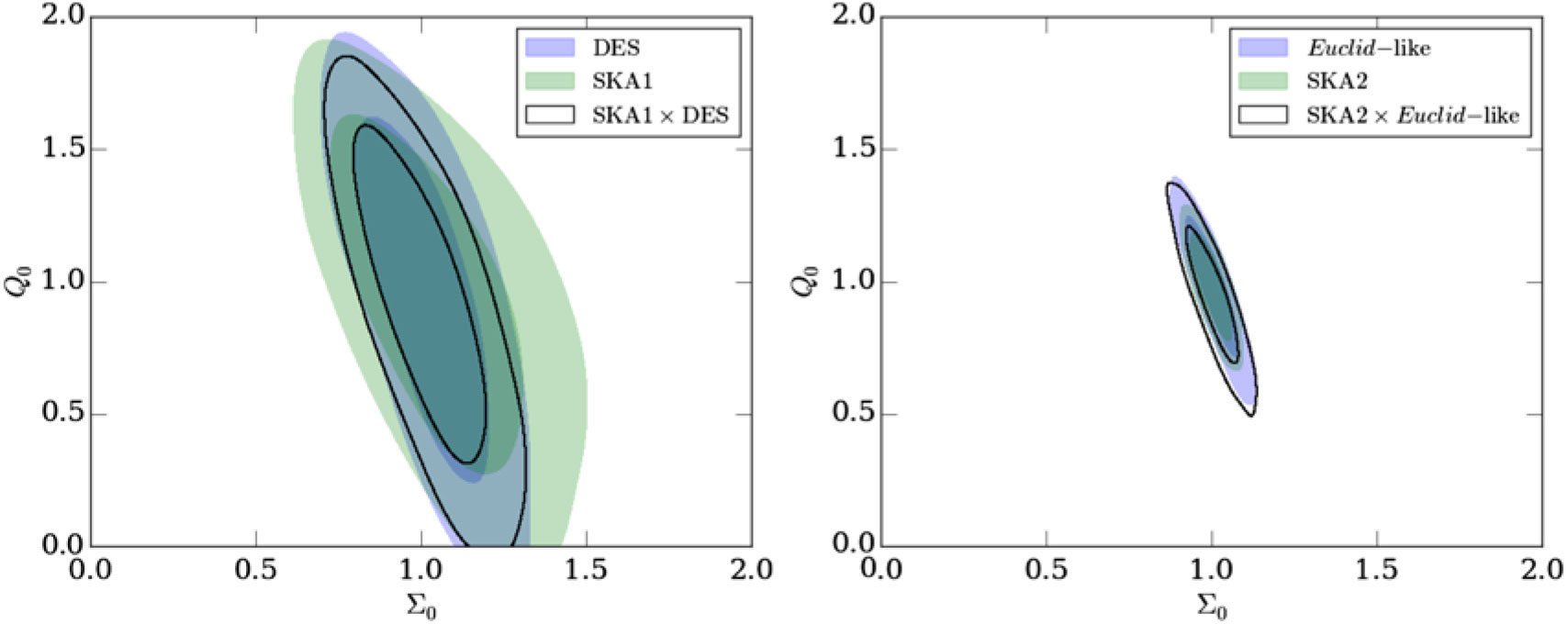
Figure 15. SKA1 (left) and SKA2 (right) constraints on modified gravity parameters as described in the text, from optical-only (blue), radio-only (green) and radio  $\times$ optical cross-correlation-only (empty contours) cosmic shear power spectrum measurements. The forecasts were created using Markov chain Monte Carlo forecasts from the CosmoSIS toolkit (Zuntz et al. Reference Zuntz2015) and are marginalised over the base $\Lambda$CDM parameters. Figure reproduced with permission, from Harrison et al. (Reference Harrison, Camera, Zuntz and Brown2016)
.
$\Lambda$CDM parameters. Figure reproduced with permission, from Harrison et al. (Reference Harrison, Camera, Zuntz and Brown2016)
.
4.3.3. Doppler magnification
Gravitational lensing consists of shear and convergence,  $\kappa$. While the shear is determined only by the matter distribution along the line of sight, the convergence also has contributions from the Doppler, Sachs–Wolfe, Shapiro time delay, and ISW effects (Bonvin Reference Bonvin2008; Bolejko et al. Reference Bolejko, Clarkson, Maartens, Bacon, Meures and Beynon2013; Bacon et al. 2014; Kaiser & Hudson Reference Kaiser and Hudson2015; Bonvin et al. 2017). These contributions modify the distance between the observer and the galaxies at a given redshift and consequently they change their observed size. The main contributions are gravitational lensing and a Doppler term: $\kappa=\kappa_{\rm g}+\kappa_{\rm v}$, where
 $$\kappa_{\rm g}=\frac{1}{2r}\int_{0}^{r} dr'\frac{r-r'}{r'}\Delta_\Omega(\Phi+\Psi)\, ,\\[3pt]
\kappa_{\rm v}=\left(\frac{1}{r\mathcal{H}} -1\right)\textbf{V}\cdot\textbf{n}\, , \nonumber%\label{kappav}$$
$$\kappa_{\rm g}=\frac{1}{2r}\int_{0}^{r} dr'\frac{r-r'}{r'}\Delta_\Omega(\Phi+\Psi)\, ,\\[3pt]
\kappa_{\rm v}=\left(\frac{1}{r\mathcal{H}} -1\right)\textbf{V}\cdot\textbf{n}\, , \nonumber%\label{kappav}$$ where  $r=r(z)$ is the co-moving distance, $\Delta_\Omega$ is the 2-sphere Laplacian which acts on the gravitational potentials $\Phi$ and $\Psi$, $\mathcal{H}$ is the conformal Hubble rate, and $\textbf{V}\cdot\textbf{n}$ is the peculiar velocity of a source projected along the line of sight $\textbf{n}$. Can we observe $\kappa_{\rm v}$? This contribution to the convergence has so far been neglected in lensing studies, but it has been shown that it can be measured in upcoming surveys (Bacon et al. 2014; Bonvin et al. 2017), and can improve parameter estimation as we now discuss. Further details are provided by Bonvin et al. (2017).
For a given object, its peculiar velocity,  $\textbf{V}$, is induced by nearby matter clustering, and so we expect the Doppler convergence to be strongly correlated with the observed galaxy number density, giving a signal in the cross-correlation $\xi=\langle \Delta(z,\textbf{n})\,\kappa(z',\textbf{n}') \rangle$. For an overdensity, objects in front of it in redshift-space will appear disproportionately larger than those behind, giving a clear dipole in $\xi$. In general, the correlation between $\Delta=b\, \delta -\frac{1}{\mathcal{H}} \partial_r(\textbf{V}\cdot\textbf{n})$, which includes local bias b(z) and an RSD term, and $\kappa_{\rm v}$, is given by
 $$
\begin{align}
&\xi_{\rm v}(r,d,\beta)=\frac{\mathcal{H}(z)}{\mathcal{H}_0}f(z)\left(1-\frac{1}{\mathcal{H}(z)r(z)} \right)\label{eqn16}\end{align}
$$
$$
\begin{align}
&\xi_{\rm v}(r,d,\beta)=\frac{\mathcal{H}(z)}{\mathcal{H}_0}f(z)\left(1-\frac{1}{\mathcal{H}(z)r(z)} \right)\label{eqn16}\end{align}
$$ $$
\begin{align}
&\quad\times\left\{\left(b(z)+\frac{3f(z)}{5}
\right)\nu_1(d)P_1(\cos\beta)-\frac{2f(z)}{5}\nu_3(d)P_3(\cos\beta)
\right\}\!, \nonumber
\end{align}
$$
$$
\begin{align}
&\quad\times\left\{\left(b(z)+\frac{3f(z)}{5}
\right)\nu_1(d)P_1(\cos\beta)-\frac{2f(z)}{5}\nu_3(d)P_3(\cos\beta)
\right\}\!, \nonumber
\end{align}
$$ where  $f={d\ln D}/{d \ln a}$ is the growth rate (D is the growth function), $P_\ell$ are the Legendre polynomials of order $\ell$, and $\nu_\ell$ is the power spectrum integrated against the $\ell$’th spherical Bessel function. $\beta$ is the angle between the points where $\Delta$ and $\kappa$ are measured with respect to the line of sight. Here, we have used the plane-parallel approximation, which makes the multipole expansion transparent— $P_1$ is a dipole and $P_3$ an octopole. The RSD contribution alters the coefficient of the second term in dipole. The correlation with RSD also induces an octopole in the $P_3$ term.
Multipole patterns in  $\xi$ can be optimally extracted by integrating against the appropriate Legendre polynomial, $P_1(\cos\beta)$ in the case of the dipole. This implies we can optimally measure Doppler magnification in a survey of volume V using the estimator
 $$\nonumber\xi_{\rm dip}(d)=\frac{3}{4\pi}\frac{\ell_p^5}{d^2V} \sum_{ij} \Delta_i \kappa_j \cos\beta_{ij}\delta_K(d_{ij}-d),\, %,\\$$
 where we associate to each pair of pixels (i, j) of size  $\ell_p$ a separation $d_{ij}$ ( $\delta_K(d_{ij}-d)$ selects pixels with separation d) and an orientation with respect to the line-of-sight $\beta_{ij}$. We measure the galaxy number count $\Delta_i$ and convergence $\kappa_j$ in each pixel, respectively. A similar estimator can be constructed for the octopole. The dipole becomes, on average in the continuous limit,
 $$
\begin{eqnarray}\nonumber
&\langle\hat{\xi}_{\rm dip}\rangle(d)\simeq\frac{\mathcal{H}(z)}{\mathcal{H}_0}f(z)\left(1-\frac{1}{\mathcal{H}(z)r(z)} \right)\left(b(z)+\frac{3f(z)}{5} \right)\nu_1(d)\, .
\end{eqnarray}
$$
$$
\begin{eqnarray}\nonumber
&\langle\hat{\xi}_{\rm dip}\rangle(d)\simeq\frac{\mathcal{H}(z)}{\mathcal{H}_0}f(z)\left(1-\frac{1}{\mathcal{H}(z)r(z)} \right)\left(b(z)+\frac{3f(z)}{5} \right)\nu_1(d)\, .
\end{eqnarray}
$$ In general, this estimator also includes a dipole contribution from the normal lensing term since objects behind overdensities are magnified, but below  $z\sim1$ it is the Doppler term which dominates, so we neglect it here.
We present an example forecast of the expected signal-to-noise for the SKA2 galaxy survey in Figure 16. We present it for a broad range of the expected error on size measurements  $\sigma_\kappa$, and we assume that an intrinsic size correlation will have a negligible dipole. For a range of separations $12\leq d \leq 180$ Mpc/h, combined over $0.1\leq z\leq 0.5$ (assuming that uncorrelated redshift bins), the cumulative signal-to-noise ratio is 35 (93) for the dipole and 5 (14) for the octopole, for $\sigma_\kappa = 0.3$ (0.8). The SKA should therefore allow a highly significant detection of the Doppler magnification dipole, and a firm detection of the octopole.
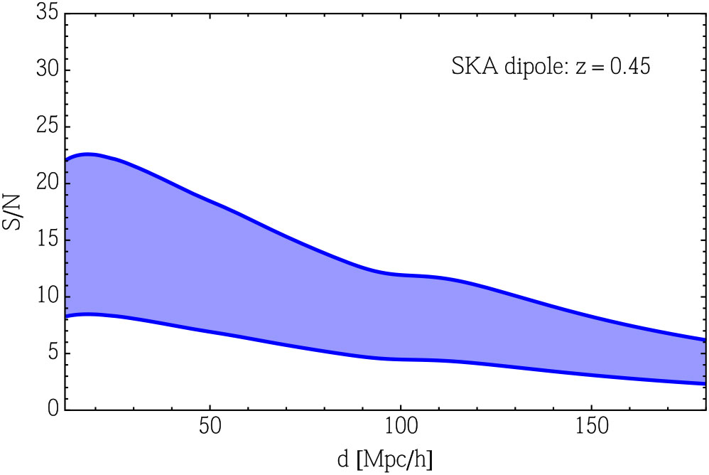
Figure 16. Signal-to-noise ratio for the Doppler magnification dipole as a function of separation, for a redshift bin  $0.4<z<0.5$ in an SKA Phase 2 HI galaxy survey. The higher bound is for an intrinsic error on the size measurement of $\sigma_\kappa=0.3$, and the lower bound is for $\sigma_\kappa=0.8$. For the octopole the signal-to-noise is about an order-of-magnitude smaller. Figure reproduced with permission, from Bonvin et al. (2017).
As an example of the improvement to parameter estimation that the Doppler dipole will give, in Figure 17 we show the constraints on  $w_0-w_a$ (marginalised over all other parameters, but fixing the bias model) from Planck (temperature, polarisation, and CMB lensing) alone, and Planck combined with an SKA2 HI galaxy survey. Comparing with constraints from RSDs (see e.g., Figure 10 of Grieb et al. Reference Grieb2017) we find that slightly better constraints are expected to be provided for the Doppler magnification dipole, while similar constraints are expected for the SKA shear measurements. This is also the case for constraints on modifications to gravity.
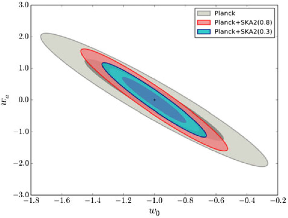
Figure 17. Joint constraints on the  $w_0$ and $w_a$ parameters, marginalised over all other parameters (except the bias, which is fixed), for Planck (T+P+lensing) alone, and Planck combined with an SKA2 HI galaxy survey. We use the dipole at separation 12 Mpc/ $h \leq d \leq$ 180 Mpc/h. Figure reproduced with permission, from Bonvin et al. (2017).
In summary, extracting the dipole of the density size cross-correlation is a novel new probe which is complementary to other lensing and RSD measurements. This will help improve constraints from the SKA2 galaxy survey. Furthermore, if we measure both the dipole and the RSD quadrupole, we can test for the scale independence of the growth rate, because the quadrupole is sensitive to the gradient of the velocity whereas the dipole is sensitive to the velocity itself. In addition, it should be possible to reconstruct the peculiar velocity field directly from measurements of the Doppler magnification dipole (Bacon et al. 2014).
4.3.4. Cross-correlations with 21-cm intensity maps
A very promising way to test dark energy and gravity with the SKA is using the HI IM technique (Santos et al. Reference Santos2015). A large sky HI IM survey with SKA1-Mid can provide precise measurements of quantities like the Hubble rate, H(z), the angular diameter distance,  $D_{\rm A}(z)$, and $f\sigma_8(z)$, which depends on how dark energy and gravity behave on large scales, across a wide range of redshifts (Bull et al. Reference Bull, Ferreira, Patel and Santos2015). A major challenge for IM experiments is foreground contamination and systematic effects. Controlling such effects becomes much easier in cross-correlation with optical galaxy surveys, since noise and systematics that are survey-specific are expected to drop out (Masui et al. Reference Masui2013a; Wolz et al. Reference Wolz2017a; Pourtsidou et al. Reference Pourtsidou, Bacon, Crittenden and Metcalf2016).
Hence, cross-correlating the IM maps with optical galaxy data is expected to mitigate various systematic effects and to lead to more robust cosmological constraints. As discussed earlier in Section 3.1.1.6, we follow Pourtsidou et al. (Reference Pourtsidou, Bacon and Crittenden2017) by considering cross-correlation of an SKA1-Mid HI IM survey with a Euclid-like optical galaxy survey, assuming an overlap  $A_{\rm sky} =
7000$ deg
$A_{\rm sky} =
7000$ deg $^2$. The results are shown in Table 1: we can expect very good measurements of the growth of structure, the angular diameter distance, and the Hubble rate across a redshift range where the effects of dark energy or modified gravity are becoming important. We note again that an additional advantage of these forecasts is that they are expected to be more robust than the ones assuming autocorrelation measurements, due to the mitigation of various systematic effects. Pourtsidou et al. (Reference Pourtsidou, Bacon and Crittenden2017) also showed that a large sky IM survey with the SKA, combined with the Planck CMB temperature maps, can detect the ISW effect with a signal-to-noise ratio $\sim\! 5$, a result competitive with Stage IV optical galaxy surveys. The detection of the ISW effect provides independent and direct evidence for dark energy or modified gravity in a flat Universe.
Another way to test the laws of gravity on large scales is using the  $E_{\rm G}$ statistic (Zhang et al. Reference Zhang, Liguori, Bean and Dodelson2007; Reyes et al. Reference Reyes, Mandelbaum, Seljak, Baldauf, Gunn, Lombriser and Smith2010; Pullen et al. 2015; Reference Pullen, Alam, He and Ho2016). In Fourier space, this is defined as
 $$
\begin{equation}
E_{\rm G}(k,z) = \frac{c^2k^2(\Phi-\Psi)}{3H^2_0(1+z)\theta(k)} ,
\label{eqn17}
\end{equation}
$$
$$
\begin{equation}
E_{\rm G}(k,z) = \frac{c^2k^2(\Phi-\Psi)}{3H^2_0(1+z)\theta(k)} ,
\label{eqn17}
\end{equation}
$$ where  $\theta \equiv \mathbf{\nabla \cdot v}/H(z)$ is the peculiar velocity perturbation field. We can construct a Fourier space estimator for $E_{\rm G}$ as (Pullen et al. Reference Pullen, Alam and Ho2015)
 $$
\begin{equation}
\hat{E}_{\rm G}(\ell,\bar{z})=\frac{c^2\hat{C}_\ell^{\rm g\kappa}}{3H^2_0\hat{C}_\ell^{\rm g\theta}} \, ,
\label{eqn18}
\end{equation}
$$
$$
\begin{equation}
\hat{E}_{\rm G}(\ell,\bar{z})=\frac{c^2\hat{C}_\ell^{\rm g\kappa}}{3H^2_0\hat{C}_\ell^{\rm g\theta}} \, ,
\label{eqn18}
\end{equation}
$$ and it can be further written as a combination of the galaxy-convergence angular cross-power spectrum  $C^{\rm g\kappa}_\ell$, the galaxy angular auto-power spectrum $C^{\rm gg}_\ell$, and the RSD parameter
  $\beta =
f/b_g$. This estimator is useful because it is galaxy bias free in the linear regime. Using HI instead of galaxies, we can use 21-cm IM clustering surveys with the SKA in combination with optical galaxy, CMB, or 21-cm lensing measurements to measure
$\beta =
f/b_g$. This estimator is useful because it is galaxy bias free in the linear regime. Using HI instead of galaxies, we can use 21-cm IM clustering surveys with the SKA in combination with optical galaxy, CMB, or 21-cm lensing measurements to measure  $\hat{E}_{\rm G}$. Pourtsidou (Reference Pourtsidou2016b) considered various survey combinations and found that very precise ( $< 1\%$) measurements can be achieved.
4.4. Tests of inflation
In the  $\Lambda$CDM model, the Universe is flat, homogeneous, and has perturbations characterised by an almost-scale-invariant power spectrum of Gaussian perturbations, generated by a period of accelerated expansion in the early Universe known as inflation (Bardeen et al. Reference Bardeen, Steinhardt and Turner1983; Mukhanov Reference Mukhanov1985; Springel et al. Reference Springel2005). This primordial power spectrum creates overdensities that we can observe through temperature anisotropies in the CMB (White & Hu Reference White and Hu1997), through brightness fluctuations in the 21-cm hydrogen line (Barkana & Loeb Reference Barkana and Loeb2001; Loeb & Zaldarriaga Reference Loeb and Zaldarriaga2004), and with the cosmological LSS, once these perturbations grow non-linear (Ma & Bertschinger Reference Ma and Bertschinger1995).
The simplest model of inflation is slow-roll inflation, in which the expansion is driven by a single minimally coupled potential-dominated scalar field with a nearly flat potential. Any deviations from such a simple model, for example, if there are multiple fields contributing to the generation of fluctuations, or some change in the couplings, will lead to modified spectrum of density perturbations that can be detected by LSS surveys. We consider two such modifications: the presence of primordial non-gaussianity and the production of PBHs.
4.4.1. Primordial non-gaussianity
Non-Gaussian distributed fluctuations in the primordial gravitational potential represent one of the so-called ‘four smoking guns of inflation’. In particular, non-standard inflationary scenarios are expected to generate a large level of non-gaussianity (see e.g., Bartolo et al. Reference Bartolo, Komatsu, Matarrese and Riotto2004; Komatsu Reference Komatsu2010; Wands Reference Wands2010). If we restrict ourselves to local-type non-gaussianity, Bardeen’s gauge-invariant potential can be written as a perturbative correction to a Gaussian random field  $\phi$, whose amplitude is parameterised by the parameter $f_{\rm NL}$, that is
 $$
\begin{equation}
\Phi=\phi+f_{\rm NL}\left(\phi^2-\langle\phi^2\rangle\right) .
\label{eqn19}
\end{equation}
$$
$$
\begin{equation}
\Phi=\phi+f_{\rm NL}\left(\phi^2-\langle\phi^2\rangle\right) .
\label{eqn19}
\end{equation}
$$ The current tightest bounds on  $f_{\rm NL}$ come from measurement of the local bispectrum of the CMB (Planck Collaboration et al. Reference Collaboration2016d), and amount to
 $$
\begin{equation}
f_{\rm NL}=0.8 \pm 5.0~(1\sigma).
\label{eqn20}
\end{equation}
$$
$$
\begin{equation}
f_{\rm NL}=0.8 \pm 5.0~(1\sigma).
\label{eqn20}
\end{equation}
$$Albeit effectively ruling out models of inflation that generate a large amount of local-type primordial non-gaussianity, Planck constraints, and even future CMB experiments are not expected to improve significantly the current bounds. This calls for new data. The CMB is localised at recombination, giving only two-dimensional information about the bispectrum and higher order. Galaxy surveys can access the distribution of matter in three dimensions, thus having access to a larger number of modes than those accessible to CMB experiments, thus delivering the next level of precision.
In the linear regime, local primordial non-gaussianity generates a scale dependence of the clustering of biased tracers of the cosmic LSS (see e.g., Dalal et al. Reference Dalal, Doré, Huterer and Shirokov2008), reading
 $$
\begin{equation}
b(z,k) = \bar{b}(z)+\Delta b(z, k),
\label{eqn21}
\end{equation}
$$
$$
\begin{equation}
b(z,k) = \bar{b}(z)+\Delta b(z, k),
\label{eqn21}
\end{equation}
$$ where the non-gaussian modification to  $\bar{b}(z)$, the scaleindependent Gaussian bias, is
 $$
\begin{equation}
\Delta b(z, k) = [\bar{b}(z)-1] f_{\rm NL}\delta_{\rm ec} \frac{3\Omega_{m}H_0^2}{c^2k^2T(k)D(z,k)}.
\label{eqn22}
\end{equation}
$$
$$
\begin{equation}
\Delta b(z, k) = [\bar{b}(z)-1] f_{\rm NL}\delta_{\rm ec} \frac{3\Omega_{m}H_0^2}{c^2k^2T(k)D(z,k)}.
\label{eqn22}
\end{equation}
$$ Here, T(k) is the transfer function (normalised such that  $T(k)\to1$ when $k\to0$), and $\delta_{\rm ec}\approx 1.45$ is the critical value of the matter overdensity for ellipsoidal collapse. Because of the $1/k^2$ dependence, such a signal for non-gaussianity is the strongest on the largest cosmic scales, which are accessible by a large area galaxy clustering survey with the SKA, using either the H i 21-cm emission (Camera et al. Reference Camera, Santos, Ferreira and Ferramacho2013a) or the radio continuum emission (Raccanelli et al. 2015; Reference Raccanelli, Shiraishi, Bartolo, Bertacca, Liguori, Matarrese, Norris and Parkinson2017) of galaxies. With the SKA2 HI galaxy redshift survey, it should be possible to reach $\sigma_{f_{\rm NL}} $ close to 1 (Camera et al. Reference Camera, Santos and Maartens2015a). Even the best next-generation galaxy surveys will not be able to bring $\sigma (\,f_{\rm NL})$ below 1, using single tracers of the matter distribution (Alonso et al. Reference Alonso, Bull, Ferreira, Maartens and Santos2015b); this represents a cosmic variance floor to the capacity of galaxy surveys with a single tracer.
The MT technique, which combines the auto- and cross-correlations of two or more tracers of the underlying cosmic structure, is able to overcome the problem of cosmic variance, thus allowing us to measure the ratio of the power spectra without cosmic variance (Seljak Reference Seljak2009). The MT technique is more effective when the bias and other features of the tracers are as different as possible. Ferramacho et al. (Reference Ferramacho, Santos, Jarvis and Camera2014) have shown that the identification of radio populations in continuum galaxy catalogues allows us to push the limit on primordial non-gaussianity below  $f_{\rm NL}=1$, in particular when redshift information for radio continuum galaxies is recovered by cross-identification with optical surveys (Camera et al. Reference Camera, Santos, Bacon, Jarvis, McAlpine, Norris, Raccanelli and Rottgering2012). Alonso & Ferreira (Reference Alonso and Ferreira2015) and Fonseca et al. (Reference Fonseca, Camera, Santos and Maartens2015) have subsequently shown that an SKA1 IM survey combined with LSST can achieve
  $\sigma (\,f_{\rm
NL})<1$. Fonseca et al. (Reference Fonseca, Maartens and Santos2017) have also shown that even the precursor MeerKAT (IM) and DES (clustering of the red and blue photometric galaxy samples, combined) can improve on the Planck constraint of Equation (21) (see Figure 18). Fonseca et al. (Reference Fonseca, Camera, Santos and Maartens2015) also illustrated how detection of primordial non-gaussianity is tightly related to other relativistic effects important on the scale of the horizon. Failure in properly accounting for all these ultra-large scale corrections may lead to biased results in future cosmological analyses (Camera et al. Reference Camera, Maartens and Santos2015b,c).
$\sigma (\,f_{\rm
NL})<1$. Fonseca et al. (Reference Fonseca, Maartens and Santos2017) have also shown that even the precursor MeerKAT (IM) and DES (clustering of the red and blue photometric galaxy samples, combined) can improve on the Planck constraint of Equation (21) (see Figure 18). Fonseca et al. (Reference Fonseca, Camera, Santos and Maartens2015) also illustrated how detection of primordial non-gaussianity is tightly related to other relativistic effects important on the scale of the horizon. Failure in properly accounting for all these ultra-large scale corrections may lead to biased results in future cosmological analyses (Camera et al. Reference Camera, Maartens and Santos2015b,c).
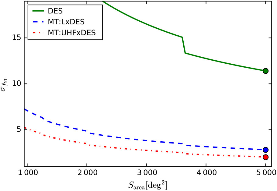
Figure 18. Constraints on  $\sigma (f_{\rm NL})$ against sky area for DES on its own (solid, green) and for MT of DES and MeerKAT (dashed, blue: low-redshift band, dot-dashed, red: high-redshift band). This calculation considers estimates for the full photometric sample of DES, that is, ‘red’ early type galaxies with ‘blue’ galaxies full of young stars. Figure reproduced with permission, from Fonseca et al. (Reference Fonseca, Maartens and Santos2017).
4.4.2. Primordial BHs
It is customary to parametrise deviations from perfect scale invariance by a few variables, which capture the change in the shape of the power spectrum at some pivot scale  $k_*$. The first of these numbers is the scalar tilt $(1-n_s)$, which expresses a constant offset in the power-law index. Higher derivatives, or runnings, of the power spectrum, are the scalar $\alpha_s=\mathrm d n_s/\mathrm d \log k$, and the second running $\beta_s\equiv\mathrm d \alpha_s/\mathrm d \log k $.
The scalar perturbations,  $\zeta_{\bf k}$, have a two-point function given by
 $$
\begin{equation}
{\zeta_{\bf k}^{}\zeta_{\bf k'}^*} = P_{\zeta}(k) (2\pi)^3 \delta_D(\bf k+k'),
\label{eqn23}
\end{equation}
$$
$$
\begin{equation}
{\zeta_{\bf k}^{}\zeta_{\bf k'}^*} = P_{\zeta}(k) (2\pi)^3 \delta_D(\bf k+k'),
\label{eqn23}
\end{equation}
$$ where  $P_\zeta(k)$ is the scalar power spectrum, for which we can define an amplitude as
 $$
\begin{align}
\log \Delta^2_s(k) &\equiv \log \left[\dfrac{k^3}{2\pi^2} P_\zeta(k) \right] = \log A_s + (n_s-1) \log\left(\dfrac k {k_{*}}\right) \nonumber \\[4pt] &\quad\qquad + \frac 1 2 \alpha_{s} \log^2\left(\dfrac k {k_{*}}\right)+ \frac 1 6 \beta_s \log^3\left(\dfrac k {k_*}\right),
\label{eqn24}\end{align}
$$
$$
\begin{align}
\log \Delta^2_s(k) &\equiv \log \left[\dfrac{k^3}{2\pi^2} P_\zeta(k) \right] = \log A_s + (n_s-1) \log\left(\dfrac k {k_{*}}\right) \nonumber \\[4pt] &\quad\qquad + \frac 1 2 \alpha_{s} \log^2\left(\dfrac k {k_{*}}\right)+ \frac 1 6 \beta_s \log^3\left(\dfrac k {k_*}\right),
\label{eqn24}\end{align}
$$ where  $A_s$ is the scalar amplitude. At the pivot scale of $k_*=0.05$ Mpc–1, Planck has measured a scalar amplitude
  $A_s = 2.092 \times
10^{-9}$, with tilt
$A_s = 2.092 \times
10^{-9}$, with tilt  $n_s=0.9656$ (Planck Collaboration et al. Reference Collaboration2018).
The primordial perturbations,  $\zeta$, generated during inflation, create matter overdensities $\delta\equiv \rho/\bar \rho -1$, where $\rho$ is the energy density and $\bar{\rho}$ its spatial average. These matter perturbations source the temperature fluctuations in the CMB and later on grow to seed the LSS of the universe. In linear theory, matter and primordial perturbations are related to each other through a transfer function $\mathcal T(k)$, so that the matter power spectrum is
 $$
\begin{equation}
P_{\delta} (k) = \mathcal T^2(k) P_{\zeta}(k).
\label{eqn25}
\end{equation}
$$
$$
\begin{equation}
P_{\delta} (k) = \mathcal T^2(k) P_{\zeta}(k).
\label{eqn25}
\end{equation}
$$ In single-field slow-roll inflation, scale invariance is predicted to extend over a vast range of scales (Baumann Reference Baumann2009; Planck Collaboration et al. Reference Collaboration2016e). However, we only have access to a small range of wavenumbers around the CMB pivot scale  $k_*=0.05$ Mpc-1. The amplitude, $A_s$, of the (scalar) power spectrum and its tilt, $n_s$, give us information about the first two derivatives of the inflaton potential when this scale, $k_*$, exited the horizon during inflation. Higher-order derivatives of this potential produce non-zero runnings, which for slow-roll inflation generically have values $\alpha_s\sim(1-n_s)^2$ and $\beta_s\sim(1-n_s)^3$, beyond the reach of present-day cosmological experiments (Adshead et al. Reference Adshead, Easther, Pritchard and Loeb2011). Next-generation cosmological experiments, including SKA galaxy surveys and 21-cm measurements, can measure these numbers.
Slow-roll inflation models generally predict  $|\alpha_{\rm s}| \sim 0.001$ and $|\beta_{\rm s}|\sim 10^{-5}$. Any large deviation from these values would disfavour single-field inflation models. Pourtsidou (Reference Pourtsidou2016a) showed that combining a Stage IV CMB experiment with a large sky 21-cm IM survey with SKA2-Mid can yield $\sigma (\alpha_{\rm s}) \simeq 0.002$, while a high-redshift ( $3<z<5$) IM survey with a compact SKA2-Low-like instrument gives $\sigma (\alpha_{\rm s}) \simeq 0.0007$. Reaching the required precision on the second running, $\beta_{\rm s}$, is difficult and can only be achieved with very futuristic interferometers probing the Dark Ages (Muñoz et al. Reference Muñoz, Kovetz, Raccanelli, Kamionkowski and Silk2017).
A detection of  $\alpha_s$, or $\beta_s$, would enable us to distinguish between inflationary models with otherwise equal predictions and would shed light onto the scalar power spectrum over a wider k range.
In the absence of any salient features in the power spectrum, such as small-scale non-gaussianities, the power in the smallest scales will be determined by the runnings of the scalar amplitude. This is of particular importance for PBH production in the early universe, where a significant increase in power is required at the scale corresponding to the PBH mass, which is of order  $k \sim 10^5$ Mpc-1 for solar mass PBHs (Green & Liddle Reference Green and Liddle1999; Carr Reference Carr2005). It has been argued that a value of the second running $\beta_s = 0.03$, within 1 $-\sigma$ of Planck results, can generate fluctuations leading to the formation of $30\,{\rm M}_{\odot}$ PBHs if extrapolated to the smallest scales (Carr et al. Reference Carr, Kühnel and Sandstad2016).
Combining galaxy-clustering SKA measurements with future CMB experiments will enhance measurements of these parameters, so that we will be able to measure significant departures from single-field slow-roll inflation. Moreover, long baseline radio interferometers observing the EoR will be able to measure the running  $\alpha_s$ with enough precision to test the inflationary prediction. However, to reach the sensitivity required for a measurement of $\beta_s\sim 10^{-5}$, a Dark Ages interferometer, with a baseline of $\sim\! 300$ km, will be required.
A large positive value of the second running,  $\beta_s$, has consequences for PBH formation. There has been interest in PBHs as a DM candidate (see e.g., Carr & Hawking Reference Carr and Hawking1974; Meszaros Reference Meszaros1974; Carr et al. Reference Carr, Kühnel and Sandstad2016), since they could explain some of the GW events observed by the LIGO collaboration (Abbott et al. Reference Abbott2016b; Bird et al. Reference Bird, Cholis, Muñoz, Ali-Haïmoud, Kamionkowski, Kovetz, Raccanelli and Riess2016).
If they are to be the DM (see Section 5.3.6.4 for a full discussion of this possibility), PBHs could have formed in the primordial universe from very dense pockets of plasma that collapsed under their own gravitational pull. The scales in which stellar mass PBHs were formed are orders of magnitude beyond the reach of any cosmological observable. However, if the inflationary dynamics were fully determined by a single field, one could extract information about the potential  $V(\phi)$ at the smallest scales from $V(\phi_*)$ at the pivot scale (and its derivatives) by extrapolation.
The formation process of PBHs is poorly understood (Green & Liddle Reference Green and Liddle1999), so one can as a first approximation assume that PBHs form at the scale at which  $\Delta_s^2(k)$ becomes of order unity. It is clear that any positive running, if not compensated by a negative running of higher order, will create enough power in some small enough scale to have $\Delta_s^2(k)=1$. Nonetheless, the mass of the formed PBHs is required to be larger than $\sim\! 10^{15}$ g (i.e., $\sim10^{-18} \, {\rm M}_{\odot}$), to prevent PBH evaporation before $z=0$, which sets a limit on the smallest scale where PBHs can form of $\sim 10^4$ km.
In order to produce PBHs of  $\sim 30 \, {\rm M}_{\odot}$, as suggested by Bird et al. (Reference Bird, Cholis, Muñoz, Ali-Haïmoud, Kamionkowski, Kovetz, Raccanelli and Riess2016) to be the DM, the relevant scale is
  $\sim\!
10$ pc. This would force the second running to be as large as
$\sim\!
10$ pc. This would force the second running to be as large as  $\beta_s \approx 0.03$, which will be tested at high significance by SKA2 galaxy surveys and IM measurements.
Detailed investigations of constraints on inflationary parameters related to PBH production and observational constraints have been performed recently, by authors including Young & Byrnes (Reference Young and Byrnes2015), Young et al. (Reference Young, Regan and Byrnes2016), Cole & Byrnes (Reference Cole and Byrnes2018), Germani & Prokopec (Reference Germani and Prokopec2017), Muñoz et al. (Reference Muñoz, Kovetz, Dai and Kamionkowski2016), Pourtsidou (Reference Pourtsidou2016a), Sekiguchi et al. (Reference Sekiguchi, Takahashi, Tashiro and Yokoyama2018). We refer to those papers for accurate and thorough observational constraints and predictions.
4.5. Tests of fundamental hypotheses
4.5.1. Tests of the Cosmological Principle
Testing the foundations of the standard cosmological model is an important part of strengthening the status of this model. One of the basic pillars of cosmology is the large-scale FLRW geometry, in other words, the cosmological principle: on large enough scales the universe is on average spatially homogeneous and isotropic. This principle consists of two parts:
Statistical isotropy of the Universe around us: There is a large body of separate evidence that the Universe is isotropic, on average, on our past lightcone. The strongest such evidence comes from the observed level of anisotropies of the CMB. The observed dipole in the CMB is consistent with our proper motion with respect to the CMB rest frame (see Kogut et al. Reference Kogut1993; Aghanim et al. Reference Aghanim2014). Thus, once corrected for this proper motion, the CMB does indeed appear isotropic around us to one part in  $10^{5}$, a level perfectly consistent with the standard model of cosmology supplemented by small fluctuations generated early during a phase of inflation. In addition, a generic test of Bianchi models presented by Saadeh et al. (Reference Saadeh, Feeney, Pontzen, Peiris and McEwen2016) with CMB strongly disfavours large-scale anisotropic expansion.
The Copernican Principle: We are typical observers of the Universe; equivalently: we are not at a special spatial location in the Universe. Relaxation of this principle has sometimes been invoked as a solution to the dark energy problem (see e.g., Garcia-Bellido & Haugboelle Reference Garcia-Bellido and Haugboelle2008; February et al. Reference February, Larena, Smith and Clarkson2010), but studies of kinetic Sunyaev–Zeldovich effects have strongly disfavoured such solutions; see Bull et al. (Reference Bull, Clifton and Ferreira2012) and Clifton et al. (Reference Clifton, Clarkson and Bull2012a). However, the principle itself remains to be tested accurately, irrespective of the actual solution to the dark energy problem.
It is clear that these two ingredients, which, when combined, imply the cosmological principle, have different scientific statuses. On the one hand, the observed statistical isotropy around us is easily constrained by direct observations down our past lightcone. On the other hand, the Copernican Principle provides a prescription about what happens off our past lightcone, both in our causal past and outside of our causal past. Assessing its validity is therefore much more difficult.
One can find detailed accounts of various ways one can constrain the large-scale geometry of the Universe from observations in two recent reviews (Clarkson & Maartens Reference Clarkson and Maartens2010; Clarkson Reference Clarkson2012). Some detailed discussions of the prospects of the SKA for future tests of the cosmological principle are presented by Schwarz et al. (Reference Schwarz2015). In particular, the SKA will be ideal to measure the cosmic radio dipole and to test if it aligns with the CMB dipole, as it should be the case in standard cosmology. A recent analysis of the WISE-2MASS optical catalogue by Bengaly et al. (Reference Bengaly, Bernui, Alcaniz, Xavier and Novaes2017) has not found any significant anisotropy in the LSS distribution, but the SKA will allow us to pinpoint the direction and amplitude of the dipole with great accuracy (e.g., with SKA2, one will be able to determine the direction of the dipole to within 1 $^\circ$; see Schwarz et al. Reference Schwarz2015), and to compare them directly with the CMB measurement, since the SKA will probe a super-horizon size volume.
Tests of the Copernican Principle, on the other hand, are much harder to design, and are usually much less precise. However, two promising techniques have emerged, which allow one to get some information on what happens off our past lightcone. First, a direct comparison of the transverse and radial scales of BAOs gives one access to a test of possible anisotropies in the local expansion rate of the Universe away from us (see Maartens Reference Maartens2011; February et al. Reference February, Clarkson and Maartens2013).
Second, direct measurements of the redshift-drift, while a remarkable probe of the nature of dark energy (see Section 4.2.2), can also help constrain the Copernican Principle, as presented by Bester et al. (Reference Bester, Larena and Bishop2015, Reference Bester, Larena and Bishop2017). Bester et al. (Reference Bester, Larena and Bishop2017) use a fully relativistic way of reconstructing the metric of the Universe from data on our past lightcone, with a minimal set of a priori assumptions on the large-scale geometry. Focusing on spherically symmetric (isotropic) observations around a central observer (in the  $\Lambda$-Lemaître-Tolman-Bondi class), one can characterise any departure from homogeneity by the scalar shear of the cosmological fluid, $\sigma^{2}=\frac{1}{2}\sigma_{ij}\sigma^{ij}$. Figure 19 presents constraints on this shear from current optical data (label $\mathcal{D}_{0}$), and for a forecast with radio astronomy data (labels $\mathcal{D}_{1}$ and $\mathcal{D}_{2}$) generated around a fiducial $\Lambda$CDM model. $\mathcal{D}_{0}$ uses Type Ia supernova data from Suzuki et al. (Reference Suzuki2012) to determine the angular distance D(z), cosmic chronometre data from Moresco et al. (Reference Moresco, Jimenez, Cimatti and Pozzetti2011); Moresco (Reference Moresco2015) to determine the longitudinal expansion rate $H_{\|} (z)$, and stellar ages from Sneden et al. (Reference Sneden, McWilliam, Preston, Cowan, Burris and Armosky1996) to put a lower bound on the age of the Universe $t_{0}$. $\mathcal{D}_{1}$ uses only Type Ia supernova data from Suzuki et al. (Reference Suzuki2012) and forecast for SKA2 BAO in IM for D(z), as well as forecast for a redshift drift experiment like Canadian Hydrogen Intensity Mapping Experiment (CHIME), from Yu et al. (Reference Yu, Zhang and Pen2014). Finally, $\mathcal{D}_{2}$ consists of all the combined inputs of $\mathcal{D}_{0}$ and $\mathcal{D}_{1}$. Details of the methods are presented by Bester et al. (Reference Bester, Larena and Bishop2017) and references therein. One clearly sees that the redshift drifts are the best data to improve on current constraints.
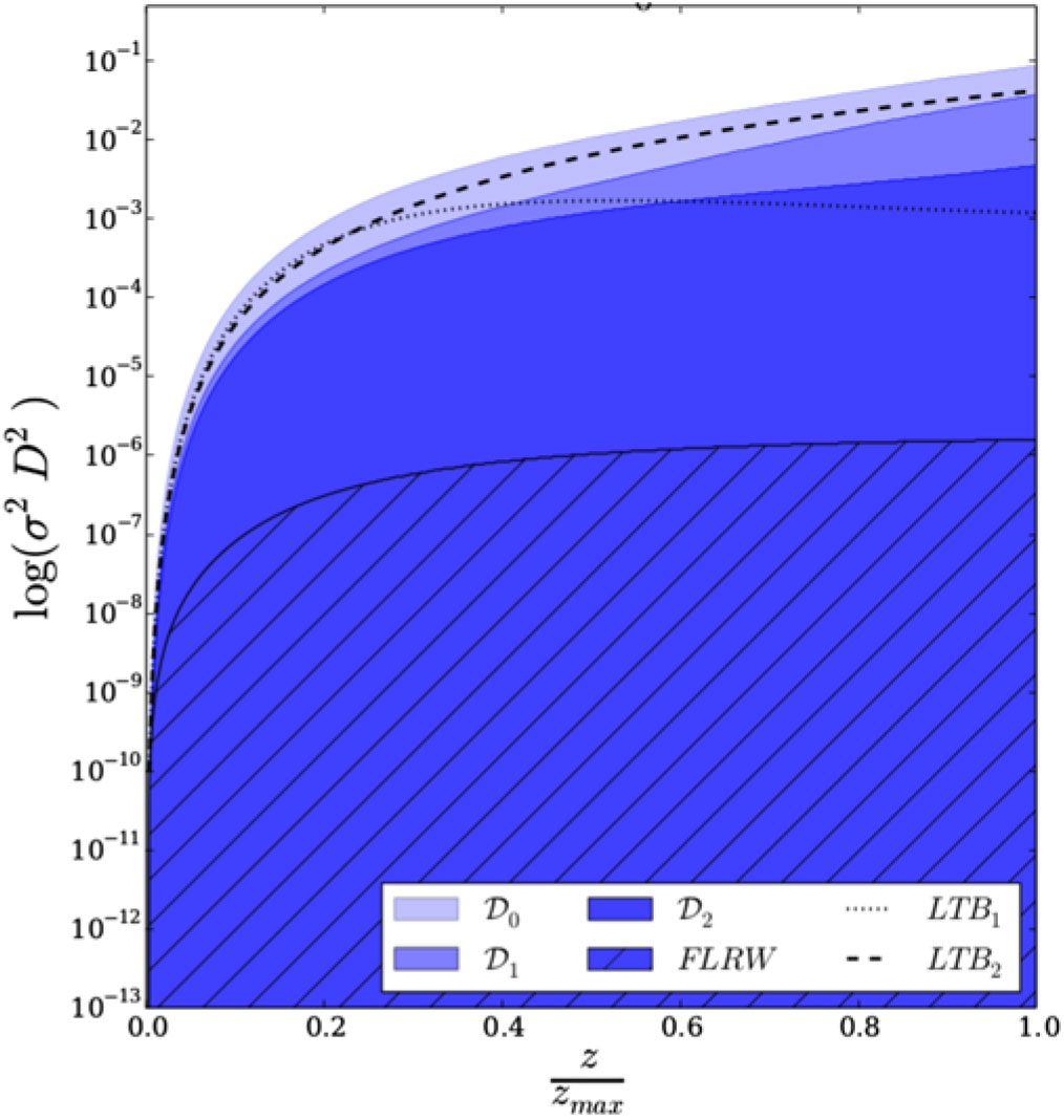
Figure 19. Constraints on the matter shear normalised by the angular distance, D, as a function of redshift on our current past lightcone. The blue regions, from light to dark, correspond to the upper 2- $\sigma$ contours reconstructed from currently available data (i.e., simulation $\mathcal{D}_{0}$), forecast, D(z) and redshift-drift data (i.e., simulation, $\mathcal{D}_{1}$) and finally all of the above, including H(z) data from longitudinal BAO measurements (i.e., simulation, $\mathcal{D}_{2}$). The hatched region corresponds to the intrinsic shear present in a perturbed FLRW model with a uv-cutoff of 100 Mpc. For comparison we also show two spherically symmetric but inhomogeneous models, one with a homogeneous bang time $t_{B}(r)=0$ (labelled LTB $_1$) and one without (labelled LTB $_2$).
Besides, they also allow for a remarkable determination of the value of the cosmological constant without assuming the Copernican Principle: as shown in Figure 20, in the class of spherically symmetric, but inhomogeneous models, the inclusion of redshift drift data allows one to constrain  $\Omega_{\Lambda}$ at less that 10%.
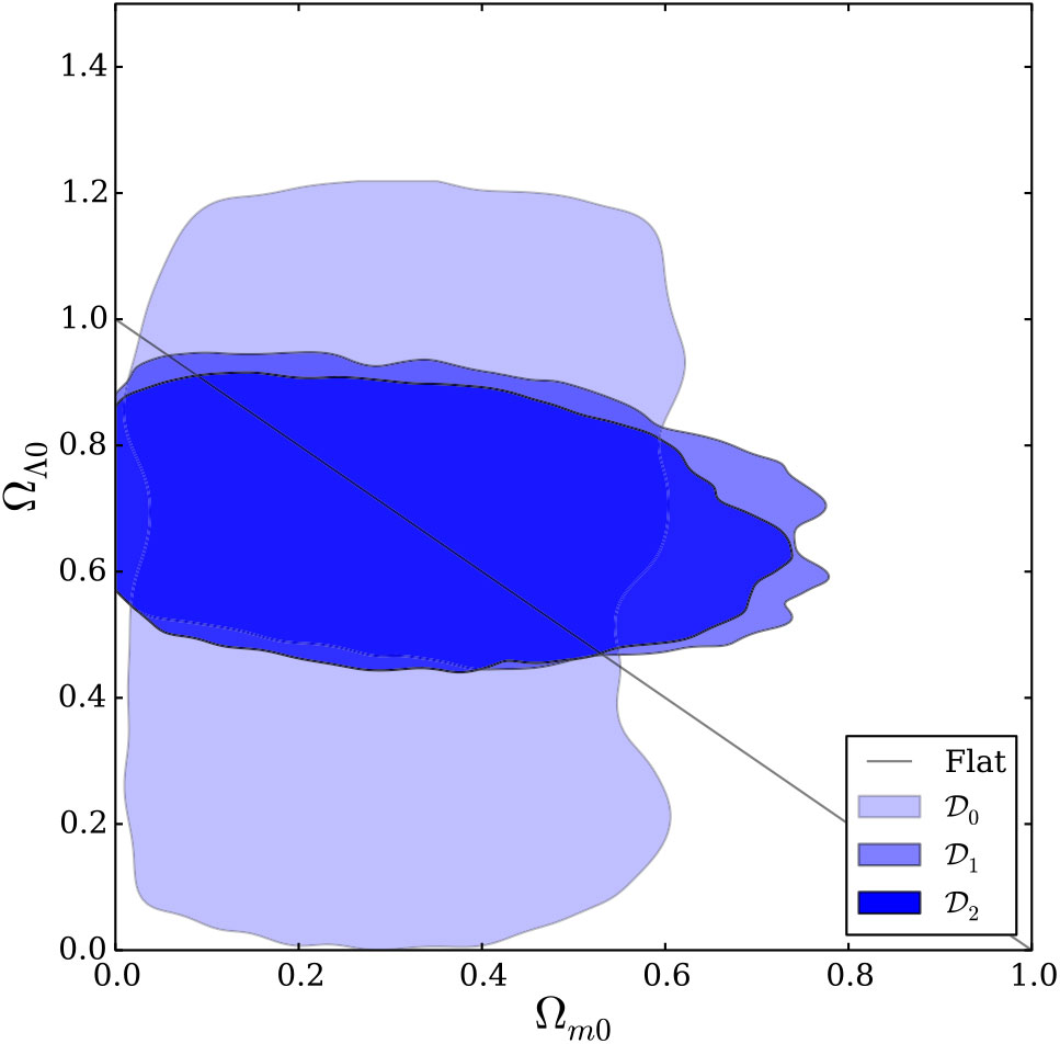
Figure 20. 2- $\sigma$ constraints on $\Omega_{\Lambda}$ and $\Omega_{m}$ on the worldline of the central observer today for the various combinations of data presented in the text.
4.5.2. Tests of LLI
Cosmological models inspired from fundamental theories may lead to violation of LLI. The strongest constraints on such proposals will be set by pulsar experiments, as discussed in Section 3.1.1.1. These constraints are proportional to the timing precession of binary pulsars, and hence will be dramatically improved with the SKA project.
A cosmological model that leads to LLI violation and has so far passed all other tests is the D-material Universe (Elghozi et al. Reference Elghozi, Mavromatos, Sakellariadou and Yusaf2016), a model which may appear as the low-energy limit of certain brane theories (Mavromatos & Sakellariadou Reference Mavromatos and Sakellariadou2007) in the context of string theories with large extra dimensions. This cosmological model aims at providing a justification for the phenomenological  $\Lambda$CDM model, which relies on the existence of two unknown quantities, namely a positive cosmological constant, $\Lambda$, and CDM component, both introduced in order to fit current astrophysical data.
According to string theory, matter consists of one-dimensional objects, the strings. Different vibrations of a string represent different particle types, while splitting and joining of elementary strings represent particle interactions. String ends live on a surface that can be thought of as a large massive object, a Dirichlet brane (D-brane), in spacetime. Branes of different dimensionality, depending on the particular string theory, are thought to be embedded within a higher dimensionality background, the bulk. In this framework, let us consider a compactified (3+1)-dimensional brane propagating in a higher dimensional bulk populated by zero-dimensionality (point-like) D-branes, called D-particles, since they have all their spatial dimensions wrapped around compact space. As the (3+1)-dimensional brane moves in the bulk, D-particles cross it, resulting in foamy structures. Since branes are by definition the collection of the end points of open strings, particle excitations (described by open strings) propagate in a medium of D-particles. Thus, brane-puncturing massive D-particles can be captured by electrically neutral matter open strings, a process that is described by the Dirac-Born-Infeld action. This scenario leads to a bi-metric theoryFootnote j (Mavromatos & Sakellariadou Reference Mavromatos and Sakellariadou2007), with a vector field appearing naturally as the result of the recoil velocity field of D-particles. The recoil results in a metric deformation of the neighbouring spacetime, and in Lorentz invariance being locally broken. The latter implies the emergence of vector-like excitations that can lead to an early era of accelerated expansion, in the absence of an inflaton field, and contribute to LSS (enhancing the DM component) and galaxy formation (Ferreras et al. Reference Ferreras, Sakellariadou and Yusaf2008, Reference Ferreras, Mavromatos, Sakellariadou and Yusaf2009; Mavromatos et al. Reference Mavromatos, Sakellariadou and Yusaf2009). The D-material universe has been shown to be in agreement with gravitational lensing phenomenology (Mavromatos et al. Reference Mavromatos, Sakellariadou and Yusaf2013). Moreover, the medium of D-particles leads to recoil velocity field condensates that induce an effective mass for the graviton (Elghozi et al. Reference Elghozi, Mavromatos and Sakellariadou2017), in agreement with the constraints imposed from the Advanced LIGO interferometric data (Abbott et al. Reference Abbott2016a,b; Abbott et al. Reference Abbott2017). So far, the D-material universe is in agreement with observational constraints (Mavromatos et al. Reference Mavromatos, Sakellariadou and Yusaf2013; Elghozi et al. Reference Elghozi, Mavromatos and Sakellariadou2017).
This, so far successful, cosmological model with the advantage of being based on a microscopic theory, can be further tested with the SKA (Janssen et al. Reference Janssen2015). LLI violation leads to modifications of the orbital dynamics of binary pulsars, as well as to modifications of the spin evolution of solitary pulsars (Shao et al. Reference Shao, Caballero, Kramer, Wex, Champion and Jessner2013), while for the latter it also leads to a spin precession with respect to a fixed direction (Shao & Wex Reference Shao and Wex2012). Hence, LLI violation implies changes in the time derivative of the orbital eccentricity, of the projected semi-major axis, and of the longitude of the periastron, while it changes the time behaviour of the pulse profile.
Since the accuracy of timing precession of binary pulsars will be significantly improved with the SKA project, one expects to further constrain models leading to LLI violation, such as the cosmological model mentioned above. For a given pulsar, the timing precision scales with the signal-to-noise ratio of its pulse profile. As simulations have indicated, if the SKA improves the signal-to-noise ratio of pulse profiles by a factor of 10, the Lorentz-violating coefficients will be constrained by the same factor, within only a 10-yr cycle of observations. Combining these SKA observations with 20 yr of pre-SKA data, one may be able to constrain the Lorentz-violating coefficients up to a factor of 50 (Shao et al. Reference Shao2015).
4.6. Summary
In this section, we have reviewed how data from the SKA will open a new era for radio cosmology, allowing us to test the foundations of the concordance cosmological model to unprecedented accuracy. Furthermore, we argue that the SKA’s commensality with other observational campaigns, aimed at scrutinising the Universe’s LSS in the optical and NIR bands, will allow us to have independent checks of crucial cosmological observations, de facto reinforcing statistical analyses on long-standing problems such as the nature of dark energy or the validity of GR on cosmological scales.
Below, we list the main points considered in the section:
• Tests of cosmic acceleration (see Section 4.2). The zeroth-order test to understand whether the late-time cosmic expansion is truly due to a cosmological constant term or if it is a dark energy component that dominates the Universe’s present-day evolution is to check the constancy of the equation of state of dark energy, w(z). The SKA will be able to do this both at the level of background and cosmological perturbations. The latter will be achieved mostly via BAO measurements, for which 21-cm IM will represent a unique added value of the SKA, compared to usual galaxy surveys. The former is envisaged through measurements of the redshift drift, which will allow us to probe the Hubble parameter directly and not as an integrated quantity, for example, as for type Ia supernovae.
• Tests of gravity ( Section 4.3). Although GR has been tested to exquisite precision in the solar system and in strong gravity regimes, we still extrapolate it for orders of magnitude when we use it to interpret cosmological data. For this reason, the possibility of deviations from Einsteinian gravity is particularly interesting in the context of dark energy, for which a modified gravity model may represent a viable alternative. The main means by which the SKA will test this hypothesis is the study of the growth of LSS. On the one hand, the SKA will complement optical/NIR surveys such as those to be performed by Euclid or LSST in quantifying deviations from GR at the level of the matter power spectrum, employing 21-cm IM, HI and continuum galaxy number counts, as well as radio weak lensing cosmic shear. On the other hand, the SKA depth and sky area will allow us to probe for the first time the largest cosmic scales, which see the peak of as-yet-undetected relativistic effects.
• Tests of inflation (Section 4.4). Those same extremely large scales where relativistic effects hide also retain pristine information about inflation. One of the most robust predictions of inflation is a certain amount of non-gaussianity in the distribution of primordial density fluctuations. By probing the growth of structures on the scale of the horizon and, in particular, by cross-correlating multiple tracers of the underlying DM distribution, we will be able to push the limits on primordial non-gaussianity, eventually reaching sub  $f_{\rm NL}=1$ precision. Moreover, the study of the matter power spectrum over a wide range of scales will allow us to test the hypothesis of PBHs, for which a significant increase in power is required at the scale corresponding to the PBH mass.
• Tests of the cosmological principle (Section 4.5.1). By measuring the cosmic radio dipole and comparing it to the observed CMB dipole, the SKA is ideally suited to test the hypothesis of statistical isotropy of the Universe around us. Furthermore, redshift drift measurements can also help to constrain the Copernican Principle, in particular by putting strong bounds on inhomogeneous cosmological models, such as  $\Lambda$-Lemaître–Tolman–Bondi cosmologies.
5. DM and astroparticle physics
5.1. Introduction
The detection of DM remains a key goal of modern cosmology and astrophysics. After three decades of searching, the case for its existence remains stronger than ever, with measurements from Planck Collaboration et al. (Reference Collaboration2018) reinforcing the hypothesis that massive, non-luminous matter comprises 26% of the total energy density of the Universe. Radio astronomy in particular has played a critical role in constraining the properties and evolution of DM halos since their initial prediction, particularly in the observation of HI rotation curves well beyond the optical radius of galaxies (see e.g., Bosma Reference Bosma1981a,b; van Albada et al. Reference van Albada, Bahcall, Begeman and Sancisi1985; Begeman Reference Begeman1989). Future radio observations may also be crucial for identifying the DM among the many suggested candidates. Weakly interacting massive particles (WIMPs) have been a primary focus, a category of new, principally fermionic, particles predicted from extensions to the standard model of particle physics. However, attention has also turned to a variety of other candidates: recent observations at LIGO (Bird et al. Reference Bird, Cholis, Muñoz, Ali-Haïmoud, Kamionkowski, Kovetz, Raccanelli and Riess2016) have re-invigorated the search for PBHs, and the search for axions has received significant support in recent years (see Figure 21 and Park Reference Park2007, for an overview of the DM parameter space).
The development of the SKA marks a significant advancement in radio astronomy and offers the possibility of direct or indirect detection of DM. One of the major challenges in doing this is to disentangle the DM signal from astrophysical signals. With its huge improvement in sensitivity, resolution, and versatility, the SKA will massively increase our understanding of astrophysical backgrounds and facilitate disentanglement. Our key goal in compiling this work is to bring together the areas in which the SKA and its precursors can make its the greatest contribution to both cosmology and particle physics. Section 5.2 looks at ways the SKA may help to constrain general DM properties; Section 5.3 reviews the search for DM candidates and details ways in which the SKA can support the search for WIMPs, axions and PBHs in particular; and Section 5.4 investigates ways in which the SKA can constrain astroparticle properties.
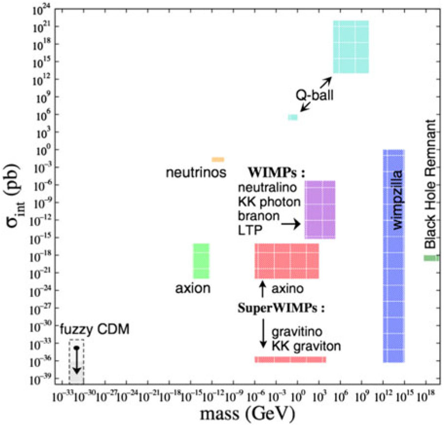
Figure 21. The mass and cross section (in picobarns, where 1 pb  $=10^{-40}$ m-2) for various DM particle candidates. Figure taken from Park (Reference Park2007).
5.2. DM properties
The evidence for DM on galaxy scales comes from 21-cm line observations of rotation curves, which do not decline beyond the optical image of gas-rich galaxies. However, it is still debated how predominant the DM is in the inner parts of such galaxies, since the mass models are degenerate, so that additional dynamical criteria have to be brought to bear. These are not straightforward, and a debate is ongoing on the validity of using stellar velocity dispersions to settle this issue (see e.g., Bosma Reference Bosma, Knapen, Lee and Gil de Paz2017, and references therein).
Attempts to constrain the geometrical shape of the DM halo, using the flaring of the HI layer beyond the optical radius, are also unexpectedly difficult. For bright galaxies, the current picture is rapidly changing, as there is more and more evidence for a complicated baryon cycle, with both accretion and outflows related to star formation activity. This affects the kinematics of extraplanar HI gas, which rotates slower than the HI in the stellar disc (e.g., Oosterloo et al. Reference Oosterloo, Fraternali and Sancisi2007, for NGC 891). Of course, smaller galaxies could be more quiescent, but for those the thickness of the HI layer might play a role.
Through HI IM and observation of the HI power spectrum, SKA will be able to provide new insights into galaxy formation and evolution, thus providing greater clarity on the properties of DM. Most particularly, such observations will provide a window into DM distribution, DM halo abundance and clustering, and the thermal nature of DM.
5.2.1. DM distribution
Understanding how HI correlates to the underlying mass of the DM halo is crucial to constraining DM properties from astrophysical observations. Observational constraints on HI abundance and clustering in the post-reionisation ( $z < 6$) Universe can be divided into three categories: (1) 21-cm emission line galaxy surveys at low redshifts ( $z \sim 0-1$), (2) 21-cm IM (attempted at $z \sim 1$) measuring the integrated, unresolved emission from galaxies, and (3) higher redshift damped Lyman- $\alpha$ absorption surveys (at redshifts $z > 1.5$). Future facilities such as the SKA will attempt to provide both galaxy surveys as well as intensity maps at moderate and high redshifts ( $z > 1$), thus enhancing our understanding in this field.
The HI intensity power spectrum,  $[\delta T_{\rm HI}(k,z)]^2$ (as provided by, e.g., Battye et al. Reference Battye, Browne, Dickinson, Heron, Maffei and Pourtsidou2013), couples contributions from (1) the astrophysics of HI in galaxies that affects the brightness temperature and the HI bias, and (2) the underlying DM power spectrum. Padmanabhan et al. (Reference Padmanabhan, Choudhury and Refregier2015) combine the astrophysical uncertainties from the available data to derive estimates of the observable HI power spectrum using current and future facilities. The astrophysics needs to be modelled effectively in order to recover the underlying cosmological parameters, and in the future also enable constraints on the DM power spectrum via HI experiments. This can be done using a data-driven halo model framework for neutral hydrogen in the post-reionisation Universe (Padmanabhan & Refregier Reference Padmanabhan and Refregier2017; Padmanabhan et al. Reference Padmanabhan, Refregier and Amara2017). The uncertainties on the astrophysical parameters are quantified using a Markov chain Monte Carlo technique applied to existing HI observations. This not only offers clues towards the baryonic gas evolution, but also enables insights into the amount of astrophysical degradation expected in forecasting the cosmological and DM properties.
Accurate cosmological interpretation of the HI IM power spectrum requires profound understanding of the manner in which the HI gas traces the underlying DM distribution. This is most commonly expressed through the HI bias (Sarkar et al. Reference Sarkar, Bharadwaj and Anathpindika2016; Castorina & Villaescusa-Navarro Reference Castorina and Villaescusa-Navarro2017). Numerical simulations show the HI bias to scale-dependently increase for wavenumbers  $k \leq 1.0$ Mpc–1. Figure 22 shows an example of this effect using the HI IM power spectrum derived from a $(100~{\rm Mpc})^3$ volume of the hydrodynamical EAGLE simulation (Lagos et al. Reference Lagos2015; Crain et al. Reference Crain2017) at $z=0.5$ (marked in orange), comparing it to galaxy samples selected by their Sloan Digital Sky Survey (SDSS) u and g luminosities. One can also see from this Figure that high u–g luminosities show a greater amplitude in their power spectra. This reflects the correlation between u–g luminosity and the age of the galaxy, with high u–g luminosities disproportionately selecting quiescent red galaxies which live in higher density regions than their younger blue counterparts. The total galaxy power spectrum as a tracer for the DM is also marked in black for comparison. Measuring the HI bias in future IM observations at low and high redshifts as seen by SKA1-Mid and SKA1-Low, respectively, will be crucial to gaining a new understanding of how HI correlates with the underlying host DM halo mass as well as to the properties of the host galaxy. The latter can be facilitated by the cross-correlation of HI intensity maps with different galaxy samples, allowing measurement of the cross-correlation coefficients of HI to galaxy properties such as age, star formation activity, AGN activity, and halo mass. The shot noise on the cross-correlation power spectrum determines the average HI mass of the optical galaxy sample, constraining the scaling relation of HI mass to optical galaxy tracers (Wolz et al. Reference Wolz, Blake and Wyithe2017b). An example of these effects can be seen in the lower panel of Figure 22, which shows the cross-correlation of $(\rm{u-g})$-magnitude selected galaxy samples with HI IM signals given by the EAGLE simulation. If the shot noise is not taken into account, the cross-correlations of different galaxy selections exhibit vastly varying scale-dependent clustering behaviour on smaller scales, which is relieved once the shot noise is correctly removed as marked by the solid lines.
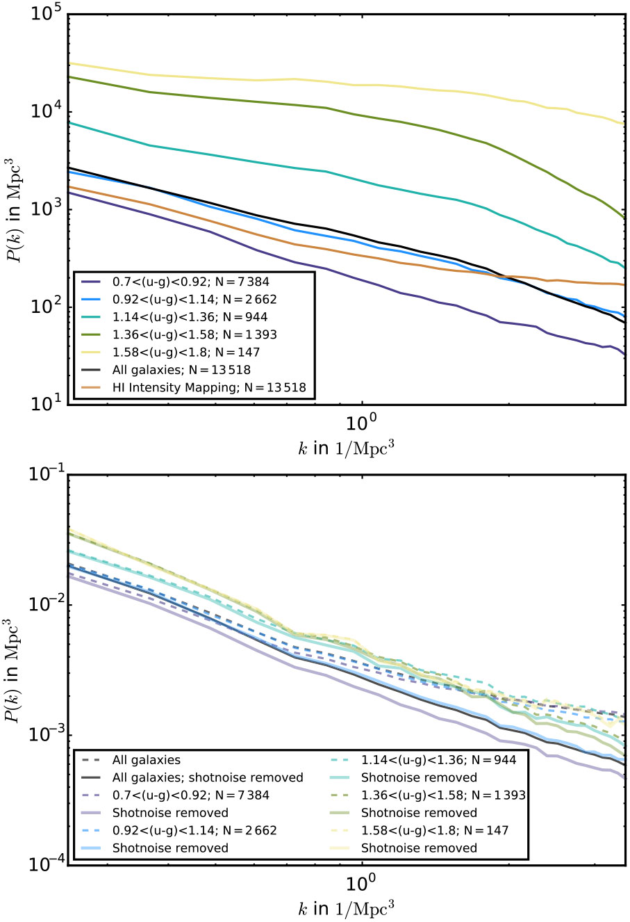
Figure 22. Upper panel: we use a box of the EAGLE hydro-dynamical simulation suite at  $z=0.5$ to derive the HI IM power spectrum (orange line) as well as several optical selected galaxy sample power spectra using the magnitudes in the SDSS u and g filters. The black line marks the power spectrum of all galaxies in the simulation volume. Lower panel: We cross-correlate the HI intensity maps with respective galaxy selections. The dashed lines mark the observed cross-power spectra. The solid lines have been shot noise corrected where the shot noise is proportional to the average HI mass in the optical galaxies.
SKA1-Mid and SKA1-Low will both be equipped to perform HI IM observations spanning  $0<z<6$. The resulting HI power spectrum measurements will allow the determination of the scale dependence of the HI bias, as well as the absolute amplitude of the HI bias when employing outside constraints for the HI energy density, $\Omega_{\rm HI}$. The cross-correlations of these observations with galaxy surveys performed by Euclid or LSST will provide additional insights into the coupling of galaxy and halo properties to the HI distribution.
The DM problems on galaxy scales can be studied with the SKA precursors, with the help of suitable samples of galaxies and long integration times to attain the necessary sensitivity to detect the HI as far out as possible. The accompanying multi-wavelength optical studies are also reaching a great sophistication, so that they hopefully set stringent constraints to the stellar mass-to-light ratios of galactic discs.
5.2.2. Thermal characteristics of DM
Determining the magnitude of the DM thermal velocities will give us clues to unveiling the nature of DM. We already know that DM cannot be hot, that is, it cannot be mostly made up of particles with large thermal velocities such as neutrinos, since this would change the structure formation paradigm from bottom-up to top-down. On the other hand, the possibility of DM having relatively small thermal velocities (i.e., WDM) is not in contradiction with cosmological observations. Currently, the tightest constraints come from observations of the Lyman- $\alpha$ forest (Iršič et al. 2017) with $m_{\rm WDM}>5.3$ keV at $2\sigma$ confidence, but a large parameter space remains unexplored and could in principle be investigated. The SKA can further constrain these WDM properties by measuring the global 21-cm evolution and power spectra in different frequency bands. The following sections summarise the effect of such thermal properties and the prospects for measurement.
5.2.3. WDM and the HI power spectrum
The shape and amplitude of the 21-cm power spectrum at different redshifts are sensitive to the abundance, clustering and HI mass function of DM halos. It is expected therefore that the significant impact WDM has on the properties of low-mass halos will result in an observable signature. The impact of WDM on halo properties has been studied in some detail, and analytic formalisms such as the halo model have been extended to include it (Dunstan et al. Reference Dunstan, Abazajian, Polisensky and Ricotti2011). Carucci et al. (Reference Carucci, Villaescusa-Navarro, Viel and Lapi2015) prepared forecasts using the results of hydrodynamic simulations with CDM and WDM and pointed out that 5 000 h of interferometer IM observations by SKA1-Low can be used to rule out a WDM model with an effective particle mass,  $m_{X}$, of 4 keV at $3\sigma$. These are competitive constraints that can complement bounds from independent probes such as those from the Lyman- $\alpha$ forest (Iršič et al. 2017).
To show the evolution of the power spectrum at different scales, Figure 23 plots the brightness temperature power spectrum as a function of redshift,  ${(\delta \bar{T}_b)^2\Delta_{21}^2}$, for the modes $k=0.08$ Mpc–1 and $k=0.18$ Mpc–1. One can see a three-peak structure that (moving from right to left) is due to inhomogeneities in the coupling coefficient for scattering of Lyman- $\alpha$ photons, $x_{\alpha}$, kinetic gas temperature, $T_{\rm K}$, and the neutral fraction of hydrogen, $x_{\text{HI}}$. At their peak, these inhomogeneities could enhance the power at $k=0.08,0.18$ Mpc–1 for the WDM model by up to a factor of $2.4, 2.0\,$ for $m_{\rm X}=2\,$keV and $1.3,1.1$ for $m_{\text{X}}=4$ keV model.
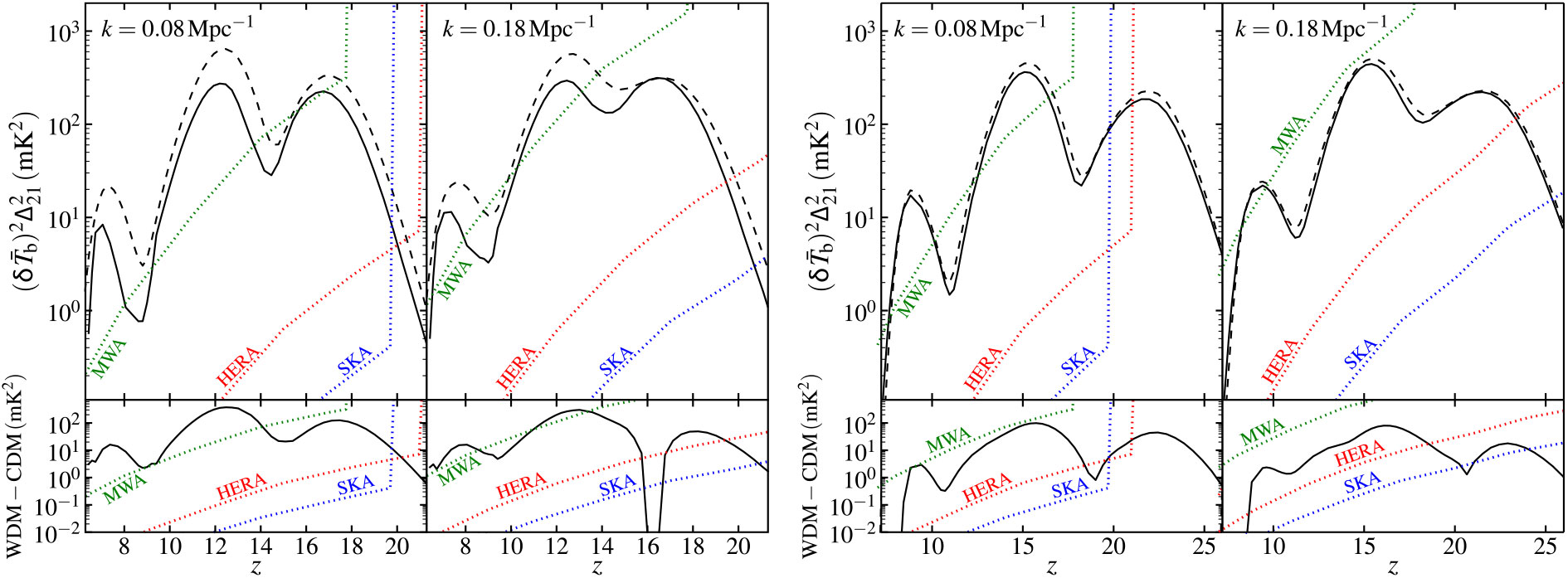
Figure 23. Evolution of the power spectrum of the brightness temperature for WDM with (left panel)  $m_{\text{X}}=2 \, \text{keV}$ and (right panel) $m_{\text{X}}=4 \, \text{keV}$. The top panels show power spectra at $k=0.08,~0.18~\text{Mpc}^{-1}$ for the WDM (dashed) and the CDM model (solid). The bottom panel is the subtraction of CDM power spectrum from the WDM power spectrum, showing the difference. The dotted curves show the $1\sigma$ thermal noise power spectrum forecasts computed by Mesinger et al. (Reference Mesinger, Ewall-Wice and Hewitt2014) and Sitwell et al. (Reference Sitwell, Mesinger, Ma and Sigurdson2014) with 2 000 h observational time. The green, red and blue lines are for MWA, HERA and SKA-Low respectively. Figure taken from Sitwell et al. (Reference Sitwell, Mesinger, Ma and Sigurdson2014).
The current interferometric radio surveys such as MWA, HERA, and SKA-Low may provide the sensitivity and noise level that are able to detect this boost of power spectrum by WDM. To forecast the capability of these new surveys to place constraints on WDM model, we plot the forecasts of  $1\sigma$ thermal noise of the power spectrum computed by Mesinger et al. (Reference Mesinger, Ewall-Wice and Hewitt2014) and Sitwell et al. (Reference Sitwell, Mesinger, Ma and Sigurdson2014) for 2 000 h of observational time for MWA, HERA, and SKA-Low in Figure 23. One can see that, although MWA’s capability is marginally able to detect the boosted power of $m_{\text{X}}=2\,$keV model at reionisation and X-ray heating peak locations, SKA-Low should provide a strong constraint on the excess power on these scales over the range of redshift $10<z<25$.
5.2.4. Determining thermal properties from the EoR
FF emission from an ionised medium can produce a potentially remarkable diffuse signal, particularly at frequencies lower than  $\sim\! 10$ GHz. The baryonic matter variance can be calculated by integrating the power spectrum of matter density perturbations over an appropriate range of wavenumbers:
 $$
\begin{equation}
\sigma^{2} (z) = \frac{1}{2\pi^{2}} \int P(k, z) k^{2 }dk .
\label{eqn26}
\end{equation}
$$
$$
\begin{equation}
\sigma^{2} (z) = \frac{1}{2\pi^{2}} \int P(k, z) k^{2 }dk .
\label{eqn26}
\end{equation}
$$ In a given cosmological model, the cosmological parameters determine the level of matter density contrast. While the structure distribution does not depend significantly on the DM model at large scales (Gao & Theuns Reference Gao and Theuns2007), the small scales and, consequently, the amplitude of the clumping factor,  $1+\sigma^2 (z)$, are particularly sensitive to the thermal properties of DM particles.
In CDM standard models, cold and essentially collisionless particles had a negligible velocity dispersion in the cosmic epochs relevant for structure formation, and the corresponding power spectrum is then essentially undamped up to very high wavenumbers. Contrariwise, in WDM models, the intrinsic thermal velocity dispersions related to the particle distribution properties could imply a substantial free-streaming process, affecting clustering properties and suppressing power spectrum above certain wavenumbers, dependent on particle thermal history and mass. Traditional cold and hot DM particle masses are, respectively, in the range of  $\sim\! 10 - 10^{2}$ GeV and $\sim$ few eV, while masses of about $1-10$ keV are typically considered for WDM particle candidates (Boyanovsky et al. Reference Boyanovsky, de Vega and Sanchez2008), in form of, for example, gravitinos or sterile neutrinos.
The evolution of the power spectrum can be described in terms of transfer function, and for WDM models it is approximately given by that of the corresponding CDM model but with with a cut-off  $k_\mathrm{max}$ at high wavenumbers, that is, at scales smaller than the scale of free streaming of the WDM particle. Values of $k_\mathrm{max}$ in the range 20– $10^3$ are usually considered. Thus, together with the amplitude of initial perturbations, $k_\mathrm{max}$ mainly determines the values the clumping factor at the relevant redshifts. In turn, the damping of inhomogeneities in $\Lambda$WDM models at small scales delays the growth of structures (Viel et al. Reference Viel, Williams, Shu and Menard2005), influencing the early stages of star formation history.
Ultimately, the non-negligible IGM density contrast, related to DM particle properties, implies an amplification factor of  $[\simeq 1 + \sigma^{2} (z)]$ of the diffuse FF emission triggered by a specific reionisation mechanism (Trombetti & Burigana Reference Trombetti and Burigana2014). Therefore, other than contributing to the deep understanding of the astrophysical reionisation process, the detailed analysis of the FF diffuse signal represents a way to study DM properties exploiting their influence on the power spectrum at high wavenumbers.
5.3. DM searches
The nature of DM will remain a mystery without the clear and unequivocal detection of its particle physics natureFootnote k. A surprisingly common prediction of many particle physics models is that DM is not completely dark. It can either couple to standard model particles with a very weak interaction or it can self-annihilate or decay, and via cascading processes eventually end up as standard model particles such as neutrinos, photons, positrons, and other antimatter elements (Bertone et al. Reference Bertone, Hooper and Silk2005).
Such particles may be observed through different channels. Neutrinos and photons, usually in the form of  $\gamma$-rays, have zero electromagnetic charge and consequently maintain their original trajectory. Conversely, charged particles are effectively isotropised by their tangled propagation in galactic magnetic fields. The acceleration of the charged particle products in the magnetic fields do, however, provide an additional detection channel via the emission of secondary radiation such as bremsstrahlung, Compton, or synchrotron radiation. The latter can reach frequencies from MHz to a few hundred GHz and needs to be isolated from overwhelming and complex astrophysical backgrounds that mask the expected DM signal both morphologically and in spectral features. The DM signals often possess features that differentiate them from the backgrounds (typically, a non-power-law spectrum and a cut-off at an energy related to the DM mass). This is not observed in the data (e.g., from Fermi, HESS, and MAGIC) and therefore relevant bounds on DM properties (particle mass, annihilation, or decay rate) are the typical outcome (e.g., Gaskins Reference Gaskins2016; Conrad & Reimer Reference Conrad and Reimer2017, and references therein).
The most studied option is the so-called WIMP, elementary particles with a mass from a few GeV to several TeV, endowed with weak or sub-weak type interactions. In particular,  $\gamma$-ray observations are considered a promising avenue to probe WIMP scenarios (Bringmann & Weniger Reference Bringmann and Weniger2012), but $\gamma$-rays alone cannot usually be disentangled from the astrophysical sources, and radio astronomy can play a crucial role in background determination. Although DM targets (clusters, galaxies, galaxy satellites, or subhalos) appear to be invisible individually, their cumulative emission might be detectable with advanced techniques. We will discuss possible general signals in Section 5.3.1 and more specific cases in Sections 5.3.2, 5.3.4, and 5.3.5. But as we will discuss in Sections 5.3.3 and 5.3.6, other options should also be considered.
5.3.1. Photon fluxes from WIMP-like DM
Positrons and electrons propagating in magnetic fields will lose energy (mainly) due to synchrotron radiation and inverse Compton scattering (Sarazin Reference Sarazin1999). Other ways to lose energy, such as Coulombian interactions or bremsstrahlung are subdominant. For the energies and magnetic fields relevant for DM positrons in the Milky Way, the resulting radiation has frequencies from MHz to a few hundred GHz. For high-energy positrons and electrons propagating in a galactic environment, the density per unit energy ( $\psi$ in units of cm-3 GeV-1) is well described as a purely diffusive equation (Delahaye et al. Reference Delahaye, Lineros, Donato, Fornengo and Salati2008):
 $$
\begin{eqnarray}
-K_{0}\epsilon ^{\delta}\nabla^{2}\psi-\frac{\partial}{\partial E}(b(E)\psi)=Q(\vec x,E),
\label{eqn27}
\end{eqnarray}
$$
$$
\begin{eqnarray}
-K_{0}\epsilon ^{\delta}\nabla^{2}\psi-\frac{\partial}{\partial E}(b(E)\psi)=Q(\vec x,E),
\label{eqn27}
\end{eqnarray}
$$ in which the parameters  $K_{0}$ and $\delta$ model the diffusion of the positrons in the galactic magnetic field, b(E) describes the loss of energy, and $\epsilon=E/1\,{\rm GeV}$.
The source term  $Q(\vec x,E)$ contains the information on the source that injects positrons into the environment. If the only primary source of positrons is the annihilation of WIMP particles with mass M, the source term becomes
 $$
\begin{eqnarray}
Q(\vec{x},E)=\frac{1}{2}\left\langle \sigma v\right\rangle\left(\frac{\rho(\vec x)}{M_{\text{}}}\right)^2\sum_{i}\beta_{j}\frac{{\rm d}N_e^j}{{\rm d}
E},
\label{eqn28}
\end{eqnarray}
$$
$$
\begin{eqnarray}
Q(\vec{x},E)=\frac{1}{2}\left\langle \sigma v\right\rangle\left(\frac{\rho(\vec x)}{M_{\text{}}}\right)^2\sum_{i}\beta_{j}\frac{{\rm d}N_e^j}{{\rm d}
E},
\label{eqn28}
\end{eqnarray}
$$ where  $\beta_{j}$ is the branching ratio of the different annihilation channels. The thermally averaged annihilation cross section, $\langle\sigma v\rangle$, is mainly described by the theory explaining the WIMP physics, whereas the number of positrons and electrons produced in each decay channel per energy interval, $\text{d}\,N_\gamma^i/\text{d}\,E_{\gamma}$ involves decays and/or hadronisation of unstable products (e.g., quarks and gauge bosons) involving non-perturbative effects related to quantum chromodynamics (QCD), which can be obtained from numerical software packages such as DarkSUSYFootnote l or micrOMEGAsFootnote m based on PYTHIA Monte Carlo event generatorFootnote n.
The power of emission is related to the positron kinetic energy by the synchrotron power
 $$
\begin{eqnarray}
P_\mathrm{syn}=\frac{1}{4\pi \epsilon_{0}} \frac{\sqrt{3}e^{3} B}{m_{e} c} y \int^{\infty}_{y} {\rm d}\xi\, K_{5/3}(\xi) \left(\frac{\nu}{\nu_{c}}\right),
\label{eqn29}
\end{eqnarray}
$$
$$
\begin{eqnarray}
P_\mathrm{syn}=\frac{1}{4\pi \epsilon_{0}} \frac{\sqrt{3}e^{3} B}{m_{e} c} y \int^{\infty}_{y} {\rm d}\xi\, K_{5/3}(\xi) \left(\frac{\nu}{\nu_{c}}\right),
\label{eqn29}
\end{eqnarray}
$$where
 $$
\begin{eqnarray}
\nu_{c} =\frac{3eE^{2} B}{4\pi m_{e}^{3} c^{4}}
\label{eqn30}
\end{eqnarray}
$$
$$
\begin{eqnarray}
\nu_{c} =\frac{3eE^{2} B}{4\pi m_{e}^{3} c^{4}}
\label{eqn30}
\end{eqnarray}
$$ is defined as the critical frequency of the emission. In the above equations, B is the galactic magnetic field,  $m_{e}$ the mass of the electron, E the kinetic energy of the electron/positrons, c the speed of light, and $K_{5/3}(\xi)$ is the modified Bessel function of the second kind.
Taking into consideration every positron and electron with a specific energy as a synchrotron emitter, it is necessary to sum all the possible contributions over the line of sight as follows:
 $$
\begin{eqnarray}
F(\nu)=\left(\frac{2}{4 \pi}\right) \int_\mathrm{l.o.s} {\rm d}l \int^{M}_{m_{e}}{\rm d}
E'\, P_{\rm syn}(\nu,E') \psi (\vec{x},E')\,.
\label{eqn31}
\end{eqnarray}
$$
$$
\begin{eqnarray}
F(\nu)=\left(\frac{2}{4 \pi}\right) \int_\mathrm{l.o.s} {\rm d}l \int^{M}_{m_{e}}{\rm d}
E'\, P_{\rm syn}(\nu,E') \psi (\vec{x},E')\,.
\label{eqn31}
\end{eqnarray}
$$  $F(\nu)$ corresponds to the so-called density of radiation (which can be measured in janskys) and $\psi (\vec{x},E')$ is the number density of electrons/positrons previously calculated through the diffusion equation in Equation (29). Focusing on the Milky Way, a diffuse contribution in radio frequencies could be expected due to the disposition of DM in halos.
5.3.2. Searches for diffuse emission in the darkest sources
As described in Section 5.3.1, DM annihilations may cascade to non-thermal electrons and positrons, which in turn emit radio waves as synchrotron radiation in regions where an ambient magnetic field is present. Therefore, a generic prediction of WIMP models is diffuse radio emission from DM halos induced by non-gravitational interactions of DM. Its discovery would be a significant step towards the solution of the DM mystery. The improved sensitivity of the SKA and its precursors will allow us to reach the sensitivity required to detect the radio flux emitted by DM halos, especially at low redshifts, both in the investigation of the number counts of sources and in their statistics across the sky.
Intriguingly, a few years ago, the ARCADE-2 collaboration reported isotropic radio emission that is significantly brighter than the expected contributions from known EG astrophysical sources (Seiffert et al. Reference Seiffert2011; Fornengo et al. Reference Fornengo, Lineros, Regis and Taoso2014) and is well fitted by WIMP-induced emission (Fornengo et al. Reference Fornengo, Lineros, Regis and Taoso2011). If the cosmological signal from DM is at such level, then the contribution from particle DM in the data from the Evolutionary Map of the Universe (EMU; Norris et al. Reference Norris2011) survey on the Australian Square Kilometre Array Pathfinder (ASKAP; Johnston & Wall 2008) should be significant.
Figure 24 shows the number of sources as a function of redshift in two brightness ranges for the DM component (for model A of Fornengo et al. Reference Fornengo, Lineros, Regis and Taoso2011, which fits the ARCADE excess), compared to more mundane astrophysical sources that explain the source counts observed so far. The emission from DM is mainly provided by faint sources at low redshift, and the median size of the source is large ( $\gtrsim$ arcmin). This implies that previous analyses of counts or angular correlation were not sensitive to a WIMP-induced signal. A relevant exception is Vernstrom et al. (Reference Vernstrom, Norris, Scott and Wall2015), who interestingly reported a possible deviation associated with faint extended sources. Figure 24 shows that while the DM contribution is subdominant in the range probed by NRAO Very Large Array Sky Survey (NVSS, above mJy), it can become relevant for fluxes within the sensitivity reach of the SKA and its precursors.
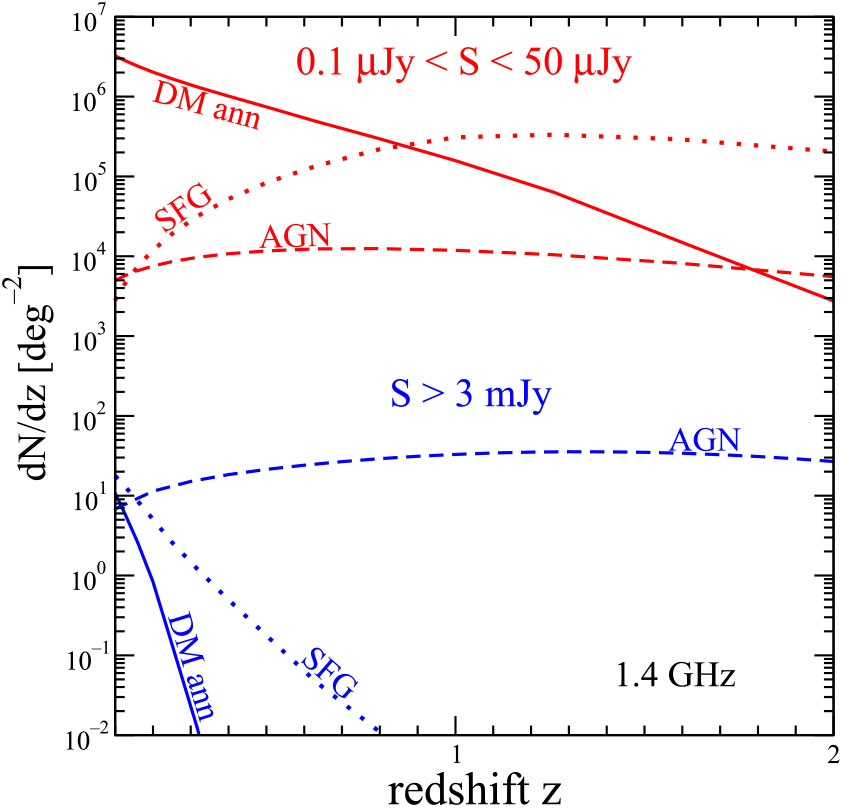
Figure 24. Redshift distribution of sources for bright ( $S> 3$ mJy, lower in blue) and faint ( $0.1\, \mu\rm{Jy} < S < 50\, \mu\rm{Jy}$, upper in red) samples, showing that DM annihilation will be visible in the faint source number count but not in the bright source number count. Benchmark models for astrophysical and DM radio sources are taken from Fornengo et al. (Reference Fornengo, Lineros, Regis and Taoso2012a).
The analysis of number count fluctuations in SKA data and the angular auto- and cross-correlation of the SKA density field are thus promising techniques to test the DM interpretation of the ARCADE excess and, more generally, to constrain the WIMP parameter space (Fornengo et al. Reference Fornengo, Lineros, Regis and Taoso2012a).
5.3.3. Branons as WIMP candidates
Massive brane fluctuations (branons) provide an example of a DM candidate that is detectable or constrainable with the SKA. They arise in brane-world models with low tension (Cembranos et al. Reference Cembranos, Dobado and Maroto2003b; Cembranos et al. Reference Cembranos, Dobado and Maroto2003a; Kugo & Yoshioka Reference Kugo and Yoshioka2001).
Massive branons are pseudo-scalar fields that can be understood as the pseudo-Goldstone bosons corresponding to the spontaneous breaking of translational invariance in the bulk space. The broken symmetry is precisely produced by the presence of the brane (Sundrum Reference Sundrum1999; Bando et al. Reference Bando, Kugo, Noguchi and Yoshioka1999; Dobado & Maroto Reference Dobado and Maroto2001). Branons are prevented from decaying into standard model particles by parity invariance on the brane, but can annihilate into standard model particles, although the coupling is suppressed by the brane tension scale. The branons are mass degenerate, and consequently the annihilation fluxes only depend upon two parameters of the effective theory describing the low-energy dynamics of flexible brane-worlds, namely the brane tension scale and the branon mass, M (Cembranos et al. Reference Cembranos, Dobado and Maroto2001b,a, Reference Cembranos, Dobado and Maroto2004; Alcaraz et al. Reference Alcaraz, Cembranos, Dobado and Maroto2003). Bounds and constraints on the model parameters from cosmology and tree-level processes in colliders are shown in Figure 25 (Kugo & Yoshioka Reference Kugo and Yoshioka2001; Cembranos et al. Reference Cembranos, Dobado and Maroto2003a; Maroto Reference Maroto2004a, b). Further astrophysical and cosmological bounds serve to parametrise the tension in terms of the branon mass, rendering the dynamics dependent on the mass alone (Kugo & Yoshioka Reference Kugo and Yoshioka2001; Cembranos et al. Reference Cembranos, Dobado and Maroto2003a; Maroto Reference Maroto2004a, b).
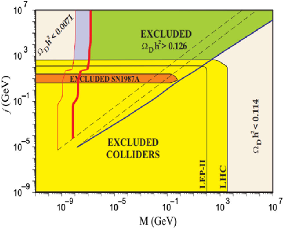
Figure 25. Combined exclusion plot for a branon model with a single disformal scalar from total and hot DM (taken from Cembranos & Maroto Reference Cembranos and Maroto2016) including constraints from LEP-II (Alcaraz et al. Reference Alcaraz, Cembranos, Dobado and Maroto2003; Achard et al. Reference Achard2004) and LHC (Cembranos et al. Reference Cembranos, Dobado and Maroto2004, Reference Cembranos, Diaz-Cruz and Prado2011; Landsberg Reference Landsberg2015; Khachatryan et al. Reference Khachatryan2016) single photon event, and supernova cooling (Cembranos et al. Reference Cembranos, Dobado and Maroto2003c). The two solid (red) lines on the right are associated with the hot DM; the thicker line corresponds to the total DM range  $\Omega_{D} h^{2}= 0.126-0.114$ (Ade et al. Reference Ade2016) and the thin line is the hot DM limit $\Omega_{D} h^{2}<0.126-0.114$. The solid (blue) line along the diagonal corresponds to CDM behaviour, and the dashed lines corresponds to $M/T_\mathrm{freeze-out} = 3$ for hot (upper curve) and cold (lower curve) DM.
For branons, the thermally averaged annihilation cross sections depend solely upon the spin and the mass of the branon (Cembranos et al. Reference Cembranos, Dobado and Maroto2003c, 2006). In the case of heavy branons  $M \gg m_{W,\,Z}$, the main contribution to the indirect photon flux comes from branon annihilation into bosons, $W^+W^-$ and ZZ. The contribution from heavy fermions, that is the annihilation into top-antitop, can be shown to be subdominant. On the contrary, whenever $M \ll m_{W,\,Z}$, the annihilation into W or Z bosons is kinematically forbidden so that the remaining channels must be considered, mainly annihilation into the heaviest possible quarks (Cembranos et al. Reference Cembranos, de la Cruz-Dombriz, Gammaldi and Maroto2012).
Figure 26 shows the expected synchrotron flux densities from DM annihilations in the GC for various annihilation channels (upper and middle panels) for a generic WIMP or different branon masses (lower panel). Consequently, the SKA would have the potential to disentangle different model-independent DM masses and the preferred annihilation channel(s) (upper and middle panels) as well as different branon candidates (lower panel) by combining different frequency ranges. For example, one can see the SKA1-Mid band-1 (0.35–1.05 GHz) and SKA1-Mid band-4 (2.80–5.18 GHz), and the sensitivity to both the DM annihilation channels and also DM masses (see Colafrancesco et al. Reference Colafrancesco, Regis, Marchegiani, Beck, Beck, Zechlin, Lobanov and Horns2015). In addition, since the SKA minimum detectable density flux would lie on the  $\sim\!\mu\text{Jy}$ range (Cembranos et al. Reference Cembranos, de la Cruz-Dombriz, Gammaldi and Mendez-Isla2019), such inferences would be feasible for the depicted fluxes.
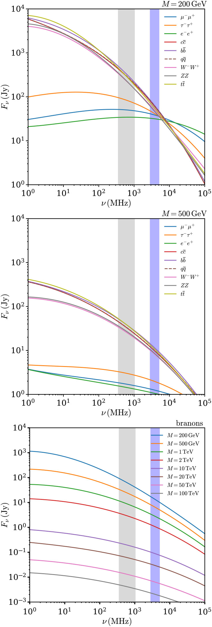
Figure 26. Synchrotron density fluxes from the GC ( $l=0^{ o},b=0^{ o}$ in galactic coordinates) for different channels of branons spontaneous annihilations. Channel $q\overline{q}$ corresponds to the annihilation via $u\overline{u}$, $d\overline{d}$ and $s\overline{s}$. The first panel represents a DM mass of $\text{M}=200$ GeV and the second one is for a mass of $\text{M}=1\,000$ GeV. The diffusion considered was $\text{K}_{0}=0.00595\,\text{kpc}^{2}/\text{MYr}$, $\delta=0.55$ and $\text{L}_{\text{z}}= 1$ kpc and the DM density profile used was the isothermal. The considered magnetic field is $6 \mu \text{G}$. As we can see, the synchrotron signal decreases more drastically in the case of the $W^{+}W^{-}$, $Z^{+}Z^{-}$ bosons and $q\overline{q}$, $t\overline{t}$, $b\overline{b}$ and $c\overline{c}$ quarks than the signal of the leptonic channels. The signal increases at low frequencies showing the suitable ranges to detect the signature. No boost factors are considered in this figure. In the lower panel, the signature decrease as a function of mass has been exemplified for a model with one extra dimension with a tension of $f=8.25~ {\rm M}^{0.75}$ (Cembranos et al. Reference Cembranos, Dobado and Maroto2003a, c)
In Figure 26, we show the predicted fluxes for branon masses in the range of 200 GeV to 100 TeV, so that the principal channels of annihilation are via W and Z bosons and the top quark. Qualitatively, we observe that the radio emission shape depends on the annihilation channel, potentially providing information about the nature of the branon. In addition, we observe that for branons (with a brane tension that depends on the mass), the expected signature decreases with the mass. That means that detectable signatures can be associated with low masses of this extra-dimensional particle. Furthermore, this methodology of obtaining the flux density will allow us to discard regions of parameter space in the case where we observe a smaller signal than predicted by experimental results.
Finally, a monochromatic  $\gamma$-ray line is expected at the energy equal to the branon mass as a consequence of direct annihilation into photons. This annihilation takes place in the d-wave channel. Consequently, it is highly suppressed and is not detectable with current instruments (e.g., Fermi; Cembranos et al. Reference Cembranos, de la Cruz-Dombriz, Gammaldi and Maroto2012). However, masses above 150 GeV can potentially be detected with the increased sensitivity of the Cherenkov Telescope Array, in which case cross-correlation with a synchrotron signal from the SKA becomes a crucial test.
5.3.4. Cross-correlation of SKA1 HI galaxies and γ -rays
Faint sources of emission from DM might not be detectable on their own, but they contribute a cumulative component. This method builds on a recent proposal to use cross-correlations between a gravitational tracer of DM (cosmic shear or galaxy clustering as proxies for the DM distribution in the Universe) and any DM-sourced electromagnetic signals (Camera et al. 2013 b; Fornengo & Regis Reference Fornengo and Regis2014). In addition, it has the potential to bring redshift information to the electromagnetic signal that is otherwise unavailable, exploiting the different behaviour of DM emission peaking at low redshift and the unresolved astrophysical production of the same observables more pronounced towards intermediate redshift (e.g., Camera et al. Reference Camera, Fornasa, Fornengo and Regis2013b, Reference Camera, Fornasa, Fornengo and Regis2015d; Fornengo et al. Reference Fornengo, Perotto, Regis and Camera2015; Xia et al. Reference Xia, Cuoco, Branchini and Viel2015; Branchini et al. Reference Branchini, Camera, Cuoco, Fornengo, Regis, Viel and Xia2017; Tröster et al. Reference Tröster2017). Specifically, we discuss here the impact of the catalogue of HI galaxies that will be obtained by the SKA on the cross-correlation with Fermi Large Area Telescope (LAT)  $\gamma$-ray maps.
Currently, the vast majority of the  $\gamma$-ray sky is unresolved and only a few thousand $\gamma$-ray sources are known. The two frequency regimes where, on large scales, non-thermal emission mechanisms are expected to exceed greatly any other process are the low-frequency radio band and the $\gamma$-ray range. Radio data are thus expected to correlate with the $\gamma$-ray sky and can be exploited to filter out information on the composition of the $\gamma$-ray background contained in unresolved $\gamma$-ray data.
Indeed, a cross-correlation between the unresolved  $\gamma$-ray background seen by the Fermi-LAT telescope and the distribution of sources detected in continuum in the NVSS (Condon et al. Reference Condon, Cotton, Greisen, Yin, Perley, Taylor and Broderick1998) catalogue has been recently detected (Xia et al. Reference Xia, Cuoco, Branchini and Viel2015). The angular power spectrum data are shown in Figure 27 together with a reference model (Cuoco et al. Reference Cuoco, Xia, Regis, Branchini, Fornengo and Viel2015). Combining this measurement with other catalogues, relevant constraints on the composition of the $\gamma$-ray background can be derived (Xia et al. Reference Xia, Cuoco, Branchini and Viel2015; Cuoco et al. Reference Cuoco, Xia, Regis, Branchini, Fornengo and Viel2015; Ammazzalorso et al. Reference Ammazzalorso2019). The improvement in sensitivity offered by ASKAP and the SKA is dramatic, as shown in the example of the EMU survey (grey area) in Figure 27. SKA and precursor data will therefore allow us to discriminate between different explanations for the composition of the $\gamma$-ray background.
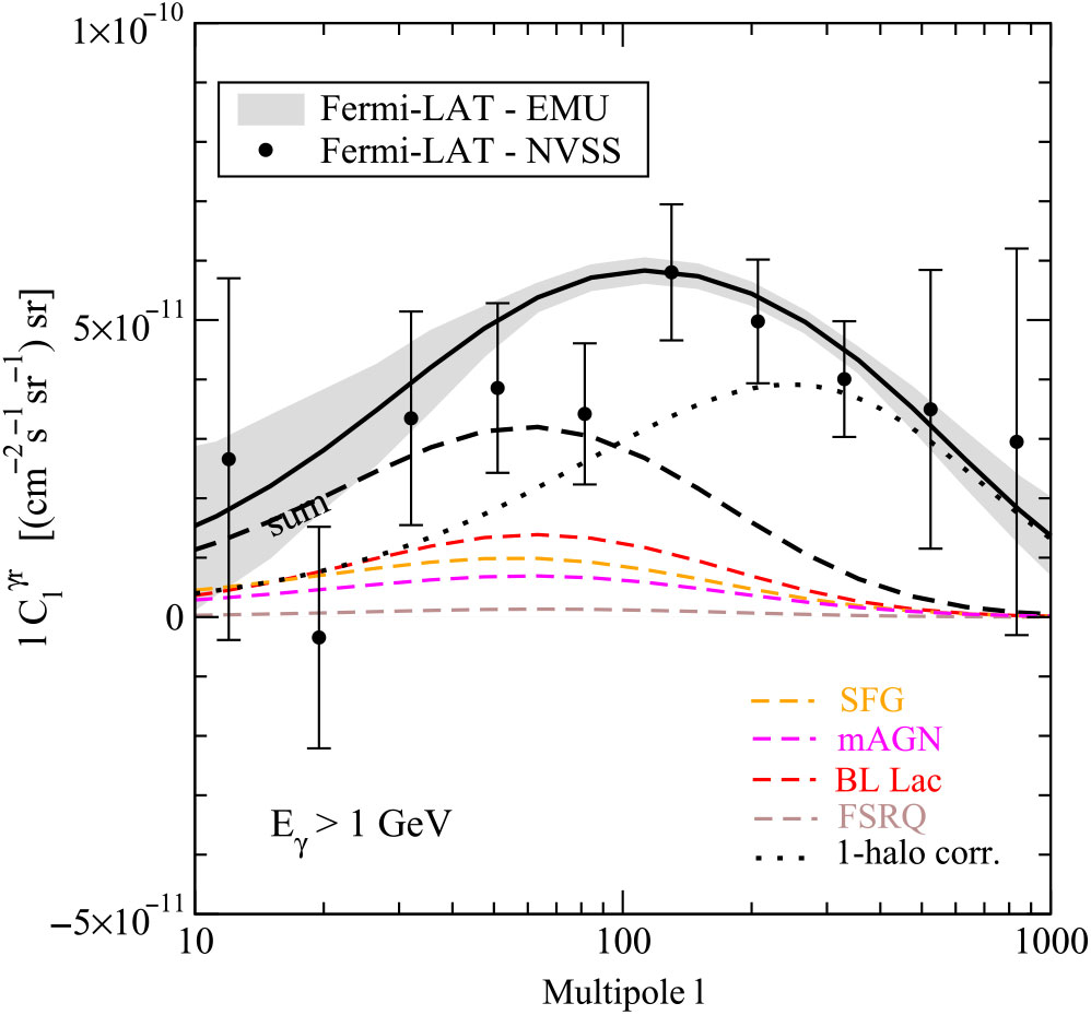
Figure 27. Angular power spectrum of cross-correlation between the unresolved  $\gamma$-ray background and the distribution of radio sources. Data points refer to the measurement performed using Fermi-LAT and NVSS data, the solid curve shows a reference model, and the grey area reports the expected sensitivity for the cross-correlation between EMU and Fermi-LAT data. For details concerning data and models see, Xia et al. (Reference Xia, Cuoco, Branchini and Viel2015) and Cuoco et al. (Reference Cuoco, Xia, Regis, Branchini, Fornengo and Viel2015), respectively.
Following on from these seminal observational results and the techniques and forecasts first proposed by Camera et al. (Reference Camera, Fornasa, Fornengo and Regis2013b, Reference Camera, Fornasa, Fornengo and Regis2015d) and Fornengo & Regis (Reference Fornengo and Regis2014), we present some preliminary results on the cross-correlation of SKA1 HI galaxies and the  $\gamma$-ray sky from Fermi. Note that, contrary to NVSS and EMU, in this case we use HI galaxies for which spectroscopic redshifts will be available. This will allow us to exploit fully the tomographic-spectral approach outlined in Camera et al. (Reference Camera, Fornasa, Fornengo and Regis2015d). Moreover, there is major added value in the use of SKA1 HI galaxies, their redshift distribution peaking at low redshift and having an extremely low shot noise (see Figure 4 of Yahya et al. Reference Yahya, Bull, Santos, Silva, Maartens, Okouma and Bassett2015). This is the very regime where the non-gravitational DM signal is the strongest. The emission associated with WIMP decay is proportional to the DM density, and consequently stronger at low redshift because the produced radiation is diluted by the expansion of the Universe more rapidly than its source. The WIMP annihilation signal, proportional to the density squared, also peaks at low redshift since the density contrast associated with cosmic structures grows non-linearly at late times.
Specifically, we adopt an SKA1 HI galaxy survey with specifics given by Yahya et al. (Reference Yahya, Bull, Santos, Silva, Maartens, Okouma and Bassett2015) for the baseline configuration. We consider only galaxies in the redshift range  $0<z\le0.5$, which we further subdivide into 10 spectroscopic, narrow redshift bins. For the $\gamma$-ray angular power spectrum, we employ the fitting formulae found by Tröster et al. (Reference Tröster2017) for Pass-8 Fermi-LAT events gathered over 8 yr through to September 2016. This is a very conservative approach, as by the time the SKA1 HI galaxy catalogue will be available, Fermi-LAT will have produced a much larger amount of data.
Figure 28 preliminarily shows the precision with which we will be able to reconstruct the WIMP cross section and mass in the case of a DM candidate with  $m_{\rm DM}=100$ GeV and thermal cross section $3\times10^{-26}$ cm $^3$ s–1. The green contour (the same as in Figure 4 of Camera et al. Reference Camera, Fornasa, Fornengo and Regis2015d) refers to the cross-correlation of Fermi-LAT $\gamma$ rays and cosmic shear from DES, while the blue contour depicts the constraining power of an SKA1-Fermi joint analysis. The main take-home message here is the high complementarity of the two techniques, the combination of which (red ellipse) has the potential to tightly constrain both WIMP mass and cross section.
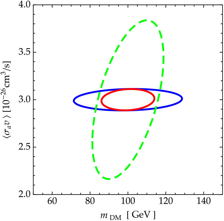
Figure 28. Joint 1 $\sigma$ marginal error contours on WIMP parameters for Fermi LAT $\gamma$-ray data cross-correlated with DES cosmic shear (green), SKA1 HI galaxies (blue) and their combination (red).
5.3.5. SKA1-Mid and MSPs
Given the large DM density in the inner Galaxy, any WIMP annihilation signal is expected to be particularly bright from that direction. Interestingly, a signal candidate has been found in  $\gamma$-ray data from the Fermi-LAT (Goodenough & Hooper Reference Goodenough and Hooper2009; Vitale & Morselli Reference Vitale and Morselli2009). The existence of an excess emission in the GeV energy range (
 $\sim\!100 \, \rm MeV - 10 \, \rm
GeV$), above conventional models for the diffuse
$\sim\!100 \, \rm MeV - 10 \, \rm
GeV$), above conventional models for the diffuse  $\gamma$-ray emission from the Galaxy, is now firmly established (Abazajian et al. Reference Abazajian, Canac, Horiuchi and Kaplinghat2014; Calore et al. Reference Calore, Cholis and Weniger2015; Ajello et al. Reference Ajello2016; Daylan et al. Reference Daylan, Finkbeiner, Hooper, Linden, Portillo, Rodd and Slatyer2016; Ackermann et al. Reference Ackermann2017). However, the signal may also have an astrophysical origin, for example, from the combined emission of thousands of MSPs in the galactic bulge (Wang Reference Wang2006; Abazajian Reference Abazajian2011), young pulsars (O’Leary et al. Reference O’Leary, Kistler, Kerr and Dexter2016), or stellar remnants from disrupted globular clusters (Brandt & Kocsis Reference Brandt and Kocsis2015).
We briefly summarise how the sensitivity of the SKA to detect the bulge population of MSPs can be estimated. Following Dewey et al. (Reference Dewey, Stokes, Segelstein, Taylor, Weisberg, Reynolds and Stinebring1984), the root mean square uncertainty of the flux density (in mJy) is given by
 $$
\begin{align}
S_{\nu, \rm rms} = \frac{T_{\rm sys}}{G \, \sqrt{t_{\rm obs} \, \Delta
\nu \, n_p}} \left(\frac{W_{\rm obs}}{P-W_{\rm obs}}
\right)^{1/2}\!\,,
\label{eqn32}
\end{align}
$$
$$
\begin{align}
S_{\nu, \rm rms} = \frac{T_{\rm sys}}{G \, \sqrt{t_{\rm obs} \, \Delta
\nu \, n_p}} \left(\frac{W_{\rm obs}}{P-W_{\rm obs}}
\right)^{1/2}\!\,,
\label{eqn32}
\end{align}
$$ where  $T_{\text{sys}}$ refers to the system temperature, G the instrument gain, $t_{\text{obs}}$ the observation time, $\Delta\nu$ the bandwidth, and $n_p=2$ the number of polarisations. Furthermore, P is the pulse period, and $W_{\text{obs}}$ the effective pulse width. We adopt the parameters corresponding to SKA1-Mid observations (Dewdney et al. Reference Dewdney, Turner, Millenaar, McCool, Lazio and Cornwell2013). More specifically, we adopt a central frequency of $1.67$ GHz, a 770 MHz bandwidth, a receiver temperature of 25 K, and an effective gain of 8.5 K Jy–1 for the considered sub-array (see Calore et al. Reference Calore, Di Mauro, Donato, Hessels and Weniger2016, for details). The beam full-width half-maximum is 0.77 arcmin, and we assume 3000 synthesised beams and 20 min of integration time per pointing.
We find that a dedicated search in the region ( $|\ell|<5^\circ$ and $3^\circ<|b|<7^\circ$) plus ( $|\ell|<3^\circ$ and $1^\circ<|b|<3^\circ$) plus ( $|\ell|,|b|<1^\circ$), which would take about 90 h, can detect 207 bulge and 112 foreground sources at $10\sigma$ significance or higher. This number is about seven times larger than the number of sources expected for a similar survey with MeerKAT. As shown in Figure 29, the SKA will be able to detect three times fainter sources than what is accessible by an equivalent MeerKAT survey, or by targeted observations with the GBT.
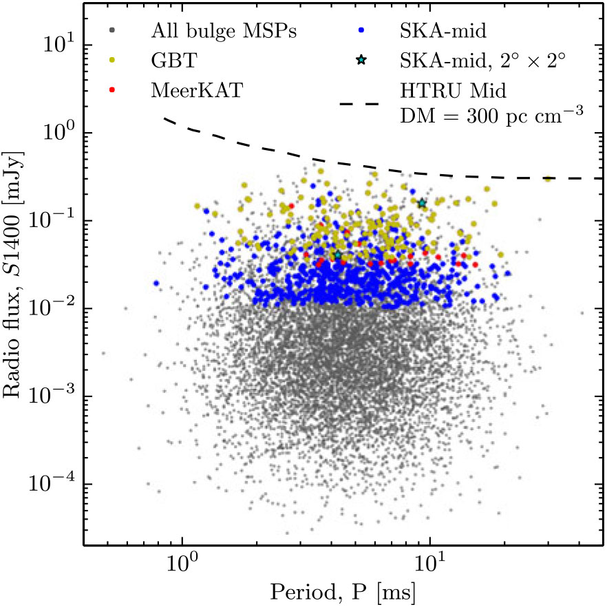
Figure 29. Distribution of the period vs. flux density of simulated bulge MSPs (grey dots). Sources detectable by the three observational scenarios described by Calore et al. (Reference Calore, Di Mauro, Donato, Hessels and Weniger2016) are represented by coloured dots. The improvement of SKA1-Mid with respect to the GBT and MeerKAT is represented by the blue points. ‘SKA-Mid  $2\times2$’ refers to sources detectable in the inner $2^\circ\times2^\circ$ about the GC. The dashed black line is the flux sensitivity of the Parkes High Time Resolution Universe mid-latitude survey (for DM $= 300$ pc cm–3). Figure adopted from Calore et al. (Reference Calore, Di Mauro, Donato, Hessels and Weniger2016).
The large number of detections will mark significant progress for our understanding of the MSP bulge population, and hence backgrounds for DM searches in the inner Galaxy. First, the large number of detections will allow us to determine the number of radio-bright bulge MSPs down to 10% precision, and to measure the distribution of sources and confirm that they indeed correspond to the morphology of the Fermi GeV excess. Second, the large number of measured ephemerides will be useful for searches for  $\gamma$-ray pulsations in the Fermi LAT data and likely allow us to significantly increase the part of the inner Galaxy $\gamma$-ray emission that can be directly attributed to MSPs. Third, anticipating a better determination of a potential correlation between $\gamma$-ray and radio emission, these results can lead to relatively clear predictions for the $\gamma$-ray emission from the galactic bulge that can then be subtracted from DM signal searches.
Finally, we stress that a non-detection of a significant number of bulge MSPs with the SKA would practically exclude the MSP hypothesis as explanation for the Fermi GeV excess, and strengthen the case for a DM signal, unless the radio emission of MSPs is a factor 10–100 weaker than what is suggested by globular clusters, while keeping the  $\gamma$-ray emission unchanged.
5.3.6. Extremely weakly interacting DM candidates
Looking for radio signals could be equally (if not more) important than searching for anomalous  $\gamma$-ray production. Radio signatures have already ruled out GeV DM particles with thermal interactions, have constrained DM models in general (e.g., Boehm et al. Reference Boehm, Ensslin and Silk2004; Crocker et al. Reference Crocker, Bell, Balazs and Jones2010; Boehm et al. Reference Boehm, Silk and Ensslin2010; Fornengo et al. Reference Fornengo, Lineros, Regis and Taoso2012b; Bringmann et al. Reference Bringmann, Vollmann and Weniger2014; Cirelli & Taoso Reference Cirelli and Taoso2016), and could further be used to probe the existence of extremely weakly interacting DM.
5.3.6.1. BH shadow
The DM density profile increases in the inner regions of galaxies, but the ‘spikiness’ of the profile is under debate. One hypothesis is that the DM density profile becomes as steep as  $\rho \propto r^{-7/3}$ near the central BH, referred to as a DM spike. The formation and survival of DM spikes is controversial (partly due to galaxy dynamics); however, one can test their existence if one further assumes that DM interacts (even very weakly) with standard model particles. Indeed, taking the specific case of heavy DM particles annihilating into standard model particles, it was shown that the presence of a DM spike in M87 leads to a copious production of synchrotron emission in the frequency range and spatial region that is currently being probed by the Event Horizon Telescope.Footnote o As the additional radiation from DM further enhances the photon ring around the BH shadow for any value of the self-annihilation cross section greater than $10^{-31}$ cm $^3$ s–1 (assuming a 10 GeV candidate), one should be able to confirm the presence of DM spikes even in scenarios of light p-wave annihilating DM candidates (Lacroix et al. Reference Lacroix, Karami, Broderick, Silk and Boehm2017).
5.3.6.2. Dark Ages
Alternative DM scenarios include particles with self and/or interactions with standard model particles in the early Universe. One consequence of these interactions is the damping of the primordial DM fluctuations, leading to a small-scale cut-off in the primordial power spectrum (see e.g., de Laix et al. Reference de Laix, Scherrer and Schaefer1995; Boehm et al. Reference Boehm, Fayet and Schaeffer2001, Reference Boehm, Riazuelo, Hansen and Schaeffer2002; Boehm & Schaeffer Reference Boehm and Schaeffer2005; Mangano et al. Reference Mangano, Melchiorri, Serra, Cooray and Kamionkowski2006). A late-time manifestation of these effects is the suppression of small-scale companions of the Milky Way as well as a smaller number of small structures in the Universe as a whole, which becomes even more prominent as one goes back in time (Boehm et al. Reference Boehm, Schewtschenko, Wilkinson, Baugh and Pascoli2014; Schewtschenko et al. Reference Schewtschenko, Wilkinson, Baugh, Boehm and Pascoli2015, Reference Schewtschenko, Baugh, Wilkinson, Boehm, Pascoli and Sawala2016; Cyr-Racine et al. Reference Cyr-Racine, Sigurdson, Zavala, Bringmann, Vogelsberger and Pfrommer2016; Vogelsberger et al. Reference Vogelsberger, Zavala, Cyr-Racine, Pfrommer, Bringmann and Sigurdson2016; Moline et al. Reference Moline, Schewtschenko, Palomares-Ruiz, Boehm and Baugh2016). By probing the Dark Ages, the SKA will be able to measure the primordial power spectrum at high redshift and probe a potential suppression of power due to the nature of the DM.
5.3.6.3. Axions
An alternative to the WIMP DM model is that some or all of the DM is comprised of QCD axions.
Axion-two photon coupling in the astrophysical environment may result in an observable DM signature, with the strength and shape of the axion signature strongly dependent on the relative properties of the magnetic field. Assuming that the axion comprises a substantial component of the CDM density, conversion in a static magnetic field will produce a line profile with central frequency principally derived from the mass of the axion, that is in the range  $0.2-200$ GHz. The width and polarisation of the signal is then dependent on the velocity distribution of the axion, the relative movement of the Earth and the source, and the polarisation of the magnetic field itself (see also Section 5.4.4 on the SKA’s ability to trace magnetic fields). In fact, the polarisation and strength of the axion signal should trace the spatial profile of the magnetic field. This is of particular use in extracting the axion signature from other foreground signals, since the polarisation should be perpendicular to synchrotron radiation.
With such distinguishing features, new technologies offer the opportunity for astrophysical observations to make a significant contribution to axion search efforts. Laboratory experiments searching for the axion have received significant investment in recent years but remain sensitive only to the most optimistic axion model and operate over small areas in frequency space. SKA2 in particular offers a significant improvement in the axion coupling strength that can be probed and in the breadth of frequency space that can be observed. To demonstrate the potential power of the SKA and its precursors, Figure 30 (taken from Kelley & Quinn Reference Kelley and Quinn2017) shows the axion-two photon coupling strength that could be probed with observations of the interstellar medium, the parallel lines from the bottom-left to top-right showing the coupling strength expected from the Kim-Shifman-Vainshtein-Zakharov (KSVZ) and Dine-Fischler-Srednicki-Zhitnitsky (DFSZ) models (Kim Reference Kim1979; Shifman et al. Reference Shifman, Vainshtein and Zakharov1980; Dine et al. Reference Dine, Fischler and Srednicki1981). Further constraint of this parameter space with the SKA, or indeed detection of the axion itself, would represent an important step forward in both particle physics and cosmology.
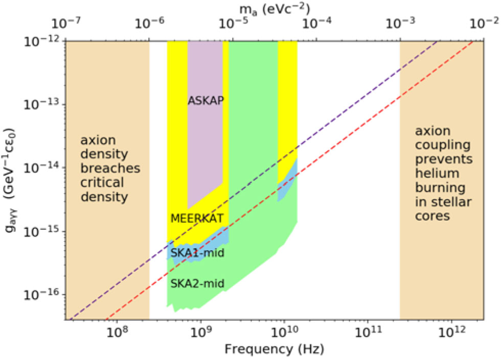
Figure 30. The coupling strength that could be probed by observing the interstellar medium across the frequency range accessible to ASKAP, MeerKAT and SKA-Mid. The sensitivities of SKA1-Mid and SKA2-Mid (blue and green, respectively) show considerable improvement on the pre-cursor telescopes, ASKAP (purple) and MeerKAT (yellow). The system temperature of the SKA is minimised between  $\sim\! 2 - 7$ GHz, corresponding to an axion mass of $\sim\! 8.26 - 28.91\ \mu$eVc–2 and providing a good opportunity for detection of both KSVZ and DFSZ axions. Figure reproduced from Kelley & Quinn (Reference Kelley and Quinn2017) by permission of the AAS.
5.3.6.4. Primordial BHs
The idea that PBHs can collapse in the early Universe out of small-scale density fluctuations (possibly originated during inflation) dates back to the early 1970s (see e.g., Hawking Reference Hawking1971; Carr & Hawking Reference Carr and Hawking1974). The PBH mass is of order the horizon mass at formation and can in principle span a very large range, from the Planck scale all the way up to  $\mathcal{O}(10 - 100)$ M $_{\odot}$. For masses larger than $10^{-17}$ M $_{\odot}$, the PBH evaporation lifetime (due to Hawking–Bekenstein radiation) is larger than the age of the Universe, and PBHs in that range can be a viable DM candidate, as first outlined by Chapline (Reference Chapline1975). However, observations have allowed astrophysical constraints to be placed on the mass ranges for which PBHs contribute significantly to the DM density, see Figure 31 (Carr et al. Reference Carr, Kohri, Sendouda and Yokoyama2010, Reference Carr, Kühnel and Sandstad2016).
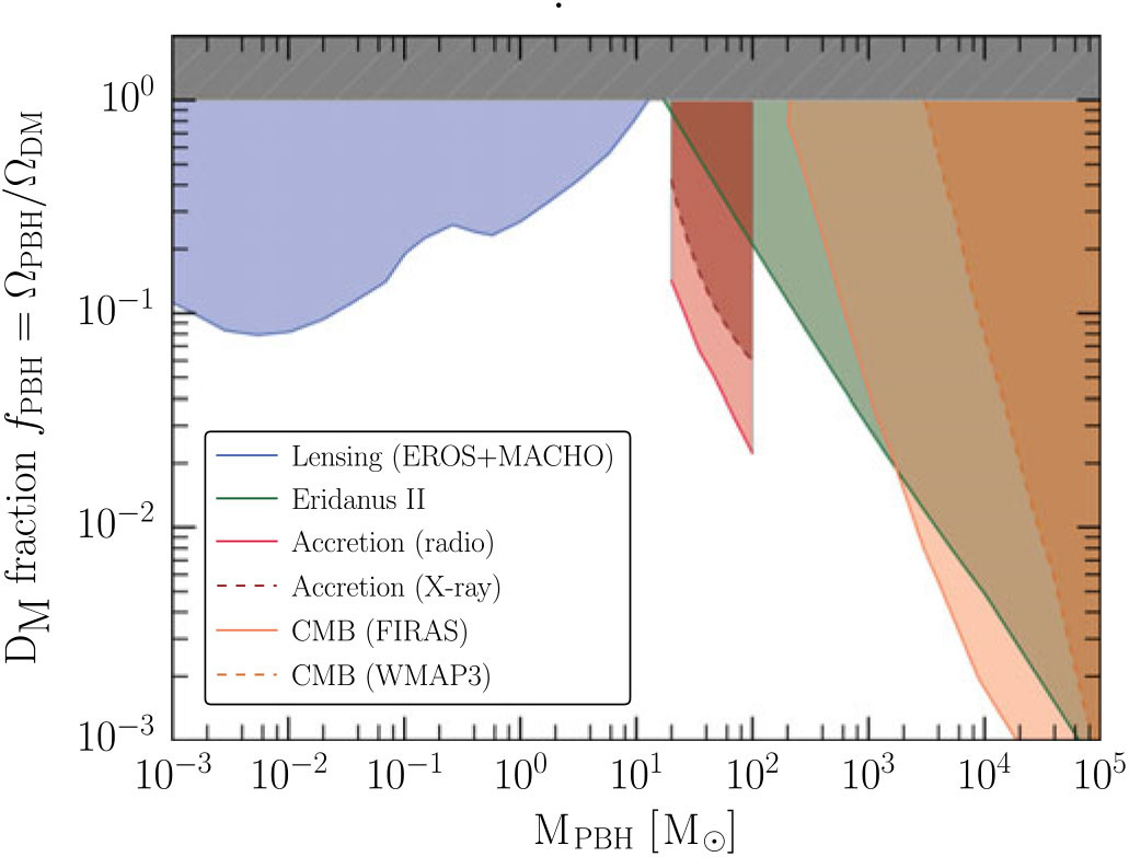
Figure 31. Summary of astrophysical constraints on PBHs in the mass range  ${\rm M} \in [10^{-3},\,10^5]\,{\rm M}_\odot$.
The recent LIGO detection of GWs from binary BH mergers has in particular prompted a renewed interest in the PBH mass window around  $10-100\ M_{\odot}$. The PBH merger rate was initially found to be consistent with that expected where PBHs make up all of the DM in the Universe (Bird et al. Reference Bird, Cholis, Muñoz, Ali-Haïmoud, Kamionkowski, Kovetz, Raccanelli and Riess2016), but subsequent analyses have contradicted this (Sasaki et al. Reference Sasaki, Suyama, Tanaka and Yokoyama2016; Ali-Haïmoud et al. Reference Ali-Haïmoud, Kovetz and Kamionkowski2017). SKA observations will allow this mass range to be further investigated through measurement of third-order Shapiro time delay induced by PBHs in MSP timing (Schutz & Liu Reference Schutz and Liu2017), or by looking for radio signatures both in the astronomical and cosmological context. On the cosmological side, the redshifted HI line is a very interesting observable. In fact, a population of PBHs is expected to accrete gas during the Dark Ages (see Section 2.2.1) and significantly change the reionisation history of the Universe: this effect can be probed by the SKA up to redshifts $\simeq\! 30$ (Poulin et al. Reference Poulin, Lesgourgues and Serpico2017). On the astronomical side, it is possible to look for radio and X-ray sources in the sky associated with a population of PBHs distributed in the Galaxy and accreting interstellar gas. There also remain other mass windows open in the context of DM, in particular the lunar mass range $10^{20}-10^{24}$ g and the atomic size range $10^{16}-10^{17}$ g. Pulsar timing with the SKA could be an important probe of the mass range $10^{22}-10^{28}$ g, even if these PBHs are highly subdominant (Kashiyama & Seto Reference Kashiyama and Seto2012).
Detecting PBHs using radio sources. PBHs can in principle be discovered by measuring the radio and X-ray emission produced by the accretion of interstellar gas onto these objects (Gaggero et al. Reference Gaggero2017). By comparing the predicted number of sources with astronomical catalogues, it may be possible to further constrain the fraction of DM in the form of PBHs. Even if they represent a subdominant contribution to DM, the SKA may still allow their discovery. Let us now demonstrate this claim in more detail, following the ideas and the approach of Gaggero et al. (Reference Gaggero2017). We focus on a small region of interest that includes the high-density region of the galactic ridge. The ridge is a promising region because it both represents a peak in the density of interstellar gas and therefore the strength of accretion, and resides near the GC where the DM density is also maximised. For radio emission, we assume that a jet is launched and adopt the universal empirical relation known as the fundamental plane (Plotkin et al. Reference Plotkin, Markoff, Kelly, Koerding and Anderson2012). We exploit this relation to compute the 5-GHz radio flux and assume a flat radio spectrum, such that  $F_{5\,{\rm GHz}}=F_{1.4\,{\rm GHz}}$. First, we consider the projected bound for the SKA1-Mid (band 2, $0.95 - 1.76$ GHz) point source sensitivity. Assuming PBHs of mass $\sim30 {\rm M}_{\odot}$ do account for all of the DM, and with a Monte Carlo simulation, we predict a detection of $\simeq\! 2\,000$ sources in our region of interest ( $<\!1^\circ$ away from the GC) for 1 h of exposure. In Figure 32, we show the predicted map of radio sources above the SKA1-Mid sensitivity threshold (for 1 h exposure) when the DM fraction is reduced to only 1%. Even in this case, corresponding to a subdominant population of PBHs, SKA1-Mid can detect a large number of sources. However, a detailed calculation of the SKA1-Mid detection sensitivity, correctly accounting for other radio source backgrounds, is postponed to a future work.
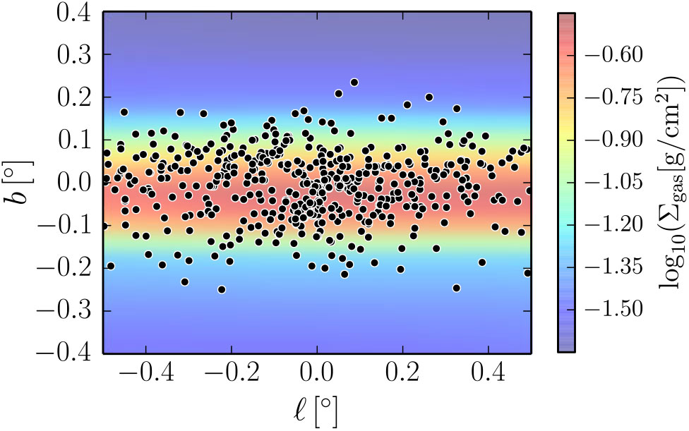
Figure 32. Radio sources above the SKA1-Mid point source sensitivity, for 1000 h of data taking, if PBHs are  $\sim 1\%$ of the DM.
PBHs and quantum gravity. Different approaches to quantum gravity converge in pointing out the possibility of instabilities of quantum gravitational origin that can manifest in an explosive event in a timescale shorter than the evaporation time (Gregory & Laflamme Reference Gregory and Laflamme1993; Kol & Sorkin Reference Kol and Sorkin2004). In particular, loop quantum gravity has recently provided a framework to compute explicitly this time (Christodoulou et al. Reference Christodoulou, Rovelli, Speziale and Vilensky2016). Loop quantum gravity removes the classical curvature singularities (Ashtekar & Bojowald Reference Ashtekar and Bojowald2006; Rovelli & Vidotto Reference Rovelli and Vidotto2013; Corichi & Singh Reference Corichi and Singh2016), such as the one at the BH centre, because of quantum spacetime discreteness. The consequences of this discreteness on the dynamics can be modelled at the effective level by an effective potential that prevents the gravitational collapse from forming the singularity and triggers a bounce. The bounce connects a collapsing solution of the Einstein equation, that is the classical BH, to an explosive expanding one, a white hole (Haggard & Rovelli Reference Haggard and Rovelli2015), through an intermediate quantum region. This process is a typical quantum tunnelling event, and the characteristic time at which it takes place, the hole lifetime, can be as a decaying time, similar to the lifetime of conventional nuclear radioactivity. The resulting picture is conservative in comparison to other models of non-singular BHs. The collapse still produces a horizon, but it is now a dynamical horizon with a finite lifetime, rather than a perpetual event horizon. The collapsing matter continues its fall after entering the trapping region, forming a very dense object whose further collapse is prevented by quantum pressure (referred to as a Planck Star; Rovelli & Vidotto Reference Rovelli and Vidotto2014).
While this fate should be generic for all BHs, it becomes experimentally relevant only for tiny and old BHs, being the primordial ones. The collapsing matter that forms PBHs in the radiation-dominated epoch is mainly constituted by photons. Seen from the centre of the hole, those photons collapse through the trapping region, then expand passing through an anti-trapping region and eventually exit the white hole horizon, always at the speed of light; the process is thus extremely fast. On the other hand, for an observer sitting outside the horizon, a huge but finite redshift stretches this time to cosmological times. This time, properly called the hole lifetime, as discussed before, has a minimal duration of  $M_{\rm BH}^2$ and a maximal duration below $M_{\rm BH}^3$. In analogy with standard quantum decay processes, one may expect the shortest possible time $M_{\rm BH}^2$ to be favoured.
Astrophysical signals produced in the explosive event associated with the BH decay could be detectable directly. Various signals can be expected (Barrau et al. Reference Barrau, Bolliet, Vidotto and Weimer2016, Reference Barrau, Martineau and Moulin2018a): (1) a high-energy signal determined by the temperature of the photons emitted, (2) a signal determined by the size of the hole exploding, (3) a signal in the radio due to the possible presence of magnetic fields around the exploding hole, and (4) the emission in GWs. The peak of signal (2) falls at millimetre wavelengths; however, the full distribution of events is accessible to SKA1-Mid (Barrau et al. Reference Barrau, Moulin and Martineau2018b). Interestingly, the signal presents a peculiar wavelength–distance relation (Barrau et al. Reference Barrau, Rovelli and Vidotto2014), which allows it to be discriminated from other astrophysical sources, either via direct detection, or via the resulting background radiation (Barrau et al. Reference Barrau, Bolliet, Vidotto and Weimer2016) that SKA IM may detect, especially with the improved sensitivity of SKA2-Mid.
Signal (3) is fully within the frequency range of SKA1-Mid and SKA2-Mid. The interaction of signal (1) with the ionised interstellar medium produces a radio pulse at a frequency  $\sim\!1$ GHz (Rees Reference Rees1977; Blandford Reference Blandford1977). Interestingly, this signal has similar properties to those of fast radio bursts (FRBs). In this case, the emission mechanism relies on the presence of a shell of relativistic charged particles produced in the explosion. The shell behaves as a superconductor that expels the interstellar magnetic field from a spherical volume centred on the original BH site (Cutchin et al. Reference Cutchin, Simonetti, Ellingson, Larracuente and Kavic2016).
Finally, PBH decay has the peculiar property of lowering the DM energy density content of the Universe, since the decay effectively converts DM into radiation. This affects the galaxy number count in large-scale galaxy surveys, in particular measurements of galaxy clustering, galaxy lensing, and RSDs (Raccanelli et al. Reference Raccanelli, Vidotto and Verde2018). The LSS surveys performed by the SKA will provide key data in this respect by detecting individual galaxies in the radio continuum (Jarvis et al. Reference Jarvis, Bacon, Blake, Brown, Lindsay, Raccanelli, Santos and Schwarz2015b).
5.4. Astroparticle physics
In this section, we discuss how the SKA can constrain the masses of photons (Section 5.4.3) and neutrinos (Sections 5.4.1 and 5.4.2). We also consider the problem of cosmic ray acceleration in magnetic fields and how the SKA can improve the relatively little knowledge we have about magnetic fields (Section 5.4.4).
5.4.1. Constraining the neutrino mass
Determining the sum of the neutrino masses and their hierarchy is one of the most important tasks of modern physics. Unfortunately, setting upper bounds from laboratory experiments is very challenging. It is expected that in the near future katrinFootnote p will set an upper limit of  $M_\nu=\sum_i m_{\nu_i}<0.6$ eV. A different way to determine the sum of the neutrino masses is through cosmological observables, where their very large thermal velocities (in contrast with the assumed negligible ones for CDM) produce a clear neutrino signature, in particular a suppression of power on small scales in the matter power spectrum. Understanding and measuring this effect is also important for dark energy and GR tests, as models of modified gravity or interacting DM/energy also lead to modifications of small-scale power (see e.g., Wright et al. Reference Wright, Winther and Koyama2017).
Current constraints on the sum of the neutrino masses, arising by combining data from the CMB, galaxy clustering, and/or the Lyman- $\alpha$ forest, are $M_\nu\lesssim0.12$ eV (Riemer-Sø rensen et al. 2014; Palanque-Delabrouille et al. Reference Palanque-Delabrouille2015; Cuesta et al. Reference Cuesta, Niro and Verde2016; Vagnozzi et al. Reference Vagnozzi, Giusarma, Mena, Freese, Gerbino, Ho and Lattanzi2017). One would naively expect that those constraints can be improved using galaxy clustering at higher redshifts, since the available volume is much larger, the non-linear clustering effects are weaker, and the effects of dark energy will be smaller.
The possibility of using high-redshift optical galaxy surveys (combined with CMB data in order to lift parameter degeneracies) to provide precision measurements of the neutrino masses is not new (see e.g., Takada et al. Reference Takada, Komatsu and Futamase2006). However, the detection of galaxies at high redshifts becomes more difficult and expensive, and shot noise effects may dominate. In Takada et al. (Reference Takada, Komatsu and Futamase2006), a space-based galaxy survey with a 300-deg $^2$ sky coverage at redshifts $3.5<z<6.5$ (assuming a very large number density and bias of the galaxy tracers) was found to be able to measure the neutrino mass with $\sigma(m_{\nu,{\, \rm tot}}) = 0.025$ eV combined with CMB data.
Another possibility is to map the LSS of the Universe through 21-cm IM. Given the fact that neutrinos modify the abundance of halos (Castorina et al. Reference Castorina, Sefusatti, Sheth, Villaescusa-Navarro and Viel2014; Costanzi et al. Reference Costanzi, Villaescusa-Navarro, Viel, Xia, Borgani, Castorina and Sefusatti2013), their clustering (Villaescusa-Navarro et al. Reference Villaescusa-Navarro, Marulli, Viel, Branchini, Castorina, Sefusatti and Saito2014; Castorina et al. Reference Castorina, Sefusatti, Sheth, Villaescusa-Navarro and Viel2014) and also the internal halo properties such as concentration (Villaescusa-Navarro et al. Reference Villaescusa-Navarro, Bird, Peña-Garay and Viel2013), it is expected that they will also leave a signature on the abundance and spatial distribution of cosmic HI in the post-reionisation era. This has been explicitly checked by means of hydrodynamic simulations by Villaescusa-Navarro et al. (Reference Villaescusa-Navarro, Bull and Viel2015). The key point to understand the impact of neutrino masses on the abundance and clustering properties of HI is the fact that halos of the same mass have very similar HI content, independently of the sum of the neutrino masses. The results show that in cosmologies with massive neutrinos the abundance of cosmic HI will be suppressed with respect to the equivalent massless neutrino model. At the same time, the presence of massive neutrinos will make the HI more clustered.
Villaescusa-Navarro et al. (Reference Villaescusa-Navarro, Bull and Viel2015) investigated the constraints that IM observations using SKA1 can place on the sum of the neutrino masses. They considered a deep survey by SKA1-Low covering  $\simeq20$ deg $^2$ with $10\,000$ h using interferometry over a bandwidth covering redshifts $z\in[3-6]$, and a wide SKA1-Mid survey covering $20\,000$ deg $^2$ over $10\,000$ h using the single-dish mode of observation from $z=0$ to $z=3$. As shown in Figure 33, the neutrino mass can be constrained with $\simeq0.09$ eV ( $1\sigma$). It is important to note that, for the given observing time, the constraints from SKA1-Low remain practically constant up to a survey area of 100 deg $^2$, and similarly for SKA1-Mid down to $2\,000$ deg $^2$. The constraints are more sensitive to the total available observation time. By combining IM observations with data from Planck and optical galaxy surveys like Euclid the uncertainty can shrink to $\simeq0.03$ eV ( $1\sigma$), which is very competitive with respect to any other probe such as galaxy clustering probes or the Lyman- $\alpha$ forest.
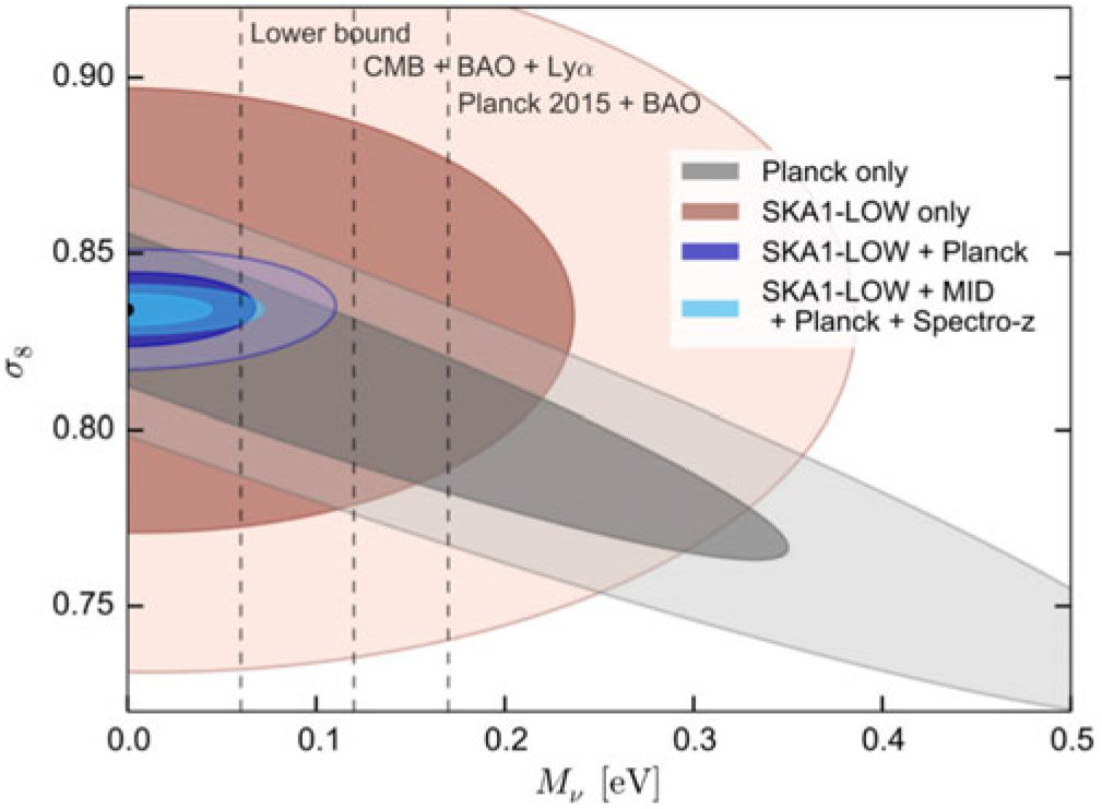
Figure 33. Constraints on the  $M_\nu-\sigma_8$ plane from Planck (grey), SKA1-Low (brown), SKA1-Low + Planck (dark blue) and SKA1-Low + SKA1-Mid + Planck + Euclid (light blue). The vertical dashed lines indicate the minimum sum of the neutrino masses from neutrino oscillations together with recent bounds from cosmological probes. Adapted from Villaescusa-Navarro et al. (Reference Villaescusa-Navarro, Bull and Viel2015).
5.4.2. Constraining neutrino properties with SKA voids
Future SKA HI galaxy surveys will offer an unprecedented spectroscopic view of both large and small scales in the cosmic web. This will allow the identification and mapping of around  $10^5 - 10^6$ voids in the galaxy distribution, from the smallest to the largest voids in the Universe (Sahlén & Silk Reference Sahlén and Silk2018). Figure 34 shows the expected limiting void radii for a selection of future large, spectroscopic surveys (we limit the discussion to spectroscopic surveys to minimise the impact of redshift-space systematics). The number counts (Pisani et al. Reference Pisani, Sutter, Hamaus, Alizadeh, Biswas, Wandelt and Hirata2015; Sahlén et al. Reference Sahlén, Zubeldia and Silk2016), shapes (Massara et al. Reference Massara, Villaescusa-Navarro, Viel and Sutter2015), RSDs (Sutter et al. Reference Sutter, Pisani, Wandelt and Weinberg2014), and lensing properties (Spolyar et al. Reference Spolyar, Sahlén and Silk2013) of voids are examples of sensitive void probes of cosmological parameters. Voids are particularly sensitive to the normalisation and shape of the matter power spectrum, and the effects of screened theories of gravity which exhibit a modification to GR in low-density environments (Voivodic et al. Reference Voivodic, Lima, Llinares and Mota2017). This is because void distributions contain objects ranging from the linear to the non-linear regimes, across both scale and redshift. SKA2 will also reach well into the void-in-cloud limit across a wide range of redshifts, allowing a detailed study of this theoretically uncertain process whereby small voids disappear through the collapse of the larger overdensities within which they arise.
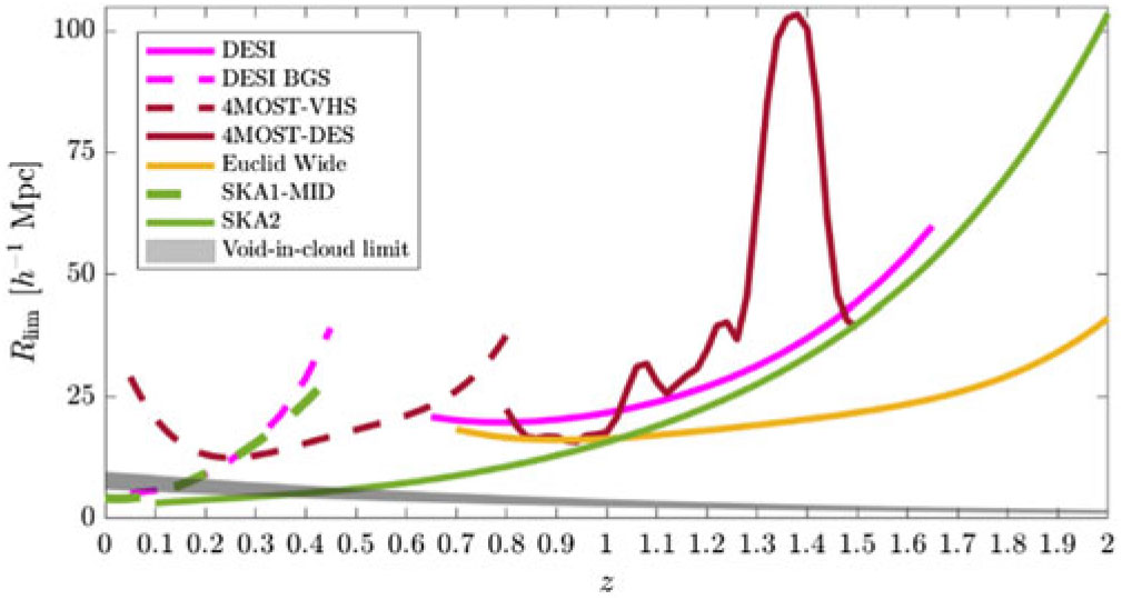
Figure 34. Expected limiting void radii for future spectroscopic galaxy surveys (not including quasars) across the corresponding survey redshift ranges. An approximate void-in-cloud limit is indicated (shaded), below which theoretical predictions are uncertain as regards to what extent voids inside overdensity clouds disappear due to halo collapse of the overdensity.
As a particular case for the SKA, we consider number counts of voids and forecast cosmological parameter constraints from future SKA surveys in combination with Euclid, using the Fisher matrix method. Massive neutrinos affect void and galaxy cluster distributions by shifting the turnover scale in the matter power spectrum as set by the redshift of matter radiation equality. Their free streaming also suppresses power on the neutrino free-streaming scale (set by the neutrino masses), which significantly affects the number counts and shapes of voids (Massara et al. Reference Massara, Villaescusa-Navarro, Viel and Sutter2015) and the number counts of clusters (Brandbyge et al. Reference Brandbyge, Hannestad, Haugbølle and Wong2010).
We consider a flat wCDM cosmology with massive neutrinos described by the sum of neutrino masses  $\Sigma m_{\nu}$. The void distribution is modelled following Sahlén et al. (Reference Sahlén, Zubeldia and Silk2016), Sahlén & Silk (Reference Sahlén and Silk2018), and Sahlén (Reference Sahlén2019), also taking into account the galaxy density and bias for each survey (Yahya et al. Reference Yahya, Bull, Santos, Silva, Maartens, Okouma and Bassett2015; Raccanelli et al. Reference Raccanelli, Montanari, Bertacca, Doré and Durrer2016c). The results are shown in Figure 35 (see caption for survey and model assumptions). The combined SKA1-Mid & Euclid void number counts could achieve a precision $\sigma(\Sigma m_{\nu}) = 0.02$ eV, marginalised over all six other parameters. No additional priors are included. The SKA2 void number counts could improve on this by a factor of two, potentially distinguishing $\Sigma m_{\nu} = 0.06$ eV from $\Sigma m_{\nu} = 0.1$ eV and allowing for a determination of the neutrino hierarchy characterised by those masses (inverted and normal, respectively). Using the powerful degeneracy-breaking complementarity between clusters of galaxies and voids (Sahlén et al. Reference Sahlén, Zubeldia and Silk2016; Sahlén & Silk Reference Sahlén and Silk2018; Sahlén Reference Sahlén2019), SKA2 voids + Euclid clusters number counts could reach as low as $\sigma(\Sigma m_{\nu}) = 0.002$ eV. These forecasts are highly competitive with expectations for planned Stage IV CMB experiments/probes (e.g., Pan & Knox Reference Pan and Knox2015).
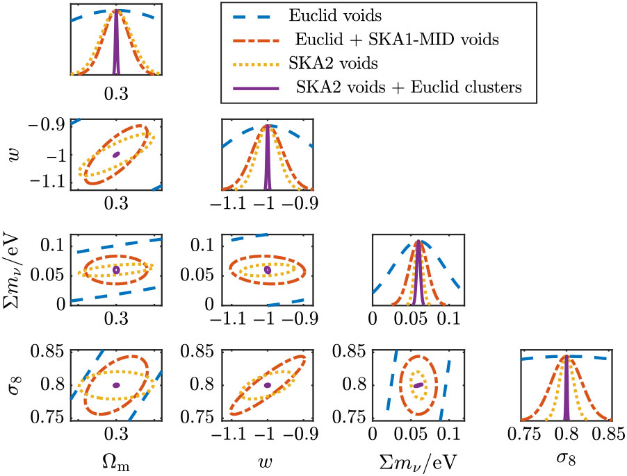
Figure 35. Forecast parameter constraints (95% confidence levels) for a flat wCDM model with massive neutrinos. Note the considerable degeneracy breaking between the Euclid and SKA1 void samples, and between the SKA2 void and Euclid cluster samples. SKA1-Mid covers 5 000 deg $^2$,
$^2$,  $z = 0-0.43$. SKA2 covers 30 000 deg $^2$,
$^2$,  $z=0.1-2$. Euclid voids covers 15 000 deg $^2$,
$^2$,  $z=0.7-2$. Euclid clusters covers 15 000 deg $^2$,
$^2$,  $z=0.2-2$. The fiducial cosmological model is given by
  $\{\Omega_{\rm m} = 0.3, w = -1, \Sigma m_{\nu} = 0.06 \,{\rm eV}, \sigma_8
= 0.8, n_{\rm s} = 0.96, h = 0.7, \Omega_{\rm b} = 0.044\}$. We have also marginalised over uncertainty in void radius and cluster mass (Sahlén & Silk Reference Sahlén and Silk2018), and in the theoretical void distribution function (Pisani et al. Reference Pisani, Sutter, Hamaus, Alizadeh, Biswas, Wandelt and Hirata2015).
$\{\Omega_{\rm m} = 0.3, w = -1, \Sigma m_{\nu} = 0.06 \,{\rm eV}, \sigma_8
= 0.8, n_{\rm s} = 0.96, h = 0.7, \Omega_{\rm b} = 0.044\}$. We have also marginalised over uncertainty in void radius and cluster mass (Sahlén & Silk Reference Sahlén and Silk2018), and in the theoretical void distribution function (Pisani et al. Reference Pisani, Sutter, Hamaus, Alizadeh, Biswas, Wandelt and Hirata2015).
5.4.3. Measuring the photon mass with FRBs
FRBs are short, dispersed spikes of radio waves, typically lasting a few milliseconds at  $\sim$ GHz frequencies (Lorimer et al. Reference Lorimer, Bailes, McLaughlin, Narkevic and Crawford2007; Thornton et al. Reference Thornton2013). They appear to come from powerful events at cosmological distances with their cause still unknown (Katz Reference Katz2016). Despite our ignorance of their origin, FRBs can be used to study fundamental physics, particularly in setting upper limits on the mass of the photon (Wu et al. Reference Wu2016; Bonetti et al. Reference Bonetti, Ellis, Mavromatos, Sakharov, Sarkisyan-Grinbaum and Spallicci2016, Reference Bonetti, Ellis, Mavromatos, Sakharov, Sarkisyan-Grinbaum and Spallicci2017; Shao & Zhang Reference Shao and Zhang2017).
If photons are massive, the speed of light will be energy-dependent (in a Lorentz-invariant theory), with high-energy photons travelling faster. Thus, low-energy photons will have a time delay after they traverse a fixed distance. Because of (1) the short time duration ( $\sim$ ms), (2) the large travelling distance ( $\sim$ Gpc), and (3) the low energy of photons ( $\sim\!\mu$eV), FRBs are among the best celestial objects to constrain the photon mass, $m_\gamma$ (Shao & Zhang Reference Shao and Zhang2017). Individual sources with redshift measurements have been used to obtain a limit of $m_\nu < \mathcal{O}(10^{-50})$ kg (Wu et al. Reference Wu2016; Bonetti et al. Reference Bonetti, Ellis, Mavromatos, Sakharov, Sarkisyan-Grinbaum and Spallicci2016, Reference Bonetti, Ellis, Mavromatos, Sakharov, Sarkisyan-Grinbaum and Spallicci2017). Nevertheless, measurements of FRB redshifts are rare (Chatterjee et al. Reference Chatterjee2017) and consequently a Bayesian framework, where FRBs with and without redshift measurement equally contribute to the constraint, was used to obtain the currently best limit from the kinematics of light propagation (Shao & Zhang Reference Shao and Zhang2017).
In January 2017, the Commensal Real-time ASKAP Fast Transients survey found a FRB in a 3.4-d pilot survey (Bannister et al. Reference Bannister2017). Such a survey benefits greatly from the large field of view with the phased-array-feed technology. The CHIME will also find many more FRBs (CHIME/FRB Collaboration et al. 2018; Boyle et al. Reference Boyle2018), while when SKA2 is operating, FRBs will be detected daily. These FRBs will contribute to an even tighter limit on the photon mass or may even discover new physics beyond the standard model if photons are indeed massive.
5.4.4. The non-thermal Universe
Continuum observations with the SKA will allow profound insights into the non-thermal Universe. This encompasses sources of the energy density that stem from magnetic fields, non-thermal particles (also called cosmic rays), and turbulent motions. In spiral galaxies, these non-thermal components dominate the total energy density. Also on larger scales, in the cosmic web of galaxy clusters and filaments, there is ample evidence of substantial non-thermal components. An example is shown in Figure 36, which shows a multi-wavelength image of the ‘toothbrush’ relic, a 3-Mpc long diffuse radio source, located at the periphery of a merging galaxy cluster (van Weeren et al. 2016). At radio wavelengths, these non-thermal components are mostly observed via the synchrotron emission that is produced by relativistic electrons with Lorentz factors of a few hundred gyrating in magnetic fields (see also Section 5.3.1). However, the origins of both the magnetic fields and the relativistic particles are unknown.
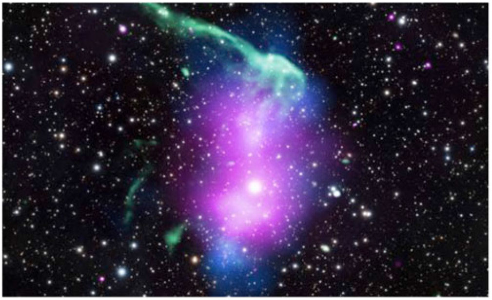
Figure 36. Multi-wavelength image of the so-called ‘toothbrush’ radio relic. The green colours show the radio image (LOFAR), the magenta the X-ray (Chandra) view and the white the optical data (Subaru) (van Weeren et al. 2016).
The diffuse radio sources observed in galaxy clusters span vast scales of up to several Mpc. The short synchrotron cooling time of the electrons implies that they must be injected in situ by a process operating over the same spatial scale as the source itself. The plasmas in which radio relics and halos occur are collisionless and have number densities of  $10^{-4} -
10^{-3}$ cm–3. Moreover, the magnetic fields have strengths of around a few
$10^{-4} -
10^{-3}$ cm–3. Moreover, the magnetic fields have strengths of around a few  $\mu$G, leading to a substantially weaker magnetic pressure than the thermal pressure. Similar conditions are unattainable in a laboratory on Earth and hence can only be studied remotely through astronomical observations.
Cosmological simulations predict that the largest part of radio relics and halos have not been discovered yet, since their large size and low surface brightness makes them difficult to find (e.g., Nuza et al. Reference Nuza, Gelszinnis, Hoeft and Yepes2017; Wittor et al. Reference Wittor, Vazza and Brüggen2017). Yet, through the study of these objects, one hopes to find (1) a process that can generate magnetic fields that fill large volumes (probably) in very low-density cosmic environments, and (2) processes that can accelerate electrons to relativistic energies such that they fill an entire galaxy cluster or operate at the outskirts of clusters. The main candidates are shock waves and turbulence, but it is not known whether low-Mach number shocks are efficient enough, or what fraction of the magnetic field is produced by the shock wave itself and what part is merely amplified via compression.
The SKA will be able to probe the cosmic filaments that are predicted to contain most of the baryons in the Universe (Davé et al. Reference Davé2001). Very little is known about these filaments, since the thermal state of the baryons and their low column densities makes them very hard to observe, but they are expected to be sheathed by accretion shocks for which both the continuum and polarised emission could be detectable. Provided that the shocks in this extreme environment are at least as efficient as cluster shocks in accelerating relativistic electrons, we have predicted the flux densities of the synchrotron radiation that could be detected by the SKA for magnetic fields of order  $\sim\! 0.01-0.1$ $\mu$G.
In Figure 37, we show the predicted synchrotron signal from shock-accelerated relativistic electrons in a  $5 \times 15$ degree region from a cosmological simulation, as observed assuming the typical sensitivities of current and future technologies. The region was extracted from a cosmological magnetohydrodynamic (MHD) simulation performed with the ENZO code (Bryan et al. Reference Bryan2014). The acceleration efficiency of electrons by shocks is tuned to reproduce the radio emission observed at radio relics in the intracluster medium (Vazza et al. Reference Vazza, Ferrari, Brüggen, Bonafede, Gheller and Wang2015).Footnote q This mock observation illustrates the large jump in sensitivity to the diffuse and shocked cosmic web that we expect to achieve with SKA1-Low, allowing us to greatly improve our present view of EG magnetic fields beyond the innermost regions of galaxy clusters. There are strong indications that both radio relics and halos are in fact made up of quite distinct subclasses of sources (e.g., de Gasperin et al. Reference de Gasperin, Ogrean, vanWeeren, Dawson, Brüggen, Bonafede and Simionescu2015; van Weeren et al. 2017). The improved sensitivity of the SKA will provide sufficient statistics to study and distinguish between the various particle acceleration and re-acceleration scenarios.
Figure 37. Mock observations of a  $5 \times 15$ degree area including galaxy clusters and filaments, assuming the sensitivity of the NVSS survey with the Very Large Array at $1.4$ GHz (top) and with the sensitivity of a survey with SKA1-Low at 110 MHz (bottom) in units of $\rm Jy/arcsec^2$. The underlying cosmological simulations are part of the CHRONOS++ suite of MHD simulations with the ENZO code and was run on the Piz-Daint computer cluster at CSCS in Lugano (Vazza et al. Reference Vazza, Brüggen, Gheller and Wang2014).
The SKA will be able to detect cosmic filaments if the magnetic field energy density is at the level of a few percent of the thermal energy density (Vazza et al. Reference Vazza, Ferrari, Brüggen, Bonafede, Gheller and Wang2015). Observations below  $\approx\! 200$ MHz are best suited to detect the large-scale diffuse emission produced by cosmological shock waves. These shocks are characterised by a flat emission spectrum and show flux densities of $\sim\mu$Jy/arcsec $^2$ at low redshifts. Because of cosmological dimming, most of the detectable radio emission is caused by structures at $z \leq 0.1$. Especially at high frequencies, the detection of nearby filaments ( $z \leq 0.02$) is difficult because of the lack of short baselines. The range of magnetic fields that should ensure a systematic detection of the cosmic web at the periphery of galaxy clusters is in line with the magnetic field detected along an accreting group in the nearby Coma galaxy cluster (Bonafede et al. Reference Bonafede, Vazza, Brüggen, Murgia, Govoni, Feretti, Giovannini and Ogrean2013) and can be achieved either via a small-scale dynamo or via release of magnetic fields by nearby galaxies/AGN. Assessing which of these mechanism(s) is responsible for the magnetisation in such rarefied cosmic environments is an exciting and important challenge for the SKA.
5.5. Summary
It is clear that the SKA will provide significant advancements in our understanding of astronomical, cosmological, and even particle theories. The wide range of opportunities set out in this section focus only on the fields of DM and astroparticle physics and demonstrate the power of this new technology. Just the increased observability of high-energy objects such as pulsars, binary stars, and AGN, and the ability to trace back to extremely high redshift offers a wealth of new data that will contribute to a number of important and groundbreaking discoveries.
HI IM in particular is a new and powerful tool for mapping the structure formation of the Universe. It will provide insight on the clustering properties and thermal characteristics of DM. The increased sensitivity also opens the door for DM particle searches as well as new experiments for constraining standard model particle properties such as the neutrino mass. It may even offer the opportunity to test new quantum gravity and string theories through observations of PBHs and binary pulsars.
6. Conclusions
Physicists seek to understand the nature of matter, energy, and spacetime, plus how the three of these have interacted over cosmic time. While great strides have come from terrestrial and solar system experiments, it is increasingly clear that immense progress lies ahead through studying the cosmos.
Modern radio telescopes now have the capability to gather enormous statistical samples of celestial objects and to make ultra-precise measurements of astrophysical effects. In this paper, we have explained the many ways in which the SKA will push far beyond the current frontiers in these areas and will allow us to ask and answer new questions about cosmology, gravity, DM, dark energy, and more. The SKA will not just be a revolutionary facility for astronomy, but will also be an extraordinary machine for advancing fundamental physics.
Acknowledgements. The workshop ‘Fundamental Physics with the Square Kilometre Array’ was made possible through the generous support of the Dunlap Institute for Astronomy and Astrophysics, the Square Kilometre Array Organisation, SKA South Africa, the ARC Centre of Excellence for All-Sky Astrophysics (CAASTRO), the International Centre for Radio Astronomy Research (ICRAR), the National Institute for Theoretical Physics (NITheP), the Netherlands Research School for Astronomy (NOVA), and the NRF/DST South African Research Chairs Initiative (SARChI).
Individually, the authors recognise a number of collaborators, institutions, and funding bodies for their support, namely:
A. Weltman acknowledges financial support from the DST/NRF South African Research Chairs programme as well as the Institute for Advanced Study, Princeton and the Flatiron Institute through the Simons Foundation.
P. Bull’s research was supported by an appointment to the NASA Postdoctoral Program at the Jet Propulsion Laboratory, California Institute of Technology, administered by Universities Space Research Association under contract with NASA.
S. Camera is supported by MIUR through Rita Levi Montalcini project ‘prometheus—Probing and Relating Observables with Multi-wavelength Experiments To Help Enlightening the Universe’s Structure’, and by the ‘Departments of Excellence 2018–2022’ Grant awarded by MIUR (L. 232/2016).
H. Padmanabhan’s research was supported by the Tomalla Foundation.
J. R. Pritchard is pleased to acknowledge support from the European Research Council under ERC grant number 638743-FIRSTDAWN.
A. Racanelli has received funding from the People Programme (Marie Curie Actions) of the European Union H2020 Programme under REA grant agreement number 706896 (COSMOFLAGS). Funding for this work was partially provided by the Spanish MINECO under MDM-2014-0369 of ICCUB (Unidad de Excelencia ‘Maria de Maeztu’).
E.Athanassoula and A. Bosma thank the Action Spécifique SKA-LOFAR of CNRS/INSU for financial support.
For R. Barkana, this project/publication was made possible through the support of a grant from the John Templeton Foundation; the opinions expressed in this publication are those of the authors and do not necessarily reflect the views of the John Templeton Foundation.
G. Bertone, F. Calore, R.M.T. Connors, and D. Gaggero acknowledge collaboration with M. Lovell, S. Markoff, and E. Storm.
Camille Bonvin acknowledges partial support by INAF-Direzione Scientifica and by ASI through ASI/INAF Agreement 2014-024-R.1 for the Planck LFI Activity of Phase E2.
M. Brüggen’s work was strongly supported by computing resources from the Swiss National Supercomputing Centre (CSCS) under projects ID s585 and s701. F. Vazza acknowledges financial support from the European Union’s Horizon 2020 research and innovation programme under the Marie-Sklodowska-Curie grant agreement No. 664931 and the ERC Starting Grant ‘MAGCOW’, No. 714196. They acknowledge allocations 9059 on supercomputers at the NIC of the Forschungszentrum Jülich. Computations described in their work were performed using the ENZO code, which is the product of a collaborative effort of scientists at many universities and national laboratories.
C. Burigana and T. Trombetti acknowledge partial support from the INAF PRIN SKA/CTA project FORmation and Evolution of Cosmic STructures (FORECaST) with Future Radio Surveys.
C. Weniger and F. Calore acknowledge collaboration with F. Donato, M. Di Mauro, and J. W. T. Hessels. Their research is funded by NWO through an NWO Vidi research grant.
J.A.R. Cembranos and Á. de la Cruz-Dombriz acknowledge financial support from the Consolider-Ingenio MULTIDARK CSD2009-00064 project.
A. de la Cruz-Dombriz acknowledges financial support from projects Consolider-Ingenio MULTIDARK CSD2009-00064. FPA2014-53375-C2-1-P Spanish Ministry of Economy and Science, FIS2016-78859-P European Regional Development Fund and Spanish Research Agency (AEI), CA15117 CANTATA and CA16104 COST Actions EU Framework Programme Horizon 2020, CSIC I-LINK1019 Project, Spanish Ministry of Economy and Science, University of Cape Town Launching Grants Programme.
A. Dombriz (grant numbers 99077, CSUR150628121624, IFR170131220846) P. Dunsby, J. Larena, Y-z Ma (grant numbers 104800, 105925) are supported by the National Research Foundation (South Africa).
M. Méndez-Isla acknowledges financial support from the University of Cape Town Doctoral Fellowships and the Erasmus+ Alliance4Universities Mobility Programme.
S. Camera, M. Regis, and N. Fornengo are supported by: the research grant The Anisotropic Dark Universe, number CSTO161409, funded under the programme CSP-UNITO Research for the Territory 2016 by Compagnia di Sanpaolo and University of Torino; the research grants TAsP (Theoretical Astroparticle Physics) and InDark (Inflation, DM and the LSS of the Universe) funded by the Istituto Nazionale di Fisica Nucleare (INFN). Their research is also funded by MIUR through the Rita Levi Montalcini project ‘prometheus—Probing and Relating Observables with Multi-wavelength Experiments To Help Enlightening the Universe’s Structure’.
The contribution of S. D. Mohanty to this paper is supported by NSF Grants PHY-1505861 and HRD-0734800.
R. Maartens is supported by the South African SKA Project and by the UK STFC, Grant ST/N000668/1.
D. Parkinson acknowledges support of the Australian Research Council through the award of a Future Fellowship [Grant No. FT130101086].
A. Pourtsidou’s work for this project was partly supported by a Dennis Sciama Fellowship at the University of Portsmouth.
M. Regis acknowledges support by the Excellent Young PI Grant: ‘The Particle Dark-matter Quest in the Extragalactic Sky’ funded by the University of Torino and Compagnia di San Paolo, by ‘Deciphering the high-energy sky via cross correlation’ funded by Accordo Attuativo ASI-INAF No. 2017-14-H.0., and by the project ‘Theoretical Astroparticle Physics (TAsP)’ funded by the INFN.
M. Sahlén is supported by Olle Engkvist Foundation. Sakellariadou is partially supported by STFC (UK) under the research grant ST/L000326/1.
T. Venumadhav acknowledges support from the Schmidt Fellowship and the Fund for Memberships in Natural Sciences at the Institute for Advanced Study.
F. Vidotto acknowledges support by grant IT956-16 of the Basque Government and by grant FIS2017-85076-P (MINECO/AEI/FEDER, UE).
The work of F. Villaescusa-Navarro is supported by the Simons Foundation.
Y. Wang is supported by the National Natural Science Foundation of China (NSFC) under Grants No. 11973024, No. 91636111, No. 11690021, No. 11503007, and ‘the Fundamental Research Funds for the Central Universities’ under Grant No. 2019kfyRCPY106.
L. Wolz is supported by an ARC Discovery Early Career Researcher Award (DE170100356). Part of her research was also supported by the Australian Research Council Centre of Excellence for All-sky Astrophysics (CAASTRO), through project number CE110001020.
B. M. Gaensler acknowledges support from: the Dunlap Institute of Astronomy and Astrophysics, funded through an endowment established by the David Dunlap family and the University of Toronto; the Natural Sciences and Engineering Research Council of Canada (NSERC) through grant RGPIN-2015-05948; and of the Canada Research Chairs programme.
The use of the Planck Legacy ArchiveFootnote r is acknowledged. We acknowledge use of the HEALPixFootnote s (Górski et al. 2005) software and analysis package.


