


1. Introduction
Molecular bands in the spectra of cool stars need to be considered in the calculation of synthetic spectra of cool stars, first of all because they are present all over the spectra, affecting considerably the continuum, and because there are several strong lines. Bands involving C, N, O, in particular, are key indicators of many important aspects of both stellar evolution and chemical evolution. For example, photometric filters placed to measure CH, NH, CN, OH, as used in Piotto et al. (Reference Piotto, Milone and Bedin2015), can reveal multiple stellar populations in globular clusters.
The main nitrogen indicators used in the literature are CN bands, among which the strongest ones are in the near-UV, in particular CN(0,0) at 388.3 nm. For the use of CN, one has to previously derive C, available in the optical from the CH G-bandhead at 431 nm or a weak C2(0,0) bandhead at 563.5 nm. In the near-UV, there is the unique available strong NH bandhead at 336 nm. The NH band measurement in important samples would allow a direct measurement of nitrogen (e.g. Pasquini et al. Reference Pasquini, Ecuvillon, Bonifacio and Wolff2008). Note on the other hand that discrepancies have been found in the nitrogen abundances derived from CN and NH bandheads, still unsolved (see Spite et al. Reference Spite2005).
Oxygen has several strong OH lines occurring in the near-UV, at λ ≲ 330 nm, and in the near-infrared (NIR) in the H band. In metal-poor turn-off dwarf stars, the UV OH lines are the only measurable oxygen indicator. Furthermore, molecular bands of CH and CN in the visible and NIR are the best way of deriving the isotopic composition of, in particular, 12C/13C (e.g. Smith, Terndrup, & Suntzeff Reference Smith, Terndrup and Suntzeff2002), which is an indicator of stellar mixing (e.g. Smiljanic et al. Reference Smiljanic, Gauderon, North, Barbuy, Charbonnel and Mowlavi2009).
Therefore, the inclusion of molecular lines in synthetic spectra calculations of stars cooler than ≲7 000 K is of utmost importance. Line lists of molecular bands come however in different formats, and as well the different codes use these lists adapted in different ways. The main difference in using molecular line lists is the use of either the Einstein A coefficients, such as given in Goorvitch (Reference Goorvitch1994) for the NIR lines of CO X1Σ+ system, which are a sum of all ingredients, or when this is not available, the different constituents that produce the line. In the present paper we aim to show how to use these different data.
Codes for spectrum synthesis available include about a dozen of them, among which Synthe (Kurúcz Reference Kurúcz1970, Reference Kurúcz1993a), Moog (Sneden Reference Sneden1973), the codes Bsyn (Edvardsson et al. Reference Edvardsson, Andersen, Gustafsson, Lambert, Nissen and Tomkin1993), and Turbospectrum (Alvarez & Plez Reference Alvarez and Plez1998), from the Uppsala group, and SME (Valenti & Piskunov Reference Valenti and Piskunov1996; Piskunov & Valenti Reference Piskunov and Valenti2017), among a few others. In the present paper, we give details on the updated version of the spectrum synthesis code Pfant, which is now available online.
In Section 2 we describe the calculation of molecular lines of diatomic molecules. In Section 3 we describe the spectrum synthesis code Pfant and the line lists used. In Section 4 a short summary is given.
2. Molecular absorption coefficient
In the 1960s and early 1970s a few authors provided the basis for the understanding and correct calculation of molecular line formation. There are some inconsistencies in normalisation matters among these papers, which made the subject a hot topic at that time. These include Schadee (Reference Schadee1964, Reference Schadee1967, Reference Schadee1975, Reference Schadee1978), Tatum (Reference Tatum1967), and Whiting & Nicholls (Reference Whiting and Nicholls1974). A particularly clear work on normalisation factors was given later by all these authors gathered in Whiting et al. (Reference Whiting, Schadee, Tatum, Hougen and Nicholls1980). In the following, a description on the calculation of diatomic molecular lines is given, trying to be as straightforward as possible, and in the next section these equations are included in the code Pfant presented in this paper.
The opacity of a molecular line as a result of a transition between two rotational levels is given by
 \begin{equation}
\kappa_{\rm mol} \; =
{\pi e^{2} \over m_{\rm e} c^2} \; \lambda^{2}_{0 J^{'} J^{''}} \; f \; N^{''}_{nvj} \;
{H(a,v) \over \sqrt{\pi} \; \Delta \lambda_{\rm D}} \;
\Big(1 - e^{\; {-hc \over \lambda_{0 J^{'} J^{''}} k T}}\Big),
\end{equation}(1)
\begin{equation}
\kappa_{\rm mol} \; =
{\pi e^{2} \over m_{\rm e} c^2} \; \lambda^{2}_{0 J^{'} J^{''}} \; f \; N^{''}_{nvj} \;
{H(a,v) \over \sqrt{\pi} \; \Delta \lambda_{\rm D}} \;
\Big(1 - e^{\; {-hc \over \lambda_{0 J^{'} J^{''}} k T}}\Big),
\end{equation}(1)
where f is the molecular oscillator strength,  $\lambda _{0J'J''}^2$ is the line central wavelength, J is the rotational quantum number, v is the vibrational quantum number, n is the electronic quantum number, ${N''_{nvj}}$ is the population of the lower level, and Δλ D is the Doppler width given by
 \begin{equation}
\Delta\lambda_{\rm D} = {\lambda_{0}\over {c}} \sqrt{{2kT\over {M}} + v_{t}^2},
\end{equation}(2)
\begin{equation}
\Delta\lambda_{\rm D} = {\lambda_{0}\over {c}} \sqrt{{2kT\over {M}} + v_{t}^2},
\end{equation}(2)
where vt is the microturbulence velocity, c is the light speed (2.997×10⁸ m/s), m e is the mass of hydrogen (1.6737236× 10⁻²⁴ g), and e is the electron charge (1.6022×10⁻¹⁹ C). Finally, H(a,v) is the Hjerting’s function for line wing broadening, where  $v = {\Delta\lambda\over \Delta\lambda_{\rm D}}$; the damping constant Γ = λ 2/4πcΔλ D, where a is the damping parameter (see, e.g. Gray Reference Gray2005).
2.1. Line strength and Einstein coefficients
Einstein (Reference Einstein1917) introduced the A and B coefficients to describe spontaneous emission, and induced absorption and emission. The Einstein A coefficient is defined in terms of spontaneous emission from level 2 to level 1 by the probability: dW = A 21dt. In a radiation field with a radiation density ρv at frequency v, a transition from 1 to 2 has probability dW = B 12ρvdt, and also induced emission with the probability dW = B 21ρdt. In a system with N 1, N 2 atoms in levels 1 and 2, the total rate of transitions is W 21 = A 21N 2 for spontaneous emission,  ${W_{12}} = B_{12}^\nu {\rho _\nu }{N_1}$ for induced absorption, and ${W_{21}} = B_{21}^\nu {\rho _\nu }{N_2}$ for induced emission. He also showed that $B_{21}^\nu = ({\pi ^2}{c^3}/h\nu _{21}^3){A_{21}}$ and $B_{12}^\nu = ({g_2}/{g_1})B_{21}^\nu $, where g is the degeneracy factor.
The line intensity resulting from a spontaneous photon emission in a rotational transition from levels (J′, J″) is
 \begin{equation}
E_{J'J''} = N_{J'}h\nu_{J'J''}A_{J'J''},
\end{equation}(3)
\begin{equation}
E_{J'J''} = N_{J'}h\nu_{J'J''}A_{J'J''},
\end{equation}(3)where J′, J″ are the rotational quantum numbers of upper and lower levels of the transition, respectively.
The Einstein probability coefficient for a rotational transition J′J″ between two levels (n′v′Λ′J′p′, n″v″Λ″J″p″) will be
 \begin{equation}
A_{J'J''} = {64\pi^4\nu^3\over 3hc^3 d}
{\sum_{M'M''} {\mid} {\bf R}_{n'v'\Lambda 'J'p',n''v''\Lambda''J''p''} \kern-1.5pt\mid^2} =
{64\pi^4\nu^3\over3hc^3 d} \mathcal{S},
\end{equation}(4)
\begin{equation}
A_{J'J''} = {64\pi^4\nu^3\over 3hc^3 d}
{\sum_{M'M''} {\mid} {\bf R}_{n'v'\Lambda 'J'p',n''v''\Lambda''J''p''} \kern-1.5pt\mid^2} =
{64\pi^4\nu^3\over3hc^3 d} \mathcal{S},
\end{equation}(4)
where  ${\cal S}$ is the line strength, Λ is the electronic sublevel of spin, p is the parity (due to dedoubling of rotational states), M is the magnetic quantum number, d is the degeneracy; Rij are the elements of the matrix of electric dipole moment = transition moments, and |R|2 is the transition probability. Note that each rotational level J has (2J + 1) sublevels characterised by a quantum number M. Each of the two states of Λ doubling is considered a distinct rotational state (according to Whiting & Nicholls Reference Whiting and Nicholls1974 and contrariwise to Tatum Reference Tatum1967 and Schadee Reference Schadee1971).
2.2. Transition moments R
The transition moment R is defined as
 \begin{equation} R_{ij} = \int_{-\infty}^{\infty} \Psi_i^* P \Psi_j {\rm d} V \end{equation}(5)
or, in Dirac’s notation,
 \begin{equation}
{R_{ij} = \langle \Psi_{i} \mid {\bf P} \mid \Psi_j \rangle},
\end{equation}(6)
\begin{equation}
{R_{ij} = \langle \Psi_{i} \mid {\bf P} \mid \Psi_j \rangle},
\end{equation}(6)corresponding to transition moments for a transition between two states (i,j) such as (J′, J″) or (v′, v″) etc., where Ψi, Ψj are total wave functions of states i and j, and P is the electric dipole moment.
Hönl & London (Reference Hönl and London1925) have shown that the wave function can be separated in radial and angular parts, such that the transition moment can be written as
 \begin{equation}
\sum_{M'M''} \mid {{\bf R}_{n''v''\Lambda''p''J''}^{n'v'\Lambda'p'J'} \mid^2} = \sum_{M'M''} {\mid {\bf R}_{nv\Lambda pJ}\mid^2} = \mathcal{S}_{nv\Lambda pJ} = {R^{\rm nv}_{\rm rad}\mathscr{S}_{\Lambda pJ}}.\end{equation}(7)
\begin{equation}
\sum_{M'M''} \mid {{\bf R}_{n''v''\Lambda''p''J''}^{n'v'\Lambda'p'J'} \mid^2} = \sum_{M'M''} {\mid {\bf R}_{nv\Lambda pJ}\mid^2} = \mathcal{S}_{nv\Lambda pJ} = {R^{\rm nv}_{\rm rad}\mathscr{S}_{\Lambda pJ}}.\end{equation}(7)
The superscript ‘nv’ symbolises the dependence of  $R_{{\rm{r}}ad}^{{\rm{n}}v}$ on the electronic and vibrational eigenfunctions.
2.2.1. The vibronic transition moment  $R_{{\rm{r}}ad}^{{\rm{n}}v}$

The Born–Oppenheimer approximation (1927) allows the wave function of a molecule to be broken into two components, the electronic and the nuclear (vibrational and rotational), given that the electronic wave function varies very slowly with the nuclear coordinates. Therefore,
 \begin{equation}
\Psi_{\rm total} = \Psi_{\rm electronic}\times\Psi_{\rm nuclear}.
\end{equation}(8)
\begin{equation}
\Psi_{\rm total} = \Psi_{\rm electronic}\times\Psi_{\rm nuclear}.
\end{equation}(8)The dipole moment can thus be broken into two components, electronic and nuclear, that is, P = Pe + PN. The transition moment becomes then
 \begin{equation}
{\bf R}_{\rm rad} = \int_{-\infty}^{\infty} \Psi_{\rm e}^{'*}\Psi_{\rm v}^{'*}
({\bf P}_{\rm e} + {\bf P}_{\rm N})
\Psi_{\rm e}^{''}\Psi_{\rm v}^{''} {\rm d} V,
\end{equation}(9)
\begin{equation}
{\bf R}_{\rm rad} = \int_{-\infty}^{\infty} \Psi_{\rm e}^{'*}\Psi_{\rm v}^{'*}
({\bf P}_{\rm e} + {\bf P}_{\rm N})
\Psi_{\rm e}^{''}\Psi_{\rm v}^{''} {\rm d} V,
\end{equation}(9)and dV is defined by electronic and nuclear coordinates: dV = dV edV N or, since Ψv and PN are functions only of the internuclear distance r, the formula can be reduced to a radial dependence only; therefore,
 \begin{eqnarray}
&&{\bf R}_{\rm rad} = \int_{-\infty}^{\infty}
\Psi_{\rm v}^{'*} (\Psi_{\rm e}^{'*} {\bf P}_{\rm e} \Psi_{\rm e}^{''} {\rm d} V_{\rm e})\Psi_{\rm v}^{''} {\rm d} r \nonumber\\[5pt]
&&\quad\qquad\!+\int_{-\infty}^{\infty} \Psi_{\rm v}^{'*} {\bf P}_N (\Psi_{\rm e}^{'*}\Psi_{\rm e}^{''*} {\rm d} V_{\rm e})
\Psi_{\rm v}^{''} {\rm d} r.\end{eqnarray}(10)
\begin{eqnarray}
&&{\bf R}_{\rm rad} = \int_{-\infty}^{\infty}
\Psi_{\rm v}^{'*} (\Psi_{\rm e}^{'*} {\bf P}_{\rm e} \Psi_{\rm e}^{''} {\rm d} V_{\rm e})\Psi_{\rm v}^{''} {\rm d} r \nonumber\\[5pt]
&&\quad\qquad\!+\int_{-\infty}^{\infty} \Psi_{\rm v}^{'*} {\bf P}_N (\Psi_{\rm e}^{'*}\Psi_{\rm e}^{''*} {\rm d} V_{\rm e})
\Psi_{\rm v}^{''} {\rm d} r.\end{eqnarray}(10)The wave functions of different electronic states are orthogonal; therefore, the second term of this equation can be cancelled. The electronic transition moment can be defined as
 \begin{equation}
{\bf R}_{\rm e} = \int_{-\infty}^{\infty} \Psi_{\rm e}^{'*} {\bf P}_{\rm e} \Psi_{\rm e}^{''} {\rm d} V_{\rm e} =
< \Psi_{\rm e}^{'*} \mid {\bf P}_{\rm e} \mid \Psi_{\rm e}^{''} >,
\end{equation}(11)
\begin{equation}
{\bf R}_{\rm e} = \int_{-\infty}^{\infty} \Psi_{\rm e}^{'*} {\bf P}_{\rm e} \Psi_{\rm e}^{''} {\rm d} V_{\rm e} =
< \Psi_{\rm e}^{'*} \mid {\bf P}_{\rm e} \mid \Psi_{\rm e}^{''} >,
\end{equation}(11) \begin{equation}
{\bf R}_{\rm rad} = \int_{-\infty}^{\infty} \Psi_{\rm v}^{'*} {\bf R}_{\rm e} \Psi_{\rm v}^{''} {\rm d} r,
\end{equation}(12)
\begin{equation}
{\bf R}_{\rm rad} = \int_{-\infty}^{\infty} \Psi_{\rm v}^{'*} {\bf R}_{\rm e} \Psi_{\rm v}^{''} {\rm d} r,
\end{equation}(12)where Re can be measured in laboratory experiments, or computed theoretically. As a first approximation, we can admit that Re = constant, and a mean value can be adopted:
 \begin{equation}
{\bf R}_{\rm rad} = {\bf R}_{\rm e} \int_{-\infty}^{\infty} \Psi_{\rm v}^{'*} \Psi_{\rm v}^{''} {\rm d} r,
\end{equation}(13)
\begin{equation}
{\bf R}_{\rm rad} = {\bf R}_{\rm e} \int_{-\infty}^{\infty} \Psi_{\rm v}^{'*} \Psi_{\rm v}^{''} {\rm d} r,
\end{equation}(13)where the Franck–Condon factor is
 \begin{equation}
q_{v'v''} = \left | \int_{-\infty}^{\infty} \Psi_{\rm v}^{'*} \Psi_{\rm v}^{''} {\rm d} r \right |^2,
\end{equation}(14)
\begin{equation}
q_{v'v''} = \left | \int_{-\infty}^{\infty} \Psi_{\rm v}^{'*} \Psi_{\rm v}^{''} {\rm d} r \right |^2,
\end{equation}(14)and the band intensity (force de bande) is
 \begin{equation}
R_{\rm rad}^{\rm nv} = R_{\rm rad}^{\rm ev} = \mid {\bf R}_{\rm e} \mid^2 q_{v'v''}.
\end{equation}(15)
\begin{equation}
R_{\rm rad}^{\rm nv} = R_{\rm rad}^{\rm ev} = \mid {\bf R}_{\rm e} \mid^2 q_{v'v''}.
\end{equation}(15)2.2.2. The line strength ${\cal S}$

The line strength for rotational lines will be (Whiting et al. Reference Whiting, Schadee, Tatum, Hougen and Nicholls1980)
 \begin{equation} \mathcal{S} = \mid {\bf R}_{\rm e} \mid^2 q_{v'v''} \mathscr{S}_{J'J''},
\end{equation}(16)
\begin{equation} \mathcal{S} = \mid {\bf R}_{\rm e} \mid^2 q_{v'v''} \mathscr{S}_{J'J''},
\end{equation}(16)
with  ${{\mathscr S}_{J'J''}}\, = \,{{\mathscr S}_{\Lambda pJ}}$ = Hönl–London factor (HLF), giving the relative intensity of the different rotational transitions. Depending on the Hund’s coupling associated with each case, formulae for computing the HLF are tabulated by Kovács (Reference Kovács1969).
The normalisation of the HLF is as follows, valid for all cases of Λ–S coupling (Whiting et al. Reference Whiting, Schadee, Tatum, Hougen and Nicholls1980):
 \begin{equation}
\sum {\mathscr{S} _{J'J''}(\kern1.4pt J)} = (2-\delta_{0,\Lambda'+\Lambda''})(2S+1)(2J+1),
\end{equation}(17)
\begin{equation}
\sum {\mathscr{S} _{J'J''}(\kern1.4pt J)} = (2-\delta_{0,\Lambda'+\Lambda''})(2S+1)(2J+1),
\end{equation}(17)where the sum is carried out for all branches and fixed J. The Kronecker delta δ 0,Λ′+Λ″ equals 1 for Σ − Σ transitions and 0 otherwise. The term (2 − δ 0,Λ′+Λ″)(2S + 1) represents the degeneracy of the electronic state, (2J + 1) the degeneracy of each rotational level, and (2S + 1) represents the multiplicity of the transition: 1 for singlet, 2 for doublet, etc.
2.2.3. The oscillator strength f
The oscillator strength f is defined as
 \begin{align}f &= f_{J'J''} = f_{n''v''\Lambda''p''J''}^{n'v'\Lambda'p'J'} = f_{nv{\Lambda}pJ} =
{8\pi^2m_{\rm e}\nu\over {3he^2 d}} {\sum_{M'M''} \mid {\bf R}_{n'v'\lambda'J'p',n''v''\lambda''J''p''} \mid}{^{2}} \\ \nonumber &= {8\pi^2m_{\rm e}\nu_{J'J''}\over {3he^2 d}} \mid {\bf R}_{\rm e} \mid^2 q_{v'v''} \mathscr{S}_{J'J''} = {8\pi^2m_{\rm e}\nu\over {3he^2 d}} \mathcal{S}. \end{align}(18)
\begin{align}f &= f_{J'J''} = f_{n''v''\Lambda''p''J''}^{n'v'\Lambda'p'J'} = f_{nv{\Lambda}pJ} =
{8\pi^2m_{\rm e}\nu\over {3he^2 d}} {\sum_{M'M''} \mid {\bf R}_{n'v'\lambda'J'p',n''v''\lambda''J''p''} \mid}{^{2}} \\ \nonumber &= {8\pi^2m_{\rm e}\nu_{J'J''}\over {3he^2 d}} \mid {\bf R}_{\rm e} \mid^2 q_{v'v''} \mathscr{S}_{J'J''} = {8\pi^2m_{\rm e}\nu\over {3he^2 d}} \mathcal{S}. \end{align}(18)Therefore, by combining Equations (4) and (18), we get
 \begin{equation}
{A\over f} = {8\pi^2\nu^2e^2\over c^3m_{\rm e}}.
\end{equation}(19)
\begin{equation}
{A\over f} = {8\pi^2\nu^2e^2\over c^3m_{\rm e}}.
\end{equation}(19)Designating fv ′v ″ as vibronic oscillator strength, we have
 \begin{equation}
f_{v'v''} = {8\pi^2m_{\rm e}\nu\over {3he^2}} R^{\rm nv}_{\rm rad} =
{8\pi^2m_{\rm e}\nu_{J'J''}\over {3he^2}} \mid {\bf R}_{\rm e} \mid^2 q_{v'v''};
\end{equation}(20)
\begin{equation}
f_{v'v''} = {8\pi^2m_{\rm e}\nu\over {3he^2}} R^{\rm nv}_{\rm rad} =
{8\pi^2m_{\rm e}\nu_{J'J''}\over {3he^2}} \mid {\bf R}_{\rm e} \mid^2 q_{v'v''};
\end{equation}(20)therefore,
 \begin{equation}
f = {f_{v'v''} \mathscr{S}_{J'J''} \over d}.
\end{equation}(21)
\begin{equation}
f = {f_{v'v''} \mathscr{S}_{J'J''} \over d}.
\end{equation}(21)The degeneracy factor d is (2J″ + 1) for a single rotational line:
 \begin{equation}
f^{n'v'\Sigma'p'J'}_{n''v''\Sigma''p''J''} = {f_{v'v''} \mathscr{S}_{J'J''} \over (2J''+1)}.
\end{equation}(22)
\begin{equation}
f^{n'v'\Sigma'p'J'}_{n''v''\Sigma''p''J''} = {f_{v'v''} \mathscr{S}_{J'J''} \over (2J''+1)}.
\end{equation}(22)The molecular absorption coefficient can then be expressed by
 \begin{eqnarray}
&&\hspace*{-35pt}\kappa{\rm mol} \; = \; {\pi e^{2} \over m_{\rm e} c^2} \; \lambda^{2}_{0 J^{'} J^{''}} \; f_{v'v''} \mathscr{S}_{\Lambda{pJ}}\over{(2J''+1)}} \; N^{''}_{nvj} \nonumber\\[4pt]
&&\times \; {H(a,v) \over \sqrt{\pi} \; \Delta \lambda_{\rm D}} \; \left(1 - e^{\; {-hc \over \lambda_{0 J^{'} J^{''}} k T}}\right)\kern-1.6pt,
\end{eqnarray}(23)
\begin{eqnarray}
&&\hspace*{-35pt}\kappa{\rm mol} \; = \; {\pi e^{2} \over m_{\rm e} c^2} \; \lambda^{2}_{0 J^{'} J^{''}} \; f_{v'v''} \mathscr{S}_{\Lambda{pJ}}\over{(2J''+1)}} \; N^{''}_{nvj} \nonumber\\[4pt]
&&\times \; {H(a,v) \over \sqrt{\pi} \; \Delta \lambda_{\rm D}} \; \left(1 - e^{\; {-hc \over \lambda_{0 J^{'} J^{''}} k T}}\right)\kern-1.6pt,
\end{eqnarray}(23)2.3. Calculation of the lower level population $N_{nvj}^{''}$

Consider the equilibrium reaction A + B ⇌ AB, between two atoms A and B, of the AB molecule, which is expressed by the relation:
 \begin{equation}\label{eq:nanb0}
{n({\rm A})n({\rm B}) \over n({\rm A})} =
{\big(\sum_{i} g_i e^{-\epsilon_i/kT}\big)_{\rm A} \big(\sum_{i} g_i e^{-\epsilon_i/kT}\big)_{\rm B} \over
\big(\sum_{i} g_i e^{-\epsilon_i/kT}\big)_{{\rm A}{\rm B}}} =
{Q_{{\rm total}_{\rm A}} Q_{{\rm total}_{\rm B}} \over Q_{{\rm total}_{{\rm A}{\rm B}}} },\vspace*{5pt}
\end{equation}(24)
\begin{equation}\label{eq:nanb0}
{n({\rm A})n({\rm B}) \over n({\rm A})} =
{\big(\sum_{i} g_i e^{-\epsilon_i/kT}\big)_{\rm A} \big(\sum_{i} g_i e^{-\epsilon_i/kT}\big)_{\rm B} \over
\big(\sum_{i} g_i e^{-\epsilon_i/kT}\big)_{{\rm A}{\rm B}}} =
{Q_{{\rm total}_{\rm A}} Q_{{\rm total}_{\rm B}} \over Q_{{\rm total}_{{\rm A}{\rm B}}} },\vspace*{5pt}
\end{equation}(24)
where gi is the statistical weight, n(X) is the number of particles X in a volume V(X),  ${Q_{{\rm{total}}}} = {Q_{{\rm{translational}}}}{Q_{{\rm{internal}}}} = (\sum\nolimits_i {g_i}{e^{ - {\varepsilon _i}/kT}})$ = total partition function, and the energies (ɛi)A, (ɛi)B are defined with respect to the fundamental state, that is, (ɛi)A,B = [(ɛ0)fundamentalstate + (ɛi)exc]A,B. The AB molecule energies ɛi/kT AB are given relative to the vibrational fundamental state (quantum number v = 0), of the fundamental electronic state of the molecule: (ɛi)AB = [(ɛ 0)fundamentalstate(v = 0) + (ɛ i)exc]AB.
By rewriting Equation (24), we have
 \begin{equation}
{n({\rm A})n({\rm B}) \over n({\rm A})} =
{Q_{\rm A} Q_{\rm B} \over Q_{\rm AB}}
e^{ -(\epsilon_{0_{\rm A}} + \epsilon_{0_{\rm B}} - \epsilon_{0_{\rm AB}})/kT},
\end{equation}(25)
\begin{equation}
{n({\rm A})n({\rm B}) \over n({\rm A})} =
{Q_{\rm A} Q_{\rm B} \over Q_{\rm AB}}
e^{ -(\epsilon_{0_{\rm A}} + \epsilon_{0_{\rm B}} - \epsilon_{0_{\rm AB}})/kT},
\end{equation}(25)
where  ${\varepsilon _{{0_{\rm{A}}}}} + {\varepsilon _{{0_{\rm{B}}}}} - {\varepsilon _{{0_{{\rm{A}}B}}}} = {D_0}$, and D 0 is the dissociation energy of molecule AB.
Noting that  $Q_{\rm translational} = \big({2\pi mkT\over h^2}\big)^{3/2}V$, we get
 \begin{equation}
\!\!\!\!{n({\rm A})n({\rm B}) \over n({\rm A})} =
\left ({2\pi mkT\over h^2}\right )^{3/2}{V_A V_B \over V_{\rm AB}} \mu_{\rm AB}^{3/2}\,{\times}\,
{Q_{\rm int_A}{\times}\, Q_{\rm int_B} \over Q_{\rm int_{AB}}}e^{-D_0/kT},
\end{equation}(26)
\begin{equation}
\!\!\!\!{n({\rm A})n({\rm B}) \over n({\rm A})} =
\left ({2\pi mkT\over h^2}\right )^{3/2}{V_A V_B \over V_{\rm AB}} \mu_{\rm AB}^{3/2}\,{\times}\,
{Q_{\rm int_A}{\times}\, Q_{\rm int_B} \over Q_{\rm int_{AB}}}e^{-D_0/kT},
\end{equation}(26)where μ AB = m Am B/m AB is the reduced mass.
On the other hand, the definition of the dissociation pressure constant is
 \begin{equation}
{K_{\rm AB}^{P}} \; = \; {p_{\rm A} \; p_{\rm B} \over p_{\rm AB} },
\end{equation}(27)
\begin{equation}
{K_{\rm AB}^{P}} \; = \; {p_{\rm A} \; p_{\rm B} \over p_{\rm AB} },
\end{equation}(27)where p A, p B, and p AB are the partial pressures of particles A, B, and AB.
 \begin{equation}
{p_{\rm A} \; p_{\rm B} \over p_{\rm AB} } \; = \; \;
\left({2 \pi k T \over h^{2} } \; \mu_{\rm AB} \right)^{3/2} \;
{Q_{{\rm int}_{\rm A}} \; Q_{{\rm int}_{\rm B}} \over Q_{{\rm int}_{\rm AB}} } \;
kT \; e^{\; {-D_{0} \over kT}}.
\end{equation}(28)
\begin{equation}
{p_{\rm A} \; p_{\rm B} \over p_{\rm AB} } \; = \; \;
\left({2 \pi k T \over h^{2} } \; \mu_{\rm AB} \right)^{3/2} \;
{Q_{{\rm int}_{\rm A}} \; Q_{{\rm int}_{\rm B}} \over Q_{{\rm int}_{\rm AB}} } \;
kT \; e^{\; {-D_{0} \over kT}}.
\end{equation}(28)Considering now the Boltzmann equation for the population of the level nvJ, (N AB)nvj being the number of molecules AB in the electronic level n, vibrational level v, and rotational level J, per volume unit, and N AB the total number of molecules AB per volume unit, we have
 \begin{equation}
{(N_{\rm AB})_{nvJ} \over N_{\rm AB}} = { (Q_{{\rm int}_{\rm AB}})_{nvJ} \over Q_{{\rm int}_{\rm AB}}},
\end{equation}(29)
\begin{equation}
{(N_{\rm AB})_{nvJ} \over N_{\rm AB}} = { (Q_{{\rm int}_{\rm AB}})_{nvJ} \over Q_{{\rm int}_{\rm AB}}},
\end{equation}(29)and one obtains
 \begin{equation}
{(N_{\rm AB})_{nvJ} \over N_{\rm AB}} \; = \; \left({2 \pi k T \over h^{2} }
\; \mu_{\rm AB} \right)^{-3/2} \; {N_{{\rm A}} N_{{\rm B}} \over Q_{{\rm int}_{\rm A}} \; Q_{{\rm int}_{\rm B}}} \;
Q_{{\rm int}_{\rm AB}} \; e^{\; {D_{0} \over kT}}.
\end{equation}(30)
\begin{equation}
{(N_{\rm AB})_{nvJ} \over N_{\rm AB}} \; = \; \left({2 \pi k T \over h^{2} }
\; \mu_{\rm AB} \right)^{-3/2} \; {N_{{\rm A}} N_{{\rm B}} \over Q_{{\rm int}_{\rm A}} \; Q_{{\rm int}_{\rm B}}} \;
Q_{{\rm int}_{\rm AB}} \; e^{\; {D_{0} \over kT}}.
\end{equation}(30)2.4. The partition functions $Q_{{\rm{i}}n{t_{{\rm{A}}B}}}$

Considering that for a molecule, the electronic, vibrational, and rotational energies are independent of each other, Q int may be written as the product:
 \begin{equation}
Q_{\rm int} = Q_{\rm el} \; Q_{\rm vibr} \; Q_{\rm rot},
\end{equation}(31)
\begin{equation}
Q_{\rm int} = Q_{\rm el} \; Q_{\rm vibr} \; Q_{\rm rot},
\end{equation}(31)where
 $$Q_{\rm el} = g_{\rm el} \; e^{\; {-T_{\rm e}hc \over kT} },$$(32)
 $$Q_{\rm vibr} = g_{\rm vibr} \; e^{\; {-G(v)hc \over kT}},$$(33)
 $$Q_{\rm rot} = g_{\rm rot} \; e^{\; {-F(\kern0.2pt J)hc \over kT} },$$(34)
and
(a) g el, gvibr, and g rot are the statistical weights of the electronic, vibrational, and rotational levels, respectively. The product of the statistical weight g el, gvibr, and g rot is given for each case of molecular transition by Tatum (Reference Tatum1967);
(b) T e is the term value of electronic energy of a multiplet, in first approximation it is given by
 $${T_{\rm{e}}} = {T_0} + A\Lambda \Sigma ,$$(35)
where T 0 is the value of the term if the spin is negligible, A is the constant of spin coupling; Λ and Σ are, respectively, orbital electronic angular momentum and spin angular momentum, projected in the internuclear axis (not to confound with other A and Λ defined in Section 2.1).
(c) F(J) is the term of rotational energy, given by
 $$F(J) = {B_v}J(J + 1) - {D_v}{J^2}{(J + 1)^2} \ldots ,$$(36)
where Bv is the rotational constant and Dv is the centrifugal distortion constant.
Note: F(J) is given with respect to the lowest level, that is, F(J) is in reality F(J) − F(1).
(d) G(v) is the term of vibrational energy.
A diatomic molecule, by the vibrational movements of its nuclei, can be treated as an anharmonic oscillator with a potential U approximately given by
 $$U\; = \;f{(r - {r_e})^2}\; - \;g{(r - {r_e})^3},$$(37)
where: g ≪ f and re is the internuclear distance in equilibrium.
Introducing U in the wave equation, one obtains the following energy eigenvalues:
 \begin{eqnarray}
&&\hspace*{-20pt}E_{v}=hc\left\{\omega_{e} \kern-1pt\left(v+{1\over2} \right) \,{-}\, \omega_{e}x_{e} \kern-1pt\left(v+{1 \over 2} \right)^{\kern-1pt 2} \,{+}\, \omega_{e}y_{e} \kern-1pt\left(v+{1 \over 2} \right)^{\kern-1pt 3} \,{+}\, \ldots \right\}\nonumber\\[4pt] &&\hspace*{-9pt}=hc \; G(v) \end{eqnarray}(38)
\begin{eqnarray}
&&\hspace*{-20pt}E_{v}=hc\left\{\omega_{e} \kern-1pt\left(v+{1\over2} \right) \,{-}\, \omega_{e}x_{e} \kern-1pt\left(v+{1 \over 2} \right)^{\kern-1pt 2} \,{+}\, \omega_{e}y_{e} \kern-1pt\left(v+{1 \over 2} \right)^{\kern-1pt 3} \,{+}\, \ldots \right\}\nonumber\\[4pt] &&\hspace*{-9pt}=hc \; G(v) \end{eqnarray}(38)The values of the anharmonic constants ωe, ωex e, and ωey e are tabulated in the literature (for example, in Huber & Herzberg Reference Huber and Herzberg1979, or in the NIST Chemistry web book at http://webbook.nist.gov/chemistry).
Note: G(v) is given with respect to the zero point energy, that is, v = 0, so in reality one uses G 0(v) = G(v) − G(0).
A discussion on the multiple forms used for partition functions is presented in Popovas (Reference Popovas2014).
3. Pfant: calculation of synthetic spectra
The spectra were computed using the code PfantFootnote a. The first version of this Fortran code, named Fantom, was developed by Spite (Reference Spite1967) for the calculation of atomic lines. Barbuy (Reference Barbuy1982) included the calculation of molecular lines, implementing the dissociative equilibrium by Tsuji (Reference Tsuji1973) and molecular line computations as described in Cayrel et al. (Reference Cayrel, Perrin, Barbuy and Buser1991). It has been further improved for calculations of large wavelength coverage and inclusion of hydrogen lines as described in Barbuy et al. (Reference Barbuy, Perrin, Katz, Coelho, Cayrel, Spite and Van’t Veer-Menneret2003), where M. N. Perrin had an important rôle, wherefrom comes the P in Pfant. Coelho et al. (Reference Coelho, Barbuy, Meléndez, Schiavon and Castilho2005) unified the code to contain the full line lists from the ultraviolet (Castilho et al. Reference Castilho, Spite, Barbuy, Spite, de Medeiros and Gregorio-Hetem1999), together with the visible (Barbuy et al. Reference Barbuy, Perrin, Katz, Coelho, Cayrel, Spite and Van’t Veer-Menneret2003), and near-infrared (Meléndez et al. Reference Meléndez, Barbuy and Spite2001).
Given a stellar model atmosphere and lists of atomic and molecular lines, the code computes a synthetic spectrum assuming local thermodynamic equilibrium (LTE).
3.1. New changes to the Pfant code
During 2015–2017, the code was entirely upgraded with homogenisation of language to Fortran 2003, optimisation for speed, improved error reporting in case of problems with the input data files, and command-line configuration options. The code now has a manual including installation and tutorial sections.
Important existing accessory codes in Fortran were also upgraded and incorporated to form a four-step workflow as follows (Figure 1):
1. innewmarcs—interpolate a grid of MARCS atmospheric models (Gustafsson et al. Reference Gustafsson, Edvardsson, Eriksson, Jørgensen, Nordlund and Plez2008) to generate star-specific model (the original code comes from the Meudon research group);
2. hydro2—calculate hydrogen lines profiles (Praderie Reference Praderie1967);
3. pfant—calculate synthetic spectrum;
4. nulbad—convolve synthetic spectrum with a Gaussian profile to simulate spectral measurement.
The list above describes commands to be typed in a computer terminal. All commands may be invoked with the --help option.
Figure 1. Pfant workflow. Boxes represent the Fortran binaries; unboxed text represent input/output files.
3.2. Input and output data
This section describes the most relevant data files needed or generated during Pfant code execution. The following subsections refer to these files by their default names, which can be changed via command line if necessary.
3.2.1. Stellar parameters and abundances
Stellar parameters and chemical abundances are defined in files main.dat and abonds.dat. The code available for download includes reference solar abundances that can be chosen to be those from Asplund et al. (Reference Asplund, Grevesse, Sauval and Scott2009), Grevesse et al. (Reference Grevesse, Noels, Sauval, Holt and Sonneborn1996), Scott et al. (Reference Scott2015a, Reference Scott, Asplund, Grevesse, Bergemann and Sauval2015b) and Grevesse et al. (Reference Grevesse, Asplund, Scott and Sauval2015), or Grevesse et al. plus A(O)=8.76 from Steffen et al. (Reference Steffen, Prakapavičius, Caffau, Ludwig, Bonifacio, Cayrel, Kučinskas and Livingston2015).
3.2.2. Model atmospheres
innewmarcs, the grid interpolation code, allows to call for a chosen grid among the MARCS model atmospheric grids (Gustafsson et al. Reference Gustafsson, Edvardsson, Eriksson, Jørgensen, Nordlund and Plez2008), and interpolates for the stellar parameters needed, creating files named modeles.mod and modeles.opa. If these parameters, that is, v = (Teff, log g, [Fe/H]) are outside the grid, the code does not extrapolate, but either stops or if forced to run (innewmarcs --allow T), projects v, onto closest grid ‘wall’, then interpolates.
It is possible to replace the grid among the different options given in MARCS. To create a new grid, it suffices to download the atmospheric models of interest (files ‘.mod’ and ‘.opa’) from the MARCS website (http://marcs.astro.uu.se), place them in a single folder, and run create-grid.py (a Python script included with the pyfant package, described in Section 3.3).
3.2.3. Hydrogen lines profiles
The Balmer, Paschen, and Brackett series line data are included in file hmap.dat. For each hydrogen line, the central wavelength, the levels of the transition, excitation potential, and a constant related with the oscillator strength are tabulated. Hydrogen lines profiles are computed through a revised version of the code presented in Praderie (Reference Praderie1967) (hydro2), generating separate files for each hydrogen line.
It is well known that hydrogen lines in red giant stars cannot be well reproduced. Cayrel et al. (Reference Cayrel, Perrin, Barbuy and Buser1991) suggested that the bottom of the lines would be due to chromospheric layers, which are not taken into account in stellar atmosphere models. For higher order Balmer lines the overlapping of lines is taken into account, but combined with the Balmer decrement present in the continuum opacities, we get a bump in the continuum at 3 650–3 662 Å. This particular region should be used with caution.
3.2.4. Continuum opacity
The code pfant computes the continuum in pure absorption. It takes into account absorption due to H−, H,  $H_2^ + $, He, and He+, Rayleigh diffusion by H and H2 and Thomson diffusion by electrons. A validation of these continuum calculations was carried out by Trevisan et al. (Reference Trevisan, Barbuy, Eriksson, Gustafsson, Grenon and Pompéia2011), through comparisons with the Uppsala code BSYN (Edvardsson et al. Reference Edvardsson, Andersen, Gustafsson, Lambert, Nissen and Tomkin1993, and updates since then). All steps of the calculation were carefully compared: optical depths of lines, continuum opacities κc, line broadening, and final abundances.
The inclusion of continuum from scattering is taken into account by adding the scattering opacity from the MARCS models. This is illustrated in Figure 2 for the stellar parameters of star HP1-2115 with (Teff = 4530, log g = 2.0, [Fe/H] = −1.0, v t = 1.45) (Barbuy et al. 2016), in the near-ultraviolet, where this effect is more pronounced. MARCS opacities are interpolated by innewmarcs using a grid of atmospheric models with opacities included (grid.moo), generating file modeles.opa, which is identical in structure to ‘.opa’ files downloaded from MARCS website. A similar calculation was presented in Figure 1 of Barbuy et al. (Reference Barbuy2011), based on calculations by B. Plez using the code Turbospectrum.
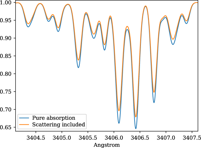
Figure 2. Synthetic spectra for star HP1-2115 with (Teff = 4530, log g = 2.0,[Fe/H] = −1.0, v t = 1.45), illustrating the change in the continuum, with both absorption and scattering (blue spectrum), and considering pure absorption (orange spectrum).
3.2.5. Atomic line lists
Atomic line lists can be converted from Vald3 (extended format) (Piskunov et al. Reference Piskunov, Kupka, Ryabchikova, Weiss and Jeffery1995, Ryabchikova et al. Reference Ryabchikova, Piskunov, Kurucz, Stempels, Heiter, Pakhomov and Barklem2015) lists of atomic lines. The VALD atomic line list started with basically the list by Kurúcz (Reference Kurúcz1995, Reference Kurúcz2017), with progressive implementation of improvements coming from different sources. The default atomic line list in the range 3 000–10 000 Å is from VALD, where the collisional broadening is obtained by adopting a general formula for the van der Waals broadening (e.g. Gray Reference Gray2005). Better broadening constant values can be obtained through the code from Anstee & O’Mara (Reference Anstee and O’Mara1995), Barklem & O’Mara (Reference Barklem and O’Mara1997), Barklem, Anstee, & O’Mara (Reference Barklem, Anstee and O’Mara1998), and Barklem, Piskunov, & O’Mara (Reference Barklem, Piskunov and O’Mara2000) (this series of papers is referred to hereafter as ABO) for neutral lines.
The list of lines in the NIR adopted is from Meléndez & Barbuy (Reference Meléndez and Barbuy1999). An up-to-date such line list is given by Shetrone et al. (Reference Shetrone2015).
Other options of line lists are available, in particular, our own list that includes damping parameters from ABO for most lines in the visible region, and lists of hyperfine structure for several elements, that can be obtained by contacting the authors.
3.2.6. Molecular line lists
The list of molecules, their system, wavelength coverage, number of vibrational transitions (v′, v″), the constants dissociation potential D 0 (eV), and the electronic oscillator strength f el, that is related to the transition moment Re, with corresponding references are given in Table 1. This list of molecular lines is included in the code package, in file molecules.dat.
Table 1. Molecular lines included in Pfant and respective sources of data: line lists, dissociation potential D o, electronic oscillator strength f el
References: (1) Balfour & Cartwright (Reference Balfour and Cartwright1976); (2) Phillips & Davis (Reference Phillips and Davis1968); (3) Kurúcz (Reference Kurúcz1993a); (4) Davis & Phillips (Reference Davis and Phillips1963); (5) Luque & Crosley (Reference Luque and Crosley1999); (6) Goorvitch (Reference Goorvitch1994); (7) Fernando et al. (Reference Fernando, Bernath, Hodges and Masseron2018); (8) Abrams et al. (Reference Abrams, Davis, Rao, Engleman and Brault1994); (9) Goldman et al. (Reference Goldman, Schoenfeld, Goorvitch, Chackerian, Dothe, Mélen, Abrams and Selby1998); (10) Phillips et al. (Reference Phillips, Davis, Lindgren and Balfour1987); (11) Alvarez & Plez (Reference Alvarez and Plez1998); (12) Jorgensen (Reference Jorgensen1994); (13) Plez (Reference Plez1998); (14) Huber & Herzberg (Reference Huber and Herzberg1979); (15) Pradhan, Partridge, & Bauschlicher (Reference Pradhan, Partridge and Bauschlicher1994); (16) Schultz & Armentrout (Reference Schultz and Armentrout1991); (17) Henneker & Popkie (Reference Henneker and Popkie1971); (18) Kirby, Saxon, & Liu (Reference Kirby, Saxon and Liu1979); (19) Duric, Erman, & Larsson (Reference Duric, Erman and Larsson1978); (20) Bauschlicher, Langhoff, & Taylor (Reference Bauschlicher, Langhoff and Taylor1988); (21) Brzozowski et al. (Reference Brzozowski, Bunker, Elander and Erman1976); (22) Grevesse & Sauval (Reference Grevesse and Sauval1973); (23) Lambert (Reference Lambert1978); (24) Goldman et al. (Reference Goldman, Schoenfeld, Goorvitch, Chackerian, Dothe, Mélen, Abrams and Selby1998); (25) Schiavon et al. (Reference Schiavon, Barbuy and Singh1997).
a 12CH + 13CH.
In the near-ultraviolet and visible, the line lists from KurúczFootnote b were adopted (and transformed to our format) for OH and CN blue. CH lines are from Luque & Crosley (Reference Luque and Crosley1999). MgH lines are from Balfour & Cartwright (Reference Balfour and Cartwright1976). The NH blue lines are adopted from the recent line lists by Fernando et al. (Reference Fernando, Bernath, Hodges and Masseron2018). The CN red and C2 Swan lines are from C2 laboratory line lists by Phillips & Davis (Reference Phillips and Davis1968), and CN A 2Π−X 2Σ red line lists by Davis & Phillips (Reference Davis and Phillips1963). TiO line lists are from Alvarez & Plez (Reference Alvarez and Plez1998), Plez (Reference Plez1998), and Jorgensen (Reference Jorgensen1994)—see Schiavon & Barbuy (Reference Schiavon and Barbuy1999). FeH line lists are from Phillips et al. (Reference Phillips, Davis, Lindgren and Balfour1987), and constants are described in Schiavon, Barbuy, & Singh (Reference Schiavon, Barbuy and Singh1997)..
Note that the MgH, CN red, C2, and FeH adopted correspond to laboratory measurements, differently to line lists available in most of the other codes.
In the NIR, the CO X 1Σ lines are from Goorvitch (Reference Goorvitch1994). The OH X2Π lines were made available by S. P. Davis that were originally from Abrams et al. (Reference Abrams, Davis, Rao, Engleman and Brault1994) with a few theoretical lines from Goldman et al. (Reference Goldman, Schoenfeld, Goorvitch, Chackerian, Dothe, Mélen, Abrams and Selby1998)—see Meléndez & Barbuy (Reference Meléndez and Barbuy1999) and Meléndez, Barbuy, & Spite (Reference Meléndez, Barbuy and Spite2001).
Next we describe the structure of the Pfant molecular line lists files, which are hierarchically organised as follows:
1. for each molecular system: constants including the electronic oscillator strength f el and dissociation constant D 0
2. for each (v′, v″) transition in each molecular system: qv ′v ″, G 0(v), Bv, Dv
3. for each molecular line in each (v′, v″) transition: λ 0J ′J ″, J″,
${({{\mathscr S}_{{\rm{n}}orm}})_{J'J''}}$, where (using Equation (17))

 $${({{\mathscr S}_{{\rm{n}}orm}})_{J'J''}} = \frac {{{\mathscr S}_{J'J''}}} {(2 - {\delta _{0,\Lambda ' + \Lambda ''}})(2S + 1)(2J + 1)},$$(39)
so that (sum for all branches, fixed J)
 $$\sum {({{\mathscr S}_{{\rm{n}}orm}})_{J'J''}} = 1.$$(40)
G 0(v), Bv, Dv are calculated as follows:
 $$\begin{eqnarray*} &&\kern8.7ptB_{v} = B_{\rm e} - \alpha_{\rm e} (v+0.5), \\[3pt] &&\kern7.5ptD_{v} = (D_{\rm e} + \beta_{\rm e} (v+0.5)) \times 10^6, \\[3pt] &&G(0) = \omega_{\rm e} / 2.0 - \omega_{\rm e}x_{\rm e} / 4.0 + \omega_{\rm e}y_{\rm e} / 8.0, \\[3pt] &&\kern0.2ptG(v) = \omega_{\rm e} (v+0.5) - \omega_{\rm e}x_{\rm e}(v+0.5)^2 + \omega_{\rm e}y_{\rm e}(v+0.5)^3, \\[3pt] &&\kern-3.3ptG_0(v) = G(v) - G(0) \end{eqnarray*}$$
3.2.7. Extending the molecular line list
Several databases present updated line lists. Some of the most well known are described below:
Bertrand Plez’s websiteFootnote c links to a directory of line lists in various formats. A constant update in line lists such as CH (Masseron et al. Reference Masseron2014) and NH (Fernando et al. Reference Fernando, Bernath, Hodges and Masseron2018) carried out within Turbospectrum makes it extremely important to be able to implement these new data in other codes (and our own) by converting the formats from each other—see below and Section 3.3.1.
The Robert L. Kurúcz websiteFootnote d compiles several line lists converted to a standardised format (herein referred to as the ‘Kurúcz format’).
The High Resolution Transmission (HITRAN) brings molecular line lists, with description updated in Rothman et al. (Reference Rothman2013).
As concerns complete line lists, the drawback is that they can reach millions of theoretical lines, with most of them being weak. The situation is similar to the millions of weak atomic lines (Kurúcz Reference Kurúcz1995). It is not our intent here to cover all these weak lines. This is accomplished, for example, by Tennyson & Yurchenko (Reference Tennyson and Yurchenko2012), where laboratory and earlier calculations of molecular lines are completed by ab inition quantum mechanical treatment. Their line lists are presented in a standardised format using Einstein coefficients in the Exomol database.Footnote e
The webpage by Peter BernathFootnote f contains a database on papers regarding a series of molecules.
The webpage by Jeremy BaileyFootnote g brings line lists, links to other databases, and software tools.
The Virtual Atomic and Molecular Data Centre Consortium—VAMDCFootnote h gives access to 36 inter-connected atomic and molecular databases (Dubernet et al. Reference Dubernet, Zwölf, Moreau and Ba2016).
Given all the different formats of the line lists available, line list conversion codes are valuable resources, as they allow for validations of synthesis codes and exchanges among research groups. We implemented a tool to convert molecular line lists from the Kurúcz formats (old and new) and also from the Turbospectrum/Bsyn format, to the Pfant format, as described in Section 3.3.1. Other conversion paths are planned.
3.2.8. Output spectra
The code pfant generates three output files corresponding to the continuum, un-normalised flux, and normalised flux. As usual, the normalised flux is fluxnorm(λ) = fluxun-normalised(λ)/fluxcontinuum(λ).
The code nulbad takes pfant output spectra, convolves it with a Gaussian profile (GP), and generates a file that, by default, contains the FWHM (full width at half maximum, given in Å) of the Gaussian profile in its name. This is a two-column text file with the wavelength (Å) and flux.
3.3. Python interface and tools
With package pyfant (http://trevisanj.github.io/pyfant), one can write scripts that use Pfant spectral synthesis in the core of more complex tasks (e.g. automatic determination of stellar parameters) in the Python language. The pyfant package application programming interface (API) includes resources to run Pfant spectral synthesis in series and in parallel, and to load, filter, transform, save, and visualise relevant data files.
In addition, pyfant contains a series of command-line and graphical tools (command-line and graphical interfaces) to perform various tasks, including a scraper of molecular constants from the NIST chemistry web book, an atomic lines converter from Vald3 to Pfant format, a molecular line list converter to the Pfant format, a tool to create grids of MARCS models, an editor for atomic lines, and an editor for molecular lines. A complete list of tools is obtained by running script programs.py in the computer terminal.
3.3.1. Conversion of molecular line lists
A systematic method to convert molecular line lists to the Pfant format was implemented. Conversion can be carried out with very little user interaction, provided that:
Diatomic molecular constants are available in the NIST chemistry web book for the particular molecular systems of choice.Footnote i
The input line list format contains sufficient information to determine the branch of each line.
In this section we discuss some particularities with the conversions of the Kurúcz and Turbospectrum line lists. For the Kurúcz format, the branch can be determined from the tabulated J′, J″, spin′, and spin″ as follows:
“P” if J″ > J′;
“Q” if J″ = J′;
“R” if J″ < J′.
And in more detail if it is ‘P1’, ‘P2’, ‘P3’, etc. is indicated by the spin of the lower state and upper states. If spin″ = spin′, the branch is ‘(P/Q/R)(spin)’, If spin″ ≠ spin, the branch is ‘(P/Q/R)(spin′)(spin″)’.
Turbospectrum line lists already contain the branch given as a string, for example, ‘R23’.
The branch is used to determine the specific formula from Kovács (Reference Kovács1969) that will be used to calculate  ${{\mathscr S}_{J'J''}}$. This choice of formula is a detailed procedure and depends on:
the multiplicity of the transition (singlet, doublet, triplet);
the sign and value of ΔΛ = Λ′ − Λ″;
the sign of A; and
the branch.
The Franck–Condon factors qv ′v ″ (Equation 16) are computed with the code for transition probabilities of molecular transitions by Jarmain & McCallum (Reference Jarmain and McCallum1970) (TRAPRB). The qv ′v ″ factors are dependent on the system and the vibrational levels and have almost no dependence on rotational constants (Singh & de Almeida Reference Singh and de Almeida1982).
The procedure described above to convert molecular line lists is coded as part of the pyfant API and is available as a graphical application named convmol.py. This application interfaces with the NIST chemistry web book to get the diatomic molecular constants A, B e, α e, β e, ω e, ω ex e, and ω ey e (these can be later tuned if necessary), and interfaces with code TRAPRB to calculate qv ′v ″.
3.4. Comparison with stellar spectra and code Turbospectrum
A validation of the code Pfant is presented here, with the comparison of the CN blue B 2Σ – X 2Σ (v′ = 0,v″ = 0) bandhead (Figure 3), the CH A 2Δ – X 2Π (0,0) G-bandhead (Figure 4), and the NH A 3Π−X 3Σ (0,0) bandhead (Figure 5) of the spectra resulting from the calculations with Pfant, Turbospectrum, and the observed solar spectrum (Kurúcz et al. Reference Kurúcz, Furenlid, Brault and Testerman1984).
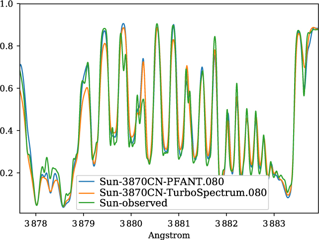
Figure 3. Synthetic and observed spectra of the the Sun, in the region of the CN B 2Σ−X 2Σ (0,0) bandhead: observed spectrum (green); synthetic spectra with Turbospectrum (orange), and with Pfant (blue).
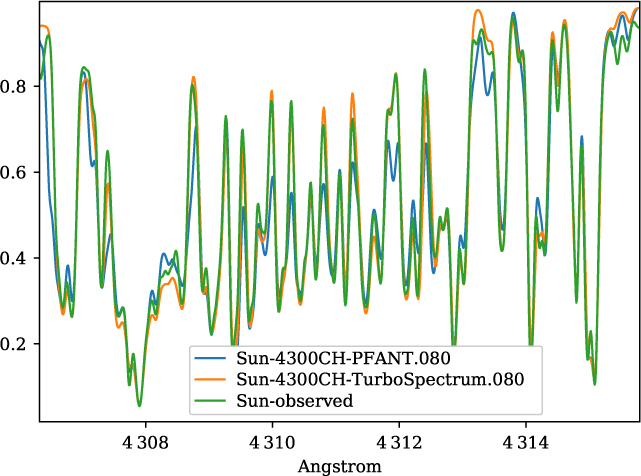
Figure 4. Synthetic and observed spectra of the the Sun, in the region of the CH A 2Δ – X 2Π (0,0) G-bandhead: observed spectrum (green); synthetic spectra with Turbospectrum (orange), and with Pfant (blue).
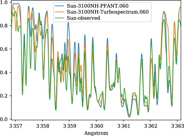
Figure 5. Synthetic and observed spectra of the the Sun, in the region of the NH A 3Π – X 3Σ (0,0) bandhead: observed spectrum (green); synthetic spectra with Turbospectrum (orange), and with Pfant (blue).
4. Summary
We present the description of calculation of diatomic molecular lines, given that this task is not straightforward. Molecular line intensities in the literature are given in either of the two formats: the Einstein A constant, related to the oscillator strength (see Section 2), or else the inclusion of all the ingredients that build together the oscillator strength.
We present a description of a new updated online version of the code for spectrum synthesis Pfant, together with many accessory tools and documentation. We describe the molecular line lists adopted, recalling that they need constant updating and implementation of new molecules. One example of an important update is the recent line list for NH (Fernando et al. Reference Fernando, Bernath, Hodges and Masseron2018). The package includes codes for conversion of molecular line lists to the Pfant format, in particular so far from Kurúcz’s and Plez’s line lists. The atomic line list is also in constant improvement, both from the Vald3 database, as our own line list (available upon request).
Acknowledgements
We are grateful to the referee for constructive comments that helped improving the code and the paper. We thank J. Meléndez and R. Smiljanic for useful comments on a previous version of the manuscript. BB and AA acknowledge grants from CAPES—Finance code 001, CNPq and FAPESP. JT acknowledges the TT-5 FAPESP fellowships 2014/25987-5 and 2016/00777-3.


