


Logit and probit models have become a staple in quantitative political and social science—nearly as common as linear regression (Krueger and Lewis-Beck, Reference Krueger and Lewis-Beck2008). And although the usual maximum likelihood (ML) estimates of logit and probit model coefficients have excellent large-sample properties, these estimates behave quite poorly in small samples. Because the researcher cannot always collect more data, this raises an important question: How can a researcher obtain reasonable estimates of logit and probit model coefficients using only a small sample? In this paper, we remind political scientists that Firth's (Reference Firth1993) penalized maximum likelihood (PML) estimator greatly reduces the small-sample bias of ML estimates of logit model coefficients. We show that the PML estimator nearly eliminates the bias, which can be substantial. But even more importantly, the PML estimator dramatically reduces the variance of the ML estimator. Of course, the inflated bias and variance of the ML estimator lead to a larger overall mean-squared error (MSE). Using an example from published research (George and Epstein, Reference George and Epstein1992), we illustrate the differences in the ML and PML estimators. Moreover, we offer Monte Carlo evidence that the PML estimator offers a substantial improvement in small samples (e.g., 100 observations) and noticeable improvement even in large samples (e.g., 1000 observations).
1. The big problem with small samples
When working with a binary outcome $y_i$ , the researcher typically models probability of an event, so that

where $y$ represents a vector of binary outcomes, $X$
 represents a matrix of explanatory variables and a constant, $\beta$
 represents a vector of model coefficients, and $g^{-1}$
 represents some inverse-link function that maps ${\opf R}$
 into $[ 0,\; 1]$
 . When $g^{-1}$
 represents the inverse-logit function $\text {logit}^{-1}( \alpha ) = {1}/( {1 + {\rm e}^{-\alpha }) }$
 or the cumulative normal distribution function $\Phi ( \alpha ) = \int _{-\infty }^{\alpha } ( {1}/{\sqrt {2\pi }}) {\rm e}^{-( {x^{2}}/{2}) }dx$
 , then we refer to Equation 1 as a logit or probit model, respectively. To simplify the exposition, we focus on logit models because the canonical logit link function induces nicer theoretical properties (McCullagh and Nelder, Reference McCullagh and Nelder1989: 31–32). In practice, though, Kosmidis and Firth (Reference Kosmidis and Firth2009) show that the ideas we discuss apply equally well to probit models.
To develop the ML estimator of the logit model, we can derive the likelihood function

and, as usual, take the natural logarithm of both sides to obtain the log-likelihood function

The researcher can obtain the ML estimate $\hat {\beta }^{\rm mle}$ by finding the vector $\beta$
 that maximizes $\log L$
 given $y$
 and $X$
 (King, Reference King1998).Footnote 1
The ML estimator has excellent properties in large samples. It is asymptotically unbiased, so that $E( \hat {\beta }^{\rm mle}) \approx \beta ^{\rm true}$ when the sample is large (Casella and Berger, Reference Casella and Berger2002: 470; Wooldridge, Reference Wooldridge2002: 391–395). It is also asymptotically efficient, so that the asymptotic variance of the ML estimate obtains the Cramer–Rao lower bound (Casella and Berger, Reference Casella and Berger2002: 472, 516; Greene, Reference Greene2012: 513–523). For small samples, though, the ML estimator of logit model coefficients does not work well—the ML estimates have substantial bias away from zero (Long, Reference Long1997: 53–54).
Long (Reference Long1997: 54) offers a rough heuristic about appropriate sample sizes: “It is risky to use ML with samples smaller than 100, while samples larger than 500 seem adequate.”Footnote 2 This presents the researcher with a problem: When dealing with small samples, how can she obtain reasonable estimates of logit model coefficients?
2. An easy solution for the big problem
The statistics literature offers a simple solution to the problem of bias. Firth (Reference Firth1993) suggests penalizing the usual likelihood function $L( \beta \vert y)$ by a factor equal to the square root of the determinant of the information matrix $\vert I( \beta ) \vert ^{{1}/{2}}$
 , which produces a “penalized” likelihood function $L^{\ast }( \beta \vert y) = L( \beta \vert y) \vert I( \beta ) \vert ^{{1}/{2}}$
 (see also Kosmidis and Firth Reference Kosmidis and Firth2009; Kosmidis Reference Kosmidis2014).Footnote 3 It turns out that this penalty is equivalent to Jeffreys’ (Reference Jeffreys1946) prior for the logit model (Firth Reference Firth1993; Poirier Reference Poirier1994). We take the natural logarithm of both sides to obtain the penalized log-likelihood function:

Then the researcher can find the PML estimate $\hat {\beta }^{{\rm pmle}}$ by finding the vector $\beta$
 that maximizes $\log L^{\ast }$
 .Footnote 4$^{, }$
 Footnote 5
Zorn (Reference Zorn2005) suggests PML for solving the problem of separation, but the broader and more important application to small sample problems seems to remain under-appreciated in political science.Footnote 6 Most importantly, though, we show that the small-sample bias should be of secondary concern to the small-sample variance of ML. Fortunately, PML reduces both the bias and the variance of the ML estimates of logit model coefficients.
A researcher can implement PML as easily as ML, but PML estimates of logit model coefficients have a smaller bias (Firth, Reference Firth1993) and a smaller variance (Copas, Reference Copas1988; Kosmidis Reference Kosmidis2007: 49).Footnote 7 This is important. When choosing among estimators, researchers often face a tradeoff between bias and variance (Hastie et al., Reference Hastie, Tibshirani and Friedman2013: 37–38), but there is no bias-variance tradeoff between ML and PML estimators. The PML estimator exhibits both lower bias and lower variance.
Two concepts from statistical theory illuminate the improvement offered by the PML estimator over the ML estimator. Suppose two estimators $A$ and $B$
 , with a quadratic loss function so that the risk functions $R^{A}$
 and $R^{B}$
 (i.e., the expected loss) correspond to the MSE. If $R^{A} \leq R^{B}$
 for all parameter values and the inequality holds strictly for at least some parameter values, then we can refer to estimator $B$
 as inadmissible and say that estimator $A$
 dominates estimator $B$
 (Leonard and Hsu, Reference Leonard and Hsu1999: 143–146; DeGroot and Schervish, Reference DeGroot and Schervish2012: 458). Now suppose a quadratic loss function for the logit model coefficients, such that $R^{\rm mle} = E[ ( \hat {\beta }^{\rm mle} - \beta ^{\rm true}) ^{2}]$
 and $R^{{\rm pmle}} = E[ ( \hat {\beta }^{{\rm pmle}} - \beta ^{\rm true}) ^{2}]$
 . In this case, the inequality holds strictly for all $\beta ^{\rm true}$
 so that $R^{{\rm pmle}} < R^{\rm mle}$
 . For logit models, then, we can describe the ML estimator as inadmissible and say that the PML estimator dominates the ML estimator.
The intuition of the bias reduction is subtle. First, consider the source of the bias, illustrated in Figure 1. Calculate the score function $s$ as the gradient (or first-derivative) of the log-likelihood with respect to $\beta$
 so that $s( y,\; \beta ) = \nabla \log L( \beta \vert y)$
 . Note that solving $s( y,\; \hat {\beta }^{\rm mle}) = 0$
 is equivalent to finding $\hat {\beta }^{\rm mle}$
 that maximizes $\log L( \beta \vert y)$
 . Now recall that at the true parameter vector $\beta ^{\rm true}$
 , the expected value of the score function is zero so that $E[ s( y,\; \beta ^{\rm true}) ] = 0$
 (Greene, Reference Greene2012: 517). By the law of total probability, this implies that

which is highlighted by (i) in Figure 1.
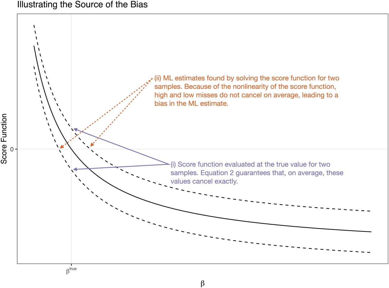
Figure 1. Illustration of the source of the bias using the score functions for two hypothetical samples shown with dashed lines. Notice that, when evaluated at $\beta ^{\rm true}$ , the score functions cancel on average (Equation 2). However, the nonlinearity of the score function pushes the ML estimate of the high miss (top line) relatively further from the true value. On the other hand, the nonlinearity of the score function pulls the ML estimate of the low miss (bottom line) relatively closer.
However, if the score function $s$ is decreasing and curved in the area around $\beta ^{\rm true}_j$
 so that $s''_j = {\partial ^{2} s( y,\; \beta ) }/{\partial ^{2} \beta _j} > 0$
 (see Figure 1), then a high miss $s( y,\; \beta ^{\rm true}) > 0$
 (top dashed line in Figure 1) implies an estimate well above the true value, so that $\hat {\beta }^{\rm mle} \gg \beta ^{\rm true}$
 , and a low miss (bottom dashed line in Figure 1) $s( y,\; \beta ^{\rm true}) < 0$
 implies an estimate only slightly below the true value, so that $\hat {\beta }^{\rm mle} < \beta ^{\rm true}$
 . In effect, the curved (convex) score function pulls low misses closer the true value and pushes high misses even further from the true value. This dynamic, which is highlighted by (ii) in Figure 1, implies that low misses and high misses do not cancel and that the ML estimate is too large on average. A similar logic applies for $s''_j < 0$
 . Therefore, due to the curvature in the score function $s$
 , the high and low misses of $\hat {\beta }^{\rm mle}$
 do not cancel out, so that $E( \hat {\beta }^{\rm mle}_j) > \beta ^{\rm true}_j$
 when $s''_j > 0$
 and $E( \hat {\beta }^{\rm mle}) < \beta ^{\rm true}_j$
 when $s''_j < 0$
 . Cox and Snell (Reference Cox and Snell1968: 251–252) derive a formal statement of this bias of order $n^{-1}$
 , which we denote as $\text {bias}_{n^{-1}}( \beta ^{\rm true})$
 .
.
Now consider the bias reduction strategy. At first glance, one may simply decide to subtract $\text {bias}_{n^{-1}}( \beta ^{\rm true})$ from the estimate $\hat {\beta }^{\rm mle}$
 . However, note that the bias depends on the true parameter. Because researchers do not know the true parameter, this is not the most effective strategy.Footnote 8 However, Firth (Reference Firth1993) suggests modifying the score function, so that $s^{\ast }( y,\; \beta ) = s( y,\; \beta ) - \gamma ( \beta )$
 , where $\gamma$
 shifts the score function upward or downward. Firth (Reference Firth1993) shows that one good choice of $\gamma$
 takes $\gamma _j = ( {1}/{2}) \text {trace} [ I^{-1} ( {\partial I}/{\partial \beta _j}) ] = ( {\partial }/{\partial \beta _j}) ( \log \vert I( \beta ) \vert )$
 . Integrating, we can see that solving $s^{\ast }( y,\; \hat {\beta }^{{\rm pmle}}) = 0$
 is equivalent to finding $\hat {\beta }^{{\rm pmle}}$
 that maximizes $\log L^{\ast }( \beta \vert y)$
 with respect to $\beta$
 .
.
The intuition of the variance reduction is straightforward. Because PML shrinks the ML estimates toward zero, the PML estimates must have a smaller variance than the ML estimates. If we imagine the PML estimates as trapped between zero and the ML estimates, then the PML estimates must be less variable.
What can we say about the relative performance of the ML and PML estimators? Theoretically, we can say that the PML estimator dominates the ML estimator because the PML estimator has lower bias and variance regardless of the sample size. That is, the PML estimator always outperforms the ML estimator, and least in terms of the bias, variance, and MSE. However, both estimators are asymptotically unbiased and efficient, so the difference between the two estimators becomes negligible as the sample size grows large. In small samples, though, Monte Carlo simulations show substantial improvements that should appeal to substantive researchers.
3. The big improvements from an easy solution
To show that the size of reductions in bias, variance, and MSE should draw the attention of substantive researchers, we conduct a Monte Carlo simulation comparing the sampling distributions of the ML and PML estimates. These simulations demonstrate three features of the ML and PML estimators:
(1) In small samples, the ML estimator exhibits a large bias. The PML estimator is nearly unbiased, regardless of sample size.
(2) In small samples, the variance of the ML estimator is much larger than the variance of the PML estimator.
(3) The increased bias and variance of the ML estimator implies that the PML estimator also has a smaller MSE. Importantly, though, the variance makes a much greater contribution to the MSE than the bias.
In our simulation, the true data generating process corresponds to $\Pr ( y_i = 1) = {1}/( {1 + {\rm e}^{-X_i \beta }) }$ , where $i \in 1,\; 2,\; \ldots ,\; n$
 and $X \beta = \beta _{\rm cons} + 0.5 x_1 + \sum _{j = 2}^{k} 0.2 x_j$
 , and we focus on the coefficient for $x_1$
 as the coefficient of interest. We draw each fixed $x_j$
 independently from a normal distribution with mean of zero and standard deviation of one and vary the sample size $N$
 from 30 to 210, the number of explanatory variables $k$
 from 3 to 6 to 9, and the intercept $\beta _{\rm cons}$
 from $-1$
 to $-0.5$
 to 0 (which, in turn, varies the proportion of events $P_{\rm cons}$
 from about 0.28 to 0.38 to 0.50).Footnote 9
Each parameter in our simulation varies the amount of information in the data set. The biostatistics literature uses the number of events per explanatory variable $( {1}/{k}) \sum y_i$ as a measure of the information in the data set (e.g., Peduzzi et al., Reference Peduzzi, Concato, Kemper, Holford and Feinstein1996; Vittinghoff and McCulloch, Reference Vittinghoff and McCulloch2007), and each parameter of our simulation varies this quantity, where $( {N \times P_{\rm cons}}) /{k} \approx ( {1}/{k}) \sum y_i$
 . For each combination of the simulation parameters, we draw 50,000 data sets and use each data set to estimate the logit model coefficients using ML and PML. To avoid an unfair comparison, we exclude the ML estimates where separation occurs (Zorn, Reference Zorn2005). We keep all the PML estimates. Replacing the ML estimates with the PML estimates when separation occurs dampens the difference between the estimators and keeping all the ML estimates exaggerates the differences. From these estimates, we compute the percent bias and variance of the ML and PML estimators, as well as the MSE inflation of the ML estimator compared to the PML estimator.
3.1 Bias
We calculate the percent bias $= 100\% \times ( {E( \hat {\beta }) }/{\beta ^{\rm true}} - 1 )$ as the intercept $\beta _{\rm cons}$
 , the number of explanatory variables $k$
 , and the sample size $N$
 vary. Figure 2 shows the results. The sample size varies across the horizontal-axis of each plot and each panel shows a distinct combination of intercept and number of variables in the model. Across the range of the parameters of our sample, the bias of the ML estimate varies from about 122 percent ($\beta _{\rm cons} = -0.5$
 , $k = 9$
 , and $N = 30$
 ) to around 3 percent ($\beta _{\rm cons} = -1$
 , $k = 3$
 , and $N = 210$
 ). The bias in the PML estimate, on the other hand, is much smaller. For the worst-case scenario ($\beta _{\rm cons} = -0.5$
 , $k = 9$
 , and $N = 30$
 ), the ML estimate has an upward bias of about 122 percent, while the PML estimate has an upward bias of only about 12 percent.Footnote 10

Figure 2. Substantial bias of $\hat {\beta }^{\rm mle}$ and the near unbiasedness of $\hat {\beta }^{{\rm pmle}}$
 .
.
3.2 Variance
In many cases, estimators tradeoff bias and variance, but the PML estimator reduces both. In addition to nearly eliminating the bias, Figure 3 shows that the PML estimator also substantially reduces the variance, especially for the smaller sample sizes. For $\beta _{\rm cons} = -1$ and $N = 30$
 , the variance of the ML estimator is about 99, 178, and 436 percent larger than the PML estimator for three, six, and nine variables, respectively. Doubling the sample size to $N = 60$
 , the variance remains about 25, 58, and 117 percent larger, respectively. Even for a larger sample of $N = 210$
 , the variance of the ML estimator is about 6, 10, and 14 percent larger than the PML estimator.Footnote 11

Figure 3. Smaller variance of $\hat {\beta }^{{\rm pmle}}$ compared to $\hat {\beta }^{\rm mle}$
 .
.
3.3 Mean-squared error
However, neither the bias nor the variance serves as a complete summary of the performance of an estimator. The MSE, though, combines the bias and variance into an overall measure of the accuracy, where

Since the bias and the variance of the ML estimator exceeds the bias and variance the PML estimator, the ML estimator must have a larger MSE, so that ${\rm MSE}( \hat {\beta }^{\rm mle}) - {\rm MSE}( \hat {\beta }^{{\rm pmle}}) > 0$ .
.
We care about the magnitude of this difference, though, not the sign. To summarize the magnitude, we compute the percent increase in the MSE of the ML estimator compared to the PML estimator. We refer to this quantity as the “MSE inflation,” where

An MSE inflation of zero indicates that the ML and PML estimators perform equally well, but because the PML estimator dominates the ML estimator, the MSE inflation is strictly greater than zero. Figure 4 shows the MSE inflation for each combination of the parameter simulations on the log$_{10}$ scale. Notice that for the worst-case scenario ($\beta _{\rm cons} = -1$
 , $k = 9$
 , and $N = 30$
 ), the MSE of the ML estimates is about 721 percent larger than the MSE of the PML estimates. The MSE inflation only barely drops below 10 percent for the most information-rich parameter combinations (e.g., $\beta _{\rm cons} = 0$
 , $k = 3$
 , and $N = 210$
 ). The MSE inflation exceeds 100 percent for about 11 percent of the simulation parameter combinations, 50 percent for about 21 percent of the combinations, and 25 percent for about 45 percent of the combinations. These large sacrifices in MSE should command the attention of researchers working with binary outcomes and small data sets.

Figure 4. Percent increase in the MSE of $\hat {\beta }^{\rm mle}$ compared to $\hat {\beta }^{{\rm pmle}}$
 .
.
However, the larger bias and variance of the ML estimator do not contribute equally to the MSE inflation. Substituting Equation 3 into Equation 4 for ${\rm MSE}( {\hat \beta }^{\rm mle})$ and ${\rm MSE}( {\hat \beta }^{{\rm pmle}})$
 and rearranging, we obtain

which additively separates the contribution of the bias and variance to the MSE inflation. If we wanted, we could simply plug in the simulation estimates of the bias and variance of each estimator to obtain the contribution of each. But notice that we can easily compare the relative contributions of the bias and variance using the ratio

Figure 5 shows the relative contribution of the variance. Values less than 1 indicate that the bias makes a greater contribution and values greater than 1 indicate that the variance makes a greater contribution. In each case, the relative contribution of the variance is much larger than 1. For $N = 30$ , the contribution of the variance is between 4 and 17 times larger than the contribution of the bias. For $N = 210$
 , the contribution of the variance is between 27 and 166 times larger than the contribution of the bias. In spite of the attention paid to the small sample bias in ML estimates of logit model coefficients, the small sample variance is a more important problem to address, at least in terms of the accuracy of the estimator. Fortunately, the PML estimator greatly reduces the bias and variance, resulting in a much smaller MSE, especially for small samples.

Figure 5. Relative contribution of the variance and bias to the MSE inflation. The relative contribution is defined in Equation 5.
These simulation results show that the bias, variance, and MSE of the ML estimates of logit model coefficients are not trivial in small samples. Researchers cannot safely ignore these problems. Fortunately, researchers can implement the PML estimator with little to no added effort and obtain substantial improvements over the usual ML estimator. And these improvements are not limited to Monte Carlo studies. In the example application that follows, we show that the PML estimator leads to substantial reductions in the magnitude of the coefficient estimates and in the width of the confidence intervals.
4. The substantive importance of the big improvements
To illustrate the substantive importance of using the PML estimator, we reanalyze a portion of the statistical analysis in George and Epstein (Reference George and Epstein1992).Footnote 12 We re-estimate the integrated model of US Supreme Court decisions developed by George and Epstein (Reference George and Epstein1992) and find substantial differences in the ML and PML coefficient estimates and the confidence intervals.
George and Epstein (Reference George and Epstein1992) combine the legal and extralegal models of Court decision-making in order to overcome the complementary idiosyncratic shortcomings of each. The legal model posits stare decisis, or the rule of law, as the key determinant of future decisions, while the extralegal model takes a behavioralist approach containing an array of sociological, psychological, and political factors.
The authors model the probability of a conservative decision in favor of the death penalty as a function of a variety of legal and extralegal factors. George and Epstein use a small sample of 64 Court decisions involving capital punishment from 1971 to 1988. The data set has only 29 events (i.e., conservative decisions). They originally use the ML estimator, and we reproduce their estimates exactly. For comparison, we also estimate the model with the PML estimator that we recommend. Figure 6 shows the coefficient estimates for each method. In all cases, the PML estimate is smaller than the ML estimate. Each coefficient decreases by at least 25 percent with three decreasing by more than 40 percent. Additionally, the PML estimator substantially reduces the width of all the confidence intervals. Three of the 11 coefficients lose statistical significance.

Figure 6. Coefficients for a logit model estimating US Supreme Court Decisions by both ML and PML.
Because we do not know the true model, we cannot know which of these sets of coefficients is better. However, we can use out-of-sample prediction to help adjudicate between these two methods. We use leave-one-out cross-validation and summarize the prediction errors using Brier and log scores, for which smaller values indicate better predictive ability.Footnote 13 The ML estimates produce a Brier score of 0.17, and the PML estimates lower the Brier score by 7 percent to 0.16. Similarly, the ML estimates produce a log score of 0.89, while the PML estimates lower the log score by 41 percent to 0.53. The PML estimates outperform the ML estimates for both approaches to scoring, and this provides good evidence that the PML estimates better capture the data generating process.
Because we estimate a logit model, we are likely more interested in the functions of the coefficients rather than the coefficients themselves (King et al., Reference King, Tomz and Wittenberg2000). For an example, we take George and Epstein's integrated model of Court decisions and calculate a first difference and risk ratio as the repeat-player status of the state varies, setting all other explanatory variables at their sample medians. George and Epstein hypothesize that repeat players have greater expertise and are more likely to win the case. Figure 7 shows the estimates of the quantities of interest.

Figure 7. Quantities of interest for the effect of the solicitor general filing a brief amicus curiae on the probability of a decision in favor of capital punishment.
The PML estimator pools the estimated probabilities toward one-half. When the state is not a repeat player, the PML estimates suggest a 17 percent chance of a conservative decision while ML estimates suggest only a 6 percent chance. However, when the state is a repeat player, the PML estimates suggest that the Court has a 69 percent chance of a conservative decision compared to the 68 percent chance suggested by ML. Thus, PML also provides smaller effect sizes for both the first difference and the risk ratio. PML decreases the estimated first difference by 17 percent from 0.63 to 0.52 and the risk ratio by 67 percent from 12.3 to 4.0.
This example application clearly highlights the differences between the ML and PML estimators. The PML estimator shrinks the coefficient estimates and confidence intervals substantially. Theoretically, we know that these estimates have a smaller bias, variance, and MSE. Practically, though, this shrinkage manifests in smaller coefficient estimates, smaller confidence intervals, and better out-of-sample predictions. And these improvements come at almost no cost to researchers. The PML estimator is nearly trivial to implement but dominates the ML estimator—the PML estimator always has lower bias, lower variance, and lower MSE.
5. Recommendations to substantive researchers
Throughout this paper, we emphasize one key point—when using small samples to estimate logit and probit models, the PML estimator offers a substantial improvement over the usual ML estimator. But what actions should substantive researchers take in response to our methodological point? In particular, at what sample sizes should researchers consider switching from the ML estimator to the PML estimator?
5.1 Concrete advice about sample sizes
Prior research suggests two rules of thumb about sample sizes. First, Peduzzi et al. (Reference Peduzzi, Concato, Kemper, Holford and Feinstein1996) recommend about ten events per explanatory variable, although Vittinghoff and McCulloch (Reference Vittinghoff and McCulloch2007) suggest relaxing this rule. Second, Long (Reference Long1997: 54) suggests that “it is risky to use ML with samples smaller than 100, while samples larger than 500 seem adequate.” In both of these cases, the alternative to a logit or probit model seems to be no regression at all. Here, though, we present the PML estimator as an alternative, so we have room to make more conservative recommendations.
On the grounds that the PML estimator dominates the ML estimator, we might recommend that researchers always use the PML estimator. But we do not want or expect researchers to switch from the common and well-understood ML estimator to the PML estimator without a clear, meaningful improvement in the estimates. Although the PML estimator is theoretically superior, it includes practical costs. Indeed, even though the R packages brglm (Kosmidis, Reference Kosmidis2017a), brglm2 (Kosmidis, Reference Kosmidis2017b), and logistf (Heinze and Ploner, Reference Heinze and Ploner2016) and the Stata module FIRTHLOGIT (Coveney, Reference Coveney2015) make fitting these models quick and easy, this approach might require researchers to write custom software to compute quantities of interest. Furthermore, the theory behind the approach is less familiar to most researchers and their readers. Finally, these models are much more computationally demanding. Although the computational demands of a single PML fit are trivial, the costs might become prohibitive for procedures requiring many fits, such as bootstrap or Monte Carlo simulations. With these practical costs in mind, we use a Monte Carlo simulation to develop rules of thumb that link the amount of information in the data set to the cost of using ML rather than PML.
We measure the cost of using ML rather than PML as the MSE inflation defined in Equation 4: the percent increase in the MSE when using ML rather than PML. The MSE inflation summarizes the relative inaccuracy of the ML estimator compared to the PML estimator.
To measure the information in a data set, the biostatistics literature suggests using the number of events per explanatory variable $( {1}/{k}) \sum y_i$ (e.g., Peduzzi et al. Reference Peduzzi, Concato, Kemper, Holford and Feinstein1996; Vittinghoff and McCulloch Reference Vittinghoff and McCulloch2007). However, we modify this metric slightly and consider the minimum of the number of events and the number of non-events. This modified measure, which we denote as $\xi$
 , has the attractive property of being invariant to flipping the coding of events and non-events. Indeed, one could not magically increase the information in a conflict data set by coding peace-years as ones and conflict-years as zeros. With this in mind, we use a measure of information $\xi$
 that takes the minimum of the events and non-events per explanatory variable, so that

The cost of using ML rather than PML decreases continuously with the amount of information in the data set, but to make concrete suggestions, we break the costs into three categories: substantial, noticeable, and negligible. We use the following cutoffs:
(1) Negligible: If the MSE inflation probably falls below 3 percent, then we refer to the cost as negligible.
(2) Noticeable: If the MSE inflation of ML probably falls below 10 percent, but not probably below 3 percent, then we refer to the cost as noticeable.
(3) Substantial: If the MSE inflation of ML might rise above 10 percent, then we refer then the cost as substantial.
To develop our recommendations, we estimate the MSE inflation for a wide range of hypothetical analyses across which the true coefficients, the number of explanatory variables, and the sample size varies.
To create each hypothetical analysis, we do the following:
(1) Choose the number of covariates $k$
 randomly from a uniform distribution from 3 to 12.
(2) Choose the sample size $n$
randomly from a uniform distribution from 200 to 3000.(3) Choose the intercept $\beta _{\rm cons}$
randomly from a uniform distribution from $-4$ to 4.(4) Choose the slope coefficients $\beta _1,\; \ldots ,\; \beta _k$
randomly from a normal distribution with mean 0 and standard deviation 0.5.(5) Choose a covariance matrix $\Sigma$
for the explanatory variables randomly using the method developed by Joe (Reference Joe2006) such that the variances along the diagonal range from 0.25 to 2.(6) Choose the explanatory variables $x_1,\; x_2,\; \ldots ,\; x_k$
randomly from a multivariate normal distribution with mean 0 and covariance matrix $\Sigma$.(7) If these choices produce a data set with (a) less than 20 percent events or non-events or (b) separation (Zorn 2005), then we discard this analysis.


Note that researchers should not apply our rules of thumb to rare events data (King and Zeng, Reference King and Zeng2001), because the recommendations are overly conservative in that scenario. As the sample size increases, the MSE inflation drops, even if $\xi$ is held constant. By the design of our simulation study, our guidelines apply to events more common than 20 percent and less common than 80 percent. However, researchers using rare events data should view our recommendations as conservative; as the sample size increases, the MSE inflation tends to shrink relative to $\xi$
 .Footnote 14
For each hypothetical analysis, we simulate 2000 data sets and compute the MSE inflation of the ML estimator relative to the PML estimator using Equation 3. We then use quantile regression to model the 90th percentile as a function of the information $\xi$ in the data set. This quantile regression allows us to estimate the amount of information that researchers need before the MSE inflation “probably” (i.e., about a 90 percent chance) falls below some threshold. We then calculate the thresholds at which the MSE inflation probably falls below 10 and 3 percent. Table 1 shows the thresholds and Figure 8 shows the MSE for each hypothetical analysis and the quantile regression fits.

Figure 8. MSE inflation as the information in the data set increases. The left panel shows the MSE inflation for the slope coefficients and the right panel shows the MSE inflation for the intercept.
Table 1. Thresholds at which the cost of ML relative to PML becomes substantial, noticeable, and negligible when estimating the slope coefficients and the intercept

Interestingly, ML requires more information to estimate the intercept $\beta _{\rm cons}$ accurately relative to PML than the slope coefficients $\beta _1,\; \ldots ,\; \beta _k$
 (see King and Zeng, Reference King and Zeng2001). Because of this, we calculate the cutoffs separately for the intercept and slope coefficients.
If the researcher simply wants accurate estimates of the slope coefficients, then she risks substantial costs when using ML with $\xi \leq 16$ and noticeable costs when using ML with $\xi \leq 57$
 . If the researcher also wants an accurate estimate of the intercept, then she risks substantial costs when using ML with $\xi \leq 35$
 and noticeable costs when using ML when $\xi \leq 92$
 . Researchers should treat these thresholds as rough rules of thumb—not strict guidelines. Indeed, the MSE inflation depends on a complex interaction of many features of the analysis, including the number of covariates, their distribution, the magnitude of their effects, the correlation among them, and the sample size. However, these (rough) rules accomplish two goals. First, they provide researchers with a rough idea of when the choice of estimator might matter. Second, they highlight that analysis with samples typically considered “large enough” for ML might benefit from using PML instead.
Importantly, the cost of ML only becomes negligible for all model coefficients when $\xi > 92$ —this threshold diverges quite a bit from the prior rules of thumb. For simplicity, assume the researcher wants to include eight explanatory variables in her model. In the best case scenario of 50 percent events, she should definitely use the PML estimator with fewer than ${8 \times 16\over 0.5} = 256$
 observations and ideally use the PML estimator with fewer than ${8 \times 57\over 0.5} = 912$
 observations. But if she would also like accurate estimates of the intercept, then these thresholds increase to ${8 \times 35\over 0.5} = 560$
 and ${8 \times 92\over 0.5} = 1472$
 observations. Many logit and probit models estimated using survey data have fewer than 1500 observations and these studies risk a noticeable cost by using the ML estimator rather than the PML estimator. Furthermore, these estimates assume 50 percent events. As the number of events drifts toward 0 or 100 percent or the number of variables increases, then the researcher needs even more observations.
5.2 Concrete advice about estimators
When estimating a model of a binary outcome with a small sample, a researcher faces several options. First, she might avoid analyzing the data altogether because she realizes that ML estimates of logit model coefficients have significant bias. We see this as the least attractive option. Even small data sets contain information and avoiding these data sets leads to a lost opportunity.
Second, the researcher might proceed with the biased and inaccurate estimation using ML. We also see this option as unattractive, because simple improvements can dramatically shrink the bias and variance of the estimates.
Third, the researcher might use least squares to estimate a linear probability model (LPM). If the probability of an event is a linear function of the explanatory variables, then this approach is reasonable, as long as the researcher takes steps to correct the standard errors. However, in most cases, using an “S”-shaped inverse-link function (i.e., logit or probit) makes the most theoretical sense, so that marginal effects shrink toward zero as the probability of an event approaches zero or one (e.g., Long, Reference Long1997: 34–47; Berry et al., Reference Berry, DeMeritt and Esarey2010). Long (Reference Long1997: 40) writes: “In my opinion, the most serious problem with the LPM is its functional form.” Additionally, the LPM sometimes produces nonsense probabilities that fall outside the $[ 0,\; 1]$ interval and nonsense risk ratios that fall below zero. If the researcher is willing to accept these nonsense quantities and assume that the functional form is linear, then the LPM offers a reasonable choice. However, we agree with Long (Reference Long1997) that without evidence to the contrary, the logit or probit model offers a more plausible functional form.
Fourth, the researcher might use a bootstrap procedure (Efron, Reference Efron1979) to correct the bias of the ML estimates. Although in general the bootstrap presents a risk of inflating the variance when correcting the bias (Efron and Tibshirani, Reference Efron and Tibshirani1993: esp. 138–139), simulations suggest that the procedure works comparably to PML in some cases for estimating logit model coefficients. However, the bias-corrected bootstrap has a major disadvantage. When a subset of the bootstrapped data sets have separation (Zorn, Reference Zorn2005), which is highly likely with small data sets, then the bootstrap procedure produces unreliable estimates. In this scenario, the bias and variance can be much larger than even the ML estimates and sometimes wildly incorrect. Given the extra complexity of the bootstrap procedure and the risk of unreliable estimates, the bias-corrected bootstrap is not particularly attractive.
Finally, the researcher might simply use PML, which allows the theoretically-appealing “S”-shaped functional form and fast estimation while greatly reducing the bias and variance. Indeed, the PML estimates always have a smaller bias and variance than the ML estimates. These substantial improvements come at almost no cost to the researcher in learning new concepts or software beyond ML and simple commands in R and/or Stata.Footnote 15 We see this as the most attractive option. Whenever researchers have concerns about bias and variance due to a small sample, a simple switch to a PML estimator can quickly ameliorate any concerns with little to no added difficulty for researchers or their readers.
Supplementary material
The supplementary material for this article can be found at https://doi.org/10.1017/psrm.2021.9.
Acknowledgments
We thank Tracy George, Lee Epstein, and Alex Weisiger for making their data available. We thank Scott Cook, Soren Jordan, Paul Kellstedt, Dan Wood, and Chris Zorn for helpful comments. We also thank participants at the 2015 Annual Meeting of the Society for Political Methodology and a seminar at Texas A&M University for helpful comments. We conducted these analyses with R 3.2.2. All data and computer code necessary to reproduce our results are available at https://www.github.com/kellymccaskey/smallgithub.com/kellymccaskey/small.


 Open access