


1 Introduction
Subnational public opinion data are often difficult or costly to obtain. For political scientists who focus on lower-level units of government (e.g. legislative districts, counties, cities), this lack of local-area public opinion data can be a significant impediment to empirical research. And so, over the past two decades, political methodologists have refined techniques for estimating subnational public opinion data from national-level surveys. A now standard approach is multilevel regression and poststratification (MRP), first developed by Gelman and Little (Reference Gelman and Little1997) and refined by Park, Gelman, and Bafumi (Reference Park, Gelman and Bafumi2004).
MRP proceeds in two stages. First, the researcher estimates a multilevel regression model from individual-level survey data, using demographic and geographic variables to predict public opinion. The predictions from this first-stage model can then be used to estimate average opinion in each local area of interest. To do so, the researcher takes each demographic group’s predicted opinion and computes a weighted average using the observed distribution of demographic characteristics. This second stage is called poststratification.
MRP has enabled a flowering of new research on political representation in states (Lax and Phillips Reference Lax and Phillips2012), Congressional districts (Warshaw and Rodden Reference Warshaw and Rodden2012), and cities (Tausanovitch and Warshaw Reference Tausanovitch and Warshaw2014). But the method is not without its critics. Buttice and Highton (Reference Buttice and Highton2013), for instance, find that MRP performs poorly in a number of empirical applications, particularly when the first-stage model is a poor fit for the public opinion of interest. They find that MRP works best for predicting opinion on cultural issues (like support for same-sex marriage), where there is greater geographic heterogeneity in opinion. In these cases, public opinion is more strongly predicted by geographic-level variables, yielding better poststratified estimates. But for opinions on economic issues, MRP yields a poorer fit. The authors conclude by emphasizing the importance of model selection, noting that “predictors that work well for cultural issues probably will not work well for other issue domains and vice versa”. This finding echoes calls from other MRP scholars, who urge researchers to construct a first-stage model that is well-suited to the topic of study (Lax and Phillips Reference Lax and Phillips2009; Ghitza and Gelman Reference Ghitza and Gelman2013).
Fundamentally, MRP is an exercise in out-of-sample prediction, using observed opinions from survey respondents to make inferences about the opinions of similar individuals who were not surveyed. As such, the first-stage model should be selected on the basis of its out-of-sample predictive performance. Though classical MRP relies on multilevel regression models, there is no reason ex ante to believe that such models will perform best at this task; any method that produces regularized predictions can serve as a first-stage model (Gelman Reference Gelman2018).
In this paper, I introduce a refinement of classical MRP, called Stacked Regression and Poststratification (SRP). Rather than estimating public opinion from a single multilevel regression model, this technique generates predictions from a “stacked” ensemble of models, including regularized regression (LASSO), k-nearest neighbors, random forest, and gradient boosting. The stacking procedure selects an ensemble model average that minimizes cross-validation error, improving the ensemble’s ability to predict out-of-sample cases, and thereby yielding better poststratified estimates.Footnote 1 In both a Monte Carlo simulation and empirical application, I show that this technique produces superior estimates of subnational public opinion, particularly when estimated using surveys with large samples. I conclude with guidelines for best practice and suggestions for future research.
2 The SRP Procedure
The SRP procedure differs from MRP in the first stage. Rather than predicting individual-level opinion using a single multilevel regression model, SRP employs an ensemble model average (EMA) from a diverse set of predictive models. This ensemble prediction is a weighted average defined as follows, where  $f_{k}(X_{i})$ denotes the predicted value from model $k$ given covariates $X_{i}$:
 $$\begin{eqnarray}f(X_{i})=\mathop{\sum }_{k=1}^{K}w_{k}f_{k}(X_{i}).\end{eqnarray}$$
 Within this framework, one can think of classical MRP as a special case of SRP where the weight vector is constrained to  $w_{k}=1$ for a prespecified multilevel regression model and zero for all other models. SRP relaxes this constraint, and instead estimates the $w_{k}$ weights to minimize cross-validated prediction error.
To estimate the  $w_{k}$ weights, I use an approach called stacking, first proposed by Wolpert (Reference Wolpert1992) and refined by Leblanc and Tibshirani (Reference Leblanc and Tibshirani1996) and Breiman (Reference Breiman1996).Footnote 2 This approach proceeds in two steps. First, the researcher generates out-of-sample predictions from each base model through $k$-fold cross-validation (holding out $k$-folds with $\frac{n}{k}$ observations each, training the model on the remaining data, and predicting the observations in each fold). This cross-validation step ensures that the ensemble model average does not place too much weight on complex models that overfit the training data.
Second, the researcher uses these out-of-sample predictions as the  $f_{k}$ values in Equation (1), estimating the $w_{k}$ weights that minimize prediction error. Because the base models’ predictions tend to be highly collinear (after all, they are all predicting the same outcome), OLS or logistic regression tend to yield highly unstable coefficient estimates, so it is best practice to constrain the weights to be nonnegative ( $w_{k}\geqslant 0$) and sum to one ( $\sum w_{k}=1$) (Breiman Reference Breiman1996). The weights can then be estimated through a hill-climbing algorithm (Caruana et al. Reference Caruana, Niculescu-mizil, Crew and Ksikes2004) or quadratic programming (Grimmer, Messing, and Westwood Reference Grimmer, Messing and Westwood2017). For continuous outcome variables, I select the ensemble that minimizes root mean squared error (RMSE); for binary outcomes, I maximize the log-likelihood.
In each of the applications that follow, I include five different predictive models in my ensemble. These include multilevel regression, regularized regression (LASSO), K-Nearest Neighbors (KNN), Random Forests (RF), and Gradient Boosting (GBM). I encourage readers who are unfamiliar with these methods to consult Tibshirani (Reference Tibshirani1996), Breiman (Reference Breiman2001), and Montgomery and Olivella (Reference Montgomery and Olivella2018) for excellent primers. See the Supplementary Materials for a discussion of these models’ properties, their implementation, and why I chose to include them while omitting other, similar machine learning techniques.
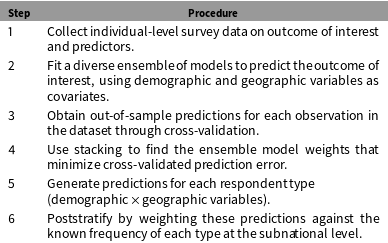
Once the ensemble weights are estimated, Equation (1) produces the first-stage predictions. The local-area estimates can then be generated through poststratification as in classical MRP. Table 1 summarizes the SRP procedure.
Table 1. The SRP Procedure.
3 Monte Carlo Simulation
How well does SRP perform relative to classical MRP? And under what conditions does it perform best? To address these questions, I conduct a Monte Carlo analysis, simulating a data generating process where the outcome variable ( $\mathbf{y}$) is a function of two individual-level covariates ( $\mathbf{z}_{\mathbf{1}}$, $\mathbf{z}_{\mathbf{2}}$), one unit-level covariate ( $\boldsymbol{\unicode[STIX]{x1D706}}$), and a stylized geographic location. The DGP is linear-additive except in two geographic regions, where the $Z$ variables have a multiplicative effect.Footnote 3 This produces a pattern that one might expect to observe in real data, where the relationship between demography, geography, and public opinion is not well captured by a linear and additively separable model (e.g. income is strongly associated with voting Republican in Mississippi, but weakly associated in Connecticut (Gelman et al. Reference Gelman, Shor, Bafumi and Park2007)).
More formally, the data are generated through the following process. First, I create  $NM$ individuals, where $M$ is the number of subnational units, and $N$ is the number of observations per unit. Each individual has four latent (unobserved) characteristics, $z_{1}$ through $z_{4}$, drawn from a multivariate normal distribution with mean zero and variance–covariance matrix equal to
 $$\begin{eqnarray}\left[\begin{array}{@{}cccc@{}}1 & \unicode[STIX]{x1D70C} & \unicode[STIX]{x1D70C} & \unicode[STIX]{x1D70C}\\ \unicode[STIX]{x1D70C} & 1 & \unicode[STIX]{x1D70C} & \unicode[STIX]{x1D70C}\\ \unicode[STIX]{x1D70C} & \unicode[STIX]{x1D70C} & 1 & \unicode[STIX]{x1D70C}\\ \unicode[STIX]{x1D70C} & \unicode[STIX]{x1D70C} & \unicode[STIX]{x1D70C} & 1\end{array}\right].\end{eqnarray}$$
 The variable  $\mathbf{z}_{\mathbf{4}}$ is used to assign each observation to a subnational unit, which ensures that there is cross-unit variation on the latent characteristics. Each subnational unit, in turn, is assigned a random latitude and longitude, drawn from a bivariate uniform distribution between $(0,0)$ and $(1,1)$. Once I assign each observation a $\mathbf{z}$ vector and subnational unit, I generate the outcome variable, $y$, using the following equation:
 $$\begin{eqnarray}y_{i}=z_{1i}+z_{2i}+z_{3i}+\unicode[STIX]{x1D703}(D_{i}^{0}z_{1i}z_{2i}-D_{i}^{1}z_{1i}z_{3i})+\unicode[STIX]{x1D700}_{i}.\end{eqnarray}$$ $D^{0}$ is a function that is decreasing in distance from (0,0), and $D^{1}$ is decreasing in distance to (1,1), so that multiplicative effects are strongest near those points. $\unicode[STIX]{x1D700}_{i}$ is an iid normal error term with mean zero and variance $\unicode[STIX]{x1D70E}^{2}$. The parameter $\unicode[STIX]{x1D703}$ governs the strength of the three-way interaction effect. When $\unicode[STIX]{x1D703}=0$, the DGP is simply a linear-additive combination of the demographic variables, but as $\unicode[STIX]{x1D703}$ increases, the conditional effect of geography becomes stronger. Finally, I create discretized versions of the demographic variables $\mathbf{z}_{\mathbf{1}}$ through $\mathbf{z}_{\mathbf{3}}$, called $\mathbf{x}_{\mathbf{1}}$ through $\mathbf{x}_{\mathbf{3}}$. Although the outcome variable $y$ is a function of the latent variables, $Z$, the researcher can only observe the discrete variables $X$. In addition, the researcher cannot observe $\mathbf{x}_{\mathbf{3}}$ at the individual level, but instead observes its unit-level means ( $\unicode[STIX]{x1D706}_{m}$), which are included as a predictor in the first-stage model.
I repeatedly simulate this data generating process, varying the parameters  $\unicode[STIX]{x1D70C}$ and $\unicode[STIX]{x1D703}$. (See the Supplementary Materials for a more detailed technical description of the Monte Carlo and the combinations of parameter values used.) For each simulated population, I then draw a random sample of size $n$ and generate three sets of subnational estimates: disaggregation, classical MRP, and SRP. The first-stage equation for the MRP estimation is a multilevel regression model of the following form, where $x_{1}$ and $x_{2}$ are the individual-level covariates and $\unicode[STIX]{x1D6FC}_{m}^{\text{unit}}$ is a unit-specific intercept, itself a function of the unit-level covariate, $\unicode[STIX]{x1D706}_{m}$:
 $$\begin{eqnarray}\displaystyle & \displaystyle y_{i}=\unicode[STIX]{x1D6FD}^{0}+\unicode[STIX]{x1D6FC}_{j}[i]^{x_{1}}+\unicode[STIX]{x1D6FC}_{k}[i]^{x_{2}}+\unicode[STIX]{x1D6FC}_{m}^{\text{unit}}+\unicode[STIX]{x1D700}_{i}; & \displaystyle \nonumber\\ \displaystyle & \displaystyle \unicode[STIX]{x1D6FC}_{j}^{x_{1}}\sim N(0,\unicode[STIX]{x1D70E}_{j}^{2}); & \displaystyle \nonumber\\ \displaystyle & \displaystyle \unicode[STIX]{x1D6FC}_{k}^{x_{2}}\sim N(0,\unicode[STIX]{x1D70E}_{k}^{2}); & \displaystyle \nonumber\\ \displaystyle & \displaystyle \unicode[STIX]{x1D6FC}_{m}^{\text{unit}}\sim N(\unicode[STIX]{x1D6FD}^{\unicode[STIX]{x1D706}}\cdot \unicode[STIX]{x1D706}_{m},\unicode[STIX]{x1D70E}_{\text{unit}}^{2}). & \displaystyle \nonumber\end{eqnarray}$$
 For the first stage of the SRP, I fit a LASSO using the same predictors as the multilevel model and I train KNN, random forest, and GBM using  $\mathbf{x}_{\mathbf{1}}$, $\mathbf{x}_{\mathbf{2}}$, $\boldsymbol{\unicode[STIX]{x1D706}}_{\mathbf{m}}$, latitude, and longitude as predictors. I use fivefold cross-validation for parameter tuning, and then estimate ensemble model weights through stacking.
Figure 1 illustrates the results of a representative run from the Monte Carlo simulation. Under certain conditions, SRP dramatically outperforms both disaggregation and classical MRP. When  $\unicode[STIX]{x1D703}$ is large—and therefore the multilevel regression model is misspecified—the ensemble model average is better able to predict individual-level opinion than multilevel regression alone, which in turn produces better poststratified estimates.
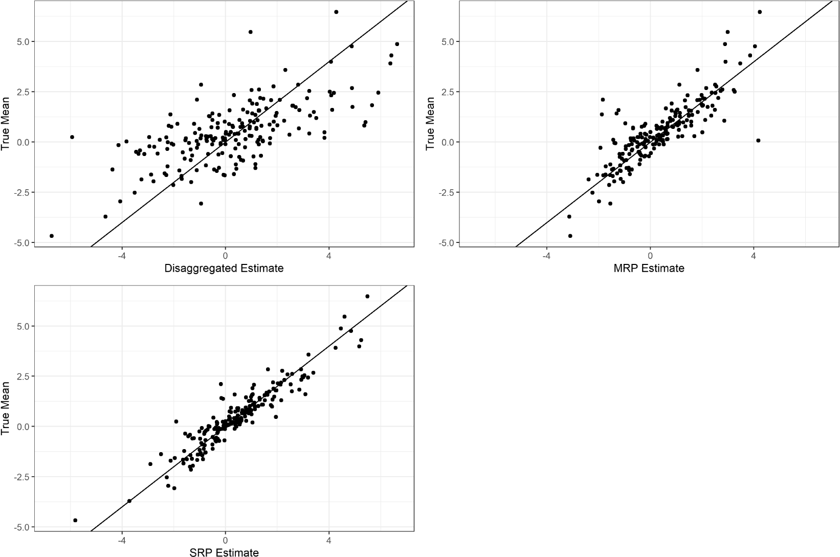
Figure 1. A representative simulation from the Monte Carlo analysis. Disaggregation, MRP, and SRP estimates are plotted against true subnational unit means. Parameter values:  $\unicode[STIX]{x1D703}=5$, $\unicode[STIX]{x1D70C}=0.4$, $N=15\,000$, $M=200$, $n=5000$, $\unicode[STIX]{x1D70E}^{2}=5$.
Note that the component machine learning algorithms do not always perform strictly better than multilevel regression. When  $\unicode[STIX]{x1D703}$ is small—and thus the true DGP is linear-additive—complex models provide no prediction advantage over ordinary least squares. Indeed, the flexibility of methods like KNN become a detriment when the sample size of the survey is small, as KNN performs poorly when the number of predictors is large relative to the size of the training set (Beyer et al. Reference Beyer, Goldstein, Ramakrishnan, Shaft, Beeri and Buneman1999).Footnote 4
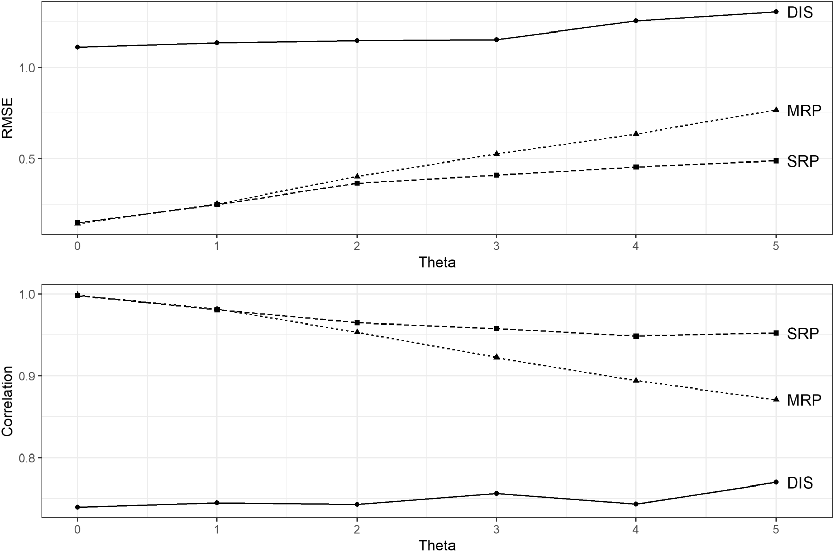
Figure 2. Relative performance of disaggregation, MRP, and SRP estimates, varying  $\unicode[STIX]{x1D703}$. Parameters Used: $\unicode[STIX]{x1D70C}=0.4$, $n=5000$, $M=200$, $N=15\,000$, $\unicode[STIX]{x1D70E}^{2}=5$. Points denote 10-run averages.
Nevertheless, the benefits of SRP can be dramatic under some conditions. In cases where  $\unicode[STIX]{x1D703}$ and $\unicode[STIX]{x1D70C}$ are large, MRP performs only modestly better than disaggregation, while SRP produces estimates that are well-correlated with the true unit means. Figure 2 illustrates these relative performance gains for varying levels of $\unicode[STIX]{x1D703}$. Even when SRP underperforms MRP, it never performs poorly: the worst correlation produced across all simulations was a 0.77 for SRP, compared to 0.78 for MRP and 0.25 for disaggregation.
4 Empirical Application
To demonstrate that SRP produces superior estimates in a wide variety of empirical applications, I replicate the results from Buttice and Highton (Reference Buttice and Highton2013), comparing the performance of SRP and classical MRP. In that study, the authors use MRP to estimate state-level public opinion on 89 issues, drawn from two large-sample surveys of American public opinion, the National Annenberg Election Studies (NAES) and the Cooperative Congressional Election Studies (CCES). Because these surveys collect such a large sample within each state, the authors treat the state-level disaggregated means as the “true” values, and then test how well MRP performs at estimating these values after drawing smaller, random samples from the survey ( $n=1500$ or $n=10\,000$). For each issue area, they model public opinion using a multilevel regression model with sex, age, race, and education as individual-level covariates, state-level covariates on presidential vote share and religious conservatism, and state- and region-specific intercepts.
I replicate this procedure for each of the 89 issue areas using both classical MRP and SRP, varying the size of the random sample drawn ( $n=1500$, 3000, 5000, and 10 000) and repeating the process five times for each combination. The MRP first-stage model is the same as in the original paper. The SRP ensemble includes a LASSO, KNN, random forest, and GBM model, using the same covariates included in Buttice and Highton (Reference Buttice and Highton2013). For the KNN, random forest, and GBM, I substitute the latitude and longitude of each state’s centroid for state- and region-level indicator variables. The stacking procedure typically selects weights that are mixtures of all five models. It is very rare in this empirical application that one model dominated the ensemble; fewer than 8% of ensembles yielded weights where $w_{k}>0.8$ for any model $k$.
$k$.
Figure 3 plots SRP’s performance compared to classical MRP, varying the size of the random sample drawn. Across all simulations, SRP improves correlation in 79% of cases, and reduces mean average error (MAE) in 78% of cases. This performance improvement is the most consistent when working with larger sample sizes (rows 3 and 4). When  $n=10\,000$, SRP outperforms MRP in 88% of cases.

Figure 3. Plots in the left column compare SRP and MRP correlations, varying sample size. Plots in the right column compare Mean Absolute Error.
For issue areas where MRP already performs well, the gains from adopting SRP are modest. This is to be expected; when MRP produces a correlation of 0.9, there can be little improvement from fitting a more sophisticated first-stage ensemble. But in cases where MRP performs poorly, the gains from adopting SRP can be quite substantial. Examining Figure 3, one can observe numerous cases where SRP produces large improvements in correlation or MAE, and very few cases where it performs substantially worse. This is particularly true in Rows 3 and 4, where the estimates are constructed from larger samples.
To consider these performance gains in perspective, Figure 4 reports mean correlation and MAE across simulations, varying sample size. Adopting SRP yields a modest but statistically significant improvement across the board. In some places, this performance gain is comparable to a large increase in sample size. For example, when  $n=5000$, adopting SRP over MRP increases the correlation from 0.68 to 0.72. This performance gain is comparable to doubling the sample size to $n=10\,000$, a feat that is much more difficult in practice. (Doing both is, of course, best of all.)
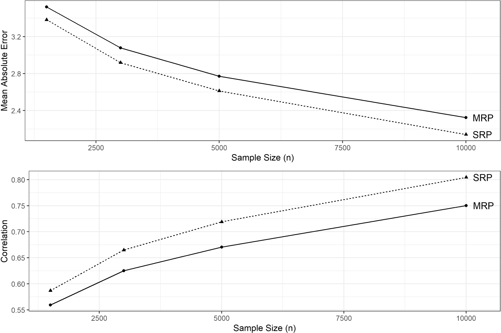
Figure 4. Mean performance of SRP and MRP across all simulations, varying sample size.
The core finding from Buttice and Highton (Reference Buttice and Highton2013) is that MRP’s performance can be highly variable when using national-level surveys with a typical sample size of  $n=1500$. This remains true for SRP, albeit to a lesser extent. As the empirical application demonstrates, SRP performs best with large sample size. This is to be expected, given that more complex models require more data to fit. But it suggests that SRP alone is insufficient to expect good estimates from small, unrepresentative public opinion surveys. Rather, researchers should be most confident in estimates produced from large-sample surveys and cross-validated first-stage models.
5 Conclusion
In both Monte Carlo and empirical applications, SRP produces modest but consistent performance gains over classical MRP. These gains are largest in cases where the data generating process is complex, with nonlinear interactions between demographic and geographic variables that are unlikely to be specified in advance by the researcher’s model. In the empirical analysis, SRP performs markedly better on issue areas where MRP performed poorly in Buttice and Highton (Reference Buttice and Highton2013).
Despite this improvement in prediction performance, there are two reasons why a researcher might choose to forego SRP and employ classical MRP instead. The first involves “synthetic poststratification”, a method proposed by Leemann and Wasserfallen (Reference Leemann and Wasserfallen2017). This refinement of MRP proceeds as if the joint distribution of individual-level covariates is simply the product of their marginal distributions, allowing the researcher to include additional individual-level predictor variables in the first-stage model. In the Supplementary Materials (Appendix A), I prove that this procedure and classical MRP produce identical estimates, but only if the first-stage model is linear-additive. This suggests that, for applications where the researcher must conduct the poststratification stage synthetically —e.g. in countries that do not publish detailed census microdata— it is prudent to use a linear-additive model for the first-stage predictions rather than the ensemble methods proposed here.
The second cost of SRP is its added computational complexity; it takes significantly longer to estimate an ensemble of models than it does to estimate a single regression model. This is particularly true when gradient boosting is included in the ensemble, as it requires the most computationally intensive parameter tuning of all the methods I survey here (see the Supplementary Materials for details). To produce the results in this paper, I conducted several thousand simulations, which required a significant amount of computation time. But for applied researchers who need only to generate a single set of estimates, the added computation time is negligible. The maximum time spent on a single run was 15 minutes, the majority of which was spent tuning the GBM parameters. The average run time was closer to 3 minutes.
Given these results, I strongly recommend that researchers consider using SRP in place of MRP, particularly when working with large ( $n>5000$) public opinion datasets like CCES or NAES. To facilitate this, readers are welcome to adapt my replication code for their use, and I have developed an R package (SRP) currently available on my website. Ultimately, I hope that SRP will prove to be a useful addition to the empirical social scientist’s toolkit, spurring further research into subnational politics.
Acknowledgements
The author thanks Rob Franzese, Scott Page, Liz Gerber, Paul Kellstedt, the anonymous reviewers, and workshop participants at the University of Michigan and the Midwest Political Science Association for their helpful comments and suggestions on earlier drafts.
Supplementary Material
For supplementary material accompanying this paper, please visit https://doi.org/10.1017/pan.2019.43.


