


If you want to pick cherries, go where
the cherries is.
Matthew Reese, Executive Director of
Citizens for Kennedy
1 Introduction
Scholars and pundits alike have long been captivated by “swing voters”: a niche group of voters who are undecided or otherwise could be persuaded to switch their support between candidates or parties. Pollsters routinely tag these voters using a colorful taxonomy: soccer moms, Reagan Democrats, and so forth. Likewise, research into the political behavior of swing voters has spanned the entire course of modern political science, beginning with the pioneering voter panel studies of the Columbia school (Lazarsfeld, Berelson, and Gaudet Reference Lazarsfeld, Berelson and Gaudet1944). In short, both campaigns and political scientists have a keen interest in identifying the “cherries” of the electorate.
Although they have long captured the political imagination, swing voters have remained an enigmatic player in American politics. At times, swing voters are idealized as model citizens—a thoughtful, fair, open-minded, and dispassionate force for reasoned discourse and moderation in American democracy. However, one can also point to a legion of findings documenting depressed levels of political information and interest among swing voters. Recent work also emphasizes the role of partisan polarization in clarifying the major party brands and reducing the number of swing voters in contemporary American elections (e.g., Gelman et al. Reference Gelman, Goel, Rivers and Rothschild2016; Smidt Reference Smidt2017).Footnote 1
Before we can learn about swing voters, we must first be able to identify them. More than 70 years of theory has established cross-pressuring as a key motivator of swing voting (Berelson, Lazarsfeld, and McPhee Reference Berelson, Lazarsfeld and McPhee1954; Campbell et al. Reference Campbell, Converse, Miller and Stokes1960; Key Jr. Reference Key1966). These cross-pressures are complex entities that involve friction between partisan, demographic, social, and attitudinal elements. Recent work demonstrates that cross-pressures remain pervasive among voters, even in the face of partisan polarization (e.g., Brader, Tucker, and Therriault Reference Brader, Tucker and Therriault2014; Hillygus and Shields Reference Hillygus and Shields2008).
In voting behavior models, these cross-pressures are manifest as (often high-order) interaction terms that are difficult to detect using standard regression-based approaches. Instead, we argue that an ensemble machine learning approach—one that combines insights from a variety of supervised methods—provides a more flexible and theoretically superior means of modeling the complex mechanisms driving swing voter behavior.
We test the effectiveness of a learning ensemble in predicting swing voter propensity using longitudinal survey data between 2011 and 2019. Our analysis reveals two main findings: first, the ensemble model identifies an individual-level disposition toward swing voting that is predictive (1) for out-of-sample respondents, (2) across related behaviors such as split-ticket voting, and (3) of swing voting in later elections. We attribute the learning ensemble’s success to its ability to identify consequential cross-pressures among voters. In short, swing voters exist, and this propensity can be measured with an appropriate modeling strategy.
Second, we find that policy-related considerations (specifically, measures of ideological identification, issue preferences, and issue salience) are essential for accurately predicting swing voters. The results indicate that policy attitudes are a key component of swing voting behavior, even if their influence often cannot be characterized in simple linear terms. Swing voting arises not only among voters who lack partisan attachments or political sophistication, but also those who experience conflict between the parties on salient policy issues (see also Green Reference Green2020).
2 Swing Voters and Cross-Pressures
The study of swing voters has its origins in the seminal works of the Columbia school of voting behavior (Berelson et al. Reference Berelson, Lazarsfeld and McPhee1954; Lazarsfeld et al. Reference Lazarsfeld, Berelson and Gaudet1944).Footnote 2 One pioneering aspect of these studies concerns their discussion of “cross-pressures”: competing factors or considerations that introduce ambivalence into voters’ decisionmaking processes. Voters facing cross-pressures exhibit greater volatility their vote intentions: they are more likely to change their minds and remain undecided over the course of the campaign. Consequently, cross-pressured voters’ final decisions often turn on short-term factors or personal salience—which candidate or party aligns with the set of considerations the voter considers most important (Petrocik, Benoit, and Hansen Reference Petrocik, Benoit and Hansen2003; RePass Reference RePass1971; Zaller Reference Zaller, Saris and Sniderman2004).
More recent work also indicates that demographically (Brader et al. Reference Brader, Tucker and Therriault2014) and ideologically (Treier and Hillygus Reference Treier and Hillygus2009) cross-pressured voters hold more ambivalent political preferences. Such cross-pressures are also widespread in the American electorate: about two-thirds of partisans disagree with their party on at least one issue they consider important, with 40 $\%$
of partisans disagreeing on two or more personally salient issues (Hillygus and Shields Reference Hillygus and Shields2008; see also Lupton, Myers, and Thornton Reference Lupton, Myers and Thornton2015). A sizable proportion of American voters also hold incongruent symbolic and operational ideological preferences (Ellis and Stimson Reference Ellis and Stimson2012). The diversity of issue publics in the American electorate provides yet another source of tension in the multidimensional lattice of voters’ policy attitudes (Klar Reference Klar2014; Krosnick Reference Krosnick1990).
$\%$
of partisans disagreeing on two or more personally salient issues (Hillygus and Shields Reference Hillygus and Shields2008; see also Lupton, Myers, and Thornton Reference Lupton, Myers and Thornton2015). A sizable proportion of American voters also hold incongruent symbolic and operational ideological preferences (Ellis and Stimson Reference Ellis and Stimson2012). The diversity of issue publics in the American electorate provides yet another source of tension in the multidimensional lattice of voters’ policy attitudes (Klar Reference Klar2014; Krosnick Reference Krosnick1990).
A number of factors—most importantly, party identification and political sophistication—serve to inoculate voters from the effects of cross-pressures and promote stability in voting behavior. Indeed, much of the literature on swing or “floating” voters focuses on these voters’ lack of partisan attachments and political knowledge to explain their susceptibility to cross-pressuring (Converse Reference Converse1962; Mayer Reference Mayer2007). However, these factors also interact with each other and the political environment in complex ways to influence swing voter behavior. For instance, intensely polarized campaigns can harden partisan identities, but can also serve to inform or remind cross-pressured partisans of inconsistencies in their political choices (Box-Steffensmeier et al. Reference Box-Steffensmeier, Dillard, Kimball and Massengill2015). In fact, campaign efforts to prime specific considerations are most effective among voters with moderate and especially high levels of political awareness in the United States (Claassen Reference Claassen2011) and comparative contexts (Dassonneville and Dejaeghere Reference Dassonneville and Dejaeghere2014; Weghorst and Lindberg Reference Weghorst and Lindberg2013). Accordingly, although cross-pressured partisans tend to hold lower levels of political information (Claassen and Highton Reference Claassen and Highton2009), cross-pressures are likely most consequential for knowledgeable partisans—especially when the issue is salient(Carsey and Layman Reference Carsey and Layman2006).
Determining the extent to which policy considerations underlie swing voter propensity has meaningful normative implications. If swing voters are politically alienated and lack meaningful policy views, then they may simply be “electoral drifters or rolling stones, who cast their vote almost at random” (Katz, Rattinger, and Pedersen Reference Katz, Rattinger and Pedersen1997, 87). On the other hand, policy preferences may systematically influence swing voter propensity, but do so in nuanced (interactive) ways whose detection require a more sophisticated modeling approach. If so, swing voters may be more pervasive and receptive to policy-based appeals than commonly believed.
3 A Learning Ensemble Strategy to Identify Swing Voters
Existing work demonstrates that swing voters are a heterogeneous group whose choices are motivated by complex interactions between a set of factors—namely, demographic and attitudinal cross-pressures, issue salience, political sophistication, strength of partisan ties, cross-cutting social affiliations and identities, and ideological moderation. The forces driving swing voter propensity are likely to take the form of complex nonlinear and conditional patterns—patterns that could be easily overlooked by researchers employing traditional regression models. In such cases, relaxing functional form assumptions can enhance inference and reveal new possibilities for investigation (Wager and Athey Reference Wager and Athey2018).
This consideration motivates our use of an alternative, flexible supervised machine learning-based estimation strategy to detect the pairings of attributes and attitudes that theory suggests underlie swing voter behavior. These methods allow us to test the possibility that nonlinear and interactive relationships predict swing voting. Social scientists are more frequently adopting machine learning to discover patterns and identify meaningful relationships in data—especially those involving complex patterns in the data generating process.Footnote 3
Below we detail our use of a learning ensemble—one that combines insights from multiple supervised machine learning methods—to study swing voter behavior. Ensemble methods have revolutionized the fields of predictive modeling and statistical learning over recent decades, advanced through theoretical work (Schapire Reference Schapire1990) alongside the development of specific procedures such as stacking (Wolpert Reference Wolpert1996), bagging (Breiman Reference Breiman1996), boosting (Freund and Schapire Reference Freund and Schapire1997), and super learners (van der Laan, Polley, and Hubbard Reference van der Laan, Polley and Hubbard2007). Ensembling is based on a key insight sometimes referred to as the “wisdom of crowds”: a diverse set of component methods, each with their own assumptions about the underlying data generating process, can capture different aspects of the relationship between predictor and response variables (Ali and Pazzani Reference Ali and Pazzani1996). Aggregating their results into an ensemble smooths over idiosyncratic errors produced by the component methods (or base learners), producing a lower variance estimator. Hence, the goal of ensemble methods is to find the combination of base learners that optimizes generalizable (i.e., out-of-sample) predictive performance.
To accomplish this, we follow the approach developed in Grimmer, Messing, and Westwood (Reference Grimmer, Messing and Westwood2017) to estimate the component weights for a series of supervised machine learning methods trained to predict swing voting. Formally, let i index the observations ( $i=1,\ldots ,n$
) and m index the component methods (
$i=1,\ldots ,n$
) and m index the component methods ( $m=1,\ldots ,M$
). We first randomly divide the N observations into D (
$m=1,\ldots ,M$
). We first randomly divide the N observations into D ( $d=1,\ldots ,D$
) folds, and generate predictions for observations in each fold d by fitting the M methods on observations in the remaining
$d=1,\ldots ,D$
) folds, and generate predictions for observations in each fold d by fitting the M methods on observations in the remaining $D-1$
folds. This produces an
$D-1$
folds. This produces an $N \times M$
matrix of out-of-sample predictions (
$N \times M$
matrix of out-of-sample predictions ( $\hat {Y}_{im}$
) for each observation across the component methods. We then estimate the component weights (
$\hat {Y}_{im}$
) for each observation across the component methods. We then estimate the component weights ( $w_{m}$
) by fitting the constrained regression problem:
$w_{m}$
) by fitting the constrained regression problem:
 $$ \begin{align} Y_{i} = \sum_{m=1}^{M} w_{m} \hat{Y}_{im} + \epsilon_{i}, \end{align} $$
where $Y_{i}$
is the observed response by respondent i and
$Y_{i}$
is the observed response by respondent i and $\epsilon _{i}$
is a stochastic error term, with the constraints that
$\epsilon _{i}$
is a stochastic error term, with the constraints that $\sum _{m=1}^{M}w_{m}=1$
and
$\sum _{m=1}^{M}w_{m}=1$
and $w_{m} \geq 0$
. Finally, we fit each of the component methods to the complete dataset and weight the predictions using the M-length vector of estimated component weights
$w_{m} \geq 0$
. Finally, we fit each of the component methods to the complete dataset and weight the predictions using the M-length vector of estimated component weights $\hat {\textbf {w}}$
. The weighted combination of predictions comprise the ensemble estimates.
$\hat {\textbf {w}}$
. The weighted combination of predictions comprise the ensemble estimates.
In our analysis, we use an ensemble of eight component methods (or base learners) to model the relationship between swing voting and a series of predictor variables. These include a standard additive probit regression model, k-nearest neighbors, group-lasso interaction network, support vector machine (SVM), neural networks, random forests, gradient-boosted decision trees, and extremely randomized trees.Footnote 4 We describe the component methods and weights in greater detail in Appendix B in the Supplementary Material, but it is worth emphasizing that these procedures range in complexity and each bring strengths to the ensemble. For instance, SVMs and neural networks excel in fitting nonlinear mappings between X and Y by estimating various transformations of the input data whereas the group-lasso interaction network and tree-based methods are robust to irrelevant predictors (Hastie, Tibshirani, and Friedman Reference Hastie, Tibshirani and Friedman2009, 350–352; Kuhn and Johnson Reference Kuhn and Johnson2013, 488–490, 550).
Given our theoretical expectations about the role of cross-pressures on swing voting, it is also important to emphasize that the tree-based methods provide a natural way to model interactive relationships, since the effect of any given variable is considered conditionally based on previous splits in the tree. This helps to explain why decision trees are so effective in uncovering interactive effects and modeling the behavior of heterogeneous groups like swing voters (Lampa et al. Reference Lampa, Lind, Lind and Bornefalk-Hermansson2014; Montgomery and Olivella Reference Montgomery and Olivella2018). The ensemble harnesses the strengths of each base learner in a single prediction function, one that can be validated and probed as described below.
4 Predicting Swing Voters in Presidential Elections
We train our component methods and construct our learning ensemble using data from the 2012 Cooperative Campaign Analysis Project (CCAP; Jackman et al. Reference Jackman, Sides, Tesler and Vavreck2012).Footnote 5 The 2012 CCAP interviewed a group of 43,998 respondents with a rolling cross-section design at three points during the 2012 campaign: a baseline survey in December 2011, a weekly interview between January and November 2012, and a post-election survey. Beyond its large sample size, the 2012 CCAP is ideal for our purposes, because it allows us to fit the learning ensemble to only the variables collected during the baseline survey, then evaluate the model’s performance in predicting subsequent behavior during and immediately following the 2012 election. Four-thousand seven-hundred and fifteen of these respondents are also panelists in a long-term survey conducted by the Democracy Fund (the VOTER Study Group; Democracy Fund Voter Study Group 2020), allowing us to validate the model using vote choice/intention measures from the 2016 and 2020 presidential elections.
The 2012 CCAP asked a wide set of political questions concerning past turnout and vote choice; candidate evaluations and ideological and party identification; issue preferences; political knowledge and interest; racial resentment; economic evaluations; and personal issue salience. We also construct a measure of ideological inconsistency based on Federico and Hunt’s (Reference Federico and Hunt2013) operationalization. In all, we include 45 predictor variables (detailed in Appendix A in the Supplementary Material) that theory suggests are related to swing voting and were included in the baseline wave of the 2012 CCAP.
To construct our measure of swing voting, we look for manifest behaviors that serve as indicators of a voter’s latent propensity to switch between electoral choices. As Mayer (Reference Mayer and Mayer2008, 2) defines the concept: “In simple terms, a swing voter is, as the name implies, a voter who could go either way: a voter who is not so solidly committed to one candidate or the other as to make all efforts at persuasion futile.” Following Weghorst and Lindberg (Reference Weghorst and Lindberg2013), we include two commonly used markers of swing voting: party switching and indecision (i.e., undecided voters).Footnote 6 In line with Mayer’s (Reference Mayer and Mayer2008) definition, both behaviors indicate that a voter’s preferences meet a meaningful threshold of volatility. By providing the learning ensemble multiple instances of the concept under investigation, it has greater leverage to uncover the complex patterns underlying swing voter propensity.Footnote 7
Specifically, our response variable codes swing voters as those respondents who fully or temporarily defected from their 2008 presidential vote choice in the following ways:
-
1. Full defectors: respondents who voted for Obama (McCain) in the 2008 presidential election, but switched to the other party and voted for Romney (Obama) in 2012. This corresponds to the standard operationalization of floating voters.
-
2. Temporary defectors: respondents who voted for the same party in the 2008 and 2012 presidential elections, but stated that they were undecided or intended to switch to the other party’s candidate at some point during the 2012 campaign.
This operationalization produces 2,294 respondents whom we classify as swing voters, compared to the 14,881 respondents who expressed party-consistent preferences across the 2008 and 2012 presidential elections coded as non-swing voters. Of these respondents, 12,914 have complete, non-missing profiles across the predictor and response variables. We select a random 65 $\%$
(8,395) of these respondents to create the training set, leaving 4,519 respondents to comprise the validation set. The training set is used to estimate the learning ensemble, whereas the validation set is used to assess the model’s out-of-sample performance.
$\%$
(8,395) of these respondents to create the training set, leaving 4,519 respondents to comprise the validation set. The training set is used to estimate the learning ensemble, whereas the validation set is used to assess the model’s out-of-sample performance.
We estimate and tune the component models using 10-fold cross-validation (repeated five times) using area under the receiver operating characteristic curve (AUC-ROC) as our performance metric. The learning ensemble selects four methods (with component weights in parentheses): extremely randomized trees ( $w=0.32$
), gradient-boosted trees (
$w=0.32$
), gradient-boosted trees ( $w=0.27$
), group-lasso interaction network (
$w=0.27$
), group-lasso interaction network ( $w=0.23$
), and the SVM classifier (
$w=0.23$
), and the SVM classifier ( $w=0.17$
). Hence, the ensemble scores are weighted sums of the predictions from these methods. In the next section, we assess the generalizability of the learning ensemble, specifically how well it predicts swing voting among different respondents and across different electoral contexts. This is of course key to the quality of any substantive inferences that can be drawn from the model concerning general patterns of swing voting in the electorate.
$w=0.17$
). Hence, the ensemble scores are weighted sums of the predictions from these methods. In the next section, we assess the generalizability of the learning ensemble, specifically how well it predicts swing voting among different respondents and across different electoral contexts. This is of course key to the quality of any substantive inferences that can be drawn from the model concerning general patterns of swing voting in the electorate.
4.1 Validating the Swing Voter Scores
In this section, we exclusively use the 4,519 observations in the validation set to assess the out-of-sample predictive accuracy of the learning ensemble. We also compare the ensemble’s performance to a baseline model, using a generalized additive model (GAM) using splines to generate a second set of swing voter predictions.Footnote 8 We are interested in how well each model predicts swing voting as defined by our measure and as evidenced in related behaviors such as split-ticket voting.
As detailed in Table 1, we use a variety of fit metrics to evaluate classifier performance. Given the large class imbalance (only 13 $\%$
of the respondents in both the training and validation sets are classified as swing voters), we focus on metrics other than simple accuracy that measure different desirable qualities of a prediction model. While AUC-ROC provides an indicator of a model’s discriminatory power (how well it separates predictions for observations in each class), Brier skill scores (BSSs) are used to assess calibration: the consistency between the predicted and observed class proportions. Both discrimination and calibration should be considered when evaluating the quality of predictive models (e.g., Bansak Reference Bansak2019). The final two metrics—the Matthews correlation coefficient (MCC) and cross-entropy (CE) loss—both describe the strength of association between the model predictions (the swing voter propensity scores) and the response variable.
$\%$
of the respondents in both the training and validation sets are classified as swing voters), we focus on metrics other than simple accuracy that measure different desirable qualities of a prediction model. While AUC-ROC provides an indicator of a model’s discriminatory power (how well it separates predictions for observations in each class), Brier skill scores (BSSs) are used to assess calibration: the consistency between the predicted and observed class proportions. Both discrimination and calibration should be considered when evaluating the quality of predictive models (e.g., Bansak Reference Bansak2019). The final two metrics—the Matthews correlation coefficient (MCC) and cross-entropy (CE) loss—both describe the strength of association between the model predictions (the swing voter propensity scores) and the response variable.
Table 1 Description and interpretation of model predictive performance metrics.
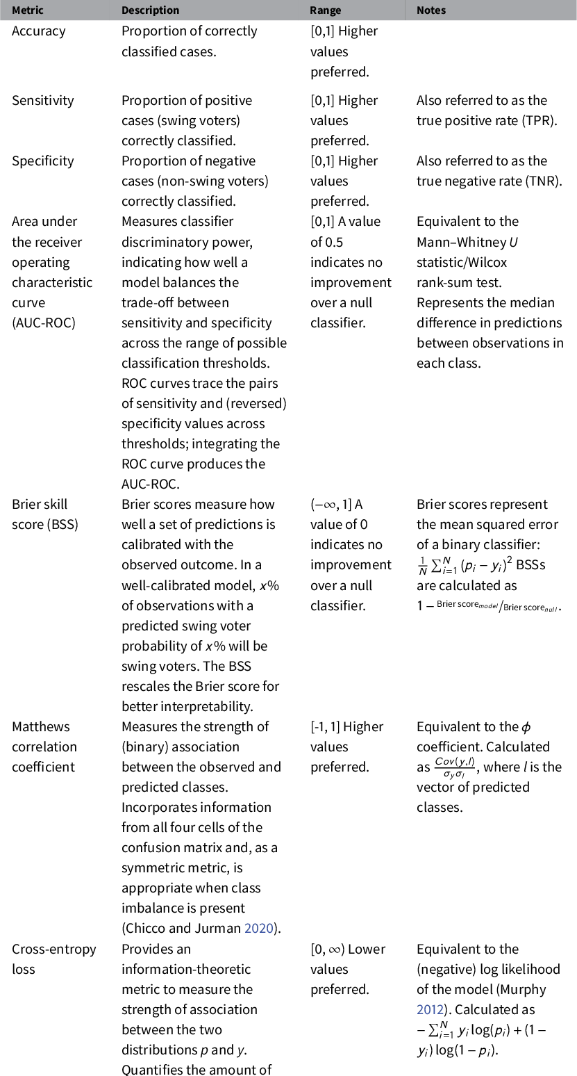
Notes: y = response variable, p = predicted probabilities (positive class), l = predicted classes.
The performance metrics for our main measure of swing voting are presented in Table 2. Alongside the learning ensemble and baseline GAM, we also include the individual base learners that comprise the ensemble. Across the four key aggregate metrics (AUC-ROC, BSS, MCC, and CE loss), Table 2 shows that the ensemble outperforms both the GAM and its component methods. The learning ensemble especially outperforms the baseline GAM in terms of its ability to detect the swing voters in the sample (sensitivity rates of 0.57 vs. 0.22). While two of the base learners (ERT and GBM) have greater sensitivity than the ensemble, they also tend to overpredict swing voting and achieve lower specificity rates. The learning ensemble balances both goals, creating a more discriminatory and better calibrated set of swing voter propensity scores.Footnote 9
Table 2 Model performance on the out-of-sample (validation) data.

This smoothing effect is also seen in Figure 1, which isolates the ROC and calibration curve plots for the learning ensemble and GAM. Two calibration plots are shown: the top panel uses the raw predictions from each model, whereas the bottom panel uses Platt scaling to calibrate the predictions with a logistic transformation (Platt Reference Platt, Smola, Bartlett, Schöelkopf and Schuurmans2000).Footnote 10 Focusing first on the ROC curves, we find the largest gap between the learning ensemble and GAM occurs in the high-specificity (low false positive rate) region. The GAM is committing many Type II (false-negative) errors, overly classifying respondents as non-swing voters because it misses patterns that are predictive of swing voting.
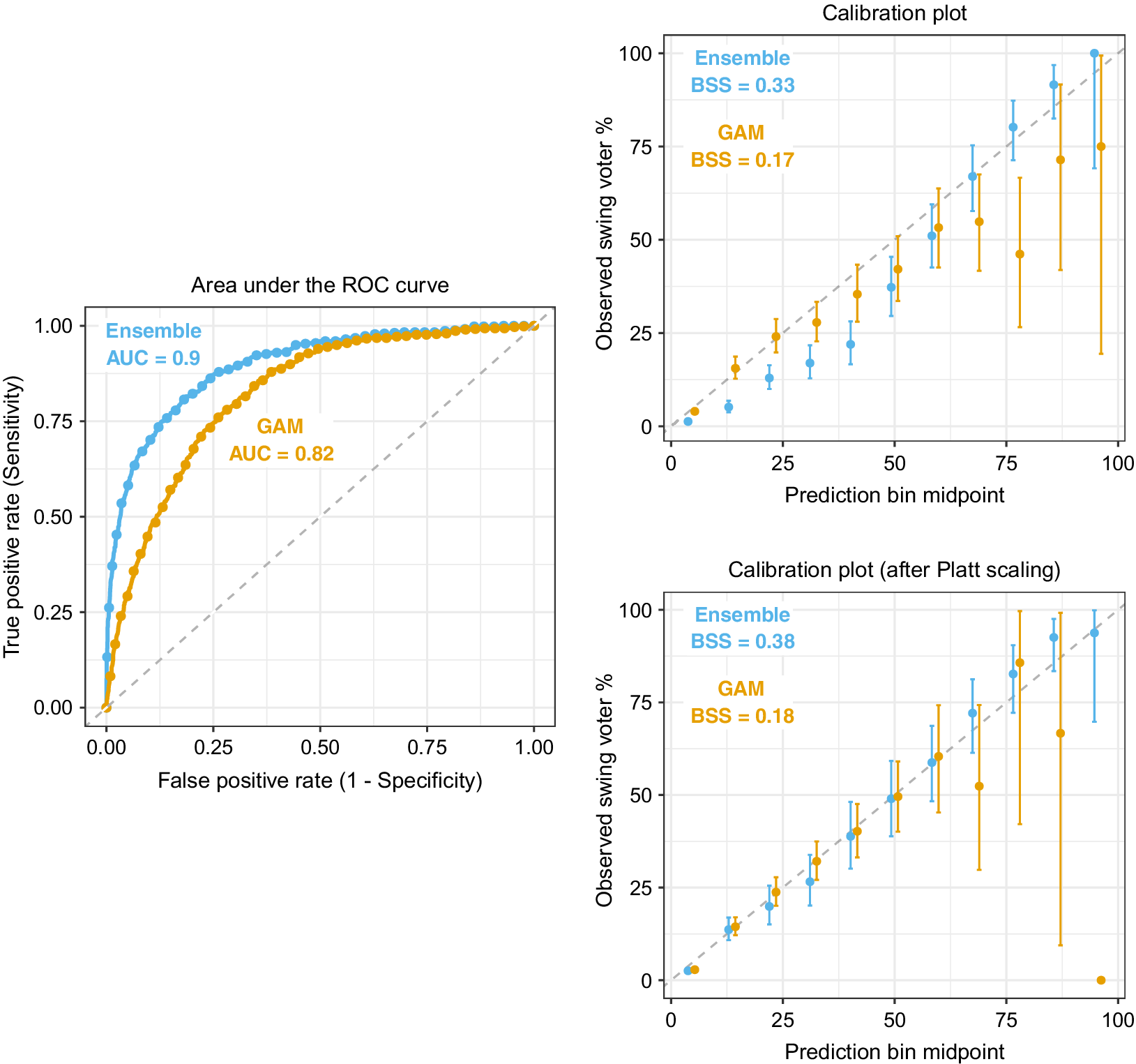
Figure 1 Comparison of the learning ensemble with the baseline generalized additive model (GAM) on the out-of-sample (validation) data. Notes: AUC, area under the ROC curve; BSS, Brier skill score. The bars show 95 $\%$
confidence intervals for the estimated proportions.
$\%$
confidence intervals for the estimated proportions.
The calibration plots in Figure 1b in the respondents based on their swing voter propensity scores and show the percentage of observed swing voters within each bin. The bin midpoints are plotted on the x-axis and the observed swing voter proportions on the y-axis. A perfectly calibrated model will have a curve that overlays the $45^{\circ} $
reference line (e.g., the bin prediction midpoints will exactly match the observed proportions). The top-right panel of Figure 1 shows that the GAM predictions are well calibrated for respondents with low propensity scores, but are noisy and poorly calibrated at higher predicted values. Conversely, the learning ensemble exhibits a sigmoid calibration curve, falling slightly below (above) the reference line at lower (higher) predicted values.
$45^{\circ} $
reference line (e.g., the bin prediction midpoints will exactly match the observed proportions). The top-right panel of Figure 1 shows that the GAM predictions are well calibrated for respondents with low propensity scores, but are noisy and poorly calibrated at higher predicted values. Conversely, the learning ensemble exhibits a sigmoid calibration curve, falling slightly below (above) the reference line at lower (higher) predicted values.
The BSSs confirm that the learning ensemble provides better calibrated predictions than the GAM (BSS values of 0.33 vs. 0.17), but especially given the ensemble calibration curve’s sigmoid pattern, we can achieve further improvement in model calibration by applying Platt scaling to transform the predictions. The ensemble’s transformed predictions exhibit much greater correspondence between the observed and predicted proportions of swing voters for the learning ensemble (its BSS value jumps from 0.33 to 0.38 following Platt scaling). The improvement in calibration for the GAM model is only marginal (an increase in BSS from 0.17 to 0.18).
We next evaluate the ensemble by assessing its predictive performance on 12 indicators related to swing voter propensity. These include measures of attitudinal ambivalence, split-ticket voting, and swing voting in non-presidential elections (Mulligan Reference Mulligan2011). This is a more rigorous test of the ensemble, since it is performed on variables distinct from the specific swing voter measure in the model. Because the 2012 CCAP is a part of a larger panel study (the VOTER Study Group), we can also evaluate how well the propensity scores predict behavior in later election cycles (e.g., swing voting in the 2016 and 2020 presidential elections).
Figure 2 divides the swing voter scores into deciles and shows the proportion of respondents in each percentile who fit the corresponding criteria. For instance, the top-left panel shows that virtually no respondents in the bottom deciles were split-ticket voters in 2012. If the model predictions tap into an underlying swing voter propensity, we should find a monotonic or near-monotonic relationship in each panel. That is, higher scores should correspond to a greater likelihood of swing voter-type behaviors.
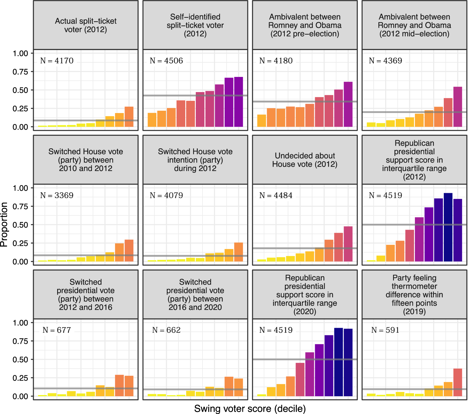
Figure 2 Predictive performance on additional indicators of swing voter propensity using out-of-sample (validation) data. The horizontal bars show the overall proportion of respondents satisfying the corresponding indicator. Ambivalence defined as placing the candidates within one point of each other on a five-point favorability scale. Republican presidential support scores are calculated by estimating ensemble models of 2012 presidential vote choice and 2020 presidential vote intention. Additional details are provided in Appendices D and E in the Supplementary Material.
This is precisely what Figure 2 shows. Moving from left to right in each panel, we find a greater proportion of respondents engaging in split-ticket voting, being undecided or exhibiting volatile preferences in congressional elections, or possessing ambivalent attitudes, and switching between parties across later presidential elections. The predicted scores do not just predict the specific behavior defined by our measure, but other attitudes and choices corresponding to a more volatile electoral profile.
We also use the same predictor variables to estimate a learning ensemble that predicts respondents’ probability of voting for the Republican candidate in the 2012 and 2020 elections. Major political campaigns routinely utilize these methods to generate such support scores for a universe of voters—frequently with the use of decision-tree-based approaches such as chi-square automatic interaction detection (CHAID) and random forests (Nickerson and Rogers Reference Nickerson and Rogers2014). Campaigns often then use those with support scores in the middle range of the scale to identify persuasion targets (Hersh Reference Hersh2015; Issenberg Reference Issenberg2013). These are the voters that campaigns perceive as movable, and consequently they play an outsized role in shaping and implementing campaign strategy (Hersh Reference Hersh2015). We find that our swing voter model converges on many of the same voters that presidential campaigns are likely to view as persuadable (i.e., those with Republican presidential support scores in the interquartile range).
5 Identifying Predictors of Swing Voting
Another promising application of supervised machine learning is an exploratory tool in the model building and evaluation process. Owing to their flexibility, these methods can identify promising predictor variables whose effects have been overlooked either for theoretical reasons or because they are obscured by functional form complexity. That is, a given predictor may share a complex (but nonetheless meaningful) relationship with the response variable that escapes notice when using a series of linear additive terms in a regression model.
Machine learning is already widely used to detect heterogeneous treatment effects in experimental studies (e.g., Green and Kern Reference Green and Kern2012; Montgomery and Olivella Reference Montgomery and Olivella2018). Likewise, these methods can also alert us to meaningful predictors meriting further investigation when we have reasons to believe (as with swing voters) that the data generating process (DGP) is interactive in high-dimensional space. In such cases, Breiman (Reference Breiman2001b) contends that feature importance is best measured using models with high levels of predictive accuracy.Footnote 11 The growing adoption of predictive modeling in the social sciences necessitates tools to probe the results from supervised machine learning algorithms (see generally Bicek and Burzykowski Reference Bicek and Burzykowski2021; Molnar Reference Molnar2019).
In order to gain insight into the factors driving swing voter behavior, below we present two strategies for measuring feature importance in black-box prediction models.Footnote
12
We emphasize that both strategies are model agnostic: they can be used to interrogate any black-box prediction model (or ensemble of models). The unifying principle is that removing a feature $X_{j}$
from a model breaks any meaningful relationship (however, simple or complex) it shares with the response variable y. Comparing model performance before and after removing
$X_{j}$
from a model breaks any meaningful relationship (however, simple or complex) it shares with the response variable y. Comparing model performance before and after removing $X_{j}$
then provides an estimate of that feature’s contribution to the ensemble that can be interpreted in information-theoretic terms. This basic strategy unifies a broad set of specific techniques for black-box model explanation, as discussed in (Covert, Lundberg, and Lee Reference Covert, Lundberg and Lee2021).Footnote
13
$X_{j}$
then provides an estimate of that feature’s contribution to the ensemble that can be interpreted in information-theoretic terms. This basic strategy unifies a broad set of specific techniques for black-box model explanation, as discussed in (Covert, Lundberg, and Lee Reference Covert, Lundberg and Lee2021).Footnote
13
In the first approach, we proceed by estimating the learning ensemble using all features and generating model predictions. We then simulate each feature’s removal by randomly permuting its values and estimating new model predictions. The difference in model fit (using the same four key metrics presented earlier) provides a permutation-based measure of that feature’s contribution to the ensemble (Breiman Reference Breiman2001a).Footnote 14 In the second approach (sometimes referred to as feature ablation or leave-one-covariate-out), we manually remove a feature (or subset of features) before estimating the ensemble. We then compare the predictive performance of each ablated model to the full model. Though computationally intensive, this technique allows us to assess whether the other predictors can compensate for the loss of information in the omitted features.Footnote 15
Figure 3 shows the mean difference in fit metric for the 20 most influential predictor variables.Footnote
16
The four metrics give similar estimates of feature importance (all pairs correlated at $r \ge 0.92$
), and each identifies party identification as the most predictive characteristic of swing voters. Permutation on partisanship accounts for between 18
$r \ge 0.92$
), and each identifies party identification as the most predictive characteristic of swing voters. Permutation on partisanship accounts for between 18 $\%$
(CE loss) and 30
$\%$
(CE loss) and 30 $\%$
(AUC-ROC) of the total drop-off in ensemble performance.
$\%$
(AUC-ROC) of the total drop-off in ensemble performance.

Figure 3 Feature importance estimates from the learning ensemble. Five-hundred random permutations conducted using out-of-sample (validation) data.
After party identification, the learning ensemble derives a considerable portion of its predictive power from both symbolic and operational ideological factors. This includes ideological self-identification alongside specific policy attitudes (with economic and environmental issue preferences foremost among these). The general ideological inconsistency measure is also highly influential, but the model does not overly rely on this variable to parse out the specific policy cross-pressures driving swing voter propensity. Collectively, the policy-related variables supply between 34 $\%$
(AUC-ROC) and 45
$\%$
(AUC-ROC) and 45 $\%$
(CE loss) of the model’s aggregate predictive power. This effect does not appear to be an artifact of projection (or a “follow the leader” effect) in which voters adopt a preferred candidate or party’s issue stances (e.g., Lenz Reference Lenz2012), as the issue and ideological measures come from the pre-election, baseline wave of the 2012 CCAP.
$\%$
(CE loss) of the model’s aggregate predictive power. This effect does not appear to be an artifact of projection (or a “follow the leader” effect) in which voters adopt a preferred candidate or party’s issue stances (e.g., Lenz Reference Lenz2012), as the issue and ideological measures come from the pre-election, baseline wave of the 2012 CCAP.
The learning ensemble reveals several other influential predictors worth noting, including racial resentment and non-policy “nature of the times” assessments such as right/wrong track attitudes and collective (sociotropic) economic evaluations. This echoes Zaller’s (Reference Zaller, Saris and Sniderman2004) finding that floating voters place greater emphasis on performance-based considerations. Political knowledge, though influential, is not a dominant predictor in the model. Instead, the learning ensemble uses a broader range of features to make predictions and reveals that policy-related considerations are indeed meaningful factors underlying swing voter behavior.
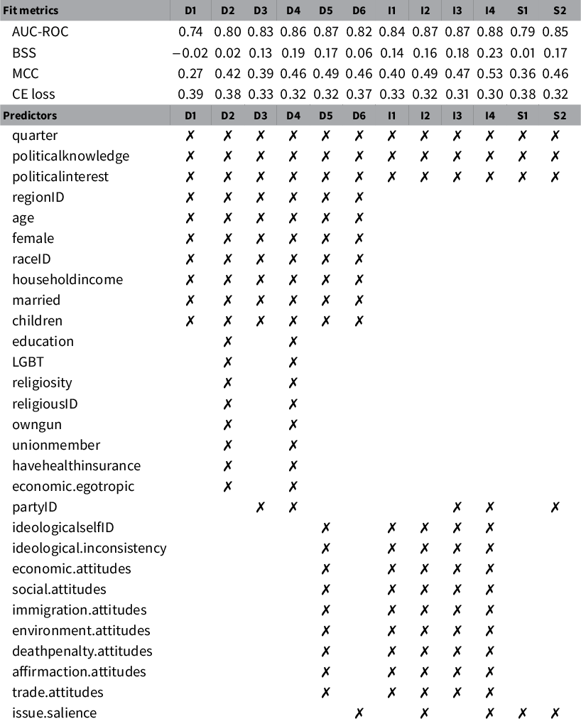
Turning to feature ablation, we predict swing voting by estimating ensemble models (following the same process as above) with 12 combinations of the demographic, issue, and salience items. Table 3 shows the specific predictor variables included in each subset and the corresponding fit statistics. The results support prior claims that information available in public records—variables such as age, voting history, Census block-group statistics, and (in some states) race and party registration—poorly predicts persuadable voters (e.g., Endres Reference Endres2016; Hersh Reference Hersh2015). The subset D1 includes basic demographic variables, including race and political knowledge/interest (predictors that proxy past voting turnout). With this restricted set of variables, the ensemble is both poorly discriminatory (an AUC-ROC of 0.74) and poorly calibrated (a BSS of $-$
0.02). Adding an enhanced set of demographic variables in the subset D2 (which includes predictors such as education and gun ownership that could be proxied with consumer data) increases performance only slightly.
$-$
0.02). Adding an enhanced set of demographic variables in the subset D2 (which includes predictors such as education and gun ownership that could be proxied with consumer data) increases performance only slightly.
Table 3 Learning ensemble performance in predicting swing voters with subsets of predictor variables.

The largest improvements in predictive performance occur once we add party identification and especially policy variables to the ensemble. For instance, subset I4 (which removes demographic variables from the model) produces fit metrics that are in line with those obtained for the full learning ensemble. Consistent with the results from the permutation analysis, a combination of ideological dispositions, policy preferences, and issue salience attitudes are essential to accurately predict swing voters.
6 Discussion
In 1960, a team of political scientists—armed with 130,000 survey responses, a 20-ton IBM 704, and a theory of cross-pressures—began the Simulmatics Project (Pool, Abelson, and Popkin Reference Pool, Abelson and Popkin1964). The project simulated results for the 1960 presidential election by organizing respondents into voter types and estimating how partisan swings resulting from cross-pressures (especially among Protestant Democrats and Catholic Republicans) could affect the outcome. Their predictions were remarkably accurate, demonstrating how cross-pressure theory could be combined with raw computing power to improve models of voting behavior. Pool, Abelson, and Popkin (Reference Pool, Abelson and Popkin1964, pp. 181–182) reflected on the project:
[W]e are moving into an era where the limitation on data bank operations will no longer be computer capacity but only the imagination of the researcher and the extent to which raw data are available to him… The tools that we are now developing can handle models of a complexity adequate to the complexity of the political process itself.
In the same spirit as the Simulatics Project, this paper leverages technological and methodological advancements to explore swing voter behavior in a novel way, using a suite of supervised machine learning methods to search the lattice of cross-pressures permeating the electorate and identifying those most predictive of swing voting. This strategy yields improved estimates of individual swing voter propensity, reiterating the benefits of ensembling and model averaging (e.g., Grimmer et al. Reference Grimmer, Messing and Westwood2017; Montgomery, Hollenbach, and Ward Reference Montgomery, Hollenbach and Ward2012). One possible application of these propensity scores is to improve polling estimates by better identifying swing voters.Footnote 17
However, black-box models need not be limited to pure prediction tasks. Indeed, precisely because these methods are so predictively powerful, they also serve as a valuable exploratory tool—alerting us to untapped information in the data and suggesting new avenues for investigation. As (Grimmer et al. Reference Grimmer, Roberts and Stewart2021, 10) note, “[r]esearchers often discover new directions, questions, and measures within quantitative data… and machine learning can facilitate those discoveries.”
In the application to swing voters, removal-based experimentation on the learning ensemble reveals the importance of policy attitudes in the prediction task. Policy attitudes (specifically, patterns of salient ideological cross-pressures) cannot simply be proxies for other non-policy factors such as partisanship, political sophistication, and demographic characteristics. If this were the case, then the learning ensemble should be able to compensate when policy-related features are removed. Instead, model performance noticeably deteriorates without the pre-election measures of policy attitudes. Using an explicitly predictive modeling strategy, the results demonstrate the difficulty of identifying swing voters without rich individual-level data on voters’ ideological orientations and policy attitudes (cf. Endres Reference Endres2016; Hersh Reference Hersh2015). From a predictive standpoint, the caricature of swing voters as simply politically unaffiliated and uninformed “rolling stones” of the electorate neglects a suite of consequential cross-pressures underlying swing voter behavior.
While the approach presented here is primarily exploratory, future work should continue to unpack the learning ensemble and more formally test-specific high-order cross-pressures involving factors that the ensemble identifies as important.Footnote 18 We think two methods are especially well suited to this task. The first involves the use of causal forests (Wager and Athey Reference Wager and Athey2018) as a semiparametric means of identifying heterogeneous treatment effects for specific features. The second applies the game-theoretic concept of Shapley values—which are concerned with allocating credit to players in coalitional games—to the problem of estimating feature contributions to model predictions (Lundberg et al. Reference Lundberg2020). Both methods are promising options to further enhance ensemble interpretability.Footnote 19
In addition to the specific methodological tools presented here, we also hope that this exercise serves to demonstrate the utility of engaging the study of voting behavior from a predictive modeling standpoint. We can imagine several substantive settings where this approach could reveal other novel insights into existing questions. For instance, in an era of increasingly nationalized political behavior (Hopkins Reference Hopkins2018; though see Kuriwaki Reference Kuriwaki2020), are the same cross-pressures that motivate swing voter propensity at the national level also predictive of volatility in state and local elections?Footnote 20 The ensemble could also further leverage longitudinal data to distinguish between persistent and transitory cross-pressures by evaluating their predictive power across electoral cycles.
Acknowledgments
We would like to thank Bob Ellsworth, Ben Highton, Adrienne Hosek, Bob Lupton, participants in the UC Davis American Politics Reading Group, the editor, and three anonymous reviewers for their helpful feedback.
Data Availability Statement
The replication materials for this paper can be found at https://doi.org/10.7910/DVN/CLQY6O (Hare and Kutsuris Reference Hare and Kutsuris2022).
Supplementary Material
For supplementary material accompanying this paper, please visit https://doi.org/10.1017/pan.2022.24.


 Open access