


1 Introduction
Political scientists often use surveys to estimate and analyze the prevalence of sensitive attitudes and behavior.Footnote 1 To mitigate sensitivity bias in self-reported data (Blair, Coppock, and Moor Reference Blair, Coppock and Moor2020), such as bias arising from social desirability, self-image protection, fear of disclosing truth, and perceived intrusiveness, various survey techniques have been developed including randomized response techniques, list experiments, and endorsement experiments.Footnote 2 The crosswise model is an increasingly popular design among these techniques.Footnote 3 A crosswise question shows respondents two statements: one about a sensitive attitude or behavior of interest (e.g., “I am willing to bribe a police officer”) and one about some piece of private, nonsensitive information whose population prevalence is known (e.g., “My mother was born in January”). The respondents are then asked a question, the answer to which depends jointly on the truth status of both statements and so fully protects respondent privacy (Yu, Tian, and Tang Reference Yu, Tian and Tang2008). The key idea is that even though researchers only observe respondents’ answers to the joint condition, they can estimate the population prevalence of the sensitive attribute using the known probability distribution of the nonsensitive statement.Footnote 4
Despite its promise and several advantages over other indirect questioning techniques (Meisters, Hoffmann, and Musch Reference Meisters, Hoffmann and Musch2020b), recent studies suggest that the crosswise model suffers from two interrelated problems, casting doubt on the validity of the design. First, its relatively complex format leads to a significant share of inattentive survey respondents who give answers that are essentially random (Enzmann Reference Enzmann, Eifler and Faulbaum2017; Heck, Hoffmann, and Moshagen Reference Heck, Hoffmann and Moshagen2018; John et al. Reference John, Loewenstein, Acquisti and Vosgerau2018; Schnapp Reference Schnapp2019; Walzenbach and Hinz Reference Walzenbach and Hinz2019).Footnote 5 Second, this tendency usually results in overestimates of the prevalence of sensitive attributes (Höglinger and Diekmann Reference Höglinger and Diekmann2017; Höglinger and Jann Reference Höglinger and Jann2018; Meisters, Hoffmann, and Musch Reference Meisters, Hoffmann and Musch2020a; Nasirian et al. Reference Nasirian2018). While several potential solutions to this problem have been discussed in the extant literature (Enzmann Reference Enzmann, Eifler and Faulbaum2017; Meisters et al. Reference Meisters, Hoffmann and Musch2020a; Schnapp Reference Schnapp2019), they rely on rather strong assumptions and external information from either attention checks or a different unprotected—but still sensitive—question answered by the same respondents, leading to unsatisfactory solutions.Footnote 6 In this article, we propose an alternative solution that builds on insights about “zero-prevalence items” (Höglinger and Diekmann Reference Höglinger and Diekmann2017) to correct for the bias arising from inattentive respondents.
More generally, we provide the first detailed description and statistical evaluation of methods for measuring and mitigating the bias caused by inattentive respondents in the crosswise model. This includes an evaluation of the performance of our new estimator and a brief assessment of previous methods. Consequently, we not only offer our method as a solution for estimating prevalence rates without bias, but also explain how its assumptions can be easily evaluated and made to hold by design. It also allows us to develop many extensions that enhance its practical usefulness to researchers, including (1) a sensitivity analysis to simulate the amount of bias caused by inattentive respondents even when our correction is not available; (2) a weighting strategy that allows our estimator to be used with general sampling schemes; (3) a framework for multivariate regressions in which a latent sensitive trait is used as an outcome or a predictor; and (4) simulation-based tools for power analysis and parameter selection. We developed easy-to-use software that allows users to analyze data from the crosswise model with our bias correction and its extensions.
2 Promise and Pitfalls of the Crosswise Model
2.1 The Crosswise Model
The crosswise model was developed by Yu et al. (Reference Yu, Tian and Tang2008) to overcome several limitations with randomized response techniques (Blair, Imai, and Zhou Reference Blair, Imai and Zhou2015; Warner Reference Warner1965). In political science and related disciplines, this design has been used to study corruption (Corbacho et al. Reference Corbacho, Gingerich, Oliveros and Ruiz-Vega2016; Oliveros and Gingerich Reference Oliveros and Gingerich2020), “shy voters” and strategic voting (Waubert de Puiseau, Hoffmann, and Musch Reference Waubert de Puiseau, Hoffmann and Musch2017), self-reported turnout (Kuhn and Vivyan Reference Kuhn and Vivyan2018), prejudice against female leaders (Hoffmann and Musch Reference Hoffmann and Musch2019), xenophobia (Hoffmann and Musch Reference Hoffmann and Musch2016), and anti-refugee attitudes (Hoffmann, Meisters, and Musch Reference Hoffmann, Meisters and Musch2020). The crosswise model asks the respondent to read two statements whose veracity is known only to her. For example, Corbacho et al. (Reference Corbacho, Gingerich, Oliveros and Ruiz-Vega2016) study corruption in Costa Rica with the following question:
Crosswise Question: How many of the following statements are true?
Statement A: In order to avoid paying a traffic ticket, I would be willing to pay a bribe to a police officer.
Statement B: My mother was born in October, November, or December.
-
•
 $\underline {\text {Both}}$
statements are true, or
$\underline {\text {neither}}$
statement is true.
$\underline {\text {Both}}$
statements are true, or
$\underline {\text {neither}}$
statement is true. -
•
$\underline {\text {Only one}}$
statement is true.


Statement A is the sensitive statement that researchers would have asked directly if there had been no worry about sensitivity bias. The quantity of interest is the population proportion of individuals who agree with Statement A.Footnote 7 In contrast, Statement B is a nonsensitive statement whose population prevalence is ex ante known to researchers.Footnote 8 The crosswise model then asks respondents whether “both statements are true, or neither statement is true” or “only one statement is true.” Respondents may also have the option of choosing “Refuse to Answer” or “Don’t Know.”
Importantly, the respondent’s answer does not allow interviewers (or anyone) to know whether he agrees or disagrees with the sensitive statement, which fully protects his privacy. Nevertheless, the crosswise model allows us to estimate the proportion of respondents for which the sensitive statement is true via a simple calculation. Suppose that the observed proportion of respondents choosing “both or neither is true” is 0.65 while the known population proportion for Statement B is 0.25. If the sensitive and nonsensitive statements are statistically independent, it follows that:
 $\widehat {\mathbb {P}}(\textsf {TRUE-TRUE} \cup \textsf {FALSE-FALSE}) = 0.65 \Rightarrow \widehat {\mathbb {P}}(\textsf {A=TRUE})\times \mathbb {P}(\textsf {B=TRUE}) +\widehat {\mathbb {P}}(\textsf {A=FALSE})\times \mathbb {P}(\textsf {B=FALSE}) = 0.65 \Rightarrow \widehat {\mathbb {P}}(\textsf {A=TRUE})\times 0.25 + ( 1 - \widehat {\mathbb {P}}(\textsf {A=TRUE}))\times 0.75 = 0.65 \Rightarrow \widehat {\mathbb {P}}(\textsf {A=TRUE}) = \frac {0.65-0.75}{-0.5}=0.2. $
, where
$\widehat {\mathbb {P}}(\textsf {TRUE-TRUE} \cup \textsf {FALSE-FALSE}) = 0.65 \Rightarrow \widehat {\mathbb {P}}(\textsf {A=TRUE})\times \mathbb {P}(\textsf {B=TRUE}) +\widehat {\mathbb {P}}(\textsf {A=FALSE})\times \mathbb {P}(\textsf {B=FALSE}) = 0.65 \Rightarrow \widehat {\mathbb {P}}(\textsf {A=TRUE})\times 0.25 + ( 1 - \widehat {\mathbb {P}}(\textsf {A=TRUE}))\times 0.75 = 0.65 \Rightarrow \widehat {\mathbb {P}}(\textsf {A=TRUE}) = \frac {0.65-0.75}{-0.5}=0.2. $
, where
 $\widehat {\mathbb {P}}$
is an estimated proportion.
$\widehat {\mathbb {P}}$
is an estimated proportion.
2.2 Relative Advantages and Limitations
Despite its recent introduction to political scientists by Corbacho et al. (Reference Corbacho, Gingerich, Oliveros and Ruiz-Vega2016) and Gingerich et al. (Reference Gingerich, Oliveros, Corbacho and Ruiz-Vega2016), the crosswise model has not yet been widely used in political science. We think that the primary reason is that it has not been clear to many political scientists how and when the crosswise model is preferable to other indirect questioning techniques. To help remedy this problem, Table 1 summarizes relative advantages of the crosswise model over randomized response, list experiments, and endorsement experiments, which are more commonly used survey techniques in political science (see also Blair et al. Reference Blair, Coppock and Moor2020; Blair, Imai, and Lyall Reference Blair, Imai and Lyall2014; Hoffmann et al. Reference Hoffmann, Diedenhofen, Verschuere and Musch2015; Höglinger and Jann Reference Höglinger and Jann2018; Meisters et al. Reference Meisters, Hoffmann and Musch2020b; Rosenfeld et al. Reference Rosenfeld, Imai and Shapiro2016).Footnote 9
Table 1 Relative advantages of the crosswise model.

Note: This table shows potential (dis)advantages of the crosswise model compared to randomized response techniques (RR), list experiments (List), and endorsement experiments (Endorsement).
The potential advantages of the crosswise model are that the design (1) fully protects respondents’ privacy, (2) provides no incentive for respondents to lie about their answers because there is no “safe” (self-protective) option, (3) does not require splitting the sample (as in list and endorsement experiments), (4) does not need an external randomization device (as in randomized response), (5) is relatively efficient compared with other designs, and (6) asks about sensitive attributes directly (unlike in endorsement experiments). In contrast, the potential disadvantage of this design is that its instructions may be harder to understand compared with those of list and endorsement experiments (but are likely much easier than for randomized response). In addition, the crosswise model requires auxiliary data in the form of a known probability distribution of the nonsensitive information (as in randomized response).
Rosenfeld et al. (Reference Rosenfeld, Imai and Shapiro2016) show that randomized response appears to outperform list and endorsement experiments by yielding the least biased and most efficient estimate of the ground truth. Since the crosswise model was developed to outperform randomized response (Yu et al. Reference Yu, Tian and Tang2008), in principle, the crosswise model is expected to better elicit candid answers from survey respondents than any other technique. To date, several validation studies appear to confirm this expectation (Hoffmann et al. Reference Hoffmann, Diedenhofen, Verschuere and Musch2015; Hoffmann and Musch Reference Hoffmann and Musch2016; Höglinger and Jann Reference Höglinger and Jann2018; Höglinger, Jann, and Diekmann Reference Höglinger, Jann and Diekmann2016; Jann, Jerke, and Krumpal Reference Jann, Jerke and Krumpal2012; Jerke et al. Reference Jerke, Johann, Rauhut, Thomas and Velicu2020; Meisters et al. Reference Meisters, Hoffmann and Musch2020a).
Recently, however, it has become increasingly clear that the design has two major limitations, which may undermine confidence in the method. First, it may produce a relatively large share of inattentive respondents who give random answers (Enzmann Reference Enzmann, Eifler and Faulbaum2017; Heck et al. Reference Heck, Hoffmann and Moshagen2018; John et al. Reference John, Loewenstein, Acquisti and Vosgerau2018; Schnapp Reference Schnapp2019). For example, Walzenbach and Hinz (Reference Walzenbach and Hinz2019, 14) conclude that “a considerable number of respondents do not comply with the intended procedure” and it “seriously limit[s] the positive reception the [crosswise model] has received in the survey research so far.” Second, it appears to overestimate the prevalence of sensitive attributes and yields relatively high false positive rates (Höglinger and Jann Reference Höglinger and Jann2018; Kuhn and Vivyan Reference Kuhn and Vivyan2018; Meisters et al. Reference Meisters, Hoffmann and Musch2020a; Nasirian et al. Reference Nasirian2018). After finding this “blind spot,” Höglinger and Diekmann (Reference Höglinger and Diekmann2017, 135) lament that “[p]revious validation studies appraised the [crosswise model] for its easy applicability and seemingly more valid results. However, none of them considered false positives. Our results strongly suggest that in reality the [crosswise model] as implemented in those studies does not produce more valid data than [direct questioning].” Nevertheless, we argue that with a proper understanding of these problems, it is possible to solve them and even extend the usefulness of the crosswise model. To do so, we need to first understand how inattentive respondents lead to bias in estimated prevalence rates.
2.3 Inattentive Respondents Under the Crosswise Model
The problem of inattentive respondents is well known to survey researchers, who have used a variety of strategies for detecting them such as attention checks (Oppenheimer, Meyvis, and Davidenko Reference Oppenheimer, Meyvis and Davidenko2009). Particularly in self-administered surveys, estimates of the prevalence of inattentiveness are often as high as 30%–50% (Berinsky, Margolis, and Sances Reference Berinsky, Margolis and Sances2014). Recently, inattention has also been discussed with respect to list experiments (Ahlquist Reference Ahlquist2018; Blair, Chou, and Imai Reference Blair, Chou and Imai2019). Inattentive respondents are also common under the crosswise model, as we might expect given its relatively complex instructions (Alvarez et al. Reference Alvarez, Atkeson, Levin and Li2019). Researchers have estimated the proportion of inattentive respondents in surveys featuring the crosswise model to be from 12% (Höglinger and Diekmann Reference Höglinger and Diekmann2017) to 30% (Walzenbach and Hinz Reference Walzenbach and Hinz2019).Footnote 10
To proceed, we first define inattentive respondents under the crosswise model as respondents who randomly choose between “both or neither is true” and “only one statement is true.” We assume that random answers may arise due to multiple reasons, including nonresponse, noncompliance, cognitive difficulty, lying, or any combination of these (Heck et al. Reference Heck, Hoffmann and Moshagen2018; Jerke et al. Reference Jerke, Johann, Rauhut and Thomas2019; Meisters et al. Reference Meisters, Hoffmann and Musch2020a).
We now consider the consequences of inattentive respondents in the crosswise model. Figure 1 plots the bias in the conventional estimator based on hypothetical (and yet typical) data from the crosswise model.Footnote
11
The figure clearly shows the expected bias toward 0.5 and suggests that the bias grows as the percentage of inattentive respondents increases and as the quantity of interest (labeled as
 $\pi $
) gets close to 0. We also find that the size of the bias does not depend on the prevalence of the nonsensitive item. To preview the performance of our bias-corrected estimator, each plot also shows estimates based on our estimator, which is robust to the presence of inattentive respondents regardless of the value of the quantity of interest. One key takeaway is that researchers must be more cautious about inattentive respondents when the quantity of interest is expected to be close to zero, because these cases tend to produce larger biases.
$\pi $
) gets close to 0. We also find that the size of the bias does not depend on the prevalence of the nonsensitive item. To preview the performance of our bias-corrected estimator, each plot also shows estimates based on our estimator, which is robust to the presence of inattentive respondents regardless of the value of the quantity of interest. One key takeaway is that researchers must be more cautious about inattentive respondents when the quantity of interest is expected to be close to zero, because these cases tend to produce larger biases.

Figure 1 Consequences of inattentive respondents. Note: This figure illustrates how the conventional estimator (thick solid line) is biased toward 0.5, whereas the proposed bias-corrected estimator (thin solid line) captures the ground truth (dashed line). Both estimates are shown with bootstrapped 95% confidence intervals (with 1,000 replications). Each panel is based on our simulation in which we set the number of respondents
 $n=2,000$
, the proportion of a sensitive anchor item
$n=2,000$
, the proportion of a sensitive anchor item
 $\pi '=0$
, the proportions for nonsensitive items in the crosswise and anchor questions
$\pi '=0$
, the proportions for nonsensitive items in the crosswise and anchor questions
 $p=0.15$
and
$p=0.15$
and
 $p'=0.15$
, respectively. The bias increases as the percentage of inattentive respondents increases and the true prevalence rate (
$p'=0.15$
, respectively. The bias increases as the percentage of inattentive respondents increases and the true prevalence rate (
 $\pi $
) decreases. The top-left panel notes parameter values for all six panels (for notation, see the next section).
$\pi $
) decreases. The top-left panel notes parameter values for all six panels (for notation, see the next section).
Figure 1 also speaks to critiques of the crosswise model that have focused on the incidence of false positives, as opposed to bias overall (Höglinger and Diekmann Reference Höglinger and Diekmann2017; Höglinger and Jann Reference Höglinger and Jann2018; Meisters et al. Reference Meisters, Hoffmann and Musch2020a; Nasirian et al. Reference Nasirian2018). While these studies are often agnostic about the source of false positives, the size of the biases in this figure suggests that the main source is likely inattentive respondents.
Several potential solutions to this problem have been recently discussed. The first approach is to identify inattentive survey takers via comprehension checks, remove them from data, and perform estimation and inference on the “cleaned” data (i.e., listwise deletion; Höglinger and Diekmann Reference Höglinger and Diekmann2017; Höglinger and Jann Reference Höglinger and Jann2018; Meisters et al. Reference Meisters, Hoffmann and Musch2020a). One drawback of this method is that it is often challenging to discover which respondents are being inattentive. Moreover, this approach leads to a biased estimate of the quantity of interest unless researchers make the ignorability assumption that having a sensitive attribute is statistically independent of one’s attentiveness (Alvarez et al. Reference Alvarez, Atkeson, Levin and Li2019, 148), which is a reasonably strong assumption in most situations.Footnote 12 The second solution detects whether respondents answered the crosswise question randomly via direct questioning and then adjusts the prevalence estimates accordingly (Enzmann Reference Enzmann, Eifler and Faulbaum2017; Schnapp Reference Schnapp2019). This approach is valid if researchers assume that direct questioning is itself not susceptible to inattentiveness or social desirability bias as well as that the crosswise question does not affect respondents’ answers to the direct question. Such an assumption, however, is highly questionable, and the proposed corrections have several undesirable properties (Online Appendix B). Below, we present an alternative solution to the problem, which yields an unbiased estimate of the quantity of interest with a much weaker set of assumptions than in existing solutions.
3 The Proposed Methodology
3.1 The Setup
Consider a single sensitive question in a survey with n respondents drawn from a finite target population via simple random sampling with replacement. Suppose that there are no missing data and no respondent opts out of the crosswise question. Let
 $\pi $
(quantity of interest) be the population proportion of individuals who agree with the sensitive statement (e.g., I am willing to bribe a police officer). Let p be the known population proportion of people who agree with the nonsensitive statement (e.g., My mother was born in January). Finally, let
$\pi $
(quantity of interest) be the population proportion of individuals who agree with the sensitive statement (e.g., I am willing to bribe a police officer). Let p be the known population proportion of people who agree with the nonsensitive statement (e.g., My mother was born in January). Finally, let
 $\lambda $
(and 1 -
$\lambda $
(and 1 -
 $\lambda $
) be the population proportion of individuals who choose “both or neither is true” (and “only one statement is true”). Assuming
$\lambda $
) be the population proportion of individuals who choose “both or neither is true” (and “only one statement is true”). Assuming
 $\pi \mathop {\perp \!\!\!\!\perp } p$
, Yu et al. (Reference Yu, Tian and Tang2008) introduced the following identity as a foundation of the crosswise model:
$\pi \mathop {\perp \!\!\!\!\perp } p$
, Yu et al. (Reference Yu, Tian and Tang2008) introduced the following identity as a foundation of the crosswise model:
 $$ \begin{align} \mathbb{P}(\text{TRUE-TRUE} \cup \text{FALSE-FALSE}) = \lambda = \pi p + (1 - \pi)(1-p). \end{align} $$
Solving the identity with respect to
 $\pi $
yields
$\pi $
yields
 $\pi = \frac {\lambda + p - 1}{2p - 1}$
. Based on this identity, the authors proposed the naïve crosswise estimator:
$\pi = \frac {\lambda + p - 1}{2p - 1}$
. Based on this identity, the authors proposed the naïve crosswise estimator:
 $$ \begin{align} \widehat\pi_{CM} = \frac{\widehat\lambda + p - 1}{2p - 1}, \end{align} $$
where
 $\widehat \lambda $
is the observed proportion of respondents choosing “both or neither is true” and
$\widehat \lambda $
is the observed proportion of respondents choosing “both or neither is true” and
 $p \neq 0.5$
.
$p \neq 0.5$
.
We call Equation (1b) the naïve estimator, because it does not take into account the presence of inattentive respondents who give random answers in this design. When one or more respondents do not follow the instruction and randomly pick their answers, the proportion must be (generalizing Walzenbach and Hinz Reference Walzenbach and Hinz2019, 10):
 $$ \begin{align} \lambda = \Big\{ \pi p + (1-\pi)(1-p) \Big\}\gamma + \kappa(1-\gamma), \end{align} $$
where
 $\gamma $
is the proportion of attentive respondents and
$\gamma $
is the proportion of attentive respondents and
 $\kappa $
is the probability with which inattentive respondents pick “both or neither is true.”
$\kappa $
is the probability with which inattentive respondents pick “both or neither is true.”
We then quantify the bias in the naïve estimator as follows (Online Appendix A.1):
 $$ \begin{align} B_{CM} & \equiv \mathbb{E}[\widehat\pi_{CM}] - \pi \end{align} $$
 $$ \begin{align} & = \Bigg( \frac{1}{2} - \frac{1}{2\gamma} \Bigg)\Bigg( \frac{\lambda - \kappa}{p-\frac{1}{2}} \Bigg).\hspace{-3.8pc} \end{align} $$
Here,
 $B_{CM}$
is a bias with respect to our quantity of interest caused by inattentive respondents. Under regularity conditions (
$B_{CM}$
is a bias with respect to our quantity of interest caused by inattentive respondents. Under regularity conditions (
 $\pi < 0.5$
,
$\pi < 0.5$
,
 $p < \frac {1}{2}$
, and
$p < \frac {1}{2}$
, and
 $\lambda> \kappa $
), which are met in typical crosswise models, the bias term is always positive (Online Appendix A.2). This means that the conventional crosswise estimator always overestimates the population prevalence of sensitive attributes in the presence of inattentive respondents.
$\lambda> \kappa $
), which are met in typical crosswise models, the bias term is always positive (Online Appendix A.2). This means that the conventional crosswise estimator always overestimates the population prevalence of sensitive attributes in the presence of inattentive respondents.
3.2 Bias-Corrected Crosswise Estimator
To address this pervasive issue, we propose the following bias-corrected crosswise estimator:
 $$ \begin{align} \widehat \pi_{BC} =\widehat\pi_{CM} - \widehat B_{CM},\\[-24pt] \nonumber \end{align} $$
where
 $\widehat B_{CM}$
is an unbiased estimator of the bias:
$\widehat B_{CM}$
is an unbiased estimator of the bias:
 $$ \begin{align} \widehat B_{CM} = \Bigg( \frac{1}{2} - \frac{1}{2\widehat\gamma} \Bigg)\Bigg( \frac{\widehat\lambda - \frac{1}{2}}{p-\frac{1}{2}} \Bigg), \end{align} $$
and
 $\widehat {\gamma }$
is the estimated proportion of attentive respondents in the crosswise question (we discuss how to obtain
$\widehat {\gamma }$
is the estimated proportion of attentive respondents in the crosswise question (we discuss how to obtain
 $\widehat {\gamma }$
below).Footnote
13
$\widehat {\gamma }$
below).Footnote
13
This bias correction depends on several assumptions. First, we assume that inattentive respondents choose “both or neither is true” with probability 0.5.
Assumption 1 (Random Pick).
Inattentive respondents choose “both or neither is true” with probability 0.5 (i.e.,
 $\kappa =0.5$
).
$\kappa =0.5$
).
Although many studies appear to take Assumption 1 for granted, the survey literature suggests that this assumption may not hold in many situations, because inattentive respondents tend to choose first listed items more than second (or lower) listed ones (Galesic et al. Reference Galesic, Tourangeau, Couper and Conrad2008; Krosnick Reference Krosnick1991). Nevertheless, it is still possible to design a survey to achieve
 $\kappa =0.5$
regardless of how inattentive respondents choose items. For example, we can achieve this goal by randomizing the order of the listed items in the crosswise model.
$\kappa =0.5$
regardless of how inattentive respondents choose items. For example, we can achieve this goal by randomizing the order of the listed items in the crosswise model.
The main challenge in estimating the bias is to obtain the estimated proportion of attentive respondents in the crosswise question (i.e.,
 $\widehat \gamma $
). We solve this problem by adding an anchor question to the survey. The anchor question uses the same format as the crosswise question, but contains a sensitive statement with known prevalence. Our proposed solution generalizes the idea of “zero-prevalence sensitive items” first introduced by Höglinger and Diekmann (Reference Höglinger and Diekmann2017).Footnote
14
The essence of our approach is to use this additional sensitive statement to (1) estimate the proportion of inattentive respondents in the anchor question and (2) use it to correct for the bias in the crosswise question. For our running example (corruption in Costa Rica), we might consider the following anchor question:
$\widehat \gamma $
). We solve this problem by adding an anchor question to the survey. The anchor question uses the same format as the crosswise question, but contains a sensitive statement with known prevalence. Our proposed solution generalizes the idea of “zero-prevalence sensitive items” first introduced by Höglinger and Diekmann (Reference Höglinger and Diekmann2017).Footnote
14
The essence of our approach is to use this additional sensitive statement to (1) estimate the proportion of inattentive respondents in the anchor question and (2) use it to correct for the bias in the crosswise question. For our running example (corruption in Costa Rica), we might consider the following anchor question:
Anchor Question: How many of the following statements is true?
Statement C: I have paid a bribe to be on the top of a waiting list for an organ transplant.
Statement D: My best friend was born in January, February, or March.
-
•
$\underline {\text {Both}}$
statements are true, or
$\underline {\text {neither}}$
statement is true. -
•
$\underline {\text {Only one}}$
statement is true.


Here, Statement C is a sensitive anchor statement whose prevalence is (expected to) be 0.Footnote 15 Statement D is a nonsensitive statement whose population prevalence is known to researchers just like the nonsensitive statement in the crosswise question. In addition, “Refuse to Answer” or “Don’t Know” may be included.
Let
 $\pi '$
be the known proportion for Statement C and
$\pi '$
be the known proportion for Statement C and
 $p'$
be the known proportion for Statement D (the “prime symbol” indicates the anchor question). Let
$p'$
be the known proportion for Statement D (the “prime symbol” indicates the anchor question). Let
 $\lambda '$
(and 1 -
$\lambda '$
(and 1 -
 $\lambda '$
) be the population proportion of people selecting “both or neither is true” (and “only one statement is true”). Let
$\lambda '$
) be the population proportion of people selecting “both or neither is true” (and “only one statement is true”). Let
 $\gamma '$
be the population proportion of attentive respondents in the anchor question. The population proportion of respondents choosing “both or neither is true” in the anchor question then becomes:
$\gamma '$
be the population proportion of attentive respondents in the anchor question. The population proportion of respondents choosing “both or neither is true” in the anchor question then becomes:
 $$ \begin{align} \lambda' = \Big\{ \pi' p' + (1-\pi')(1-p') \Big\}\gamma' + \kappa(1-\gamma'). \end{align} $$
Assuming
 $\kappa =0.5$
(Assumption 1) and
$\kappa =0.5$
(Assumption 1) and
 $\pi '=0$
(zero-prevalence), we can rearrange Equation (3a) as:
$\pi '=0$
(zero-prevalence), we can rearrange Equation (3a) as:
 $$ \begin{align} \gamma' = \frac{\lambda' - \frac{1}{2}}{\pi'p'+(1-\pi')(1-p')-\frac{1}{2}} = \frac{\lambda' - \frac{1}{2}}{\frac{1}{2}-p'}. \end{align} $$
We can then estimate the proportion of attentive respondents in the anchor question as:
 $$ \begin{align} \widehat\gamma' = \frac{\widehat\lambda' - \frac{1}{2}}{\frac{1}{2}-p'}, \end{align} $$
where
 $\widehat {\lambda '}$
is the observed proportion of “both or neither is true” and
$\widehat {\lambda '}$
is the observed proportion of “both or neither is true” and
 $\mathbb {E}[\widehat \lambda ']=\lambda '$
(Online Appendix A.6).
$\mathbb {E}[\widehat \lambda ']=\lambda '$
(Online Appendix A.6).
Finally, our strategy is to use
 $\widehat \gamma '$
(obtained from the anchor question) as an estimate of
$\widehat \gamma '$
(obtained from the anchor question) as an estimate of
 $\gamma $
(the proportion of attentive respondents in the crosswise question) and plug it into Equation (2b) to estimate the bias. This final step yields the complete form of our bias-corrected estimator:
$\gamma $
(the proportion of attentive respondents in the crosswise question) and plug it into Equation (2b) to estimate the bias. This final step yields the complete form of our bias-corrected estimator:
 $$ \begin{align} \widehat \pi_{BC} =\widehat\pi_{CM} - \underbrace{\Bigg( \frac{1}{2} - \frac{1}{2}\Bigg[\frac{\frac{1}{2}-p'}{\widehat{\lambda}' - \frac{1}{2}}\Bigg] \Bigg)\Bigg( \frac{\widehat\lambda - \frac{1}{2}}{p-\frac{1}{2}} \Bigg) }_{\text{Estimated Bias: } \widehat{B}_{CM} (\widehat{\lambda}, \widehat{\lambda}', p, p') }, \end{align} $$
where it is clear that our estimator depends both on the crosswise question (
 $\widehat {\lambda }$
and p) and the anchor question (
$\widehat {\lambda }$
and p) and the anchor question (
 $\widehat {\lambda }'$
and
$\widehat {\lambda }'$
and
 $p'$
). For the proposed estimator to be unbiased, we need to make two assumptions (Online Appendix A.7):
$p'$
). For the proposed estimator to be unbiased, we need to make two assumptions (Online Appendix A.7):
Assumption 2 (Attention Consistency).
The proportion of attentive respondents does not change across the crosswise and anchor questions (i.e.,
 $\gamma = \gamma '$
).
$\gamma = \gamma '$
).
Assumption 3 (No Carryover).
The crosswise question does not affect respondents’ answers to the anchor question and vice versa (and thus
 $\mathbb {E}[\widehat {\lambda }]=\lambda $
and
$\mathbb {E}[\widehat {\lambda }]=\lambda $
and
 $\mathbb {E}[\widehat {\lambda }']=\lambda '$
).
$\mathbb {E}[\widehat {\lambda }']=\lambda '$
).
Assumption 2 will be violated, for example, if the crosswise question has a higher level of inattention than the anchor question. Assumption 3 will be violated, for instance, if asking the anchor question makes some respondents more willing to bribe a police officer in our running example.
Importantly, researchers can design their surveys to make these assumptions more plausible. For example, they can do so by randomizing the order of the anchor and crosswise questions, making them look alike, and using a statement for the anchor question that addresses the same topic and is equally sensitive as the one in the crosswise question. These considerations also help to satisfy Assumption 3 (we provide more examples and practical advice on how to do this in Online Appendix D).
Finally, we derive the variance of the bias-corrected crosswise estimator and its sample analog as follows (Online Appendix A.4):
 $$ \begin{align} \mathbb{V}(\widehat \pi_{BC}) = \mathbb{V} \Bigg[\frac{\widehat{\lambda}}{\widehat{\lambda}'} \Bigg(\frac{\frac{1}{2}-p'}{2p-1} \Bigg) \Bigg] \quad \text{and} \quad \widehat{\mathbb{V}}(\widehat \pi_{BC}) = \widehat{\mathbb{V}} \Bigg[\frac{\widehat{\lambda}}{\widehat{\lambda}'} \Bigg(\frac{\frac{1}{2}-p'}{2p-1} \Bigg) \Bigg]. \end{align} $$
Note that these variances are necessarily larger than those of the conventional estimator, as the bias-corrected estimator also needs to estimate the proportion of (in)attentive respondents from data. Since no closed-form solutions to these variances are available, we employ the bootstrap to construct confidence intervals.
4 Simulation Studies
To examine the finite sample performance of the bias-corrected estimator, we replicate the simulations that appeared in Figure 1 8,000 times. In each simulation, we draw
 $\pi $
from the continuous uniform distribution (0.1, 0.45), p and
$\pi $
from the continuous uniform distribution (0.1, 0.45), p and
 $p'$
from the continuous uniform distribution (0.088, 0.333) (reflecting the smallest and largest values in existing studies), and
$p'$
from the continuous uniform distribution (0.088, 0.333) (reflecting the smallest and largest values in existing studies), and
 $\gamma $
from the continuous uniform distribution (0.5, 1). Finally, we repeat the simulations for different sample sizes of 200, 500, 1,000, 2,000, and 5,000 and evaluate the results. Figure 2 demonstrates that the bias-corrected estimator has a significantly lower bias, smaller root-mean-square error, and higher coverage than the naïve estimator.
$\gamma $
from the continuous uniform distribution (0.5, 1). Finally, we repeat the simulations for different sample sizes of 200, 500, 1,000, 2,000, and 5,000 and evaluate the results. Figure 2 demonstrates that the bias-corrected estimator has a significantly lower bias, smaller root-mean-square error, and higher coverage than the naïve estimator.
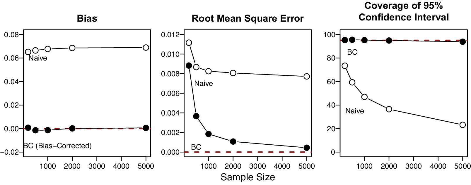
Figure 2 Finite sample performance of the naïve and bias-corrected estimators. Note: This figure displays the bias, root-mean-square error, and the coverage of the 95% confidence interval of the naïve and bias-corrected estimators. The bias-corrected estimator is unbiased and consistent and has an ideal level of coverage.
The recent survey literature suggests that researchers be cautious when inattentive respondents have different outcome profiles (e.g., political interest) than attentive respondents (Alvarez et al. Reference Alvarez, Atkeson, Levin and Li2019; Berinsky et al. Reference Berinsky, Margolis and Sances2014). Paying attention to this issue is especially important when dealing with sensitive questions, since respondents who have sensitive attributes may be more likely to give random answers than other respondents. To investigate whether our correction is robust to such an association, we replicate our simulations in Figure 1 by varying the prevalence of sensitive attributes among inattentive respondents while holding the prevalence among attentive respondents constant. Figure 3 shows that our bias-corrected estimator properly captures the true prevalence rate of sensitive attributes regardless of the degree of association between inattentiveness and possession of sensitive attributes. In contrast, the naïve estimator does not capture the ground truth when more than about 10% of respondents are inattentive. More simulation results are reported in Online Appendix B.

Figure 3 When respondents with sensitive attributes tend to be more inattentive. Note: This graph illustrates the naïve and bias-corrected estimators with 95% confidence intervals when the prevalence of sensitive attributes among inattentive respondents (
 $\pi _{\text {inattentive}}$
) is higher than that among attentive respondents (
$\pi _{\text {inattentive}}$
) is higher than that among attentive respondents (
 $\pi _{\text {attentive}}$
) with simulated data (see the top-middle panel for parameter values). Each panel is based on our simulation in which we set the number of respondents
$\pi _{\text {attentive}}$
) with simulated data (see the top-middle panel for parameter values). Each panel is based on our simulation in which we set the number of respondents
 $n=2,000$
, the proportion of a sensitive anchor item
$n=2,000$
, the proportion of a sensitive anchor item
 $\pi '=0$
, the proportions for nonsensitive items in the crosswise and anchor questions
$\pi '=0$
, the proportions for nonsensitive items in the crosswise and anchor questions
 $p=0$
and
$p=0$
and
 $p'=0$
, respectively. The bias-corrected estimator captures the ground truth (dashed line) even when respondents with sensitive attributes tend to be more inattentive.
$p'=0$
, respectively. The bias-corrected estimator captures the ground truth (dashed line) even when respondents with sensitive attributes tend to be more inattentive.
5 Extensions of the Bias-Corrected Estimator
5.1 Sensitivity Analysis
While our bias-corrected estimator requires the anchor question, it may not always be available. For such surveys, we propose a sensitivity analysis that shows researchers the sensitivity of their naïve estimates to inattentive respondents and what assumptions they must make to preserve their original conclusions. Specifically, it offers sensitivity bounds for original crosswise estimates by applying the bias correction under varying levels of inattentive respondents. To illustrate, we attempted to apply our sensitivity analysis to all published crosswise studies of sensitive behaviors from 2008 to the present (49 estimates reported in 21 original studies). Figure 4 visualizes the sensitivity bounds for selected studies (see Online Appendix C.1 for full results). For each study, we plot the bias-corrected estimates against varying percentages of inattentive respondents under Assumption 1. Our sensitivity analysis suggests that many studies would not find any statistically significant difference between direct questioning and the crosswise model (echoing Höglinger and Diekmann Reference Höglinger and Diekmann2017, 135) unless they assume that less than 20% of the respondents were inattentive.Footnote 16

Figure 4 Sensitivity analysis of previous crosswise estimates. Note: This figure plots bias-corrected estimates of the crosswise model over varying percentages of inattentive respondents with the estimate based on direct questioning reported in each study.
5.2 Weighting
While the literature on the crosswise model usually assumes that survey respondents are drawn from a finite target population via simple random sampling with replacement, a growing share of surveys are administered with unrepresentative samples such as online opt-in samples (Franco et al. Reference Franco, Malhotra, Simonovits and Zigerell2017; Mercer, Lau, and Kennedy Reference Mercer, Lau and Kennedy2018). Online opt-in samples are known to be often unrepresentative of the entire population that researchers want to study (Bowyer and Rogowski Reference Bowyer and Rogowski2017; Malhotra and Krosnick Reference Malhotra and Krosnick2007), and analysts using such samples may wish to use weighting to extend their inferences into the population of real interest. In this light, we propose a simple way to include sample weights in the bias-corrected estimator. Online Appendix C.2 presents our theoretical and simulation results. The key idea is that we can apply a Horvitz–Thompson-type estimator (Horvitz and Thompson Reference Horvitz and Thompson1952) to the observed proportions in the crosswise and anchor questions (for a similar result without bias correction, see Chaudhuri (Reference Chaudhuri2012, 380) and Quatember (Reference Quatember2019, 270)).
5.3 Multivariate Regressions for the Crosswise Model
Political scientists often wish to not only estimate the prevalence of sensitive attributes (e.g., corruption in a legislature), but also analyze what kinds of individuals (e.g., politicians) are more likely to have the sensitive attribute and probe whether having the sensitive attribute is associated with another outcome (e.g., reelection). In this vein, regression models for the traditional crosswise model have been proposed in several studies (Gingerich et al. Reference Gingerich, Oliveros, Corbacho and Ruiz-Vega2016; Jann et al. Reference Jann, Jerke and Krumpal2012; Korndörfer, Krumpal, and Schmukle Reference Korndörfer, Krumpal and Schmukle2014; Vakilian, Mousavi, and Keramat Reference Vakilian, Mousavi and Keramat2014). Our contribution is to further extend such a framework by (1) enabling analysts to use the latent sensitive attribute both as an outcome and a predictor while (2) applying our bias correction. Our software can easily implement these regressions while also offering simple ways to perform post-estimation simulation (e.g., generating predicted probabilities with 95% confidence intervals).
We first introduce multivariate regressions in which the latent variable for having a sensitive attribute is used as an outcome variable. Let
 $Z_{i}\in \{0,1\}$
be a binary variable denoting if respondent i has a sensitive attribute and
$Z_{i}\in \{0,1\}$
be a binary variable denoting if respondent i has a sensitive attribute and
 $T_{i}\in \{0,1\}$
be a binary variable denoting if the same respondent is attentive. Both of these quantities are unobserved latent variables. We define the regression model (conditional expectation) of interest as:
$T_{i}\in \{0,1\}$
be a binary variable denoting if the same respondent is attentive. Both of these quantities are unobserved latent variables. We define the regression model (conditional expectation) of interest as:
 $$ \begin{align} \mathbb{E}[Z_{i}|\textbf{X}_{\textbf{i}}=\textbf{x}] = \mathbb{P}(Z_{i}=1|\textbf{X}_{\textbf{i}}=\textbf{x}) = \pi_{\boldsymbol{\beta}}(\textbf{x}), \end{align} $$
where
 $\textbf {X}_{\textbf{i}}$
is a random vector of respondent i’s characteristics,
$\textbf {X}_{\textbf{i}}$
is a random vector of respondent i’s characteristics,
 $\textbf {x}$
is a vector of realized values of such covariates, and
$\textbf {x}$
is a vector of realized values of such covariates, and
 $\boldsymbol {\beta }$
is a vector of unknown parameters that associate these characteristics with the probability of having the sensitive attribute. Our goal is to make inferences about these unknown parameters and to use estimated coefficients to produce predictions.
$\boldsymbol {\beta }$
is a vector of unknown parameters that associate these characteristics with the probability of having the sensitive attribute. Our goal is to make inferences about these unknown parameters and to use estimated coefficients to produce predictions.
To apply our bias correction, we also introduce the following conditional expectation for being attentive:
 $$ \begin{align} \mathbb{E}[T_{i}|\textbf{X}_{\textbf{i}}=\textbf{x}] = \mathbb{P}(T_{i}=1|\textbf{X}_{\textbf{i}}=\textbf{x}) = \gamma_{\boldsymbol{\theta}}(\textbf{x}), \end{align} $$
where
 $\boldsymbol {\theta }$
is a vector of unknown parameters that associate the same respondent’s characteristics with the probability of being attentive. We then assume that
$\boldsymbol {\theta }$
is a vector of unknown parameters that associate the same respondent’s characteristics with the probability of being attentive. We then assume that
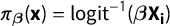 $\pi _{\boldsymbol {\beta }}(\textbf {x}) = \text {logit}^{-1}(\boldsymbol {\beta } \textbf {X}_{\textbf{i}})$
and
$\pi _{\boldsymbol {\beta }}(\textbf {x}) = \text {logit}^{-1}(\boldsymbol {\beta } \textbf {X}_{\textbf{i}})$
and
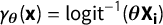 $\gamma _{\boldsymbol {\theta }}(\textbf {x}) = \text {logit}^{-1}(\boldsymbol {\theta } \textbf {X}_{\textbf{i}})$
, acknowledging that other functional forms are also possible.
$\gamma _{\boldsymbol {\theta }}(\textbf {x}) = \text {logit}^{-1}(\boldsymbol {\theta } \textbf {X}_{\textbf{i}})$
, acknowledging that other functional forms are also possible.
Next, we substitute these quantities into Equation (1c) by assuming
 $\pi '=0$
(zero-prevalence for Statement C):
$\pi '=0$
(zero-prevalence for Statement C):
 $$ \begin{align} \lambda_{\boldsymbol{\beta,\theta}}(\textbf{X}_{\textbf{i}}) & = \underbrace{\Big(\pi_{\boldsymbol{\beta}}(\textbf{X}_{\textbf{i}}) p + (1-\pi_{\boldsymbol{\beta}}(\textbf{X}_{\textbf{i}}))(1-p)\Big) \gamma_{\boldsymbol{\theta}}(\textbf{X}_{\textbf{i}}) + \frac{1}{2}\Big(1-\gamma_{\boldsymbol{\theta}}(\textbf{X}_{\textbf{i}})\Big)}_{\text{Conditional probability of choosing "both or neither is true" in the crosswise question}}, \end{align} $$
 $$ \begin{align} \lambda^{\prime}_{\boldsymbol{\theta}}(\textbf{X}_{\textbf{i}}) & = \underbrace{ \Big( \frac{1}{2}-p' \Big)\gamma_{\boldsymbol{\theta}}(\textbf{X}_{\textbf{i}}) + \frac{1}{2}}_{\text{Conditional probability of choosing "both or neither is true" in the anchor question}}. \end{align} $$
Finally, let
 $Y_{i}\in \{0,1\}$
and
$Y_{i}\in \{0,1\}$
and
 $A_{i}\in \{0,1\}$
be observed variables denoting if respondent i chooses “both or neither is true” in the crosswise and anchor questions, respectively. Assuming
$A_{i}\in \{0,1\}$
be observed variables denoting if respondent i chooses “both or neither is true” in the crosswise and anchor questions, respectively. Assuming
 $Y_{i}\mathop {\perp \!\!\!\!\perp } A_{i}|\textbf {X}_{\textbf{i}}$
with Assumptions 1–3, we model that
$Y_{i}\mathop {\perp \!\!\!\!\perp } A_{i}|\textbf {X}_{\textbf{i}}$
with Assumptions 1–3, we model that
 $Y_{i}$
and
$Y_{i}$
and
 $A_{i}$
follow independent Bernoulli distributions with success probabilities
$A_{i}$
follow independent Bernoulli distributions with success probabilities
 $\lambda _{\boldsymbol {\beta ,\theta }}(\textbf {X}_{\textbf{i}})$
and
$\lambda _{\boldsymbol {\beta ,\theta }}(\textbf {X}_{\textbf{i}})$
and
 $\lambda ^{\prime }_{\boldsymbol {\theta }}(\textbf {X}_{\textbf{i}})$
and construct the following likelihood function:
$\lambda ^{\prime }_{\boldsymbol {\theta }}(\textbf {X}_{\textbf{i}})$
and construct the following likelihood function:
 $$ \begin{align} \mathcal{L}(\boldsymbol{\beta}, \boldsymbol{\theta}|\{\textbf{X}_{\textbf{i}}, Y_{i}, A_{i}\}_{i=1}^{n}, p, p') & \propto \prod_{i=1}^{n} \Big\{ \lambda_{\boldsymbol{\beta,\theta}}(\textbf{X}_{\textbf{i}}) \Big\}^{Y_{i}} \Big\{ 1 - \lambda_{\boldsymbol{\beta,\theta}}(\textbf{X}_{\textbf{i}}) \Big\}^{1-Y_{i}} \Big\{ \lambda^{\prime}_{\boldsymbol{\theta}}(\textbf{X}_{\textbf{i}}) \Big\}^{A_{i}}\Big\{ 1 - \lambda^{\prime}_{\boldsymbol{\theta}}(\textbf{X}_{\textbf{i}}) \Big\}^{1 - A_{i}}\nonumber\\ & = \prod_{i=1}^{n} \Big\{ \Big(\pi_{\boldsymbol{\beta}}(\textbf{X}_{\textbf{i}}) p + (1-\pi_{\boldsymbol{\beta}}(\textbf{X}_{\textbf{i}}))(1-p)\Big) \gamma_{\boldsymbol{\theta}}(\textbf{X}_{\textbf{i}}) + \frac{1}{2}\Big(1-\gamma_{\boldsymbol{\theta}}(\textbf{X}_{\textbf{i}})\Big) \Big\}^{Y_{i}}\nonumber\\ & \quad \ \ \ \times \Big\{ 1 - \Big[\Big(\pi_{\boldsymbol{\beta}}(\textbf{X}_{\textbf{i}}) p + (1-\pi_{\boldsymbol{\beta}}(\textbf{X}_{\textbf{i}}))(1-p)\Big) \gamma_{\boldsymbol{\theta}}(\textbf{X}_{\textbf{i}}) + \frac{1}{2}\Big(1-\gamma_{\boldsymbol{\theta}}(\textbf{X}_{\textbf{i}})\Big) \Big] \Big\}^{1-Y_{i}}\nonumber\\ & \quad \ \ \ \times \Big\{ \Big( \frac{1}{2}-p' \Big)\gamma_{\boldsymbol{\theta}}(\textbf{X}_{\textbf{i}}) + \frac{1}{2} \Big\}^{A_{i}}\nonumber\\ & \quad \ \ \ \times \Big\{ 1 - \Big[ \Big( \frac{1}{2}-p' \Big)\gamma_{\boldsymbol{\theta}}(\textbf{X}_{\textbf{i}}) + \frac{1}{2} \Big] \Big\}^{1 - A_{i}}\nonumber\\ & = \prod_{i=1}^{n} \Big\{ \Big((2p-1)\pi_{\boldsymbol{\beta}}(\textbf{X}_{\textbf{i}}) + \Big(\frac{1}{2}-p \Big)\Big) \gamma_{\boldsymbol{\theta}}(\textbf{X}_{\textbf{i}}) + \frac{1}{2} \Big\}^{Y_{i}}\nonumber\\ & \quad \ \ \ \times \Big\{ 1 - \Big[ \Big((2p-1)\pi_{\boldsymbol{\beta}}(\textbf{X}_{\textbf{i}}) + \Big(\frac{1}{2}-p \Big)\Big) \gamma_{\boldsymbol{\theta}}(\textbf{X}_{\textbf{i}}) + \frac{1}{2} \Big] \Big\}^{1-Y_{i}}\nonumber\\ & \quad \ \ \ \times \Big\{ \Big( \frac{1}{2}-p' \Big)\gamma_{\boldsymbol{\theta}}(\textbf{X}_{\textbf{i}}) + \frac{1}{2} \Big\}^{A_{i}}\nonumber\\ & \quad \ \ \ \times \Big\{ 1 - \Big[ \Big( \frac{1}{2}-p' \Big)\gamma_{\boldsymbol{\theta}}(\textbf{X}_{\textbf{i}}) + \frac{1}{2} \Big] \Big\}^{1 - A_{i}}. \end{align} $$
Our simulations show that estimating the above model can recover both primary (
 $\boldsymbol {\beta }$
) and auxiliary parameters (
$\boldsymbol {\beta }$
) and auxiliary parameters (
 $\boldsymbol {\theta }$
) (Online Appendix C.3). Online Appendix C.4 presents multivariate regressions in which the latent variable for having a sensitive attribute is used as a predictor.
$\boldsymbol {\theta }$
) (Online Appendix C.3). Online Appendix C.4 presents multivariate regressions in which the latent variable for having a sensitive attribute is used as a predictor.
5.4 Sample Size Determination and Parameter Selection
When using the crosswise model with our procedure, researchers may wish to choose the sample size and specify other design parameters (i.e.,
 $\pi '$
, p, and
$\pi '$
, p, and
 $p'$
) so that they can obtain (1) high statistical power for hypothesis testing and/or (2) narrow confidence intervals for precise estimation. To fulfill these needs, we develop power analysis and data simulation tools appropriate for our bias-corrected estimator (Online Appendix C.5).
$p'$
) so that they can obtain (1) high statistical power for hypothesis testing and/or (2) narrow confidence intervals for precise estimation. To fulfill these needs, we develop power analysis and data simulation tools appropriate for our bias-corrected estimator (Online Appendix C.5).
6 Concluding Remarks
The crosswise model is a simple but powerful survey-based tool for investigating the prevalence of sensitive attitudes and behavior. To overcome two limitations of the design, we proposed a simple design-based solution using an anchor question. We also provided several extensions of our proposed bias-corrected estimator. Future research could further extend our methodology by applying it to nonbinary sensitive questions, allowing for multiple sensitive statements and/or anchor questions, handling missing data more efficiently, and integrating our method with more efficient sampling schemes (e.g., Reiber, Schnuerch, and Ulrich Reference Reiber, Schnuerch and Ulrich2020).
With these developments, we hope to facilitate the wider adoption of the (bias-corrected) crosswise model in political science, as it may have several advantages over traditional randomized response techniques, list experiments, and endorsement experiments. Future research should also explore how to compare and combine results from the crosswise model and these other techniques.
Our work also speaks to recent scholarship on inattentive respondents in self-administered surveys. While it is increasingly common for political scientists to use self-administered surveys, the most common way of dealing with inattentive respondents is to try to directly identify them through “screener”-type questions. However, a growing number of respondents are experienced survey-takers who may recognize and avoid such “traps” (Alvarez et al. Reference Alvarez, Atkeson, Levin and Li2019). Our method is one example of a different approach to handling inattentive respondents that is less likely to be recognized by respondents, works without measuring individual-level inattentiveness, and does not need to drop inattentive respondents from the sample. Future research should explore whether a similar approach to inattention would work in other question formats.
Acknowledgments
The previous version of this manuscript was titled as “Bias-Corrected Crosswise Estimators for Sensitive Inquiries.” For helpful comments and valuable feedback, we would like to thank Graeme Blair, Gustavo Guajardo, Dongzhou Huang, Colin Jones, Gary King, Shiro Kuriwaki, Jeff Lewis, John Londregan, Yui Nishimura, Michelle Torres, and three anonymous reviewers.
Data Availability Statement
Replication code for this article is available at https://doi.org/10.7910/DVN/AHWMIL (Atsusaka and Stevenson Reference Atsusaka and Stevenson2021). An open-source software R package cWise: A (Cross)Wise Method to Analyze Sensitive Survey Questions, which implements our methods, is available at https://github.com/YukiAtsusaka/cWise.
Supplementary Material
For supplementary material accompanying this paper, please visit https://doi.org/10.1017/pan.2021.43.


 Open access