


1. Introduction
Signed networks, in which positive and negative ties denote cooperative and conflictual interactions respectively, are a natural framework in which to represent militarized politics such as international relations and civil wars. Structural balance theory, which assumes that realpolitik maxims such as “the enemy of my enemy is my friend” are paramount in tie formation, has been the focus of applications of signed networks to international relations. This research has mostly involved tests of whether structural balance characterizes the structure of observed networks of alliances and clashes between nations (Maoz et al., Reference Maoz, Terris, Kuperman and Talmud2007; Lerner, Reference Lerner2016; Kirkley et al., Reference Kirkley, Cantwell and Newman2019). However, fundamental questions involving the dynamics of signed international relations have been neglected, such as how do feedbacks from competing mechanisms act to stabilize or destabilize the system leading to transitions between peace and war; what patterns of alliances and rivalries may be more susceptible to destabilization; and how does the system respond to perturbations such as the flare-up of hostilities between particular countries. Models of signed network dynamics in which network tie values evolve under their mutual influence, such as the one we present here, can help illuminate such questions.
Although the most straightforward dynamical formulation of structural balance theory with continuous tie values has been successful in showing how different outcomes predicted by the theory can arise from initial conditions (Kulakowski et al., Reference Kulakowski, Gawronski and Gronek2005; Marvel et al., Reference Marvel, Kleinberg, Kleinberg and Strogatz2011; Morrison & Gabbay, Reference Morrison and Gabbay2020), the intent to faithfully encode structural balance theory saddles it with significant conceptual and mathematical shortcomings, limiting the ability to yield a richer and more realistic range of behaviors. The assumption that changes in tie strength between a pair of nodes are determined only by their relations with third parties ignores dyad-specific drivers of rivalry or friendship due, for instance, to territorial disputes or ideological similarities or differences. This neglect of potentially countervailing processes implies that even if the initial tie magnitudes are small, they will be amplified toward a balanced end state of either systemic two-faction war or complete network harmony, whereas the international system is typically characterized by more prosaic conditions of lower level conflict and cooperation. Furthermore, once the network evolves into a state consistent with structural balance, it will stay there forever. Consequently, the absence of competing mechanisms implies that a model of pure structural balance cannot address how a system transitions from peace to war, or back again, as key conditions of the international system such as the balance of power change. Moreover, the structural balance force in the simple model is not bounded, generating infinite tie values of unlimited affinity or animosity.
We introduce a dynamical systems model of signed network evolution that includes, along with structural balance, a force that models direct dyadic interaction, thereby enabling it to capture transitions between systemic peace and systemic war, where “systemic” refers to most, if not all, of the nodes in the network. This direct dyadic force acts so as to pull a dyad toward a dyad-specific tie value parameter, known as the “dyadic bias,” taken to represent their level of amicable or contentious relations while at peace. When structural balance pressures are absent or weak, the equilibrium tie value will be at or near the dyadic bias parameter. Along with incorporating this dyadic force, we modify the form of the structural balance force itself so that its strength saturates as mutual allies (or enemies) predominate rather than growing without bound.
Our model can display sharp transitions between the different equilibria corresponding to peace and war. These transitions occur via a bifurcation which is a sudden change in the qualitative nature of the solution space as a model parameter is varied (Strogatz & Dichter, Reference Strogatz and Dichter2016). As the parameter controlling the structural balance force increases, the system exhibits a bifurcation from the systemic peace state to the systemic war state. An increase in the “structural balance sensitivity” parameter reflects a systemic change in a sociopolitical network that impels nodes to increasingly take mutual allies or enemies into account in their relations with others. For the international system, this increased sensitivity to the network structure may be due to a narrowing power gap in a rivalry between the dominant state and a rising challenger or technological developments perceived as favoring offense over defense, factors theorized as causes of major wars (Van Evera, Reference Van1999; Copeland, Reference Copeland2000). The reverse transition from war to peace is also possible but occurs at a different and lower structural balance sensitivity value. This phenomenon, known as hysteresis, reflects the underlying bistability of the system in a certain parameter regime. The capability to account for both peace-to-war and war-to-peace transitions distinguishes our model from many dynamics models which only address conflict onset.
We investigate the bifurcation behavior of our model in simulations and use stability analysis to derive expressions relating to system parameters at the critical points where bifurcations occur. We do so for both a special case that can be reduced to a one-dimensional system and the general case involving matrix formalism. Spectral decomposition of the system of tie values evolved by the model (the “dynamic network”) into eigenvalues and eigenvectors proves to be a useful tool for illuminating the model behavior in simulations. It is also crucial in the stability analysis as the bifurcations between peace and war are manifested as discontinuities in the first eigenvalue of the matrix of dyadic biases (the “bias network”).
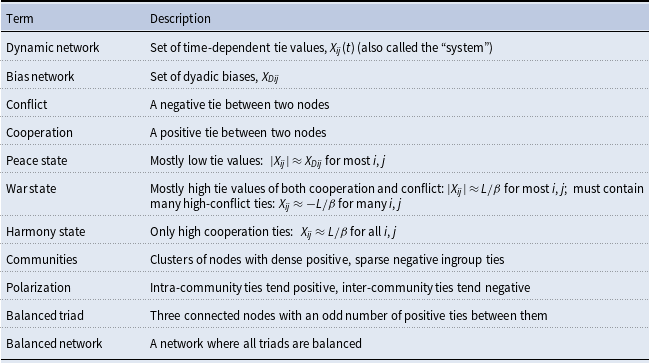
Community structure—tie density patterns that allow for node clustering—can be built into the bias network; polarized community structure can be generated via a two-block structure where intra-block biases tend to be positive and inter-block ones tend to be negative (Table 1). Simulations show that the peace-to-war bifurcation occurs at a lower structural balance sensitivity for networks with polarized community structure characterized by opposing factions than those without such structure. The stability analysis reveals the mathematical underpinnings of this effect: the structural balance sensitivity at which the peace-to-war bifurcation occurs decreases in inverse proportion to the first eigenvalue of the matrix of dyadic bias parameters, which is larger for the polarized structure case. We use this result to argue more generally that polarized community structure, in which hostile factions have a discernible signature in the eigenvalue spectrum, will be more unstable to war than the case where the structure is disordered. As heightened polarization between two rival alliances has been attributed as a cause of greater instability to systemic war (Thompson, Reference Thompson2003), our analysis therefore explains how this behavior can emerge naturally from signed network dynamics and generalizes it beyond the context of formal alliances.
Table 1. Summary of select network terms
Another aspect of our results bears upon the question of whether particular dyads are more destabilizing than others in terms of catalyzing major war (Thompson, Reference Thompson2003). Standard stability analysis, as employed in obtaining the results noted above, assumes a perspective in which a parameter change causes an equilibrium to become unstable to even infinitesimal perturbations in tie values. However, it is also possible to consider how finite perturbations, such as increased cooperation or conflict among certain dyads, may destabilize the system, while keeping model parameters fixed. This can occur in the bistable state where both the peace and war states are stable and so the dynamic network will remain at its present equilibrium unless shaken out to the other one. We define an optimization framework which seeks to find the perturbation that can trigger such a transition with the least “energy” in terms of the change in network tie values from their present state. We illustrate this framework using a simplified World War I context consisting of empirical networks of five great powers. We find that the ties that triggered the war require relatively low energy to destabilize the system.
We also illustrate how the response of the dynamic network to perturbations changes as the system nears the bifurcation point. In particular, the duration of the transient caused by the perturbation becomes longer in a power-law relationship universal to all systems that undergo a saddle-node bifurcation, as our model does, in a phenomenon known as “critical slowing down” (Kuehn, Reference Kuehn2011). The universality implies that critical slowing down may be useful as an early warning signal for detecting impending major state transitions in complex systems, such as the climate, ecosystems, and social systems, for which precise dynamical models are unavailable (Scheffer et al., Reference Scheffer, Carpenter, Lenton, Bascompte, Brock, Dakos and Vandermeer2012).
Our signed network modeling approach integrates the nonlinear dynamics of complex systems (Strogatz & Dichter, Reference Strogatz and Dichter2016; Roberts, Reference Roberts2015) with the rich, quantitative representation of structure in complex networks (Newman, Reference Newman2018; Doreian et al., Reference Doreian, Batagelj and Ferligoj2020). Accordingly, it meshes two strands of international relations research: one which casts world politics as a complex system where nonlinear feedback between system components can cause disproportional and dramatic responses to small changes (Saperstein, Reference Saperstein1999; Jervis, Reference Jervis1997; Thompson, Reference Thompson2003; Ferguson, Reference Ferguson2010; Stauffer, Reference Stauffer2021) and the other which studies international relations with the concepts and methods of network analysis (Maoz, Reference Maoz2011; Dorussen et al., Reference Dorussen, Gartzke and Westerwinter2016). The system of alliances and rivalries among states has received much attention as a cause of systemic war (Snyder, Reference Snyder1984; Rasler & Thompson, Reference Rasler and Thompson2010; Levy & Mulligan, Reference Levy and Mulligan2021) and our model can shed light on which patterns are particularly prone to instability, as we will illustrate by our investigation of how the peace-to-war bifurcation is affected by polarized community structure and in our application to World War I. The analytical expressions for the bifurcation conditions we derive below will greatly facilitate more generalized study of the effects of different types of community structure, both abstract and empirical, by eliminating the need to identify bifurcation points through computationally intensive parameter sweeps of model simulations. And our finding that the interplay of the direct dyadic and structural balance forces generates a saddle-node bifurcation can guide future efforts to use universal phenomena such as critical slowing down as predictive indicators of conflict.
2. Background
2.1 Dynamical systems modeling and structural balance theory in international relations
Dynamical systems models have been useful in understanding and predicting the dynamics of complex systems in a diversity of fields such as biology, engineering, and sociology (Strogatz & Dichter, Reference Strogatz and Dichter2016). While statistical models are useful in classifying and predicting phenomena, statistical models often fail to provide explicit mechanistic explanations (Midlarsky, Reference Midlarsky1984; Thompson, Reference Thompson1986; Roberts et al., Reference Roberts, Augustine, Lawton, Lindsay, Thiele, Izquierdo and Lockery2016); dynamical systems models, on the other hand, can elucidate the mechanisms responsible for the observed underlying phenomena (Trotta et al., Reference Trotta, Bullinger and Sepulchre2012; Morrison & Kutz, Reference Morrison and Kutz2021). Dynamical systems models of the interaction between states or armed sub-state actors such as insurgents can help identify mechanisms for system destabilization as well as mechanisms for reinforcing stability. These models can be used to determine the risk for minor, localized conflicts to escalate and spread extensively to other nodes in the network. Moreover, they provide a rich set of diagnostic tools for the analysis of escalating conflicts which result in the outbreak of widespread wars.
The application of dynamical systems modeling to international relations has largely been built upon Richardson’s pioneering model of arms races (Gleditsch, Reference Gleditsch2020; Stauffer, Reference Stauffer2021). However, this stream of research predated the surge of scholarship on political networks and so did not engage with questions of network structure, although the Richardson model itself is amenable to network formulation (Ward, Reference Ward2020). Nor did it leverage the concepts and tools of modern bifurcation theory.
The application of network analysis to international relations has bloomed over the past two decades. Most of this work has involved unsigned networks in which either cooperative or, less frequently, conflictual ties are treated as separate networks between nations or militant groups (Hafner-Burton et al., Reference Hafner-Burton, Kahler and Montgomery2009; Maoz, Reference Maoz2011; Victor et al., Reference Victor, Montgomery and Lubell2016; Dorussen et al., Reference Dorussen, Gartzke and Westerwinter2016; Zech & Gabbay, Reference Zech and Gabbay2016). Signed networks, however, allow for an integration of cooperation and conflict consistent with the fact that alliances are usually formed with an eye toward a potential foe and decisions to militarily confront an opponent typically consider who might come to its aid. The investigation of world politics using signed networks has overwhelmingly been through the lens of structural balance theory (Cartwright & Harary, Reference Cartwright and Harary1956), a strand of research that precedes by decades the recent network turn in international relations study.
In its basic form, structural balance theory is formulated on (undirected) triads and asserts that there are only two balanced, and hence enduring, triads: one with all positive ties (“the friend of my friend is my friend”) and one with a single positive tie and two negative ones (“the enemy of my enemy is my friend”). The two other possibilities—two positive ties and one negative or three negative ties—are imbalanced and hence unstable. A network as a whole is considered balanced if it is comprised of only balanced triads. These rules imply that a complete network can have only two perfectly balanced states: a harmonious state in which all ties are positive and the two hostile factions state in which the ties within a faction are positive while the ties between factions are negative (Cartwright & Harary, Reference Cartwright and Harary1956).
There has been a long-running back-and-forth about whether the international system is characterized by structural balance (Harary, Reference Harary1961; Healy & Stein, Reference Healy and Stein1973; McDonald & Rosecrance, Reference McDonald and Rosecrance1985; Maoz et al., Reference Maoz, Terris, Kuperman and Talmud2007) with more recent work tending to support an overall tendency toward balance (Lerner, Reference Lerner2016; Kirkley et al., Reference Kirkley, Cantwell and Newman2019; Burghardt & Maoz, Reference Burghardt and Maoz2020). Going beyond the question of whether the international system displays a tendency toward balance, its level of balance has been observed to fluctuate considerably over time (Doreian & Mrvar, Reference Doreian and Mrvar2019; Burghardt & Maoz, Reference Burghardt and Maoz2020), which suggests that other forces beyond structural balance may be at work. Evidence for structural balance processes has also been found in friendship networks (Kirkley et al., Reference Kirkley, Cantwell and Newman2019), wild mammals (Ilany et al., Reference Ilany, Barocas, Koren, Kam and Geffen2013), and gang networks where inter-gang violence increases among gangs in imbalanced triads (Nakamura et al., Reference Nakamura, Tita and Krackhardt2020).
2.2 Modeling structural balance dynamics
Given a network of initial ties, dynamical systems models can be formulated that evolve ties over time consistent with structural balance theory. The simplest formulation of structural balance dynamics evolves a symmetric network of signed edge weights, $\textbf{X}(t) \in \mathbb{R}^{N \times N}$
, as the following system of coupled, nonlinear differential equations:
$\textbf{X}(t) \in \mathbb{R}^{N \times N}$
, as the following system of coupled, nonlinear differential equations:
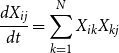 \begin{align} \frac{dX_{ij}}{dt} = \sum _{k=1}^N X_{ik}X_{kj} \end{align}
If nodes $i$
and
$i$
and $j$
have either both positive ties or both negative ties with a third node
$j$
have either both positive ties or both negative ties with a third node $k$
, the product
$k$
, the product $X_{ik}X_{kj}$
will be positive and act so as to increase their tie value
$X_{ik}X_{kj}$
will be positive and act so as to increase their tie value $X_{ij}$
. In contrast, if their ties with
$X_{ij}$
. In contrast, if their ties with $k$
are of opposite sign, the effect will be to decrease
$k$
are of opposite sign, the effect will be to decrease $X_{ij}$
. Both of these effects act to increase the balance in the system. The sum determines whether the net effect of all mutual ties increases or decreases
$X_{ij}$
. Both of these effects act to increase the balance in the system. The sum determines whether the net effect of all mutual ties increases or decreases $X_{ij}$
.
$X_{ij}$
.
Although this equation appears to have been first proposed by Lee et al. (Reference Lee, Muncaster and Zinnes1994), it was not investigated in that paper. It was proposed independently by Kulakowski et al. (Reference Kulakowski, Gawronski and Gronek2005) who found that in simulations this model leads to perfectly balanced outcomes consistent with the static theory. Marvel et al. (Reference Marvel, Kleinberg, Kleinberg and Strogatz2011) used the matrix equation formulation of Equation (1),
 \begin{align} \frac{d\textbf{X}}{dt} = \textbf{X}^2 \end{align}
to obtain an analytical solution for $\textbf{X}(t)$
. They showed that the network will generically evolve into a balanced end state as determined by the eigenvector of the initial adjacency matrix
$\textbf{X}(t)$
. They showed that the network will generically evolve into a balanced end state as determined by the eigenvector of the initial adjacency matrix $\textbf{X}(0)$
having the most positive eigenvalue, which grows the fastest. If this first eigenvector consists of all positive components, then the system will evolve into the harmonious state. On the other hand, if the first eigenvector has components of both positive and negative sign, then the system will evolve into the two hostile factions state. Marvel et al. (Reference Marvel, Kleinberg, Kleinberg and Strogatz2011) used this model to show good agreement with the alliances which formed in World War II and the split of the Zachary karate club. Morrison & Gabbay (Reference Morrison and Gabbay2020) extended this model to initial conditions containing community structure generated by a two-block stochastic model. They found that phase transitions in the initial network structure determine whether the two final factions align with the block structure or instead have random memberships unrelated to the blocks or, alternatively, whether it is the harmonious state that emerges.
$\textbf{X}(0)$
having the most positive eigenvalue, which grows the fastest. If this first eigenvector consists of all positive components, then the system will evolve into the harmonious state. On the other hand, if the first eigenvector has components of both positive and negative sign, then the system will evolve into the two hostile factions state. Marvel et al. (Reference Marvel, Kleinberg, Kleinberg and Strogatz2011) used this model to show good agreement with the alliances which formed in World War II and the split of the Zachary karate club. Morrison & Gabbay (Reference Morrison and Gabbay2020) extended this model to initial conditions containing community structure generated by a two-block stochastic model. They found that phase transitions in the initial network structure determine whether the two final factions align with the block structure or instead have random memberships unrelated to the blocks or, alternatively, whether it is the harmonious state that emerges.
Equation (1) can be analyzed for the case of a directed network in which case the system evolves to four factions instead of two from random initial conditions (Veerman, Reference Veerman2018). It is also possible to define a variant model for directed networks that replaces $X_{ik}X_{kj}$
on the right-hand side of (1) with
$X_{ik}X_{kj}$
on the right-hand side of (1) with $X_{ik}X_{jk}$
, which can be shown to evolve into two factions for random initial conditions (Traag et al., Reference Traag, Dooren and Leenheer2013). Although our focus here is on deterministic dynamical systems, structural balance theory can also be implemented as a stochastic model (Antal et al., Reference Antal, Krapivsky and Redner2006).
$X_{ik}X_{jk}$
, which can be shown to evolve into two factions for random initial conditions (Traag et al., Reference Traag, Dooren and Leenheer2013). Although our focus here is on deterministic dynamical systems, structural balance theory can also be implemented as a stochastic model (Antal et al., Reference Antal, Krapivsky and Redner2006).
As we employ a control theory framework to investigate the patterns of network perturbations that are most destabilizing, we note some previous work applying control theory to structural balance. Gao & Wang, (Reference Gao and Wang2018) have investigated the origins of balancing forces with respect to nodal interactions and have considered how to control structural balance edge dynamics using node dynamics, with the assumption that the dynamics of nodes and edges are interdependent. Wongkaew et al. (Reference Wongkaew, Caponigro, Kułakowski and Borzì2015) have considered how to control structural balance dynamics by introducing a “leader” to the system, while Summers & Shames (Reference Summers and Shames2013) have evaluated the control abilities of existing nodes in a network by changing ties.
While the simple model of Equation (1) has yielded great insight into structural balance dynamics and will serve as the main point of departure, it also has important shortcomings. Although it is able to determine the outcomes that emerge from a network solely under structural balance dynamics, it has no equilibrium, evolving ties toward positive or negative infinity (and does so in finite time (Marvel et al., Reference Marvel, Kleinberg, Kleinberg and Strogatz2011)). Once the model is turned on, the network perforce evolves into a state of complete war or harmony and so it cannot capture the stable, pre-escalatory state which characterizes the international system for long stretches of time before and after systemic wars. Its empirical application therefore depends upon the assumption that structural balance dynamics are either off or on and so, while useful for predicting the composition of the opposing sides once the war starts, the model is silent about what patterns of relationships might set off such a war in the first place. Nor can the model describe de-escalation dynamics, from systemic war back to a peaceful state since it inherently seeks to increase balance. Accordingly, we aim to build upon the dynamical systems model of conflict escalation in Equation (1) to create a model that can manifest a wider range of behaviors in the international system—stability in a peaceful, low-conflict state, transitions to systemic war, and de-escalation.
3. Signed network model of cooperation and conflict dynamics
We present a model for signed network edge dynamics that incorporates two major forces: (1) a dyadic force that seeks to stabilize a dyad’s tie value at a low level of cooperation or conflict as determined by the particular history and context of their relationship and (2) a bounded structural balance force, rather than the unbounded force of Equation (1). In addition, we will allow for transient perturbations of particular tie values to allow for investigation of how conflict flare-ups or temporary cooperation may affect the stability of the whole system.
In our model, the dynamics governing the rate of change for edge $X_{ij}(t)$
between nodes
$X_{ij}(t)$
between nodes $i$
and
$i$
and $j$
in a network containing
$j$
in a network containing $N$
nodes is given by
$N$
nodes is given by
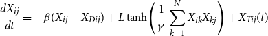 \begin{align} \frac{dX_{ij}}{dt} = -\beta (X_{ij} - X_{Dij}) + L \tanh \!\left ( \frac{1}{\gamma } \sum _{k=1}^N X_{ik}X_{kj} \right ) + X_{Tij}(t) \end{align}
where $-\beta (X_{ij} - X_{Dij})$
is the direct dyadic force,
$-\beta (X_{ij} - X_{Dij})$
is the direct dyadic force, $ L \tanh\!(\gamma ^{-1} \sum _{k=1}^N X_{ik}X_{kj})$
is the bounded structural balance term, and
$ L \tanh\!(\gamma ^{-1} \sum _{k=1}^N X_{ik}X_{kj})$
is the bounded structural balance term, and $X_{Tij}(t)$
represents fast-timescale perturbations. Although the above equation can be applied to directed networks, we will only consider the undirected case here so that
$X_{Tij}(t)$
represents fast-timescale perturbations. Although the above equation can be applied to directed networks, we will only consider the undirected case here so that $X_{ij}=X_{ji}$
. The other matrix quantities,
$X_{ij}=X_{ji}$
. The other matrix quantities, $X_{Dij}$
and
$X_{Dij}$
and $X_{Tij}$
, are similarly symmetric.
$X_{Tij}$
, are similarly symmetric.
The strength of the direct dyadic force is scaled by the parameter $\beta$
, which we take to be the same for all dyads.Footnote
1
We refer to
$\beta$
, which we take to be the same for all dyads.Footnote
1
We refer to $X_{Dij}$
as the dyadic bias parameter, which can take on dyad-specific values. Under the action of the direct dyadic force alone,
$X_{Dij}$
as the dyadic bias parameter, which can take on dyad-specific values. Under the action of the direct dyadic force alone, $X_{ij} \rightarrow X_{Dij}$
so that
$X_{ij} \rightarrow X_{Dij}$
so that $X_{Dij}$
is the equilibrium tie value. A weak structural balance force will cause only a small shift in the equilibrium values from the
$X_{Dij}$
is the equilibrium tie value. A weak structural balance force will cause only a small shift in the equilibrium values from the $X_{Dij}$
but, as will be seen, a sufficiently strong structural balance force will induce a transition to a high level of equilibrium tie values. The dyadic bias parameters will be taken to correspond to relatively low levels of cooperation and conflict (in comparison with wartime cooperation and conflict). There are many factors that can affect the propensity for two states to cooperate such as mutual trade interests or common ideology. Other factors such as common territorial aspirations or disparate ideologies predispose discordant states to hostility. We will typically, but not always, use the bias parameters as the initial tie values in our simulations,
$X_{Dij}$
but, as will be seen, a sufficiently strong structural balance force will induce a transition to a high level of equilibrium tie values. The dyadic bias parameters will be taken to correspond to relatively low levels of cooperation and conflict (in comparison with wartime cooperation and conflict). There are many factors that can affect the propensity for two states to cooperate such as mutual trade interests or common ideology. Other factors such as common territorial aspirations or disparate ideologies predispose discordant states to hostility. We will typically, but not always, use the bias parameters as the initial tie values in our simulations, $X_{ij}(0)=X_{Dij}$
.
$X_{ij}(0)=X_{Dij}$
.
The bounded form of the structural balance force is produced by the S-shaped hyperbolic tangent function, which asymptotes to $\pm L$
as its argument tends to
$\pm L$
as its argument tends to $\pm \infty$
.
$\pm \infty$
. $L$
therefore scales the maximum magnitude of the structural balance force. The parameter
$L$
therefore scales the maximum magnitude of the structural balance force. The parameter $\gamma$
is the characteristic half-width of the transition region between the negative and positive plateaus. It will be convenient for subsequent analysis to define the structural balance sensitivity,
$\gamma$
is the characteristic half-width of the transition region between the negative and positive plateaus. It will be convenient for subsequent analysis to define the structural balance sensitivity, $\alpha$
, which is the characteristic slope of the transition region,
$\alpha$
, which is the characteristic slope of the transition region, $\alpha =L/\gamma$
. In a small neighborhood around zero, the hyperbolic tangent is approximately linear so that the structural balance force is approximately given by
$\alpha =L/\gamma$
. In a small neighborhood around zero, the hyperbolic tangent is approximately linear so that the structural balance force is approximately given by $\alpha \sum _{k=1}^N X_{ik}X_{kj}$
and so reduces to the unbounded form of structural balance in Equation (1) in this neighborhood (apart from
$\alpha \sum _{k=1}^N X_{ik}X_{kj}$
and so reduces to the unbounded form of structural balance in Equation (1) in this neighborhood (apart from $\alpha$
, which is unnecessary in (1)). The strength of the balance force is also affected by the size of the network
$\alpha$
, which is unnecessary in (1)). The strength of the balance force is also affected by the size of the network $N$
and the tie density. Either increasing the size or the density of the network tends to increase
$N$
and the tie density. Either increasing the size or the density of the network tends to increase $\sum _{k=1}^N X_{ik}X_{kj}$
.
$\sum _{k=1}^N X_{ik}X_{kj}$
.
Saturation, as occurs in the structural balance force in our model, is a pervasive phenomena in natural systems. It appears in the dose-response curve in medicine and the saturation of information transfer in neuroscience (Calabrese, Reference Calabrese2016; Rioult-Pedotti et al., Reference Rioult-Pedotti, Friedman and Donoghue2000; Prescott & De Koninck, 2003). Saturation parameters appear due to bounds on acting and sensing. Saturation terms have been added to multi-agent models of nonlinear opinion dynamics in order to make the influence of opinion exchanges on agents more realistic (Bizyaeva et al., Reference Bizyaeva, Franci and Leonard2022; Franci et al., Reference Franci, Bizyaeva, Park and Leonard2021). Similar to other models of natural phenomena, we assume the network structure’s influence on ties saturates by bounding the structural balance term.
The term $X_{Tij}(t)$
contains transient perturbations to the system caused by fast-timescale events such as a militarized conflict between two states or cooperation against an adversary. It could take the form of an impulse, positive or negative, to a given dyad or a set of dyads. These impulses may knock the system out of its current equilibrium. Note that the
$X_{Tij}(t)$
contains transient perturbations to the system caused by fast-timescale events such as a militarized conflict between two states or cooperation against an adversary. It could take the form of an impulse, positive or negative, to a given dyad or a set of dyads. These impulses may knock the system out of its current equilibrium. Note that the $X_{Tij}(t)$
corresponds to finite perturbations as distinguished from the infinitesimal perturbations always assumed to be present and which prevent the system from staying in unstable equilibria.
$X_{Tij}(t)$
corresponds to finite perturbations as distinguished from the infinitesimal perturbations always assumed to be present and which prevent the system from staying in unstable equilibria.
We make a few remarks regarding the interpretation of the quantities in our model with specific respect to its application to transitions between systemic peace and war. First, we assume that the wartime levels of both conflict and cooperation are much larger than their peacetime values. Denoting war and peace respectively by the subscripts W and P, this assumption can be written mathematically as $|X_{Wij}| \gg |X_{Pij}|$
. We can enforce this assumption in the war and peace equilibria generated by the model by setting our parameter values such that
$|X_{Wij}| \gg |X_{Pij}|$
. We can enforce this assumption in the war and peace equilibria generated by the model by setting our parameter values such that $L/\beta \gg |X_{Dij}| \forall\ i,j$
. In the peace equilibrium, the tie values will be approximately given by their dyadic bias values,
$L/\beta \gg |X_{Dij}| \forall\ i,j$
. In the peace equilibrium, the tie values will be approximately given by their dyadic bias values, $X_{Pij} \approx X_{Dij}$
. Similarly, the war equilibrium tie values will be characterized by
$X_{Pij} \approx X_{Dij}$
. Similarly, the war equilibrium tie values will be characterized by $|X_{Wij}| \approx L/\beta$
. If we take
$|X_{Wij}| \approx L/\beta$
. If we take $\beta =1$
, then
$\beta =1$
, then $L$
can be interpreted simply as scaling wartime cooperation and conflict. There is a zone of tie values intermediate between these peace and war scales but they are only passed through transiently in the model. The magnitude of the leading eigenvalue of the dynamic network can be used to measure the network’s global state; increasing the magnitude of tie values increases the leading eigenvalue of the system.
$L$
can be interpreted simply as scaling wartime cooperation and conflict. There is a zone of tie values intermediate between these peace and war scales but they are only passed through transiently in the model. The magnitude of the leading eigenvalue of the dynamic network can be used to measure the network’s global state; increasing the magnitude of tie values increases the leading eigenvalue of the system.
Our distinction between low versus high conflict and/or cooperation levels is synonymous with this assumption of different scales for peace and war: low tie values have a magnitude at or below the scale set by the bias network and therefore are much lower than the high tie magnitudes characteristic of war. We say that the dynamic network as a whole is in a systemic “war state” if most, if not all, of the ties between countries are high-strength ties of both cooperation and conflict.Footnote 2 Note the presence of high cooperation in addition to conflict implies that the war state consists of warring alliances rather than simply an amalgamation of uncoupled dyadic wars. In the systemic “peace state,” most of the tie strengths are low, although there may be a few high-strength ties. This representation of peace along a spectrum of low-level conflict and cooperation is in the spirit of recent efforts to resolve peace in finer detail than simply the absence of war (Diehl, Reference Diehl2016).
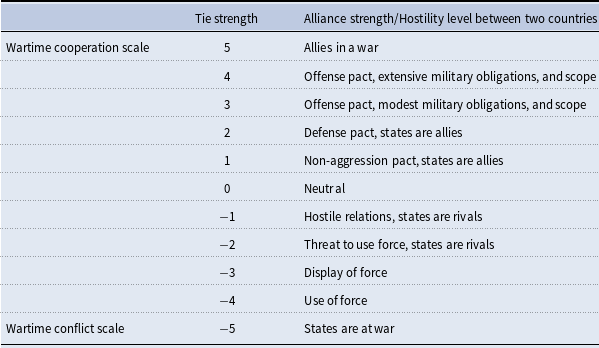
Alliance strengths between nations are coded using the extensiveness of the commitments that exist between them (Leeds et al., 2002; Gibler, Reference Gibler2009; Singer & Small, Reference Singer and Small1966), while rivalries are coded by the level of hostility, perceived threat, and force used between nations (Palmer et al., 2015; Thompson & Dreyer, Reference Thompson and Dreyer2011). Positive relations can range from ententes to extensive defense and offense pacts while negative relations can range from mild rivalries to uses of force and even war. Section 8 provides an example of how alliance strengths and hostility levels map onto network tie values in our model (Table 2).
Table 2. Network tie value meanings in terms of international relations
Our discussion on the bifurcations between the peace and war states below often centers around varying the structural balance sensitivity $\alpha$
and identifying the critical value of
$\alpha$
and identifying the critical value of $\alpha$
at which the bifurcation occurs. The above identification of the war state scale of high tie values,
$\alpha$
at which the bifurcation occurs. The above identification of the war state scale of high tie values, $|X_{Wij}| \approx L/\beta$
, helps provide a specific substantive interpretation of what varying
$|X_{Wij}| \approx L/\beta$
, helps provide a specific substantive interpretation of what varying $\alpha$
can signify. If we hold
$\alpha$
can signify. If we hold $L$
and
$L$
and $\beta$
constant, then we also fix the scale of wartime cooperation and conflict. Increasing
$\beta$
constant, then we also fix the scale of wartime cooperation and conflict. Increasing $\alpha$
is then equivalent to decreasing
$\alpha$
is then equivalent to decreasing $\gamma$
so that the transition region of the structural balance force curve becomes narrower, which implies that the tie value between a pair of countries becomes more sensitive to changes in their relationships with other countries (to which they are both connected).
$\gamma$
so that the transition region of the structural balance force curve becomes narrower, which implies that the tie value between a pair of countries becomes more sensitive to changes in their relationships with other countries (to which they are both connected).
In addition to the peace and war states, there is a third possible equilibrium in which all the network ties are high cooperation. We refer to this as the “harmony state.” Note that while the harmony state certainly is peaceful, we reserve the term peace state to refer to the more prosaic state of low-level cooperation and conflict that characterizes peace in the international system as defined above. Table 1 summarizes the key network terms and equilibrium states.
Lastly, we note that the dynamics of this model results in nonzero self-ties, $X_{ii}$
. These ties will always be positive because the structural balance term becomes a sum over
$X_{ii}$
. These ties will always be positive because the structural balance term becomes a sum over $X^2_{ik}$
(unless one makes the odd choice of a negative self-bias,
$X^2_{ik}$
(unless one makes the odd choice of a negative self-bias, $X_{Dii}\lt 0$
, implying that the node has a conflictual relationship with itself). Since it is not obvious how to empirically measure a self-tie, they are often set to zero and we do so in the dyadic bias matrix
$X_{Dii}\lt 0$
, implying that the node has a conflictual relationship with itself). Since it is not obvious how to empirically measure a self-tie, they are often set to zero and we do so in the dyadic bias matrix $\textbf{X}_D$
. Yet, conceptually, a positive self-tie is not problematic as it can be interpreted as self-cooperation. When a node is a composite entity such as a country, a high self-cooperation, for instance, could correspond to greater mobilization of the populace during a war. Whether or not the self-tie is set to zero would be simply a conceptual choice were it not for the fact that it does enter into the dynamics of the other ties,
$\textbf{X}_D$
. Yet, conceptually, a positive self-tie is not problematic as it can be interpreted as self-cooperation. When a node is a composite entity such as a country, a high self-cooperation, for instance, could correspond to greater mobilization of the populace during a war. Whether or not the self-tie is set to zero would be simply a conceptual choice were it not for the fact that it does enter into the dynamics of the other ties, $X_{ij}$
. In the roughly linear region of the hyperbolic tangent, the self-ties contribute a force
$X_{ij}$
. In the roughly linear region of the hyperbolic tangent, the self-ties contribute a force $\alpha (X_{ii} + X_{jj})X_{ij}$
, which has the effect of adding a nonlinear term to the direct dyadic force. Given the positivity of the self-ties, this self-ties force produces a tendency for a dyad to be further pushed in the direction of its present sign, toward more cooperation for
$\alpha (X_{ii} + X_{jj})X_{ij}$
, which has the effect of adding a nonlinear term to the direct dyadic force. Given the positivity of the self-ties, this self-ties force produces a tendency for a dyad to be further pushed in the direction of its present sign, toward more cooperation for $X_{ij}(t)\gt 0$
and more conflict if
$X_{ij}(t)\gt 0$
and more conflict if $X_{ij}(t)\lt 0$
, corresponding to mutually reinforcing behavior between the nodes in the dyad.Footnote
3
However, this self-ties contribution contains just two of
$X_{ij}(t)\lt 0$
, corresponding to mutually reinforcing behavior between the nodes in the dyad.Footnote
3
However, this self-ties contribution contains just two of $N$
terms appearing in the structural balance force and so becomes ever more negligible as the number of nodes grows larger.
$N$
terms appearing in the structural balance force and so becomes ever more negligible as the number of nodes grows larger.
4. Model behavior
In this section, we use simulations to explore the dynamics of the above model. The model shows a peace-to-war bifurcation as the structural balance sensitivity $\alpha$
is increased, which reflects the feed-forward escalatory conflict that spreads throughout the entire dynamic network, requiring each node to participate in the global conflict and take one of two sides. Once the network has stabilized at the war state of high conflict and cooperation, it requires a different bifurcation, which occurs at a lower
$\alpha$
is increased, which reflects the feed-forward escalatory conflict that spreads throughout the entire dynamic network, requiring each node to participate in the global conflict and take one of two sides. Once the network has stabilized at the war state of high conflict and cooperation, it requires a different bifurcation, which occurs at a lower $\alpha$
value, to bring the system back to a peaceful state. We illustrate how community structure affects the bifurcation threshold and how the bifurcation is manifested as a discontinuity in the equilibrium dynamic network eigenvalue spectrum and in a measure of its balance level. The existence of a bifurcation directly between the war and harmony states is also observed which, however, does not display a discontinuity in the eigenvalue spectrum.
$\alpha$
value, to bring the system back to a peaceful state. We illustrate how community structure affects the bifurcation threshold and how the bifurcation is manifested as a discontinuity in the equilibrium dynamic network eigenvalue spectrum and in a measure of its balance level. The existence of a bifurcation directly between the war and harmony states is also observed which, however, does not display a discontinuity in the eigenvalue spectrum.
4.1 Bifurcations in simulation
Figure 1(a) and (b) compare the tie dynamics for a network governed by pure structural balance dynamics (Equation 1) versus a network governed by the simultaneous operation of the direct dyadic and structural balance forces (Equation (3) with $X_{Tij}=0$
). As noted above, the pure structural balance dynamics results in ties that blow up to positive or negative infinity. This phenomenon occurs for all initial conditions with no means of reverting back to a peaceful state with low tie values.
$X_{Tij}=0$
). As noted above, the pure structural balance dynamics results in ties that blow up to positive or negative infinity. This phenomenon occurs for all initial conditions with no means of reverting back to a peaceful state with low tie values.

Figure 1. Simulations of signed network model dynamics. (a) Time series of tie values $X_{ij}(t)$
for pure structural balance model, Equation (1), showing unbound dynamics. (b) Top panel. Time series for the dyadic force and structural balance model, Equation (3), as the balance sensitivity
$X_{ij}(t)$
for pure structural balance model, Equation (1), showing unbound dynamics. (b) Top panel. Time series for the dyadic force and structural balance model, Equation (3), as the balance sensitivity $\alpha$
is changed at the times indicated by the dotted lines;
$\alpha$
is changed at the times indicated by the dotted lines; $\beta = 1$
,
$\beta = 1$
, $L=8$
,
$L=8$
, $N=10$
,
$N=10$
, $X_{Tij}=0$
, and
$X_{Tij}=0$
, and $X_{ij}(0)=X_{Dij}$
.
$X_{ij}(0)=X_{Dij}$
. $X_{Dij} \sim 0.8 \mathcal{N}\,(0,1) +0.4 N u_{Ci} u_{Cj}$
is a random symmetric matrix with polarized community structure, where
$X_{Dij} \sim 0.8 \mathcal{N}\,(0,1) +0.4 N u_{Ci} u_{Cj}$
is a random symmetric matrix with polarized community structure, where $\textbf{u}_C$
is the vector that generates the block structure (see Section 6). Middle panel. Snapshots of dynamic network tie matrices at
$\textbf{u}_C$
is the vector that generates the block structure (see Section 6). Middle panel. Snapshots of dynamic network tie matrices at $t=10$
,
$t=10$
, $30$
, and
$30$
, and $50$
. Note that the color scales are different for each matrix. Bottom panel. The standard deviation of network ties,
$50$
. Note that the color scales are different for each matrix. Bottom panel. The standard deviation of network ties, $\sigma (\textbf{X})$
, over time. (c) Standard deviation of network ties as a function of the structural balance parameter
$\sigma (\textbf{X})$
, over time. (c) Standard deviation of network ties as a function of the structural balance parameter $\alpha$
as well as the initial state (war or peace). The vertical dotted lines are the predicted critical values of
$\alpha$
as well as the initial state (war or peace). The vertical dotted lines are the predicted critical values of $\alpha$
for the peace-to-war and war-to-peace bifurcations from Equations (6) and (20) respectively.
$\alpha$
for the peace-to-war and war-to-peace bifurcations from Equations (6) and (20) respectively.
In Figure 1(b), the dyadic bias parameters, which also serve as the $t =0$
tie values, are randomly set but have an underlying two-block community structure. Roughly speaking, in signed networks communities are characterized by a greater density of positive ties within communities than between them and, conversely, a greater density of negative ties between communities than within them (Traag et al., Reference Traag, Doreian and Mrvar2019). In two-block structure, the nodes are ordered so that each of the two blocks consists of contiguous nodes. If the ties within each block clearly tend to be more positive than the ties between blocks, then the blocks correspond to distinct communities. Note that it is possible for the blocks to comprise separate communities even when both intra and inter-block ties tend to be positive as long as the former are denser or more positive. If, furthermore, the intra-block ties tend to be positive while the inter-block ones tend to be negative then the community structure of the bias network is said to exhibit “polarization” in that there is a hostile relationship between the two communities.Footnote
4
Both the bias and dynamic networks can exhibit polarization, but the dynamic network, through its evolution by the model, has the potential to greatly exacerbate the polarization built into the bias network (the bias parameters themselves are fixed during the model simulation).
$t =0$
tie values, are randomly set but have an underlying two-block community structure. Roughly speaking, in signed networks communities are characterized by a greater density of positive ties within communities than between them and, conversely, a greater density of negative ties between communities than within them (Traag et al., Reference Traag, Doreian and Mrvar2019). In two-block structure, the nodes are ordered so that each of the two blocks consists of contiguous nodes. If the ties within each block clearly tend to be more positive than the ties between blocks, then the blocks correspond to distinct communities. Note that it is possible for the blocks to comprise separate communities even when both intra and inter-block ties tend to be positive as long as the former are denser or more positive. If, furthermore, the intra-block ties tend to be positive while the inter-block ones tend to be negative then the community structure of the bias network is said to exhibit “polarization” in that there is a hostile relationship between the two communities.Footnote
4
Both the bias and dynamic networks can exhibit polarization, but the dynamic network, through its evolution by the model, has the potential to greatly exacerbate the polarization built into the bias network (the bias parameters themselves are fixed during the model simulation).
Figure 1(b) shows the dynamics of Equation (3) in which the structural balance sensitivity, $\alpha = L/\gamma$
, is modified at times
$\alpha = L/\gamma$
, is modified at times $t=15$
,
$t=15$
, $30$
, and
$30$
, and $45$
(by changing
$45$
(by changing $\gamma$
). The initial state is given by the bias network, which is taken to have polarized structure. At the parameter shift times, however, the dynamic network state is not reset to
$\gamma$
). The initial state is given by the bias network, which is taken to have polarized structure. At the parameter shift times, however, the dynamic network state is not reset to $\textbf{X}_D$
, but rather the present tie values serve as the initial conditions for the new
$\textbf{X}_D$
, but rather the present tie values serve as the initial conditions for the new $\alpha$
value and the system is allowed time to reach equilibrium.
$\alpha$
value and the system is allowed time to reach equilibrium.
The first time segment from $t=0$
to
$t=0$
to $t=15$
with
$t=15$
with $\alpha =0.05$
shows that the system quickly reaches an equilibrium in which the tie values are close to their initial
$\alpha =0.05$
shows that the system quickly reaches an equilibrium in which the tie values are close to their initial $X_{Dij}$
ones. Thus, unlike pure structural balance dynamics, our model possesses a stable state spanning a range of relatively small, positive and negative tie values as seen in the low standard deviation of the ties in the bottom plot of Figure 1(b), which corresponds to the peace state defined in the preceding section. It accords with recent work that seeks to provide a finer-grained characterization of peace as shades of rivalry and friendship, rather than as an undifferentiated state of simply “not war” as has often been assumed in conflict studies (Diehl, Reference Diehl2016). Observe that the polarization of the dynamic network in the peace state (and hence the bias network) is reflected in the
$X_{Dij}$
ones. Thus, unlike pure structural balance dynamics, our model possesses a stable state spanning a range of relatively small, positive and negative tie values as seen in the low standard deviation of the ties in the bottom plot of Figure 1(b), which corresponds to the peace state defined in the preceding section. It accords with recent work that seeks to provide a finer-grained characterization of peace as shades of rivalry and friendship, rather than as an undifferentiated state of simply “not war” as has often been assumed in conflict studies (Diehl, Reference Diehl2016). Observe that the polarization of the dynamic network in the peace state (and hence the bias network) is reflected in the $\textbf{X}(10)$
matrix plot by the yellowish-green color of the diagonal blocks signifying overall positive intra-community ties and the bluish color of the off-diagonal blocks signifying overall negative inter-community ties.
$\textbf{X}(10)$
matrix plot by the yellowish-green color of the diagonal blocks signifying overall positive intra-community ties and the bluish color of the off-diagonal blocks signifying overall negative inter-community ties.
In the second time segment from $t=15$
to
$t=15$
to $t=30$
,
$t=30$
, $\alpha$
is doubled to
$\alpha$
is doubled to $0.1$
and the peace state destabilizes and the system transitions to the war state. The ties diverge into two bunches of strong positive and negative tie values, yielding a much larger standard deviation than the peace state. The increase in structural balance has greatly increased the polarization in the dynamic network as seen in the
$0.1$
and the peace state destabilizes and the system transitions to the war state. The ties diverge into two bunches of strong positive and negative tie values, yielding a much larger standard deviation than the peace state. The increase in structural balance has greatly increased the polarization in the dynamic network as seen in the $\textbf{X}(30)$
matrix plot: not only are the intra and inter-block ties uniformly positive and negative respectively, but their magnitudes are much higher as well. At
$\textbf{X}(30)$
matrix plot: not only are the intra and inter-block ties uniformly positive and negative respectively, but their magnitudes are much higher as well. At $t=30$
,
$t=30$
, $\alpha$
is lowered back down to
$\alpha$
is lowered back down to $0.05$
, its value in the first time segment. Yet, this does not bring the system back to the peace state.
$0.05$
, its value in the first time segment. Yet, this does not bring the system back to the peace state. $\alpha$
must be decreased even further, to
$\alpha$
must be decreased even further, to $0.01$
at
$0.01$
at $t=45$
, to induce the transition back to the low-deviation peace state. This behavior is an example of hysteresis, where a system’s future state is determined not only by its parameter values but also by its current state (Strogatz & Dichter, Reference Strogatz and Dichter2016).
$t=45$
, to induce the transition back to the low-deviation peace state. This behavior is an example of hysteresis, where a system’s future state is determined not only by its parameter values but also by its current state (Strogatz & Dichter, Reference Strogatz and Dichter2016).
Figure 1(c) shows the tie standard deviation, $\sigma (\textbf{X})$
, for various
$\sigma (\textbf{X})$
, for various $\alpha$
values and initial conditions. For
$\alpha$
values and initial conditions. For $\alpha \lt 0.018$
, only the peace state is stable and the dynamic network will converge to it regardless of whether the initial condition corresponds to the peace or war state. For
$\alpha \lt 0.018$
, only the peace state is stable and the dynamic network will converge to it regardless of whether the initial condition corresponds to the peace or war state. For $\alpha \in (0.018, 0.053)$
, both the peace and war states are stable and the system is bistable as is consistent with hysteresis; which of the two equilibria the network converges to is dependent on initial conditions. For
$\alpha \in (0.018, 0.053)$
, both the peace and war states are stable and the system is bistable as is consistent with hysteresis; which of the two equilibria the network converges to is dependent on initial conditions. For $\alpha \gt 0.053$
, only the war state is stable, and the network will converge to it for both peace and war state initial conditions.
$\alpha \gt 0.053$
, only the war state is stable, and the network will converge to it for both peace and war state initial conditions.
4.2 Bifurcations in the eigenvalue spectrum
It will be helpful to analyze the matrix of the dynamic network and its time evolution in terms of its eigenvalues and eigenvectors. The set of eigenvectors $\textbf{s}_i$
of the real, symmetric matrix
$\textbf{s}_i$
of the real, symmetric matrix $\textbf{X}$
satisfy the following equation:
$\textbf{X}$
satisfy the following equation:
 \begin{align} \textbf{X} \textbf{s}_i = \lambda _i \textbf{s}_i \end{align}
where the eigenvalues $\lambda _i$
are real and ranked in order of descending value. The eigenvectors
$\lambda _i$
are real and ranked in order of descending value. The eigenvectors $\textbf{s}_i$
form an orthonormal set when the eigenvalues are distinct and
$\textbf{s}_i$
form an orthonormal set when the eigenvalues are distinct and $\textbf{X}$
is a full-rank matrix. We make these assumptions in our analysis. In Section 5.1, however, consider a special case in which
$\textbf{X}$
is a full-rank matrix. We make these assumptions in our analysis. In Section 5.1, however, consider a special case in which $\textbf{X}$
is not full rank. In matrix form, the eigenvector decomposition can be written as
$\textbf{X}$
is not full rank. In matrix form, the eigenvector decomposition can be written as
 \begin{align} \textbf{X} = \textbf{S} \Lambda \textbf{S}^T, \end{align}
where the columns of $\textbf{S}$
are the
$\textbf{S}$
are the $\textbf{s}_i$
and
$\textbf{s}_i$
and $\Lambda$
is a diagonal matrix containing the corresponding eigenvalues
$\Lambda$
is a diagonal matrix containing the corresponding eigenvalues $\lambda _i$
. The eigenvectors form an alternative, and often more intuitive, coordinate basis for
$\lambda _i$
. The eigenvectors form an alternative, and often more intuitive, coordinate basis for $\textbf{X}$
. In unsigned networks, for example, the first eigenvector components are proportional to the node eigenvector centralities whereas, for signed networks, strong two-faction structure will be reflected in the first eigenvector in which the factional memberships are of opposite sign.
$\textbf{X}$
. In unsigned networks, for example, the first eigenvector components are proportional to the node eigenvector centralities whereas, for signed networks, strong two-faction structure will be reflected in the first eigenvector in which the factional memberships are of opposite sign.
Figure 2 compares the simulation results in which the matrix of the bias network, $\textbf{X}_D$
, is either completely random with no structure at all or contains polarized community structure, where as noted previously, polarization is a subset of community structure marked by two blocks where positive ties form preferentially within blocks and negative ties between them. Polarized structure can be generated and studied using stochastic block models (Section 6). The dyadic biases also serve as the initial conditions
$\textbf{X}_D$
, is either completely random with no structure at all or contains polarized community structure, where as noted previously, polarization is a subset of community structure marked by two blocks where positive ties form preferentially within blocks and negative ties between them. Polarized structure can be generated and studied using stochastic block models (Section 6). The dyadic biases also serve as the initial conditions $\textbf{X}(0)=\textbf{X}_D$
for each simulation run. In Figure 2(a), we plot the adjacency matrix spectrum as
$\textbf{X}(0)=\textbf{X}_D$
for each simulation run. In Figure 2(a), we plot the adjacency matrix spectrum as $\alpha$
is increased. Each horizontal slice contains all the eigenvalues of
$\alpha$
is increased. Each horizontal slice contains all the eigenvalues of $\textbf{X}$
at equilibrium for a given
$\textbf{X}$
at equilibrium for a given $\alpha$
value. The peace-to-war bifurcation occurs at the critical value of the
$\alpha$
value. The peace-to-war bifurcation occurs at the critical value of the $\alpha$
parameter,
$\alpha$
parameter, $\alpha ^*_{P \rightarrow W}$
. For
$\alpha ^*_{P \rightarrow W}$
. For $\alpha \lt \alpha ^*_{P \rightarrow W}$
, the system is stable in the peace state and the eigenvalues form a dense band although the first two eigenvalues show some small growth as
$\alpha \lt \alpha ^*_{P \rightarrow W}$
, the system is stable in the peace state and the eigenvalues form a dense band although the first two eigenvalues show some small growth as $\alpha$
is increased from zero. For
$\alpha$
is increased from zero. For $\alpha \gt \alpha ^*_{P \rightarrow W}$
, the peace state is destabilized and the system transitions to the war state. The leading eigenvalue is now much larger than the others, making the equilibrium network close to rank 1. The curves in Figure 2(a-b) show that the analytically computed leading eigenvalue in the peace and war states (Equations (17) and (19)), and the bifurcation value for
$\alpha \gt \alpha ^*_{P \rightarrow W}$
, the peace state is destabilized and the system transitions to the war state. The leading eigenvalue is now much larger than the others, making the equilibrium network close to rank 1. The curves in Figure 2(a-b) show that the analytically computed leading eigenvalue in the peace and war states (Equations (17) and (19)), and the bifurcation value for $\alpha$
(Equation (6)) are in good agreement with the simulation results. These approximations are good despite the small value for
$\alpha$
(Equation (6)) are in good agreement with the simulation results. These approximations are good despite the small value for $L$
, which makes such approximations less robust. Figure 2(c) visualizes the equilibrium dynamic network at three
$L$
, which makes such approximations less robust. Figure 2(c) visualizes the equilibrium dynamic network at three $\alpha$
values as well as the corresponding time series of the tie weights. At low
$\alpha$
values as well as the corresponding time series of the tie weights. At low $\alpha$
values, the network ties remain close to the random initial conditions set by
$\alpha$
values, the network ties remain close to the random initial conditions set by $\textbf{X}_D$
, while beyond
$\textbf{X}_D$
, while beyond $\alpha ^*_{P \rightarrow W}$
the final network is polarized into two camps with large positive ties within each group and large negative ties between the two groups (the nodes could be reordered so the communities appear as contiguous blocks).
$\alpha ^*_{P \rightarrow W}$
the final network is polarized into two camps with large positive ties within each group and large negative ties between the two groups (the nodes could be reordered so the communities appear as contiguous blocks).
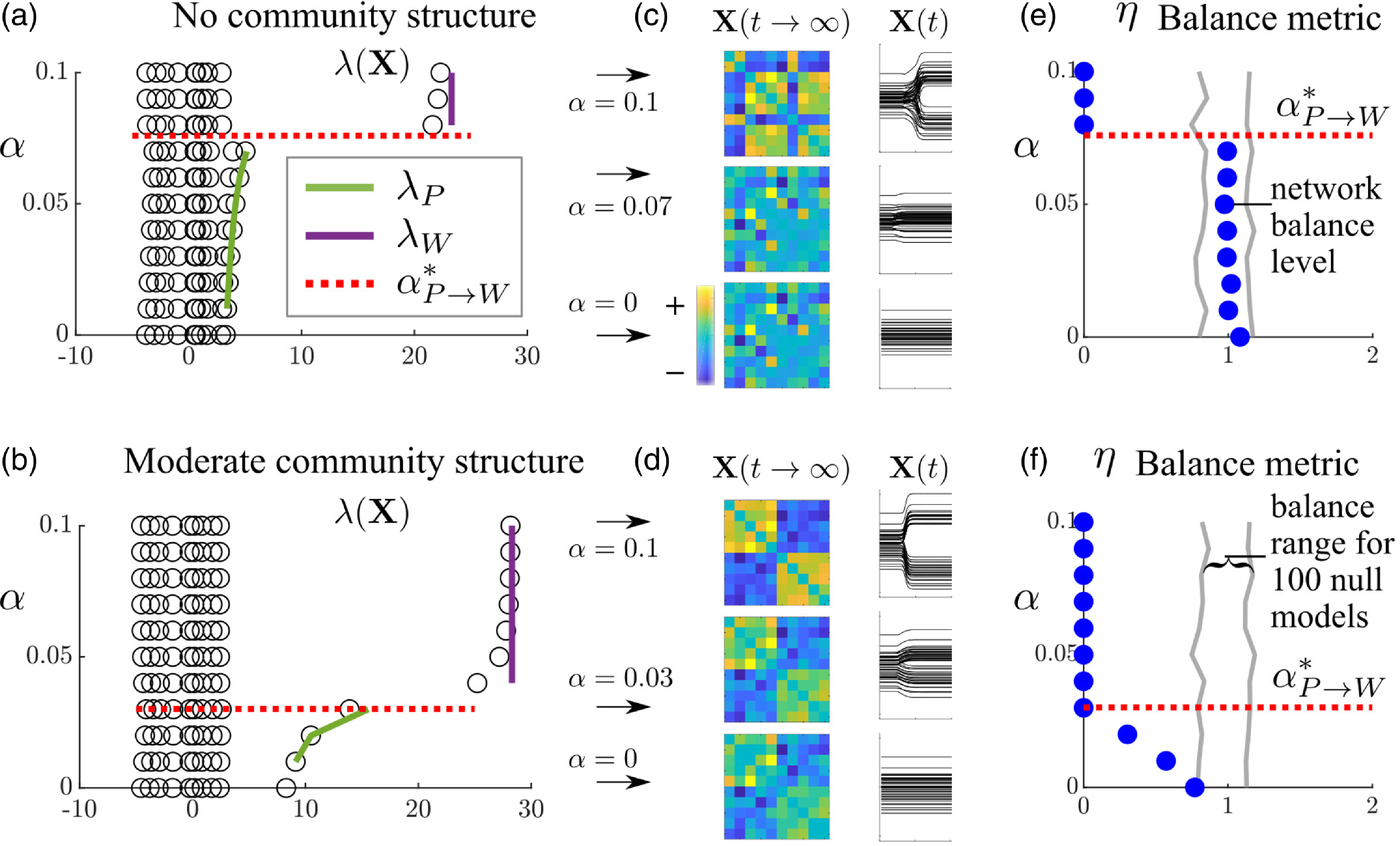
Figure 2. Effect of increasing structural balance sensitivity, $\alpha$
on eigenvalues,
$\alpha$
on eigenvalues, $\lambda _i$
, and balance levels,
$\lambda _i$
, and balance levels, $\eta$
, of the dynamic network at equilibrium.
$\eta$
, of the dynamic network at equilibrium. $L=2$
,
$L=2$
, $\beta =1$
, and
$\beta =1$
, and $N=10$
. (a) Stable state eigenvalues as a function of
$N=10$
. (a) Stable state eigenvalues as a function of $\alpha$
resulting from a random bias network containing no community structure,
$\alpha$
resulting from a random bias network containing no community structure, $\textbf{X}_{Dij} \sim 0.8 \mathcal{N}\,(0,1)$
. Theoretically computed bifurcation value
$\textbf{X}_{Dij} \sim 0.8 \mathcal{N}\,(0,1)$
. Theoretically computed bifurcation value $\alpha _{P \rightarrow W}^*$
(Equation (6)),
$\alpha _{P \rightarrow W}^*$
(Equation (6)), $\lambda _P$
(Equation (17)), and
$\lambda _P$
(Equation (17)), and $\lambda _W$
(Equation (19)). (b) Stable state eigenvalues resulting from a bias network with polarized community structure,
$\lambda _W$
(Equation (19)). (b) Stable state eigenvalues resulting from a bias network with polarized community structure, $X_{Dij} \sim 0.8 \mathcal{N}\,(0,1) +0.8 N u_{Ci}u_{Cj}$
. (c) Equilibrium dynamic networks and tie time series for
$X_{Dij} \sim 0.8 \mathcal{N}\,(0,1) +0.8 N u_{Ci}u_{Cj}$
. (c) Equilibrium dynamic networks and tie time series for $\alpha = 0.1$
,
$\alpha = 0.1$
, $\alpha = 0.07$
, and
$\alpha = 0.07$
, and $\alpha = 0$
for
$\alpha = 0$
for $\textbf{X}_D$
without community structure. (diagonals set to zero) (d) Equilibrium dynamic networks and tie time series for
$\textbf{X}_D$
without community structure. (diagonals set to zero) (d) Equilibrium dynamic networks and tie time series for $\alpha =0.1$
,
$\alpha =0.1$
, $\alpha =0.03$
, and
$\alpha =0.03$
, and $\alpha =0$
for
$\alpha =0$
for $\textbf{X}_D$
with community structure. (e) Balance levels
$\textbf{X}_D$
with community structure. (e) Balance levels $\eta$
of the equilibrium network (blue circles) as a function of
$\eta$
of the equilibrium network (blue circles) as a function of $\alpha$
for the no initial community structure case. Lower and upper range of
$\alpha$
for the no initial community structure case. Lower and upper range of $\eta$
values from null model simulations shown as gray lines. (f) Equilibrium network balance levels for the initial community structure case. The green curves in (a) and (b) show the analytical expression, (17), for the first eigenvalue in the peace state.
$\eta$
values from null model simulations shown as gray lines. (f) Equilibrium network balance levels for the initial community structure case. The green curves in (a) and (b) show the analytical expression, (17), for the first eigenvalue in the peace state.
The spectrum of the case where $\textbf{X}_D$
contains polarized community structure is shown in Figure 2(b). For
$\textbf{X}_D$
contains polarized community structure is shown in Figure 2(b). For $\alpha =0$
, there is no structural balance force and the tie values remain at their dyadic biases as seen in the time series of Figure 2(d), so the equilibrium
$\alpha =0$
, there is no structural balance force and the tie values remain at their dyadic biases as seen in the time series of Figure 2(d), so the equilibrium $\textbf{X}$
spectrum is the same as
$\textbf{X}$
spectrum is the same as $\textbf{X}_D$
. Unlike the no structure case, the first eigenvalue is substantially larger than the rest reflecting the underlying two-block structure of
$\textbf{X}_D$
. Unlike the no structure case, the first eigenvalue is substantially larger than the rest reflecting the underlying two-block structure of $\textbf{X}_D$
, which can be seen in the
$\textbf{X}_D$
, which can be seen in the $\alpha =0$
matrix visualization. This community structure results in a much smaller
$\alpha =0$
matrix visualization. This community structure results in a much smaller $\alpha ^*_{P \rightarrow W}$
than the no structure case. This suggests that bias networks exhibiting clear polarized structure, strong enough to appear in the first eigenvalue, may be more easily destabilized than those without. We present a more general argument about this behavior in Section 6.
$\alpha ^*_{P \rightarrow W}$
than the no structure case. This suggests that bias networks exhibiting clear polarized structure, strong enough to appear in the first eigenvalue, may be more easily destabilized than those without. We present a more general argument about this behavior in Section 6.
Structurally balanced networks are comprised of balanced triads—those containing either one or three positive ties. Balance levels in signed networks can be measured by counting the number of balanced versus imbalanced triads that exist in the network. Kirkley et al. (Reference Kirkley, Cantwell and Newman2019) develop a global balance metric $\eta$
, where
$\eta$
, where $\eta = 0$
corresponds to perfect balance and
$\eta = 0$
corresponds to perfect balance and $\eta = 1$
corresponds to the average level of balance generated in null model simulations where the null models are generated by randomly swapping the signs of the ties in the observed network. Figure 2(e–f) shows the balance level of the network at its final equilibrium state relative to the range of balance levels observed in the null model instances, shown by the gray bands. When the blue dot moves outside of the gray band this indicates that the system is significantly more balanced than expected polarized the null process. The no initial community structure case does not show a significant level of balance until after the bifurcation (Figure 2(e)) at which point the dynamic network transitions to the war state and becomes perfectly balanced. The case where the bias network has initial community structure, in contrast, shows significant levels of balance, which smoothly increases with
$\eta = 1$
corresponds to the average level of balance generated in null model simulations where the null models are generated by randomly swapping the signs of the ties in the observed network. Figure 2(e–f) shows the balance level of the network at its final equilibrium state relative to the range of balance levels observed in the null model instances, shown by the gray bands. When the blue dot moves outside of the gray band this indicates that the system is significantly more balanced than expected polarized the null process. The no initial community structure case does not show a significant level of balance until after the bifurcation (Figure 2(e)) at which point the dynamic network transitions to the war state and becomes perfectly balanced. The case where the bias network has initial community structure, in contrast, shows significant levels of balance, which smoothly increases with $\alpha$
even before the bifurcation (Figure 2(f)). These plots show that the onset of war greatly increases the level of structural balance in the dynamic network. Yet, the community structure plot also reveals that it is possible for the dynamic network to be balanced in a statistical sense in the peace state. The fact that structural balance tends to characterize peace and increases due to major war has been observed empirically for the international system as noted above (See Section 2).
$\alpha$
even before the bifurcation (Figure 2(f)). These plots show that the onset of war greatly increases the level of structural balance in the dynamic network. Yet, the community structure plot also reveals that it is possible for the dynamic network to be balanced in a statistical sense in the peace state. The fact that structural balance tends to characterize peace and increases due to major war has been observed empirically for the international system as noted above (See Section 2).
The peace-to-war bifurcation threshold is given by
 \begin{align} \alpha ^*_{P\rightarrow W} = \frac{\beta }{4 \lambda _{D1}}, \end{align}
where $\lambda _{D1}$
is the leading eigenvalue of
$\lambda _{D1}$
is the leading eigenvalue of $\textbf{X}_D$
. We derive this expression in Appendix A. The values for
$\textbf{X}_D$
. We derive this expression in Appendix A. The values for $\alpha ^*_{P\rightarrow W}$
predicted by this formula are in good agreement with the observed thresholds as shown by the red dashed lines in Figure 2(a) and (b). The community structure case has a higher
$\alpha ^*_{P\rightarrow W}$
predicted by this formula are in good agreement with the observed thresholds as shown by the red dashed lines in Figure 2(a) and (b). The community structure case has a higher $\lambda _{D1}$
than the no structure case as seen in the
$\lambda _{D1}$
than the no structure case as seen in the $\alpha =0$
spectra, which by (6) lowers the bifurcation threshold.
$\alpha =0$
spectra, which by (6) lowers the bifurcation threshold.
Even without the derivation, Equation (6) can be motivated intuitively. That increasing the direct dyadic force strength $\beta$
increases
$\beta$
increases $\alpha ^*_{P\rightarrow W}$
makes sense as the dyadic force seeks to maintain the peace state of low conflict and cooperation. When the elements of
$\alpha ^*_{P\rightarrow W}$
makes sense as the dyadic force seeks to maintain the peace state of low conflict and cooperation. When the elements of $\textbf{X}_D$
are drawn from a zero mean distribution as in Figure 2, the squared eigenvalue,
$\textbf{X}_D$
are drawn from a zero mean distribution as in Figure 2, the squared eigenvalue, $\lambda _{D_i}^2$
, is proportional to the variance of
$\lambda _{D_i}^2$
, is proportional to the variance of $\textbf{X}_D$
carried by each eigenvector.Footnote
5
The appearance of
$\textbf{X}_D$
carried by each eigenvector.Footnote
5
The appearance of $\lambda _{D1}$
in the denominator of (6) then reflects the fact that networks with greater values of
$\lambda _{D1}$
in the denominator of (6) then reflects the fact that networks with greater values of $\lambda _{D1}$
are more polarized in the peace state and so more unstable to war.
$\lambda _{D1}$
are more polarized in the peace state and so more unstable to war.
We note that for sufficient net positivity in $\textbf{X}_D$
, a bifurcation between the peace state and the harmony state of universal high cooperation occurs as the balance sensitivity
$\textbf{X}_D$
, a bifurcation between the peace state and the harmony state of universal high cooperation occurs as the balance sensitivity $\alpha$
is increased, analogous to the peace-to-war transition. It is also possible to have a direct transition between the war and harmony states. In the pure structural balance dynamics model, Equation (1), the war-to-harmony transition occurs when strong two-faction community structure becomes subordinate to harmonious one-faction structure in the initial network (Morrison & Gabbay, Reference Morrison and Gabbay2020). We consequently expect our model (3) to likewise undergo this bifurcation for sufficiently strong structural balance and bias network structure. To illustrate this bifurcation, instead of varying
$\alpha$
is increased, analogous to the peace-to-war transition. It is also possible to have a direct transition between the war and harmony states. In the pure structural balance dynamics model, Equation (1), the war-to-harmony transition occurs when strong two-faction community structure becomes subordinate to harmonious one-faction structure in the initial network (Morrison & Gabbay, Reference Morrison and Gabbay2020). We consequently expect our model (3) to likewise undergo this bifurcation for sufficiently strong structural balance and bias network structure. To illustrate this bifurcation, instead of varying $\alpha$
, we will vary the dyadic bias parameters via the outgroup affinity
$\alpha$
, we will vary the dyadic bias parameters via the outgroup affinity $p_{\text{out}}^+$
, the (conditional) probability of forming a positive tie with the outgroup in the stochastic block model which can be used to generate
$p_{\text{out}}^+$
, the (conditional) probability of forming a positive tie with the outgroup in the stochastic block model which can be used to generate $\textbf{X}_D$
(see Section 6). In Figure 3(a-b), the reversal of dominant structure is observed in the crossing in the spectrum of
$\textbf{X}_D$
(see Section 6). In Figure 3(a-b), the reversal of dominant structure is observed in the crossing in the spectrum of $\textbf{X}_D$
and in the qualitative change in its leading eigenvector from polarized structure to a homogeneous structure. Recall that
$\textbf{X}_D$
and in the qualitative change in its leading eigenvector from polarized structure to a homogeneous structure. Recall that $\textbf{X}_D$
plays a double role as the initial value of the dynamic network and as persistent parameters in the dyadic bias force. For low
$\textbf{X}_D$
plays a double role as the initial value of the dynamic network and as persistent parameters in the dyadic bias force. For low $p_{\text{out}}^+$
values the leading eigenvector contains two factions while for large
$p_{\text{out}}^+$
values the leading eigenvector contains two factions while for large $p_{\text{out}}^+$
values the leading eigenvector contains homogeneous structure (Figure 3(b)). The spectrum of the final network, however, does not display a crossing (Figure 3(c)); nor is there a discontinuity in the first eigenvalue as in Figure 2. Instead, it is the components of the first eigenvector which manifest the discontinuous signature of the bifurcation (Figure 3(d)). The block structure of the first eigenvector components below
$p_{\text{out}}^+$
values the leading eigenvector contains homogeneous structure (Figure 3(b)). The spectrum of the final network, however, does not display a crossing (Figure 3(c)); nor is there a discontinuity in the first eigenvalue as in Figure 2. Instead, it is the components of the first eigenvector which manifest the discontinuous signature of the bifurcation (Figure 3(d)). The block structure of the first eigenvector components below $p_{\text{out}}^+=0.5$
yields the war state (Figure 3(b)), whereas the uniformly positive components above
$p_{\text{out}}^+=0.5$
yields the war state (Figure 3(b)), whereas the uniformly positive components above $p_{\text{out}}^+=0.5$
yields the harmony state.
$p_{\text{out}}^+=0.5$
yields the harmony state.
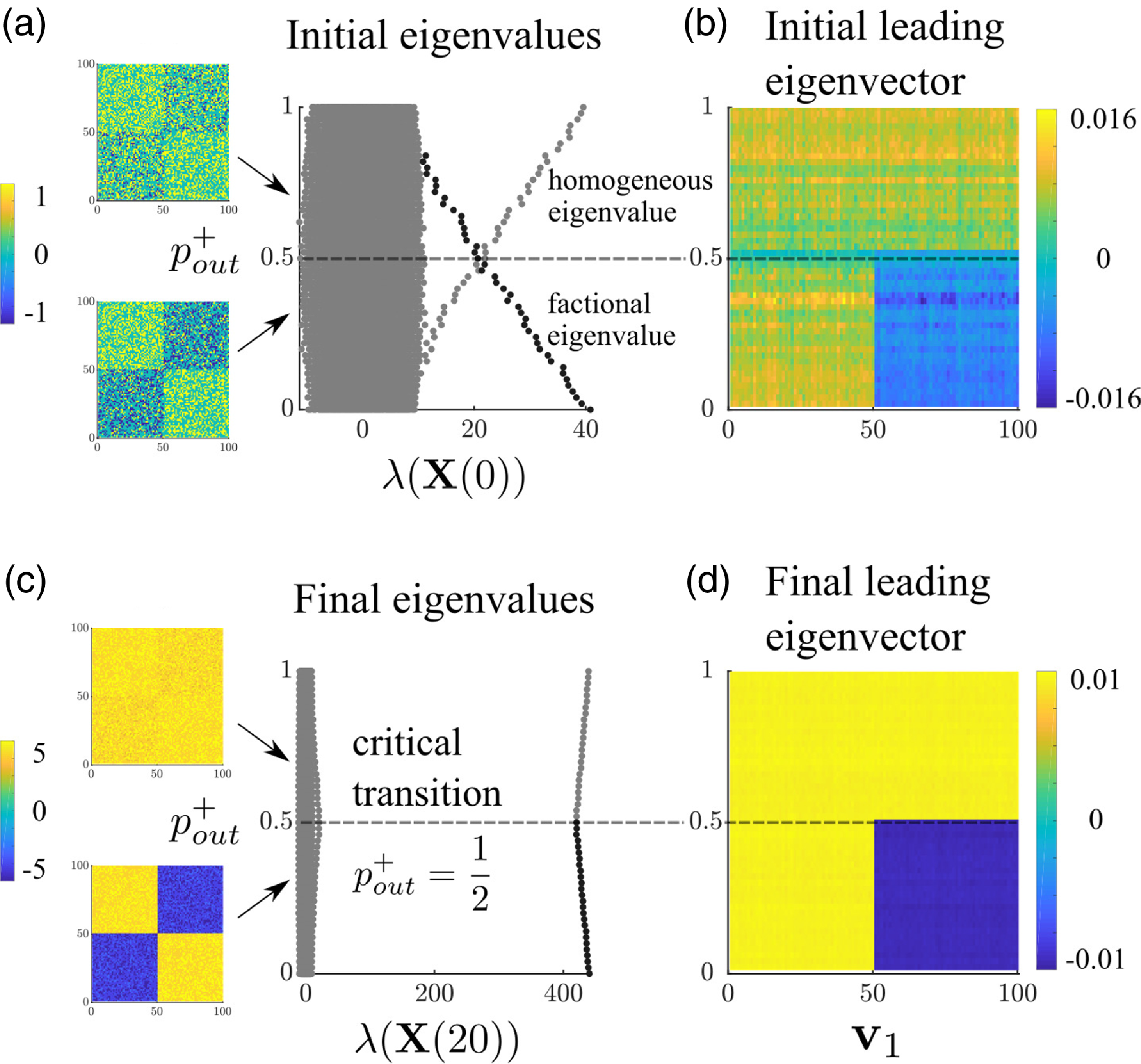
Figure 3. Simulation illustrating war-to-harmony bifurcation. (a) Eigenvalue spectrum of $\textbf{X}_D$
, also equivalent to initial dynamic network
$\textbf{X}_D$
, also equivalent to initial dynamic network $\textbf{X}(0)$
, for varying outgroup affinity
$\textbf{X}(0)$
, for varying outgroup affinity $p_{out}^+$
. Sample matrices at left depict how the ties are more positive and community structure is weaker above the crossing at
$p_{out}^+$
. Sample matrices at left depict how the ties are more positive and community structure is weaker above the crossing at $p_{out}^+=0.5$
than below. (b) Components of leading eigenvector of
$p_{out}^+=0.5$
than below. (b) Components of leading eigenvector of $\textbf{X}_D$
. When the leading eigenvector only has values
$\textbf{X}_D$
. When the leading eigenvector only has values $\geq 0$
, the corresponding leading eigenvalue is labeled as “homogeneous” while when the leading eigenvector has both positive and negative values, the corresponding eigenvalue is labeled as “factional”. (c) Eigenvalues of the equilibrium network after simulation of Equation (3) with
$\geq 0$
, the corresponding leading eigenvalue is labeled as “homogeneous” while when the leading eigenvector has both positive and negative values, the corresponding eigenvalue is labeled as “factional”. (c) Eigenvalues of the equilibrium network after simulation of Equation (3) with $N=100$
,
$N=100$
, $\beta = 1$
,
$\beta = 1$
, $\alpha = 0.02$
, and
$\alpha = 0.02$
, and $L=4$
. (d) Components of leading eigenvector of equilibrium network. Other stochastic block model parameters (see Section 6):
$L=4$
. (d) Components of leading eigenvector of equilibrium network. Other stochastic block model parameters (see Section 6): $d_{in}=d_{out} = 0.4$
,
$d_{in}=d_{out} = 0.4$
, $p_{in}^+=1$
.
$p_{in}^+=1$
.
5. Stability analysis
We now provide a mathematical explanation underlying the bifurcations seen in the simulations. First, we treat a simple special case that can be reduced to a one-dimensional system, yet illustrates the central aspects of the bifurcation behavior. We determine approximate formulas for the equilibria, both stable and unstable, in our dynamical system and use these to predict the critical value of the structural balance sensitivity at which the bifurcation occurs. We then summarize the results for the general case, which are derived in the Appendix.
5.1 Special case: Equal and opposite factions
Consider the special case where there are two equally sized, opposing factions in which all dyadic bias parameters have the same magnitude $\mu$
, but are positive for ties within the same faction and negative between factions so that
$\mu$
, but are positive for ties within the same faction and negative between factions so that $X_{Dij}=\pm \mu$
. We set the initial condition to be
$X_{Dij}=\pm \mu$
. We set the initial condition to be $X_{ij}(0)=X_{Dij}$
. Equation (3) then reduces to two equations,
$X_{ij}(0)=X_{Dij}$
. Equation (3) then reduces to two equations,
 \begin{align} \frac{dx}{dt} = -\beta (x-\mu )+L \tanh\!\left(\frac{\alpha N}{L}x^2\right) \end{align}
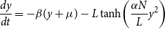 \begin{align} \frac{dy}{dt} = -\beta (y+\mu )-L \tanh\!\left(\frac{\alpha N}{L}y^2\right) \end{align}
for ingroup ties $x$
and outgroup ties
$x$
and outgroup ties $y$
, with initial conditions,
$y$
, with initial conditions, $x(0)=\mu$
and
$x(0)=\mu$
and $y(0)=-\mu$
. However, if we substitute
$y(0)=-\mu$
. However, if we substitute $y=-x$
in the bottom equation, we recover the top one and its initial condition, showing that the two equations are not independent. The system therefore reduces to one equation as solving for
$y=-x$
in the bottom equation, we recover the top one and its initial condition, showing that the two equations are not independent. The system therefore reduces to one equation as solving for $x$
using (7) then determines
$x$
using (7) then determines $y$
; the conflictual inter-faction ties are simply the negative of the cooperative intra-faction ties.
$y$
; the conflictual inter-faction ties are simply the negative of the cooperative intra-faction ties.
We make Equation (7) more tractable by replacing the hyperbolic tangent term on the positive axis with a piecewise linear approximation consisting of a line of unit slope connecting the origin to a plateau of height $L$
such that
$L$
such that $L^{\ast} \tanh(\theta/L) \rightarrow \theta$
for
$L^{\ast} \tanh(\theta/L) \rightarrow \theta$
for $0 \leq \theta \lt L$
and
$0 \leq \theta \lt L$
and $L^{\ast} \tanh(\theta/L) \rightarrow L$
for
$L^{\ast} \tanh(\theta/L) \rightarrow L$
for $\theta \geq L$
, where
$\theta \geq L$
, where $\theta =\alpha Nx^2$
. This approximation for the structural balance term is shown by the purple dashed line in Figure 4 (note it is piecewise linear in
$\theta =\alpha Nx^2$
. This approximation for the structural balance term is shown by the purple dashed line in Figure 4 (note it is piecewise linear in $\theta$
not
$\theta$
not $x$
, which is why the transition section is concave upwards). Under this approximation, Equation (7) becomes
$x$
, which is why the transition section is concave upwards). Under this approximation, Equation (7) becomes
 \begin{align} \frac{dx}{dt} = -\beta (x-\mu )+ \alpha Nx^2, \qquad 0 \leq x \lt \sqrt{\frac{L}{\alpha N}} \end{align}
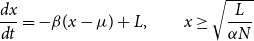 \begin{align} \frac{dx}{dt} = -\beta (x-\mu )+ L,\qquad x \geq \sqrt{\frac{L}{\alpha N}} \end{align}
Using these equations, we can derive simple formulas for the fixed points in the system: the peace and unstable fixed points will be obtained from (9) and the war fixed point from (10).

Figure 4. Strength of structural balance (purple) and direct dyadic (blue) forces and behavior of the equilibria in the special case. The approximations of the structural balance force (dashed) used in (9) and (10) agree well with the exact form (7) (solid), but are less accurate in the shoulder region. Stable (solid circles) and unstable (open circles) fixed points occur at intersections of balance and dyadic forces. $\alpha =0.03$
,
$\alpha =0.03$
, $L=6$
,
$L=6$
, $N=10$
, and
$N=10$
, and $\mu = 1/2$
.
$\mu = 1/2$
.
The equilibria of the above equations are found by setting $dx/dt=0$
, which implies that the direct dyadic and structural balance forces are of equal magnitude but of opposite sign. The right-hand side of Equation (9), being quadratic, has two roots. One yields the peace equilibrium,
$dx/dt=0$
, which implies that the direct dyadic and structural balance forces are of equal magnitude but of opposite sign. The right-hand side of Equation (9), being quadratic, has two roots. One yields the peace equilibrium, $x_p$
, which is stable and occurs at
$x_p$
, which is stable and occurs at
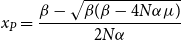 \begin{align} x_P = \frac{\beta - \sqrt{\beta (\beta - 4 N \alpha \mu )}}{2 N \alpha } \end{align}
The other fixed point is unstable and occurs at
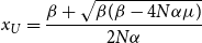 \begin{align} x_U = \frac{\beta + \sqrt{\beta (\beta - 4 N \alpha \mu )}}{2 N \alpha } \end{align}
Setting the right-hand side of Equation (10) to zero yields the fixed point corresponding to the war state, $x_w$
which is stable:
$x_w$
which is stable:
 \begin{align} x_W = \frac{L}{\beta } + \mu \end{align}
The above fixed points refer to the ingroup tie values—the outgroup tie values are their negatives. We observe that the structural balance force enters into these fixed points differently: for the war state via its maximum value, $L$
, whereas for the peace and unstable states via the sensitivity
$L$
, whereas for the peace and unstable states via the sensitivity $\alpha$
, which affects how much the structural balance force grows in response to changes around its neutral point. Equation (13) also explains our identification of the war tie value scale with
$\alpha$
, which affects how much the structural balance force grows in response to changes around its neutral point. Equation (13) also explains our identification of the war tie value scale with $L/\beta$
(see Section 3). Since the peace tie value scale is
$L/\beta$
(see Section 3). Since the peace tie value scale is $\mu$
, our assumption that the war tie values are much higher than the peace ones is equivalent to
$\mu$
, our assumption that the war tie values are much higher than the peace ones is equivalent to $L/\beta \gg \mu$
.
$L/\beta \gg \mu$
.
Figure 4 shows how the nature of the equilibrium solutions changes as the dyadic force strength parameter $\beta$
is varied while the structural balance parameters remain constant. The fixed points are located at the intersections of the linear dyadic force and the nonlinear structural balance force, where their magnitudes are equal but point in opposite directions with the dyadic force acting to decrease
$\beta$
is varied while the structural balance parameters remain constant. The fixed points are located at the intersections of the linear dyadic force and the nonlinear structural balance force, where their magnitudes are equal but point in opposite directions with the dyadic force acting to decrease $x$
(toward
$x$
(toward $\mu$
) and the balance force acting to increase
$\mu$
) and the balance force acting to increase $x$
. The stability of a fixed point with respect to small perturbations is determined by the relative magnitudes of the forces on either side of it. At moderate levels of the dyadic strength,
$x$
. The stability of a fixed point with respect to small perturbations is determined by the relative magnitudes of the forces on either side of it. At moderate levels of the dyadic strength, $\beta = 1$
, there are three fixed points in the system. The war equilibrium at
$\beta = 1$
, there are three fixed points in the system. The war equilibrium at $x_W\approx 6$
is stable since perturbations to its left (right) will be pulled back by the stronger balance (dyadic) force. The peace equilibrium at
$x_W\approx 6$
is stable since perturbations to its left (right) will be pulled back by the stronger balance (dyadic) force. The peace equilibrium at $x_P \approx 0.6$
is similarly stable. But the intermediate fixed point,
$x_P \approx 0.6$
is similarly stable. But the intermediate fixed point, $x_U$
is unstable since the stronger balance force pulls positive perturbations away from
$x_U$
is unstable since the stronger balance force pulls positive perturbations away from $x_U$
and towards
$x_U$
and towards $x_W$
and negative perturbations are drawn toward
$x_W$
and negative perturbations are drawn toward $x_P$
by the stronger dyadic force so that
$x_P$
by the stronger dyadic force so that $x \rightarrow x_W$
, when
$x \rightarrow x_W$
, when $x\gt x_U$
and
$x\gt x_U$
and $x \rightarrow x_P$
, when
$x \rightarrow x_P$
, when $x\lt x_U$
. When the dyadic strength is strong,
$x\lt x_U$
. When the dyadic strength is strong, $\beta = 2$
, the stable peace state in the only fixed point, so that
$\beta = 2$
, the stable peace state in the only fixed point, so that $x \rightarrow x_P$
for all
$x \rightarrow x_P$
for all $x$
. Finally, when the dyadic stability is weak,
$x$
. Finally, when the dyadic stability is weak, $\beta = 1/2$
, the stable war state at
$\beta = 1/2$
, the stable war state at $x_W \approx 12.5$
is the only fixed point so that
$x_W \approx 12.5$
is the only fixed point so that $x \rightarrow x_W$
for all
$x \rightarrow x_W$
for all $x$
(although it is difficult to discern in the figure, the dyadic and balance forces do not intersect at low
$x$
(although it is difficult to discern in the figure, the dyadic and balance forces do not intersect at low $x$
).
$x$
).
The bifurcation responsible for the changes between the different solution regimes is a saddle-node bifurcation. Two fixed points disappear when a stable fixed point collides with the unstable one as a parameter is changed. For example, if we increase $\beta$
starting from the
$\beta$
starting from the $\beta =1$
condition of Figure 4, the intersections determining
$\beta =1$
condition of Figure 4, the intersections determining $x_U$
and
$x_U$
and $x_W$
will draw closer together until they coincide when the dyadic force is tangent to the shoulder of the exact structural balance force (or intersects the corner of the approximate one). This coincidence point marks the war-to-peace bifurcation as it disappears upon further increase in
$x_W$
will draw closer together until they coincide when the dyadic force is tangent to the shoulder of the exact structural balance force (or intersects the corner of the approximate one). This coincidence point marks the war-to-peace bifurcation as it disappears upon further increase in $\beta$
, leaving only the
$\beta$
, leaving only the $x_P$
fixed point. Analogously, the peace-to-war bifurcation occurs when
$x_P$
fixed point. Analogously, the peace-to-war bifurcation occurs when $x_P$
and
$x_P$
and $x_U$
collide, leaving only
$x_U$
collide, leaving only $x_W$
.
$x_W$
.
We can now derive expressions relating to the parameters at the bifurcation points. The peace-to-war bifurcation occurs when $x_P = x_U$
. Equating (11) and (12) implies that the square root term must vanish, which yields the condition (ignoring the
$x_P = x_U$
. Equating (11) and (12) implies that the square root term must vanish, which yields the condition (ignoring the $\beta =0$
solution, which is simply pure structural balance),
$\beta =0$
solution, which is simply pure structural balance),
 \begin{align} \alpha ^*_{P\rightarrow W} = \frac{\beta }{4 N \mu } \end{align}
where we have solved for the critical value of the structural balance sensitivity. Similarly, the war-to-peace bifurcation occurs when $x_U=x_W$
. Equating (12) and (13) yields
$x_U=x_W$
. Equating (12) and (13) yields
 \begin{align} \alpha ^*_{W\rightarrow P} = \frac{L}{N(\mu +L/\beta )^2} \end{align}
Equation (14) shows that the peace-to-war transition occurs at larger $\alpha$
values for larger dyadic force strengths,
$\alpha$
values for larger dyadic force strengths, $\beta$
, a behavior that accords with the dyadic force’s role in stabilizing the peace equilibrium. Increasing the dyadic bias parameter,
$\beta$
, a behavior that accords with the dyadic force’s role in stabilizing the peace equilibrium. Increasing the dyadic bias parameter, $\mu$
, destabilizes the system at a lower
$\mu$
, destabilizes the system at a lower $\alpha ^*_{P\rightarrow W}$
, signifying that greater polarization in the peace state makes it more susceptible to war. Increasing the number of nodes
$\alpha ^*_{P\rightarrow W}$
, signifying that greater polarization in the peace state makes it more susceptible to war. Increasing the number of nodes $N$
also causes the peace state to become more fragile.Footnote
6
The dependence on
$N$
also causes the peace state to become more fragile.Footnote
6
The dependence on $L$
on the right-hand side of Equation (15) implies that the war-to-peace bifurcation sees the height of the balance force plateau, unlike the peace-to-war transition. Since
$L$
on the right-hand side of Equation (15) implies that the war-to-peace bifurcation sees the height of the balance force plateau, unlike the peace-to-war transition. Since $\alpha ^*_{W\rightarrow P}\rightarrow 0$
as
$\alpha ^*_{W\rightarrow P}\rightarrow 0$
as $L\rightarrow \infty$
, a larger
$L\rightarrow \infty$
, a larger $L$
, which corresponds to a larger level of cooperation and conflict in the war state, makes it more difficult for the system to transition back to the peace state.
$L$
, which corresponds to a larger level of cooperation and conflict in the war state, makes it more difficult for the system to transition back to the peace state.
5.2 General results
We consider bifurcations in the dynamics for the general case where the dyadic bias parameters can be different for each dyad. In addition, we allow for application of a transient perturbation which can induce a transition from the peace to the war state (or more generally a state of high tie values). We state the key results in this section and show the derivations leading to them in Appendix A.
Our dynamical system of edges, Equation (3), can be written succinctly as a matrix dynamical system
 \begin{align} \frac{d\textbf{X}}{dt} = -\beta (\textbf{X} - \textbf{X}_D) + L \tanh \!\left ( \frac{\alpha \textbf{X}^2}{L} \right ) + \textbf{X}_T(t) \end{align}
where $\textbf{X}$
is the symmetric matrix of ties
$\textbf{X}$
is the symmetric matrix of ties $X_{ij}$
,
$X_{ij}$
, $\textbf{X}_D$
is the matrix of the dyadic bias parameters,
$\textbf{X}_D$
is the matrix of the dyadic bias parameters, $X_{Dij}$
, and
$X_{Dij}$
, and $\textbf{X}_T(t)$
is the matrix of the transient perturbations
$\textbf{X}_T(t)$
is the matrix of the transient perturbations $X_{Tij}(t)$
. We can analyze the stability of the dynamics in the low-dimensional eigenvalue-eigenvector space of
$X_{Tij}(t)$
. We can analyze the stability of the dynamics in the low-dimensional eigenvalue-eigenvector space of $\textbf{X}$
and derive the system’s bifurcation conditions in terms of the leading eigenvalue of
$\textbf{X}$
and derive the system’s bifurcation conditions in terms of the leading eigenvalue of $\textbf{X}_D$
.
$\textbf{X}_D$
.
We first state the results in the absence of an imposed perturbation $\textbf{X}_T(t)$
. As in the special case, the peace-to-war transition is a saddle-node bifurcation. It occurs when the respective eigenvalues,
$\textbf{X}_T(t)$
. As in the special case, the peace-to-war transition is a saddle-node bifurcation. It occurs when the respective eigenvalues, $\lambda _P$
and
$\lambda _P$
and $\lambda _U$
, of the peace and unstable equilibria,
$\lambda _U$
, of the peace and unstable equilibria, $\textbf{X}_P$
and
$\textbf{X}_P$
and $\textbf{X}_U$
, merge. The general analysis approximates the structural balance term using
$\textbf{X}_U$
, merge. The general analysis approximates the structural balance term using $\tanh \theta \approx \theta$
for small
$\tanh \theta \approx \theta$
for small $\theta$
as in the special case. The leading eigenvalue of the peace state is given by
$\theta$
as in the special case. The leading eigenvalue of the peace state is given by
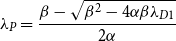 \begin{align} \lambda _P = \frac{\beta - \sqrt{\beta ^2 - 4\alpha \beta \lambda _{D1}}}{2 \alpha } \end{align}
where $\lambda _{D1}$
is the leading eigenvalue of the dyadic bias matrix
$\lambda _{D1}$
is the leading eigenvalue of the dyadic bias matrix $\textbf{X}_D$
. The lowest eigenvalue of the unstable state is the same as the expression for
$\textbf{X}_D$
. The lowest eigenvalue of the unstable state is the same as the expression for $\lambda _P$
, but with a positive sign in front of the square root term (see Equation (A18)). Setting
$\lambda _P$
, but with a positive sign in front of the square root term (see Equation (A18)). Setting $\lambda _P=\lambda _U$
, equivalent to the vanishing of the square root term above, yields the critical value for the structural balance sensitivity in the war-to-peace bifurcation,
$\lambda _P=\lambda _U$
, equivalent to the vanishing of the square root term above, yields the critical value for the structural balance sensitivity in the war-to-peace bifurcation,
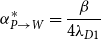 \begin{align} \alpha ^*_{P\rightarrow W} = \frac{\beta }{4 \lambda _{D1}} \end{align}
After the peace-to-war bifurcation, the system converges to the war equilibrium, $\textbf{X}_W$
, which has leading eigenvalue
$\textbf{X}_W$
, which has leading eigenvalue $\lambda _W$
. Using the flat plateau approximation of the structural balance force,
$\lambda _W$
. Using the flat plateau approximation of the structural balance force, $L \tanh \theta \approx \pm L$
for large
$L \tanh \theta \approx \pm L$
for large $|\theta |$
yields the following approximation for
$|\theta |$
yields the following approximation for $\lambda _W$
,
$\lambda _W$
,
 \begin{align} \lambda _W = \lambda _{D1} + \frac{L N}{\beta } \end{align}
The bifurcation from the war state back to the peace state occurs via a different saddle-node bifurcation where $\lambda _U = \lambda _W$
. The approximate condition for the war-to-peace bifurcation is then given by
$\lambda _U = \lambda _W$
. The approximate condition for the war-to-peace bifurcation is then given by
 \begin{align} \alpha ^*_{W\rightarrow P} &= \frac{NL}{(\lambda _{D1} + NL/\beta )^2} \end{align}
The general expressions for the critical $\alpha$
values, (18) and (20), are the same as in the special case except that
$\alpha$
values, (18) and (20), are the same as in the special case except that $N\mu$
has been replaced by
$N\mu$
has been replaced by $\lambda _{D1}$
(the next section shows that
$\lambda _{D1}$
(the next section shows that $\lambda _{D1} = N\mu$
in the special case). Figures 1 and 2 demonstrate how the analytically computed bifurcation values match the bifurcations observed through simulation. However, the peace-to-war estimated bifurcation is more accurate than the war-to-peace estimated bifurcation.
$\lambda _{D1} = N\mu$
in the special case). Figures 1 and 2 demonstrate how the analytically computed bifurcation values match the bifurcations observed through simulation. However, the peace-to-war estimated bifurcation is more accurate than the war-to-peace estimated bifurcation.
The analysis of the system with the transient perturbation term is restricted to the case when $\textbf{X}_T(t)$
is applied as an impulse in which all of its elements are constant for the duration of the impulse. In this case, the impact of
$\textbf{X}_T(t)$
is applied as an impulse in which all of its elements are constant for the duration of the impulse. In this case, the impact of $\textbf{X}_T(t)$
can be accounted for by a modified dyadic bias matrix,
$\textbf{X}_T(t)$
can be accounted for by a modified dyadic bias matrix, $\tilde{\textbf{X}}_D$
, that combines
$\tilde{\textbf{X}}_D$
, that combines $\textbf{X}_D$
and
$\textbf{X}_D$
and $\textbf{X}_T$
via
$\textbf{X}_T$
via
 \begin{align} \tilde{\textbf{X}}_D(t) = \textbf{X}_D + \frac{\textbf{X}_T(t)}{\beta } \end{align}
The threshold condition for $\textbf{X}_T(t)$
to induce the system to switch from the peace to the war state is analogous to the peace-to-war bifurcation in which
$\textbf{X}_T(t)$
to induce the system to switch from the peace to the war state is analogous to the peace-to-war bifurcation in which $\lambda _P=\lambda _U$
. However, the leading eigenvalue of the dyadic bias matrix in Equation (17) for
$\lambda _P=\lambda _U$
. However, the leading eigenvalue of the dyadic bias matrix in Equation (17) for $\lambda _P$
as well as that for
$\lambda _P$
as well as that for $\lambda _U$
(Equation (A18)) is replaced by the leading eigenvalue of
$\lambda _U$
(Equation (A18)) is replaced by the leading eigenvalue of $\tilde{\textbf{X}}_D$
, which we write as
$\tilde{\textbf{X}}_D$
, which we write as $\tilde{\lambda }_{D1}$
. Accordingly, the threshold condition is the same as the peace-to-war bifurcation condition, Equation (18), but with
$\tilde{\lambda }_{D1}$
. Accordingly, the threshold condition is the same as the peace-to-war bifurcation condition, Equation (18), but with $\tilde{\lambda }_{D1}$
instead of
$\tilde{\lambda }_{D1}$
instead of $\lambda _{D1}$
. For the imposed perturbation context, however, we keep the model parameters fixed and vary
$\lambda _{D1}$
. For the imposed perturbation context, however, we keep the model parameters fixed and vary $\textbf{X}_T$
, so it is more appropriate to cast the condition in terms of the critical value of
$\textbf{X}_T$
, so it is more appropriate to cast the condition in terms of the critical value of $\tilde{\lambda }_{D1}$
,
$\tilde{\lambda }_{D1}$
,
 \begin{align} \tilde{\lambda }_{D1}^* &= \frac{\beta }{4 \alpha } \end{align}
6. Enhancement of instability due to polarized community structure
We now use the results of the stability analysis above to generalize the behavior seen in the simulations in Figure 2 showing the greater instability of polarized community structure as compared with the no structure case, that is, its peace-to-war bifurcation occurs at a lower critical value $\alpha ^*_{P\rightarrow W}$
. We will show that systems whose bias networks have evident polarized structure have a lower
$\alpha ^*_{P\rightarrow W}$
. We will show that systems whose bias networks have evident polarized structure have a lower $\alpha ^*_{P\rightarrow W}$
than systems with bias networks for which such structure is not discernible. Discernible structure may be lacking because there is simply no tendency for preferential tie formation built into the stochastic process that generates the dyadic bias parameters
$\alpha ^*_{P\rightarrow W}$
than systems with bias networks for which such structure is not discernible. Discernible structure may be lacking because there is simply no tendency for preferential tie formation built into the stochastic process that generates the dyadic bias parameters $X_{Dij}$
(also taken as the initial conditions for the dynamic network); alternatively, the tendency is present but too weak to be discerned in the eigenvalue spectrum.
$X_{Dij}$
(also taken as the initial conditions for the dynamic network); alternatively, the tendency is present but too weak to be discerned in the eigenvalue spectrum.
We can create polarized community structure in $\textbf{X}_D$
with a signed network stochastic block model which assigns a positive, negative, or zero tie value between nodes with probabilities dependent on whether the nodes are drawn from the same block or different blocks (Morrison & Gabbay, Reference Morrison and Gabbay2020). The probability of a dyad being connected by any tie, whether positive or negative, is given by the ingroup tie density,
$\textbf{X}_D$
with a signed network stochastic block model which assigns a positive, negative, or zero tie value between nodes with probabilities dependent on whether the nodes are drawn from the same block or different blocks (Morrison & Gabbay, Reference Morrison and Gabbay2020). The probability of a dyad being connected by any tie, whether positive or negative, is given by the ingroup tie density, $d_{in}$
, for intra-block dyads and the outgroup tie density,
$d_{in}$
, for intra-block dyads and the outgroup tie density, $d_{out}$
, for inter-block dyads. The ingroup and outgroup affinities,
$d_{out}$
, for inter-block dyads. The ingroup and outgroup affinities, $p^+_{in}$
and
$p^+_{in}$
and $p^+_{out}$
, for the intra and inter-block dyads respectively are the probabilities of a positive tie conditional upon a tie being present. There are two blocks of equal size with the first comprising the first
$p^+_{out}$
, for the intra and inter-block dyads respectively are the probabilities of a positive tie conditional upon a tie being present. There are two blocks of equal size with the first comprising the first $N/2$
nodes,
$N/2$
nodes, $(1, \dots, N/2)$
and the other consisting of the next
$(1, \dots, N/2)$
and the other consisting of the next $N/2$
nodes,
$N/2$
nodes, $(N/2+1, \dots, N)$
. The generated bias network matrices can be written as the sum of an average “signal” matrix
$(N/2+1, \dots, N)$
. The generated bias network matrices can be written as the sum of an average “signal” matrix $\langle \textbf{X}_D \rangle$
and a zero mean random “noise” matrix. The signal matrix can be decomposed as the sum of two matrices formed by the outer products of its eigenvectors as follows:
$\langle \textbf{X}_D \rangle$
and a zero mean random “noise” matrix. The signal matrix can be decomposed as the sum of two matrices formed by the outer products of its eigenvectors as follows:
 \begin{align} \langle \textbf{X}_D \rangle &= N \omega \textbf{u}_H \textbf{u}_H^T + N \mu \textbf{u}_C \textbf{u}_C^T \end{align}
where $\textbf{u}_H = \frac{1}{\sqrt{N}}[1, 1, \ldots, 1]^T$
and
$\textbf{u}_H = \frac{1}{\sqrt{N}}[1, 1, \ldots, 1]^T$
and $\textbf{u}_C = \frac{1}{\sqrt{N}}[1,\ldots, 1, -1,\ldots, -1]^T$
are orthonormal vectors (the first negative component of
$\textbf{u}_C = \frac{1}{\sqrt{N}}[1,\ldots, 1, -1,\ldots, -1]^T$
are orthonormal vectors (the first negative component of $\textbf{u}_C$
is at
$\textbf{u}_C$
is at $N/2+1$
). The first term generates an
$N/2+1$
). The first term generates an $N \times N$
matrix all of whose elements are equal to
$N \times N$
matrix all of whose elements are equal to $\omega$
, the expected average of all the tie values in
$\omega$
, the expected average of all the tie values in $\langle \textbf{X}_D \rangle$
. The second term generates a matrix where the block diagonal ties are given by
$\langle \textbf{X}_D \rangle$
. The second term generates a matrix where the block diagonal ties are given by $+\mu$
and the off-diagonal blocks are
$+\mu$
and the off-diagonal blocks are $-\mu$
. We refer to
$-\mu$
. We refer to $\textbf{u}_H$
and
$\textbf{u}_H$
and $\textbf{u}_C$
as “signal eigenvectors.” As
$\textbf{u}_C$
as “signal eigenvectors.” As $\textbf{u}_H$
generates a uniform matrix, it is called the “homogeneous” eigenvector, whereas
$\textbf{u}_H$
generates a uniform matrix, it is called the “homogeneous” eigenvector, whereas $\textbf{u}_C$
is the “contrast” eigenvector as it generates the difference between intra-block and inter-block behavior. The noise matrix then accounts for the fact that, probabilistically, some ties will be absent or of opposite sign than expected for their block.
$\textbf{u}_C$
is the “contrast” eigenvector as it generates the difference between intra-block and inter-block behavior. The noise matrix then accounts for the fact that, probabilistically, some ties will be absent or of opposite sign than expected for their block.
The contrast parameter $\mu$
controls the level of polarization in the bias network. The block structure resulting from
$\mu$
controls the level of polarization in the bias network. The block structure resulting from $\mu \gt 0$
could reflect the operation of a homophily process, which results in preferential tie formation due for instance to similar ideology, religion, or ethnicity (the
$\mu \gt 0$
could reflect the operation of a homophily process, which results in preferential tie formation due for instance to similar ideology, religion, or ethnicity (the $\mu \lt 0$
case is not relevant here). The relative values of
$\mu \lt 0$
case is not relevant here). The relative values of $\omega$
and
$\omega$
and $\mu$
determine which kind of signal structure dominates: homogeneous if
$\mu$
determine which kind of signal structure dominates: homogeneous if $\omega \gt \mu$
and contrast if
$\omega \gt \mu$
and contrast if $\mu \gt \omega$
. The eigenvalues that go with
$\mu \gt \omega$
. The eigenvalues that go with $\textbf{u}_H$
and
$\textbf{u}_H$
and $\textbf{u}_C$
are given by, respectively,
$\textbf{u}_C$
are given by, respectively, $\lambda _H=N\omega$
and
$\lambda _H=N\omega$
and $\lambda _C=N\mu$
. Consequently, we can also use the relative values of
$\lambda _C=N\mu$
. Consequently, we can also use the relative values of $\lambda _H$
and
$\lambda _H$
and $\lambda _C$
to assess whether homogeneous or contrast structure dominates the signal. Note that the special case of equal and opposite factions above in which all intra-faction dyadic biases are
$\lambda _C$
to assess whether homogeneous or contrast structure dominates the signal. Note that the special case of equal and opposite factions above in which all intra-faction dyadic biases are $+\mu$
and all inter-faction ones are
$+\mu$
and all inter-faction ones are $-\mu$
can be completely constructed by the contrast eigenvector so that
$-\mu$
can be completely constructed by the contrast eigenvector so that $\textbf{X}_D = N \mu \textbf{u}_C \textbf{u}_C^T$
. The first (and only) eigenvalue of
$\textbf{X}_D = N \mu \textbf{u}_C \textbf{u}_C^T$
. The first (and only) eigenvalue of $\textbf{X}_D$
is then
$\textbf{X}_D$
is then $N\mu$
. This connects the special case result for the critical point
$N\mu$
. This connects the special case result for the critical point $\alpha ^*_{P\rightarrow W} = \beta/(4 N \mu )$
(Equation (14)) with the general result
$\alpha ^*_{P\rightarrow W} = \beta/(4 N \mu )$
(Equation (14)) with the general result $\alpha ^*_{P\rightarrow W} = \beta/(4 \lambda _{D1})$
(Equation (6)).
$\alpha ^*_{P\rightarrow W} = \beta/(4 \lambda _{D1})$
(Equation (6)).
If a signal eigenvalue is sufficiently large, then it will appear outside of the dense band of eigenvalues due to the noise. For example, in Figure 3(a), the contrast eigenvalue starts out as the leading eigenvalue at the bottom of the plot becomes the second eigenvalue after the signal crossing at $p^+_{out}=0.5$
, and then merges into the noise band around
$p^+_{out}=0.5$
, and then merges into the noise band around $p^+_{out}=0.8$
. This point corresponds to a phase transition for large
$p^+_{out}=0.8$
. This point corresponds to a phase transition for large $N$
, known as the community detectability transition (Nadakuditi & Newman, Reference Nadakuditi and Newman2012; Morrison & Gabbay, Reference Morrison and Gabbay2020). Past the detectability transition, even though the stochastic model still favors ingroup positive ties,
$N$
, known as the community detectability transition (Nadakuditi & Newman, Reference Nadakuditi and Newman2012; Morrison & Gabbay, Reference Morrison and Gabbay2020). Past the detectability transition, even though the stochastic model still favors ingroup positive ties, $p^+_{in}\gt p^+_{out}$
, this community structure cannot be identified given only the observed network.
$p^+_{in}\gt p^+_{out}$
, this community structure cannot be identified given only the observed network.
With this framework relating community structure to the bias network spectrum, we can address how polarized structure in the bias network affects the peace-to-war bifurcation threshold. The first eigenvector of $\textbf{X}_D$
contains polarized structure if it has components of opposite sign. That property alone, however, does not imply that the polarization is discernible—the first eigenvalue,
$\textbf{X}_D$
contains polarized structure if it has components of opposite sign. That property alone, however, does not imply that the polarization is discernible—the first eigenvalue, $\lambda _{D1}$
must also lie outside the positive edge of the noise band. This implies that
$\lambda _{D1}$
must also lie outside the positive edge of the noise band. This implies that $\lambda _{D1}$
is larger in the discernible polarization case than for the case when
$\lambda _{D1}$
is larger in the discernible polarization case than for the case when $\textbf{X}_D$
is generated from the noise only. Therefore, since Equation (6) states that
$\textbf{X}_D$
is generated from the noise only. Therefore, since Equation (6) states that $\alpha ^*_{P\rightarrow W}$
is inversely proportional to
$\alpha ^*_{P\rightarrow W}$
is inversely proportional to $\lambda _{D1}$
,
$\lambda _{D1}$
, $\alpha ^*_{P\rightarrow W}$
will be lower in the discernible polarization case as compared to the no polarization case. Consequently, the dynamical system in the discernible polarization case will be more prone to become unstable with respect to changes in system parameters that increase the balance sensitivity
$\alpha ^*_{P\rightarrow W}$
will be lower in the discernible polarization case as compared to the no polarization case. Consequently, the dynamical system in the discernible polarization case will be more prone to become unstable with respect to changes in system parameters that increase the balance sensitivity $\alpha$
. However, the operation of a homophily process presumed to generate polarization will not enhance instability if it is weak enough so that its spectral signature lies below the noise band.
$\alpha$
. However, the operation of a homophily process presumed to generate polarization will not enhance instability if it is weak enough so that its spectral signature lies below the noise band.
Although the above argument is based on two equal-sized blocks, stochastic block models with multiple, unequal blocks also display a spectral signature consisting of a noise band and outlying eigenvalues.Footnote
7
As long as the first bias network eigenvector contains community structure and its eigenvalue is discernible outside the noise band, then the system will be more sensitive to the peace-to-war bifurcation than when the structure is absent or submerged in the noise band. Therefore, instability will be enhanced whenever community structure is present in the first eigenvalue of $\textbf{X}_D$
, regardless of whether the blocks in the generating model are equal in size or how many blocks there are.
$\textbf{X}_D$
, regardless of whether the blocks in the generating model are equal in size or how many blocks there are.
Random matrix theory provides tools to analyze the noise matrix and so quantitatively assess the question of whether the first eigenvalue lies outside the band (Potters & Bouchaud, Reference Potters and Bouchaud2021). Expressions for the eigenvalue spectrum have been derived such as the Wigner semicircle law. In particular, the mean value of the band edge can be calculated as a function of the noise variance and the number of nodes, and the expected deviation of the band edge from the mean can be calculated as well. Consequently, the first eigenvalue can be taken as signal if it is sufficiently far outside the band edge expected from noise only.
7. Destabilizing directions of finite perturbations
Complex systems often exhibit nonlinear dynamics that have multiple stable states between which the system can transition (Strogatz & Dichter, Reference Strogatz and Dichter2016; Roberts, Reference Roberts2015). Random perturbations can induce transitions between states but it is also possible to investigate the effect of particular perturbations. Methods integrating bifurcation and control theories have been used to understand how targeted perturbations can be employed for control purposes in nonlinear dynamical networks, such as the hypothesized use of transient signals to shift between stable states in nematode locomotion or jumping between memory states in artificial neural networks (Morrison & Kutz, Reference Morrison and Kutz2021; Morrison et al., Reference Morrison and Kutz2021, Reference Morrison, Maia and Kutz2017). However, these methods can also be applied to the identification of deleterious perturbations, such as those that might trigger a major war. Identifying such perturbations may ultimately help in preventing them.
We now turn to the situation where our dynamical system, (16), can be shifted from one equilibrium to another, not by parameter changes, but by finite perturbations as contained in the matrix $\textbf{X}_T$
. Our goal here is to discover which patterns of dyads, if perturbed, are most dangerous in terms of destabilizing the peace state. We investigate this by determining what perturbations,
$\textbf{X}_T$
. Our goal here is to discover which patterns of dyads, if perturbed, are most dangerous in terms of destabilizing the peace state. We investigate this by determining what perturbations, $\textbf{X}_T$
, of a given size,
$\textbf{X}_T$
, of a given size, $||\textbf{X}_T||=c$
, move the system closest to the critical bifurcation threshold; these are the perturbation directions that are most dangerous as they are most likely to cause destabilization if they are too large. We measure how close the system is to a bifurcation by measuring how close the leading eigenvalue is to the critical bifurcation eigenvalue. First, we develop the mathematical framework for identifying these patterns according to different optimization conditions. We then illustrate how this framework can be applied using the network of five great power just before the onset of World War I.
$||\textbf{X}_T||=c$
, move the system closest to the critical bifurcation threshold; these are the perturbation directions that are most dangerous as they are most likely to cause destabilization if they are too large. We measure how close the system is to a bifurcation by measuring how close the leading eigenvalue is to the critical bifurcation eigenvalue. First, we develop the mathematical framework for identifying these patterns according to different optimization conditions. We then illustrate how this framework can be applied using the network of five great power just before the onset of World War I.
Destabilization of the peace state can be achieved through a change in model parameters as occurred in Figure 1(b) when the balance sensitivity was increased from 0.05 to 0.1; the peace equilibrium disappeared and the system shifted to the war state, the only equilibrium remaining. However, $\alpha =0.05$
resides in the bistable regime where both the peace and war equilibria are stable, as seen in Figure 1(c). Consequently, an alternative mode of destabilizing the peace state in the bistable regime is via a perturbation strong enough to kick the system into the war state. These perturbations may be localized to particular nodes, for example, a military crisis between two states. They are also assumed to be transient in duration so that, absent an escalation to system-wide war, the perturbed dyads will return to their equilibrium tie values.
$\alpha =0.05$
resides in the bistable regime where both the peace and war equilibria are stable, as seen in Figure 1(c). Consequently, an alternative mode of destabilizing the peace state in the bistable regime is via a perturbation strong enough to kick the system into the war state. These perturbations may be localized to particular nodes, for example, a military crisis between two states. They are also assumed to be transient in duration so that, absent an escalation to system-wide war, the perturbed dyads will return to their equilibrium tie values.
In our stability analysis results for the general case (Section 5.2), perturbations in $\textbf{X}_T$
were incorporated into a modified bias matrix,
$\textbf{X}_T$
were incorporated into a modified bias matrix, $\tilde{\textbf{X}}_D$
, with leading eigenvalue,
$\tilde{\textbf{X}}_D$
, with leading eigenvalue, $\tilde{\lambda }_{D1}$
. To shift from the peace to the war state in the bistable regime then requires that
$\tilde{\lambda }_{D1}$
. To shift from the peace to the war state in the bistable regime then requires that $\tilde{\lambda }_{D1}$
equal or exceed the eigenvalue of the unstable equilibrium,
$\tilde{\lambda }_{D1}$
equal or exceed the eigenvalue of the unstable equilibrium, $\lambda _{U}$
, with the critical eigenvalue denoted by
$\lambda _{U}$
, with the critical eigenvalue denoted by $\tilde{\lambda }^*_{D1}$
. The effect of the perturbation can therefore be seen as equivalent to a temporary change in the bias parameters of the system so that a saddle-node bifurcation is induced. This condition is given by Equation (22),
$\tilde{\lambda }^*_{D1}$
. The effect of the perturbation can therefore be seen as equivalent to a temporary change in the bias parameters of the system so that a saddle-node bifurcation is induced. This condition is given by Equation (22), $\tilde{\lambda }^*_{D1}=\beta/4\alpha$
, for the peace-to-war bifurcation. We analyze the types of perturbations,
$\tilde{\lambda }^*_{D1}=\beta/4\alpha$
, for the peace-to-war bifurcation. We analyze the types of perturbations, $\textbf{X}_T$
, that can most readily destabilize a system for a given
$\textbf{X}_T$
, that can most readily destabilize a system for a given $\textbf{X}_D$
. We first consider a special case for the perturbation matrix where
$\textbf{X}_D$
. We first consider a special case for the perturbation matrix where $\textbf{X}_T$
can be analytically calculated. We then present computational schemes to identify other destabilizing perturbations including those that may produce final states other than the war state that results from the peace-to-war bifurcation.
$\textbf{X}_T$
can be analytically calculated. We then present computational schemes to identify other destabilizing perturbations including those that may produce final states other than the war state that results from the peace-to-war bifurcation.
7.1 Minimum energy destabilization using dyadic bias leading eigenvector
The perturbation to the peace state that requires the least amount of energy, $||\textbf{X}_T||$
, to destabilize is along the direction of the leading eigenvector of
$||\textbf{X}_T||$
, to destabilize is along the direction of the leading eigenvector of $\textbf{X}_D$
, denoted by
$\textbf{X}_D$
, denoted by $\mathbf{s}_{D1}$
. The resulting perturbation matrix can be written as
$\mathbf{s}_{D1}$
. The resulting perturbation matrix can be written as $\textbf{X}_T =\sigma \mathbf{s}_{D1} \mathbf{s}_{D1}^T$
. We solve for the minimum value of
$\textbf{X}_T =\sigma \mathbf{s}_{D1} \mathbf{s}_{D1}^T$
. We solve for the minimum value of $\sigma$
that will destabilize the system (
$\sigma$
that will destabilize the system ( $||\textbf{X}_T||=\sigma$
). Destabilization requires that the leading eigenvalue of the modified dyadic bias matrix,
$||\textbf{X}_T||=\sigma$
). Destabilization requires that the leading eigenvalue of the modified dyadic bias matrix, $\tilde{\lambda }_{D1}$
, is at least as large as the critical eigenvalue so that
$\tilde{\lambda }_{D1}$
, is at least as large as the critical eigenvalue so that
 \begin{align} \tilde{\lambda }^*_{D1} & \leq \tilde{\lambda }_{D1} \end{align}
Making use of Equation (22) and the definition of $\tilde{\textbf{X}}_{D}$
, (21), then gives
$\tilde{\textbf{X}}_{D}$
, (21), then gives
 \begin{align} \frac{\beta }{4 \alpha } \leq \boldsymbol{\lambda _1} \!\left (\textbf{X}_D + \frac{\textbf{X}_T}{\beta } \right ) \end{align}
 \begin{align} \leq \boldsymbol{\lambda _1} \!\left (\textbf{X}_D + \frac{\sigma }{\beta } \mathbf{s}_{D1} \mathbf{s}_{D1}^T \right ) \end{align}
 \begin{align} \leq \lambda _{D1} + \frac{\sigma }{\beta } \end{align}
where the notation $\boldsymbol{\lambda _1}(\!\cdot\!)$
refers to the first eigenvalue of its argument and we have used
$\boldsymbol{\lambda _1}(\!\cdot\!)$
refers to the first eigenvalue of its argument and we have used $\textbf{X}_D \textbf{s}_{D1} = \lambda _{D1} \textbf{s}_{D1}$
and
$\textbf{X}_D \textbf{s}_{D1} = \lambda _{D1} \textbf{s}_{D1}$
and $\mathbf{s}_{D1}^T \mathbf{s}_{D1} = 1$
to show that
$\mathbf{s}_{D1}^T \mathbf{s}_{D1} = 1$
to show that $\textbf{s}_{D1}$
is also an eigenvector of
$\textbf{s}_{D1}$
is also an eigenvector of $\tilde{\textbf{X}}_D$
. Solving for
$\tilde{\textbf{X}}_D$
. Solving for $\sigma$
we find the condition required for destabilization,
$\sigma$
we find the condition required for destabilization,
 \begin{align} \sigma \geq \beta \!\left(\frac{\beta }{4 \alpha } - \lambda _{D1}\right) \end{align}
It is also useful to write this condition as
 \begin{align} \sigma \geq \beta (\tilde{\lambda }^*_{D1} - \lambda _{D1}) \end{align}
7.2 Destabilizing directions for perturbations
Although $\textbf{X}_T = \sigma \textbf{s}_{D1} \textbf{s}_{D1}^T$
is the perturbation that destabilizes the system with the minimum amount of energy (minimum
$\textbf{X}_T = \sigma \textbf{s}_{D1} \textbf{s}_{D1}^T$
is the perturbation that destabilizes the system with the minimum amount of energy (minimum $||\textbf{X}_T||$
), there are other, slightly higher energy perturbations that can also destabilize the system. We can search for perturbation directions within the space of perturbations
$||\textbf{X}_T||$
), there are other, slightly higher energy perturbations that can also destabilize the system. We can search for perturbation directions within the space of perturbations $||\textbf{X}_T||=\sigma$
that come closest to destabilizing the system. These are the perturbation directions that are most likely to destabilize the system since they require less energy to destabilize the system than other perturbations. We use the following optimization scheme to find perturbation directions
$||\textbf{X}_T||=\sigma$
that come closest to destabilizing the system. These are the perturbation directions that are most likely to destabilize the system since they require less energy to destabilize the system than other perturbations. We use the following optimization scheme to find perturbation directions $\textbf{X}_T$
that are closest to destabilizing the system for a given energy level
$\textbf{X}_T$
that are closest to destabilizing the system for a given energy level $||\textbf{X}_T|| = \sigma$
:
$||\textbf{X}_T|| = \sigma$
:
 \begin{align} \text{Energy minimizing scheme:} \quad \textbf{X}_T^{op}=&\mathop{\text{argmin}}_{\textbf{X}_T \in A}\left [ ||\tilde{\lambda }_{D1}^* - \tilde{\lambda }_{D1}|| \right ] \end{align}
where $A = \{\textbf{X}\;:\; ||\textbf{X}|| = \sigma \}$
,
$A = \{\textbf{X}\;:\; ||\textbf{X}|| = \sigma \}$
, $\tilde{\lambda }_{D1}$
is the leading eigenvalue of
$\tilde{\lambda }_{D1}$
is the leading eigenvalue of $\tilde{\textbf{X}}_D$
, and
$\tilde{\textbf{X}}_D$
, and $\tilde{\lambda }_{D1}^*$
is the stability threshold (Equation (22)). Energy minimizing perturbations result in minimal changes, on average, in tie strengths, whether positive or negative, since
$\tilde{\lambda }_{D1}^*$
is the stability threshold (Equation (22)). Energy minimizing perturbations result in minimal changes, on average, in tie strengths, whether positive or negative, since $||\textbf{X}_T||$
has been minimized. Equation (30) brings the system close to destabilization by perturbing the system in a direction close to the leading mode. We describe the destabilization scheme in more detail in Appendix B and Figure B1.
$||\textbf{X}_T||$
has been minimized. Equation (30) brings the system close to destabilization by perturbing the system in a direction close to the leading mode. We describe the destabilization scheme in more detail in Appendix B and Figure B1.
We now present two alternative destabilization schemes. The low-rank war state structure that appears after destabilizing the peace state will not necessarily contain two equally sized factions. The leading eigenvector could instead contain all nodes or mostly all nodes of the same sign. The interpretation of destabilization in this case would be instead the formation of a tightly-knit alliance structure where, due to structural balance dynamics, nodes are compelled to form positive ties with other nodes due to mutual allies. We can use the “eigenvector polarization” measure of the leading eigenvector, $\phi _1$
, to determine the extent to which the leading eigenvector contains community structure or a lack of community structure close to homogeneity (Morrison & Gabbay, in preparation). The eigenvector polarization
$\phi _1$
, to determine the extent to which the leading eigenvector contains community structure or a lack of community structure close to homogeneity (Morrison & Gabbay, in preparation). The eigenvector polarization $\phi _i$
of eigenvector
$\phi _i$
of eigenvector $\textbf{s}_i$
of the adjacency matrix
$\textbf{s}_i$
of the adjacency matrix $\textbf{X}$
is
$\textbf{X}$
is $\phi _i = \textbf{s}_i^T \textbf{M} \textbf{s}_i$
, where
$\phi _i = \textbf{s}_i^T \textbf{M} \textbf{s}_i$
, where $\textbf{M}$
is the signed modularity matrix (Traag et al., Reference Traag, Doreian and Mrvar2019; Newman, Reference Newman2006). The modularity matrix clusters nodes into communities.Footnote
8
If
$\textbf{M}$
is the signed modularity matrix (Traag et al., Reference Traag, Doreian and Mrvar2019; Newman, Reference Newman2006). The modularity matrix clusters nodes into communities.Footnote
8
If $\phi _1$
is the largest eigenvector polarization, then the network structure is dominated by polarization between two hostile factions.
$\phi _1$
is the largest eigenvector polarization, then the network structure is dominated by polarization between two hostile factions.
We use $\phi _1$
to define the following two schemes, which seek to: (1) bring the system close to destabilization with a widespread two-faction conflict (Equation (31)), or, alternatively, (2) bring the system close to destabilization with a widespread alliance bloc (Equation (32)).
$\phi _1$
to define the following two schemes, which seek to: (1) bring the system close to destabilization with a widespread two-faction conflict (Equation (31)), or, alternatively, (2) bring the system close to destabilization with a widespread alliance bloc (Equation (32)). $\textbf{X}_T^F$
indicates a perturbation that promotes factional structure in the leading eigenvector. A destabilizing perturbation that promotes factional structure will induce polarization in the system.
$\textbf{X}_T^F$
indicates a perturbation that promotes factional structure in the leading eigenvector. A destabilizing perturbation that promotes factional structure will induce polarization in the system. $\textbf{X}_T^H$
indicates a perturbation that promotes homogeneous structure in the leading eigenvector. A destabilizing perturbation that promotes homogeneous structure will induce harmony in the system.
$\textbf{X}_T^H$
indicates a perturbation that promotes homogeneous structure in the leading eigenvector. A destabilizing perturbation that promotes homogeneous structure will induce harmony in the system.
 \begin{align} \text{Polarizing:} \quad \textbf{X}_T^F=&\mathop{\text{argmin}}_{\textbf{X}_T \in A}\left [ ||\tilde{\lambda }_{D1}^* - \tilde{\lambda }_{D1}|| + \varepsilon \frac{1}{\phi _1} \right ] \end{align}
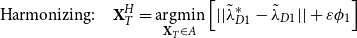 \begin{align} \text{Harmonizing:} \quad \textbf{X}_T^H=&\mathop{\text{argmin}}_{\textbf{X}_T \in A}\left [ ||\tilde{\lambda }_{D1}^* - \tilde{\lambda }_{D1}|| + \varepsilon \phi _1 \right ] \end{align}
Here, $\phi _1$
is the first eigenvector polarization measure of
$\phi _1$
is the first eigenvector polarization measure of $\tilde{\textbf{X}}_D$
, which changes as the perturbation
$\tilde{\textbf{X}}_D$
, which changes as the perturbation $\textbf{X}_T$
is varied, and
$\textbf{X}_T$
is varied, and $\varepsilon$
is its weighting. Forcing large changes in ties, whether increasing positive relations or increasing hostility requires more “energy” (a larger
$\varepsilon$
is its weighting. Forcing large changes in ties, whether increasing positive relations or increasing hostility requires more “energy” (a larger $||\textbf{X}_T||$
) than smaller perturbations in relations between countries. Because the leading eigenvector of the adjacency matrix may not contain factions, energy minimizing perturbations may not result in factions. The polarizing perturbation includes a faction-promoting term
$||\textbf{X}_T||$
) than smaller perturbations in relations between countries. Because the leading eigenvector of the adjacency matrix may not contain factions, energy minimizing perturbations may not result in factions. The polarizing perturbation includes a faction-promoting term $\frac{1}{\phi _1}$
, weighted by
$\frac{1}{\phi _1}$
, weighted by $\varepsilon$
, that is minimized when
$\varepsilon$
, that is minimized when $\phi _1$
is large. This promotes a solution where the leading eigenvector of the system contains factions. The extent to which factions are promoted is determined by the strength of
$\phi _1$
is large. This promotes a solution where the leading eigenvector of the system contains factions. The extent to which factions are promoted is determined by the strength of $\varepsilon$
(small enough values for
$\varepsilon$
(small enough values for $\varepsilon$
may not produce solutions that contain factions). The harmonizing perturbation, in contrast, deincentivizes factions in the leading eigenvector by including the faction-suppressing term
$\varepsilon$
may not produce solutions that contain factions). The harmonizing perturbation, in contrast, deincentivizes factions in the leading eigenvector by including the faction-suppressing term $\phi _1$
. The homogeneous perturbation is minimized when
$\phi _1$
. The homogeneous perturbation is minimized when $\phi _1$
is small which promotes a solution where the leading eigenvector of the system does not contain factions. These perturbation schemes assume that
$\phi _1$
is small which promotes a solution where the leading eigenvector of the system does not contain factions. These perturbation schemes assume that $\textbf{X}_T$
can be made large enough to result in a transition from the peace state to an equilibrium with high conflict and cooperation tie values (Figure B1(b)). If the maximum structural balance force strength,
$\textbf{X}_T$
can be made large enough to result in a transition from the peace state to an equilibrium with high conflict and cooperation tie values (Figure B1(b)). If the maximum structural balance force strength, $L$
, is sufficiently large, then the final state of the system will be determined by the first eigenvector of
$L$
, is sufficiently large, then the final state of the system will be determined by the first eigenvector of $\tilde{\textbf{X}}_D$
(see Equation (A24)). Therefore, as
$\tilde{\textbf{X}}_D$
(see Equation (A24)). Therefore, as $\textbf{X}_T$
can cause the leading eigenvector of
$\textbf{X}_T$
can cause the leading eigenvector of $\tilde{\textbf{X}}_D$
to be very different from that of
$\tilde{\textbf{X}}_D$
to be very different from that of $\textbf{X}_D$
, the high tie value state produced by the perturbation may contain very different factions than those in the war state arising from the peace-to-war bifurcation. While Equation (31) promotes factions in the systemic war equilibrium state and Equation (32) promotes a large alliance bloc encompassing most, if not all of the nodes, Equation (30) does not favor a particular structure in the war state, it simply emphasizes the structure most present in the dyadic bias matrix.
$\textbf{X}_D$
, the high tie value state produced by the perturbation may contain very different factions than those in the war state arising from the peace-to-war bifurcation. While Equation (31) promotes factions in the systemic war equilibrium state and Equation (32) promotes a large alliance bloc encompassing most, if not all of the nodes, Equation (30) does not favor a particular structure in the war state, it simply emphasizes the structure most present in the dyadic bias matrix.
8. Application to onset of World War I
8.1 World War I onset due to triggering perturbations
We use the maximally destabilizing directions formulas, Equations (30), (31), and (32), to find destabilizing directions for perturbations $\textbf{X}_T$
for the network of great powers leading up to the First World War under the dynamics of Equation (16). World War I is considered a classic example of a systemic war that emerged from the complex dynamics of five European great powers, the United Kingdom, France, Germany, Austria-Hungary, and Russia. We will compare our computationally derived destabilizing perturbation directions to ties that have been historically identified as critical to the outbreak of the Great War.
$\textbf{X}_T$
for the network of great powers leading up to the First World War under the dynamics of Equation (16). World War I is considered a classic example of a systemic war that emerged from the complex dynamics of five European great powers, the United Kingdom, France, Germany, Austria-Hungary, and Russia. We will compare our computationally derived destabilizing perturbation directions to ties that have been historically identified as critical to the outbreak of the Great War.
In order to illustrate our method on a simple system, we chose to only include the five most powerful European countries in the year 1913 in our network, as measured by the “Composite Index of National Capability” (CINC) score (Singer et al., Reference Singer, Bremer and Stuckey1972; Singer, Reference Singer1987). The scores range from $0.16$
(Germany) to
$0.16$
(Germany) to $0.06$
(Austria-Hungary). We exclude countries below this threshold as we do not weight the ties by country power and including the ties of less relevant countries adds “noise” to the relevant network structure. The next most powerful country below the cutoff is Italy with a score of
$0.06$
(Austria-Hungary). We exclude countries below this threshold as we do not weight the ties by country power and including the ties of less relevant countries adds “noise” to the relevant network structure. The next most powerful country below the cutoff is Italy with a score of $0.03$
, half that of Austria-Hungary. The political science literature also identifies these five countries as the most relevant to the outbreak of WWI (Kagan, Reference Kagan1995; Taylor, Reference Taylor1954). In other work we consider larger networks with many more countries (Morrison & Gabbay, in preparation); we are able to incorporate countries of vastly different sizes into the same network in this work by weighting each country’s ties by country power, resulting in a network that accurately reflects the relevance of each tie.
$0.03$
, half that of Austria-Hungary. The political science literature also identifies these five countries as the most relevant to the outbreak of WWI (Kagan, Reference Kagan1995; Taylor, Reference Taylor1954). In other work we consider larger networks with many more countries (Morrison & Gabbay, in preparation); we are able to incorporate countries of vastly different sizes into the same network in this work by weighting each country’s ties by country power, resulting in a network that accurately reflects the relevance of each tie.
We initialize the system using empirical data as follows. $\textbf{X}_D$
is set to the tie values in the year 1913 using the militarized interstate disputes (MIDs), alliances, and rivalries data from the Correlates of War dataset and the Handbook of International Rivalries (Palmer et al., Reference Palmer, D’Orazio, Kenwick and Lane2015; Gibler, Reference Gibler2009; Singer & Small, Reference Singer and Small1966; Thompson & Dreyer, Reference Thompson and Dreyer2011). Alliances contribute positive weights, MIDs contribute negative weights for states on opposite sides of a dispute and positive weights for states on the same side of a dispute, and rivalries contribute negative weights. Weights between states are added and scaled to range from −2 (rivals) to + 2 (allies), making all values in the dyadic bias matrix low-conflict/cooperation in comparison with the war levels of
$\textbf{X}_D$
is set to the tie values in the year 1913 using the militarized interstate disputes (MIDs), alliances, and rivalries data from the Correlates of War dataset and the Handbook of International Rivalries (Palmer et al., Reference Palmer, D’Orazio, Kenwick and Lane2015; Gibler, Reference Gibler2009; Singer & Small, Reference Singer and Small1966; Thompson & Dreyer, Reference Thompson and Dreyer2011). Alliances contribute positive weights, MIDs contribute negative weights for states on opposite sides of a dispute and positive weights for states on the same side of a dispute, and rivalries contribute negative weights. Weights between states are added and scaled to range from −2 (rivals) to + 2 (allies), making all values in the dyadic bias matrix low-conflict/cooperation in comparison with the war levels of $\pm 5$
as is roughly consistent with our assumption of peace and war having different tie scales.Footnote
9
(Table 2). Self-tie values are set to zero in the bias network. The dyadic force strength is set to
$\pm 5$
as is roughly consistent with our assumption of peace and war having different tie scales.Footnote
9
(Table 2). Self-tie values are set to zero in the bias network. The dyadic force strength is set to $\beta = 1$
, the balance sensitivity to
$\beta = 1$
, the balance sensitivity to $\alpha = 0.03$
, and
$\alpha = 0.03$
, and $L=5$
. With these parameter values the nonlinear dynamics contain two stable equilibrium, the peace state and war state, with the peace state sitting close to the unstable equilibrium. With initial conditions close to
$L=5$
. With these parameter values the nonlinear dynamics contain two stable equilibrium, the peace state and war state, with the peace state sitting close to the unstable equilibrium. With initial conditions close to $\textbf{X}_D$
, the network dynamics stabilize close to the bias network tie values. Since
$\textbf{X}_D$
, the network dynamics stabilize close to the bias network tie values. Since $\textbf{X}_D$
contains values in the range
$\textbf{X}_D$
contains values in the range $(\!-\!2,2)$
, the network stabilizes at the peace state when no perturbation is added to the system. The size of
$(\!-\!2,2)$
, the network stabilizes at the peace state when no perturbation is added to the system. The size of $\alpha$
does not affect the perturbation direction that is most destabilizing but instead the magnitude of perturbation necessary to surpass the destabilization threshold. We assume the system is sufficiently close to the peace-to-war bifurcation so that it resides in the bistable zone where both the war and peace equilibria are stable and that it can be destabilized with perturbations smaller than the dyadic bias matrix,
$\alpha$
does not affect the perturbation direction that is most destabilizing but instead the magnitude of perturbation necessary to surpass the destabilization threshold. We assume the system is sufficiently close to the peace-to-war bifurcation so that it resides in the bistable zone where both the war and peace equilibria are stable and that it can be destabilized with perturbations smaller than the dyadic bias matrix, $||\textbf{X}_T|| \lt ||\textbf{X}_D||$
. Setting
$||\textbf{X}_T|| \lt ||\textbf{X}_D||$
. Setting $\alpha = 0.03$
accomplishes these objectives. Making
$\alpha = 0.03$
accomplishes these objectives. Making $\alpha$
significantly larger would move the threshold past the necessity for a perturbation and the peace state would destabilize without the need for a perturbation. Setting
$\alpha$
significantly larger would move the threshold past the necessity for a perturbation and the peace state would destabilize without the need for a perturbation. Setting $\alpha$
significantly smaller would indicate that a destabilizing perturbation larger than the dyadic bias matrix would be required to destabilize the system and so perturbations would be unlikely to disrupt the status quo.
$\alpha$
significantly smaller would indicate that a destabilizing perturbation larger than the dyadic bias matrix would be required to destabilize the system and so perturbations would be unlikely to disrupt the status quo.
The left panel of Figure 5(a) shows the dyadic bias matrix, $\textbf{X}_D$
while the middle panel plots the eigenvalues of
$\textbf{X}_D$
while the middle panel plots the eigenvalues of $\textbf{X}_D$
, the eigenvalues of the modularity matrix
$\textbf{X}_D$
, the eigenvalues of the modularity matrix $\textbf{M}$
associated with
$\textbf{M}$
associated with $\textbf{X}_D$
, and the associated eigenvector polarization
$\textbf{X}_D$
, and the associated eigenvector polarization $\phi$
of all the eigenvectors. The leading eigenvalue of
$\phi$
of all the eigenvectors. The leading eigenvalue of $\textbf{X}_D$
has value
$\textbf{X}_D$
has value $\lambda _{D1}= 6.01$
, which is observed to be well separated from the remainder of the spectrum as is the first eigenvalue of the modularity matrix. The fact that
$\lambda _{D1}= 6.01$
, which is observed to be well separated from the remainder of the spectrum as is the first eigenvalue of the modularity matrix. The fact that $\phi _1$
is the largest eigenvector polarization signifies that
$\phi _1$
is the largest eigenvector polarization signifies that $\textbf{X}_D$
’s first eigenvector
$\textbf{X}_D$
’s first eigenvector $\textbf{s}_{D1}$
contains contrast-like community structure consisting of hostile factions (Morrison & Gabbay, in preparation). The two factions present in the leading eigenvector are the United Kingdom (UKG), France (FRN), and Russia (RUS) versus Germany (GMY) and Austria-Hungary (AUH). Also displayed is the critical eigenvalue of the modified dyadic bias matrix for destabilization, calculated from Equation (22) to be
$\textbf{s}_{D1}$
contains contrast-like community structure consisting of hostile factions (Morrison & Gabbay, in preparation). The two factions present in the leading eigenvector are the United Kingdom (UKG), France (FRN), and Russia (RUS) versus Germany (GMY) and Austria-Hungary (AUH). Also displayed is the critical eigenvalue of the modified dyadic bias matrix for destabilization, calculated from Equation (22) to be $\tilde{\lambda }_{D1}^* = 8.33$
. The optimum perturbation
$\tilde{\lambda }_{D1}^* = 8.33$
. The optimum perturbation $\textbf{X}_T^{op}$
that enables destabilization with the minimum energy is displayed in the right panel of Figure 5(a). It is proportional to the matrix formed by the first eigenvector of
$\textbf{X}_T^{op}$
that enables destabilization with the minimum energy is displayed in the right panel of Figure 5(a). It is proportional to the matrix formed by the first eigenvector of $\textbf{X}_D$
and is given by
$\textbf{X}_D$
and is given by $\textbf{X}_T^{op} =\sigma \mathbf{s}_{D1} \mathbf{s}_{D1}^T$
as explained in Section 7.1. The outer product of the leading eigenvector shows that FRN, GMY, AUH, and RUS are strongly entrenched in their respective factions while the outer product values for UKG are much closer to zero, indicating a looser affiliation with its faction. The minimum energy is calculated from Equation (29), which yields
$\textbf{X}_T^{op} =\sigma \mathbf{s}_{D1} \mathbf{s}_{D1}^T$
as explained in Section 7.1. The outer product of the leading eigenvector shows that FRN, GMY, AUH, and RUS are strongly entrenched in their respective factions while the outer product values for UKG are much closer to zero, indicating a looser affiliation with its faction. The minimum energy is calculated from Equation (29), which yields $\sigma = 2.32$
.
$\sigma = 2.32$
.
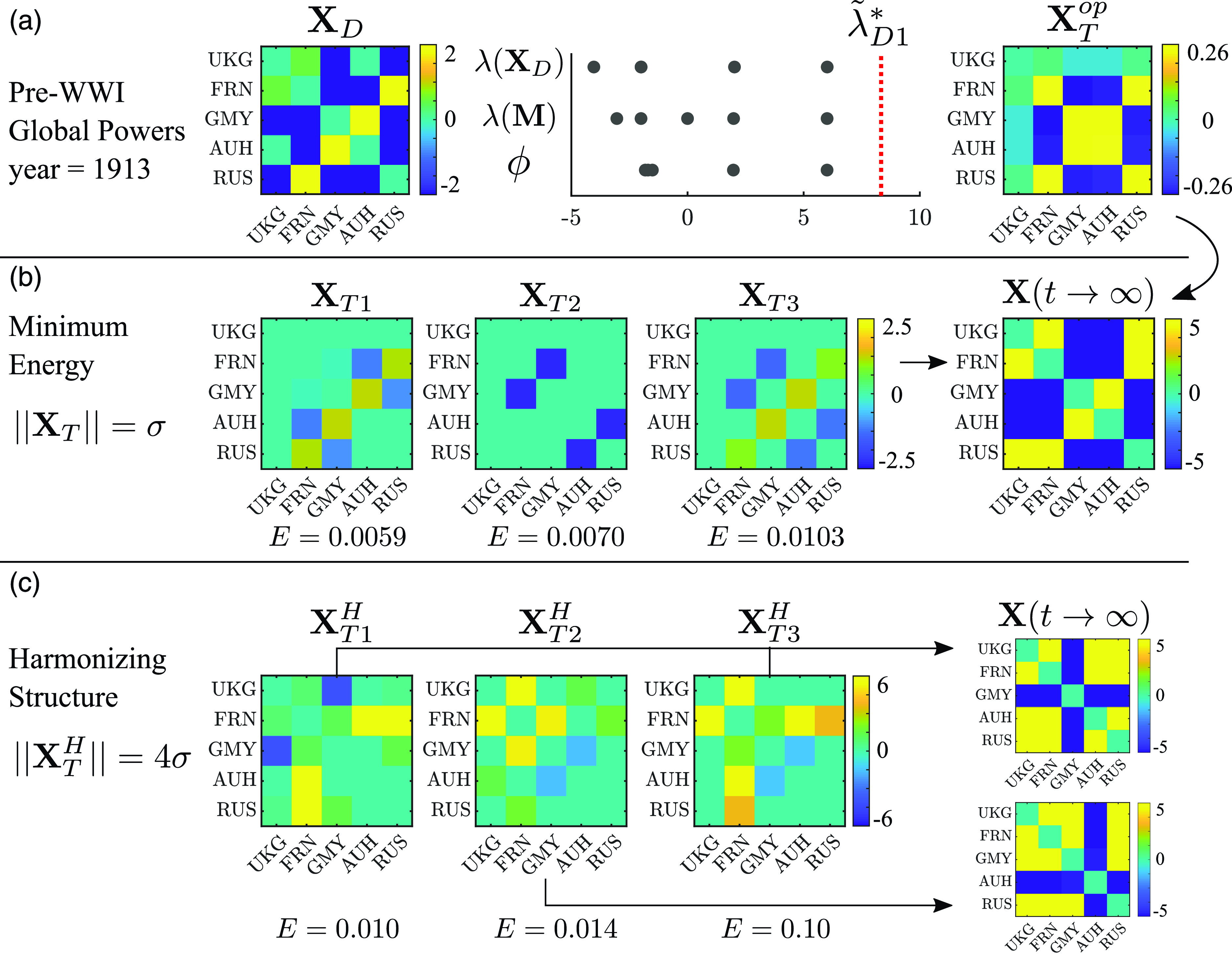
Figure 5. (a) $\textbf{X}_D$
is set to the tie weights of the great powers in 1913, immediately preceding WWI (left). Eigenvalue spectrum of
$\textbf{X}_D$
is set to the tie weights of the great powers in 1913, immediately preceding WWI (left). Eigenvalue spectrum of $\textbf{X}_D$
and modularity matrix, and eigenvector polarization spectrum (middle). Note that
$\textbf{X}_D$
and modularity matrix, and eigenvector polarization spectrum (middle). Note that $\phi_1$
is rightmost eigenvector polarization. For
$\phi_1$
is rightmost eigenvector polarization. For $\alpha = 0.03$
and
$\alpha = 0.03$
and $\beta =1$
, the bifurcation threshold is
$\beta =1$
, the bifurcation threshold is $\tilde{\lambda }_{D1}^* = 8.33$
. The leading eigenvalue of
$\tilde{\lambda }_{D1}^* = 8.33$
. The leading eigenvalue of $\textbf{X}_D$
is
$\textbf{X}_D$
is $\lambda _{D1}=6.01$
resulting in
$\lambda _{D1}=6.01$
resulting in $\sigma = 2.32$
. Minimum energy perturbation
$\sigma = 2.32$
. Minimum energy perturbation $\textbf{X}_T^{op}$
(right) leads to final state below. (b) Three perturbation directions requiring minimal energy (Equation (30)). Perturbations applied in these directions result in two factions in the leading eigenvector, and therefore two factions in the final state,
$\textbf{X}_T^{op}$
(right) leads to final state below. (b) Three perturbation directions requiring minimal energy (Equation (30)). Perturbations applied in these directions result in two factions in the leading eigenvector, and therefore two factions in the final state, $\textbf{X}(t \rightarrow \infty )$
. The factional structure perturbations (Equation (31)) are the same as the minimum energy perturbations for the WWI network. (c) Maximally destabilizing directions that have harmonizing structure (Equation (32)) result in a leading eigenvector with an almost homogeneous structure. Error minimized,
$\textbf{X}(t \rightarrow \infty )$
. The factional structure perturbations (Equation (31)) are the same as the minimum energy perturbations for the WWI network. (c) Maximally destabilizing directions that have harmonizing structure (Equation (32)) result in a leading eigenvector with an almost homogeneous structure. Error minimized, $E = \tilde{\lambda }_{D1}^* - \tilde{\lambda }_{D1}$
. Equation (A24) approximates equilibrium war states. Diagonal values in equilibrium states manually set to zero in network visualizations.
$E = \tilde{\lambda }_{D1}^* - \tilde{\lambda }_{D1}$
. Equation (A24) approximates equilibrium war states. Diagonal values in equilibrium states manually set to zero in network visualizations.
Substantively, the optimal perturbation matrix, $\textbf{X}_T^{op}$
, is marked by two tight factions—Germany and Austria-Hungary versus France and Russia; the United Kingdom is loosely aligned with the Franco-Russian bloc. This structure is consistent with the antagonisms and alliances that were most entwined in the several years before the war (Taylor, Reference Taylor1954; Kagan, Reference Kagan1995) Russia and Austria-Hungary competed for influence in the Balkans while France and Germany had severe territorial disputes and a history of animosity. France and Russia were allies as were Germany and Austria-Hungary. It is therefore reasonable that a crisis which activated tensions between the members of these alliances would be most efficient in triggering a war. In contrast, although the United Kingdom was aligned with France and Russia as a member of the Triple Entente, it was reluctant to get involved in Continental conflicts and its participation in the event of a war was uncertain.
$\textbf{X}_T^{op}$
, is marked by two tight factions—Germany and Austria-Hungary versus France and Russia; the United Kingdom is loosely aligned with the Franco-Russian bloc. This structure is consistent with the antagonisms and alliances that were most entwined in the several years before the war (Taylor, Reference Taylor1954; Kagan, Reference Kagan1995) Russia and Austria-Hungary competed for influence in the Balkans while France and Germany had severe territorial disputes and a history of animosity. France and Russia were allies as were Germany and Austria-Hungary. It is therefore reasonable that a crisis which activated tensions between the members of these alliances would be most efficient in triggering a war. In contrast, although the United Kingdom was aligned with France and Russia as a member of the Triple Entente, it was reluctant to get involved in Continental conflicts and its participation in the event of a war was uncertain.
The rightmost panel of Figure 5(b) shows the equilibrium state, $\textbf{X}(t\rightarrow \infty )$
, to which our dynamical model evolves the system as a result of a transient perturbation in the direction of
$\textbf{X}(t\rightarrow \infty )$
, to which our dynamical model evolves the system as a result of a transient perturbation in the direction of $\textbf{X}_T^{op}$
. The war state reached by the system matches the two opposing sides present during WWI with the United Kingdom, France, and Russia in one faction and Germany and Austria-Hungary in the other.
$\textbf{X}_T^{op}$
. The war state reached by the system matches the two opposing sides present during WWI with the United Kingdom, France, and Russia in one faction and Germany and Austria-Hungary in the other.
Going beyond the least energy perturbation, $\textbf{X}_T^{op}$
, we solve for alternative, sparse perturbation directions using the optimization functions delineated above, setting
$\textbf{X}_T^{op}$
, we solve for alternative, sparse perturbation directions using the optimization functions delineated above, setting $\sigma = 2.32$
, the energy level for the optimal solution. We compute the error as the amount to which the leading eigenvalue deviates from the stability threshold
$\sigma = 2.32$
, the energy level for the optimal solution. We compute the error as the amount to which the leading eigenvalue deviates from the stability threshold $E = \tilde{\lambda }_{D1}^* - \tilde{\lambda }_{D1}$
. The error tells us how close the system with a perturbation
$E = \tilde{\lambda }_{D1}^* - \tilde{\lambda }_{D1}$
. The error tells us how close the system with a perturbation $||\textbf{X}_T||=\sigma$
in the given direction is to destabilizing. Smaller values mean that the system is close to a bifurcation.
$||\textbf{X}_T||=\sigma$
in the given direction is to destabilizing. Smaller values mean that the system is close to a bifurcation.
Figure 5(b) shows three optimal sparse perturbation directions, $\textbf{X}_T$
, computed using Equation (30) from 100,000 randomly generated perturbations. These sparse perturbations have a substantial component in the direction of
$\textbf{X}_T$
, computed using Equation (30) from 100,000 randomly generated perturbations. These sparse perturbations have a substantial component in the direction of $\textbf{X}_T^{op}$
. All three involve only the Continental powers. The middle one,
$\textbf{X}_T^{op}$
. All three involve only the Continental powers. The middle one, $\textbf{X}_{T2}$
, depicts flare-ups in the two core rival dyads, France vs. Germany and Russia vs. Austria-Hungary. It was the assassination of Austrian Archduke Franz Ferdinand by a Serbian nationalist that set off a crisis between Austria-Hungary and Russia, Serbia’s ally, which ultimately led to the war. The right-hand perturbation,
$\textbf{X}_{T2}$
, depicts flare-ups in the two core rival dyads, France vs. Germany and Russia vs. Austria-Hungary. It was the assassination of Austrian Archduke Franz Ferdinand by a Serbian nationalist that set off a crisis between Austria-Hungary and Russia, Serbia’s ally, which ultimately led to the war. The right-hand perturbation, $\textbf{X}_{T3}$
, reflects increased cooperation between Germany and Austria-Hungary and between France and Russia as well as escalating tensions within the Austro-Hungarian–Russian and German–French rivalries. During the crisis, both Germany and France promised to come to the aid of their respective allies in the event of war whereas Britain, absent from this perturbation, was much more ambiguous about its intentions (Kissinger, Reference Kissinger1994). The lowest energy one,
$\textbf{X}_{T3}$
, reflects increased cooperation between Germany and Austria-Hungary and between France and Russia as well as escalating tensions within the Austro-Hungarian–Russian and German–French rivalries. During the crisis, both Germany and France promised to come to the aid of their respective allies in the event of war whereas Britain, absent from this perturbation, was much more ambiguous about its intentions (Kissinger, Reference Kissinger1994). The lowest energy one, $\textbf{X}_{T1}$
, represents an alternative scenario in which the conflicting dyads are France vs. Austria-Hungary and Russia vs. Germany with, again, support between allies. As with the optimal perturbation in Figure 5(a), all three perturbations when evolved by the dynamical model converge to the same two factions as present during WWI, as seen on the rightmost matrix of Figure 5(b).
$\textbf{X}_{T1}$
, represents an alternative scenario in which the conflicting dyads are France vs. Austria-Hungary and Russia vs. Germany with, again, support between allies. As with the optimal perturbation in Figure 5(a), all three perturbations when evolved by the dynamical model converge to the same two factions as present during WWI, as seen on the rightmost matrix of Figure 5(b).
We use Equation (31) to compute sparse perturbations that promote polarized structure and find the same perturbations as those found using the minimum energy scheme, and hence the polarizing scheme is not displayed as the results are identical to Figure 5(b). This occurs because the leading eigenvector of $\textbf{X}_D$
is already factional. These sparse perturbations have a substantial component in the direction of
$\textbf{X}_D$
is already factional. These sparse perturbations have a substantial component in the direction of $\textbf{X}_T^{op}$
. If the leading eigenvector of
$\textbf{X}_T^{op}$
. If the leading eigenvector of $\textbf{X}_D$
does not contain factional structure, then the perturbations obtained via Equation (31) will differ from the perturbations obtained via Equation (30). However, since the leading eigenvector of the WWI matrix does contain factional structure, Equations (31) and (30) return similar perturbations. As with the optimal perturbation, the perturbations in Figure 5(b) show that the United Kingdom’s ties with Continental Europe do not appear as significant in triggering conflict. This aligns with historical accounts that the United Kingdom was reluctant to get involved in Continental conflicts (Taylor, Reference Taylor1954; Kagan, Reference Kagan1995).
$\textbf{X}_D$
does not contain factional structure, then the perturbations obtained via Equation (31) will differ from the perturbations obtained via Equation (30). However, since the leading eigenvector of the WWI matrix does contain factional structure, Equations (31) and (30) return similar perturbations. As with the optimal perturbation, the perturbations in Figure 5(b) show that the United Kingdom’s ties with Continental Europe do not appear as significant in triggering conflict. This aligns with historical accounts that the United Kingdom was reluctant to get involved in Continental conflicts (Taylor, Reference Taylor1954; Kagan, Reference Kagan1995).
Figure 5(c) shows the harmonizing perturbations $\textbf{X}_T^H$
computed using Equation (32). The factional structure is much more dominant than other structures in
$\textbf{X}_T^H$
computed using Equation (32). The factional structure is much more dominant than other structures in $\textbf{X}_D$
resulting in a larger perturbation required to obtain a harmonious final state,
$\textbf{X}_D$
resulting in a larger perturbation required to obtain a harmonious final state, $||\textbf{X}_T^H|| = 4\sigma$
. Ideally, the harmonizing perturbations would result in a homogeneous structure among all nodes in the final equilibrium state. With a low level of perturbation energy, however, the system only manages to positively coalesce four of the five countries in a positive alliance bloc. Perturbations
$||\textbf{X}_T^H|| = 4\sigma$
. Ideally, the harmonizing perturbations would result in a homogeneous structure among all nodes in the final equilibrium state. With a low level of perturbation energy, however, the system only manages to positively coalesce four of the five countries in a positive alliance bloc. Perturbations $\textbf{X}_{P1}^H$
and
$\textbf{X}_{P1}^H$
and $\textbf{X}_{P3}^H$
lead to a homogeneous coalition against Germany while
$\textbf{X}_{P3}^H$
lead to a homogeneous coalition against Germany while $\textbf{X}_{P2}^H$
leads to a homogeneous coalition against Austria-Hungary.
$\textbf{X}_{P2}^H$
leads to a homogeneous coalition against Austria-Hungary.
Because the network, in this case, contains relatively few nodes ( $N=5$
), self-ties become a more relevant part of the dynamics. If self-ties are set to zero initially, the self-tie contribution to the force,
$N=5$
), self-ties become a more relevant part of the dynamics. If self-ties are set to zero initially, the self-tie contribution to the force, $\alpha (X_{ii} + X_{jj})X_{ij}$
, is also initially zero, yet grows in relevance as the self-ties grow, reinforcing the sign and strength of each tie. This adds to the escalation and makes it easier for the system to pass the destabilization threshold. We can also consider adding self-ties to the dyadic bias matrix, for example
$\alpha (X_{ii} + X_{jj})X_{ij}$
, is also initially zero, yet grows in relevance as the self-ties grow, reinforcing the sign and strength of each tie. This adds to the escalation and makes it easier for the system to pass the destabilization threshold. We can also consider adding self-ties to the dyadic bias matrix, for example $\textbf{X}_D \rightarrow \textbf{X}_D + c I$
, where
$\textbf{X}_D \rightarrow \textbf{X}_D + c I$
, where $c I$
is the identity matrix scaled by
$c I$
is the identity matrix scaled by $c$
. In this case the spectra of
$c$
. In this case the spectra of $\textbf{X}_D$
is shifted by
$\textbf{X}_D$
is shifted by $c$
, moving the system closer to the peace-to-war bifurcation. In both of these cases, self-ties contribute to system instability.
$c$
, moving the system closer to the peace-to-war bifurcation. In both of these cases, self-ties contribute to system instability.
8.2 World War I onset due to changes in dyadic bias community structure
We now take a different approach and evaluate which individual ties between two countries are most critical for increasing the leading eigenvalue and polarization of the dyadic bias matrix, $\textbf{X}_D$
, using tie values from the year 1913, preceding the outbreak of WWI. Given that increasing the first eigenvalue and polarization makes the system more susceptible to war, this analysis can identify which dyads most destabilize the system (or stabilize it if the first eigenvalue decreases). In Figure 6 we systematically shift the ties of
$\textbf{X}_D$
, using tie values from the year 1913, preceding the outbreak of WWI. Given that increasing the first eigenvalue and polarization makes the system more susceptible to war, this analysis can identify which dyads most destabilize the system (or stabilize it if the first eigenvalue decreases). In Figure 6 we systematically shift the ties of $\textbf{X}_D$
by
$\textbf{X}_D$
by $\varepsilon =\pm 1$
and observe the change each edge perturbation produces in the leading eigenvalue
$\varepsilon =\pm 1$
and observe the change each edge perturbation produces in the leading eigenvalue $\lambda _1$
and polarization
$\lambda _1$
and polarization $\phi _1$
, of
$\phi _1$
, of $\textbf{X}_D$
. Despite
$\textbf{X}_D$
. Despite $\textbf{X}_T$
consisting of only a single edge perturbation in each experiment, this small perturbation applied to
$\textbf{X}_T$
consisting of only a single edge perturbation in each experiment, this small perturbation applied to $\textbf{X}_D$
can result in large shifts in the leading eigenvalue and eigenvector polarization measure (Figure 6(a-b)). For example, Figure 6(b) illustrates how increasing hostilities between France and Austria,
$\textbf{X}_D$
can result in large shifts in the leading eigenvalue and eigenvector polarization measure (Figure 6(a-b)). For example, Figure 6(b) illustrates how increasing hostilities between France and Austria, $\varepsilon _{2,4} = -1$
, results in an increase in the leading eigenvalue. We represent each edge perturbation’s effect on
$\varepsilon _{2,4} = -1$
, results in an increase in the leading eigenvalue. We represent each edge perturbation’s effect on $\lambda _1$
and
$\lambda _1$
and $\phi _1$
in a succinct matrix format in Figure 6(c-f).
$\phi _1$
in a succinct matrix format in Figure 6(c-f).
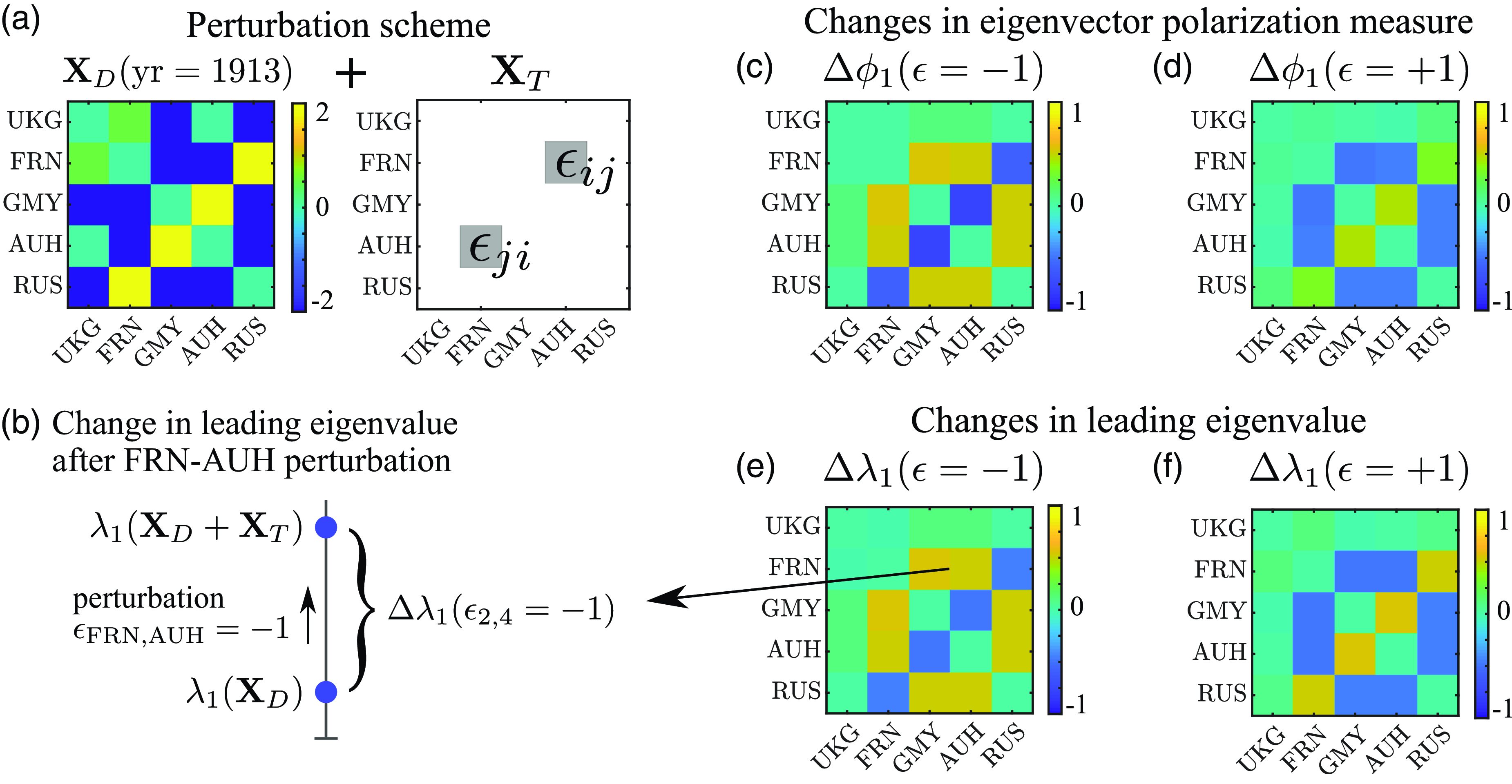
Figure 6. (a) Great powers network in 1913. (b) Increasing hostilities between France and Austria increases the leading eigenvalue of the network connectivity matrix. (c) Changes in $\phi _1$
for a
$\phi _1$
for a $\varepsilon = -1$
edge perturbation applied individually to each pair of nodes. Colors for each box in the matrix indicate the change in
$\varepsilon = -1$
edge perturbation applied individually to each pair of nodes. Colors for each box in the matrix indicate the change in $\phi _1$
when a perturbation is applied to that pair of nodes. (d) Changes in
$\phi _1$
when a perturbation is applied to that pair of nodes. (d) Changes in $\phi _1$
for
$\phi _1$
for $\varepsilon = +1$
perturbations. (e) Changes in
$\varepsilon = +1$
perturbations. (e) Changes in $\lambda _1$
for
$\lambda _1$
for $\varepsilon = -1$
perturbations. (f) Changes in
$\varepsilon = -1$
perturbations. (f) Changes in $\lambda _1$
for
$\lambda _1$
for $\varepsilon = +1$
perturbations. Self-ties were not considered.
$\varepsilon = +1$
perturbations. Self-ties were not considered.
Figure 6(c-f) shows that the tie between France and Germany as well as the tie between Germany and Austria-Hungary were the most crucial in increasing polarization in the network. The ties between Great Britain and the Continental countries appear to be the least important, implying that while Great Britain formed an important part of the network, changes in ties with this state least impact the stability of the system. Other significant ties include FRN-AUH, FRN-RUS, GMY-RUS, and AUH-RUS. This finding is to be expected as the German alliance with Austria-Hungary and their disputes with Russia as well as the alliance between Russia and France were all factors that proved integral to the development of World War I (Kagan, Reference Kagan1995; Taylor, Reference Taylor1954).
9. Critical slowing down near bifurcations
The destabilization analyses in the preceding section required knowledge of the dynamical system governing state dynamics and therefore the location of the bifurcation point could be calculated. However, a fully descriptive and predictive model governing the dynamics of real-world complex systems—physical, biological, and social—is often unknown in the sense that precise and accurate functional forms and parameter values are not available. This makes it difficult to empirically determine the distance in parameter space from a bifurcation. Yet, the fact that the behavior in the vicinity of a bifurcation is universal for all systems that undergo that type of bifurcation can help with this task. The theory of critical transitions seeks to develop early warning signals of impending bifurcations based on this universality (Kuehn, Reference Kuehn2011; Scheffer et al., 2012). One common signature is critical slowing down, in which the transients due to perturbations take longer to die down as the bifurcation is neared. Critical slowing down has been empirically observed in transitions in the climate, ecosystems, and neurons (Dakos et al., Reference Dakos, Scheffer, van Nes, Brovkin, Petoukhov and Held2008; Bury et al., Reference Bury, Sujith, Pavithran, Scheffer, Lenton, Anand and Bauch2021; Meisel et al., Reference Meisel, Klaus, Kuehn and Plenz2015).
Saddle-node bifurcations exhibit critical slowing down and so it should occur in our model dynamics and could be used to infer distance to the bifurcation in a real system in the absence of exact governing equations. Meisel et al. (Reference Meisel, Klaus, Kuehn and Plenz2015) found that for saddle-node bifurcations occurring in neural dynamics the recovery rate $r=\frac{1}{\tau }$
, where
$r=\frac{1}{\tau }$
, where $\tau$
is the decay time, scales with the square root of the distance from the bifurcation,
$\tau$
is the decay time, scales with the square root of the distance from the bifurcation, $r \propto \sqrt{d}$
, a scaling law that can be derived from the saddle-node normal form. Accordingly, we investigate whether our model follows this same scaling law.
$r \propto \sqrt{d}$
, a scaling law that can be derived from the saddle-node normal form. Accordingly, we investigate whether our model follows this same scaling law.
In Figure 7, we measure the leading eigenvalue of the system in the peaceful state while applying small perturbations to Equation (16). We then compute the recovery rate for these perturbations as $\alpha \rightarrow \alpha ^*$
. Perturbations are applied in the direction of the state at which the system has stabilized prior to the perturbation. When
$\alpha \rightarrow \alpha ^*$
. Perturbations are applied in the direction of the state at which the system has stabilized prior to the perturbation. When $\alpha$
is far from its bifurcation point and small perturbations are applied to the system the network activity decays quickly back to equilibrium (Figure 7(a)). When
$\alpha$
is far from its bifurcation point and small perturbations are applied to the system the network activity decays quickly back to equilibrium (Figure 7(a)). When $\alpha$
is close to its bifurcation point and small perturbations are applied to the system the network activity decays back to equilibrium much more slowly (Figure 7(b)). The system moves to the war state when small perturbations are applied to the system when
$\alpha$
is close to its bifurcation point and small perturbations are applied to the system the network activity decays back to equilibrium much more slowly (Figure 7(b)). The system moves to the war state when small perturbations are applied to the system when $\alpha = \alpha ^*$
(Figure 7(c)). Figure 7(d) shows that
$\alpha = \alpha ^*$
(Figure 7(c)). Figure 7(d) shows that $\log\!(r)$
scales linearly with
$\log\!(r)$
scales linearly with $\log\!(d)$
. A linear fit to the data finds that
$\log\!(d)$
. A linear fit to the data finds that $\log\!(r) = 0.49 \log\!(d)+1.23$
. This means that the recovery rate and distance to the bifurcation are related by
$\log\!(r) = 0.49 \log\!(d)+1.23$
. This means that the recovery rate and distance to the bifurcation are related by $r \approx 3.42 d^{\, 0.49}$
in good agreement with the square root scaling predicted for saddle-node bifurcations.
$r \approx 3.42 d^{\, 0.49}$
in good agreement with the square root scaling predicted for saddle-node bifurcations.
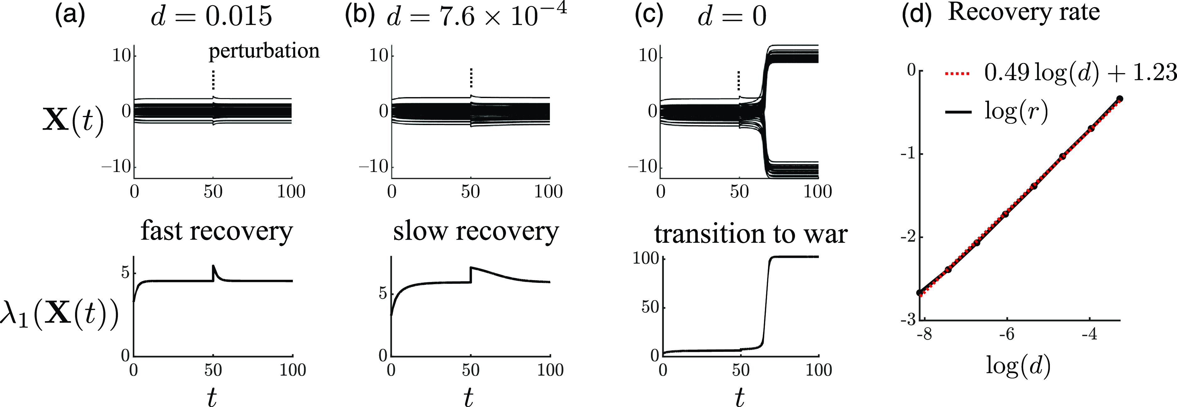
Figure 7. Critical slowing down near bifurcation. Recovery rate $r$
is a function of the distance
$r$
is a function of the distance $d$
to the bifurcation in the parameter
$d$
to the bifurcation in the parameter $\alpha$
,
$\alpha$
, $d = \alpha ^* - \alpha$
.
$d = \alpha ^* - \alpha$
. $N = 10$
,
$N = 10$
, $\beta = 1$
,
$\beta = 1$
, $L=10$
,
$L=10$
, $X_{ij}(0)=X_{Dij}$
,
$X_{ij}(0)=X_{Dij}$
, $X_{Dij} \sim 0.8 \mathcal{N}\,(0,1)$
. The perturbations,
$X_{Dij} \sim 0.8 \mathcal{N}\,(0,1)$
. The perturbations, $\textbf{X}_{T}(t)$
, used to measure recovery rate, are in the direction of the system’s stable state. (a) System perturbed when
$\textbf{X}_{T}(t)$
, used to measure recovery rate, are in the direction of the system’s stable state. (a) System perturbed when $\alpha$
is far from the bifurcation,
$\alpha$
is far from the bifurcation, $d= 0.015$
, results in a fast recovery to the stable peaceful state. (b) System perturbed when
$d= 0.015$
, results in a fast recovery to the stable peaceful state. (b) System perturbed when $\alpha$
is close to the bifurcation,
$\alpha$
is close to the bifurcation, $d= 7.6 \times 10^{-4}$
, results in a slow recovery to the stable peaceful state. (c) System perturbed when
$d= 7.6 \times 10^{-4}$
, results in a slow recovery to the stable peaceful state. (c) System perturbed when $\alpha = \alpha ^*$
results in the system evolving to the war state. (d) The log of the recover rate (
$\alpha = \alpha ^*$
results in the system evolving to the war state. (d) The log of the recover rate ( $r$
) scales linearly with the log of the distance to the bifurcation (
$r$
) scales linearly with the log of the distance to the bifurcation ( $d = \alpha ^* - \alpha$
),
$d = \alpha ^* - \alpha$
), $r \approx 3.42 \sqrt{d}$
.
$r \approx 3.42 \sqrt{d}$
.
The scaling law may be used to estimate the distance to a bifurcation based on empirical measurements of the recovery rate. We investigated using recovery rates to assess bifurcation proximity for the four decades prior to World War I for the network of the five great powers. We used the alliance and militarized interstate disputes (MIDs) data from the Correlates of War dataset and rivalries from the Handbook of International Rivalries as in Section 8. The tie values in the equilibrium state of the system were taken to be the alliances and rivalries which endure on a relatively long timescale in comparison with the MIDs, which emerge and decay rapidly. Hence, the MIDs were taken to be the perturbations. The recovery rate in the standard deviation was measured after each MID, which was then used to estimate the distance to the bifurcation. The recovery rates showed significant variance, however, and they did not display a consistent decrease as the war grew closer, preventing consistent estimates of the distance to the bifurcation. Using the full network of European states would provide more complete data in which to test critical slowing down.
10. Discussion
This section discusses connections between our dynamical systems model of signed networks and risk factors and signatures associated with conflict escalation as identified in the literature on international relations. These connections include the role of nonlinear interactions; community structure and alliance polarization; network size; system variables that could play the role of a bifurcation parameter; perturbations and the catalysts of systemic war; and empirical implications of war as bifurcation.
Systemic wars, those involving a breakdown of the international system that entrains most if not all of the great powers in a region, have been classified as either “wars of mobilization” or “structural wars” (Midlarsky, Reference Midlarsky1986). Wars of mobilization arise from the overtly hegemonic and expansionist aspirations of a revolutionary or revisionist state, such as Napoleonic France or Nazi Germany. Structural wars are instead attributed to a complex interaction of factors including rival alliances, security dilemmas, and triggering crises. Examples include the Peloponnesian War, the Thirty Years’ War, and World War I (Kagan, Reference Kagan1995, Reference Kagan2004; Midlarsky, Reference Midlarsky1986). Structural wars anchor our perspective in this section (although we do discuss World War II briefly).
Nonlinear interactions between tightly coupled relationships of rivalry and alliance have been theorized as characterizing the lead-up to systemic wars (Lebow, Reference Lebow2000; Thompson, Reference Thompson2003). In our model, these nonlinear interactions appear in the structural balance term which contains the products of the values of adjacent ties. However, unlike the pure structural balance dynamics of Equation (1), the presence of the direct dyadic force competes with the balance force, seeking to pull a relationship back to its bias value. This competition and the nonlinear nature of the balance force give rise to a bifurcation between an equilibrium of low tie strength (peace) and one of high tie strength (war), and so the dynamics of the model itself provides an intrinsic distinction between peace and war as two qualitatively different states. Transitions between peace and war, which can go in either direction, then correspond to changes in the equilibrium state of the system. Given our assumption that the scale of tie strengths in the war state is much larger than their scale in the peace state, there is no need to set an arbitrary threshold between peace and war as would be the case in a model where there is a single equilibrium that changes smoothly.
10.1 Polarized community structure and network size
Factors thought to influence the stability of the international system can be investigated in our model via their effect in facilitating shifts between the peace and war states. The emergence of two rival alliances, sometimes referred to as bipolarization, is a factor commonly believed to increase the chance of systemic war, as occurred prior to the Peloponnesian War and World War I (Wayman, Reference Wayman1984; Thompson, Reference Thompson2003; Kagan, Reference Kagan2004). Our finding that polarized networks, those whose dominant structure consists of two opposed factions, are most prone to instability provides a dynamical basis for the dangers of bipolarization. This result stems from the fact that the critical value of the structural balance sensitivity at which the peace-to-war bifurcation occurs is inversely proportional to the first eigenvalue of the matrix of dyadic biases (Equation (6)).Footnote 10 The first eigenvalue increases as polarization becomes more dominant so that a lower balance sensitivity is needed to transition to the war state as seen in Figure 2. Polarization is the dominant structure when the first eigenvector has both positive and negative components and its eigenvalue lies outside the main band formed by the noise eigenvalues (Section 6). The polarization metric, which measures the alignment of the modularity matrix and the first eigenvector, can be used to distinguish between when the first eigenvector is polarized and when its components are of uniform sign, corresponding to homogeneous structure (Morrison & Gabbay, in preparation).
The instability-enhancing effect of polarized community structure arises naturally from the interplay of the dyadic and balance forces in our model. The more polarized the bias network is, the more balanced it is. At the limit, the matrix formed by the contrast eigenvector is perfectly balanced. Given that the tie values of the system in the peace equilibrium lie near their dyadic bias values, a polarized peace state will experience a greater balance force than a non-polarized state; the argument of the hyperbolic tangent function in Equation (3) for the polarized state will have a larger magnitude because its greater balance implies that the mutual relationships between node pairs are correlated (or anti-correlated) whereas the uncorrelated relationships in the non-polarized state will result in an argument near zero. This greater balance force for the polarized peace state drives its greater instability. We also note that the model dynamics enables a precise definition of the emergence of polarization via the appearance of a (polarized) first eigenvalue outside the noise band, which can be determined via random matrix theory. This enables prediction of how strong polarizing structure must be in order to affect stability.
That model-driven dynamics define the critical bias network structure for instability confers a level of generalizability difficult for qualitative theory, and metrics derived from it, to attain. Note that it is the first eigenvalue that appears in the bifurcation condition, Equation (6), underlying the polarization instability not a measure of polarization per se. While not as immediately intuitive as polarization, eigenvectors, and their eigenvalues are intrinsic properties of matrices, furnishing a natural coordinate basis for them, and hence networks as well. They also play a crucial role in dynamical systems theory (Strogatz & Dichter, Reference Strogatz and Dichter2016). Consequently, this dynamics-defined critical structure allows for an integrated investigation of the impact upon stability of a broad array of different structural features, such as community structure, network size, degree distribution, and noise variance. It affords immediate prediction of the effects of such features via their impact on the first eigenvalue whereas it is often unclear how to infer their effects from qualitative theory. In addition, although qualitative reasoning can shed insight into how such features impact stability in isolation, it cannot readily integrate them theoretically or quantitatively. Furthermore, since the first eigenvalue is generated by the network itself, it can directly accommodate whatever cooperative and conflictual relationships are in the empirical network, without the need for a priori coarse graining as is often done in metrics customized for particular features; for example, Wayman’s (Reference Wayman1984) bipolarization metric relies upon the counting of alliance cliques. Lastly, we point out that the ability to analytically derive the critical network structure dramatically facilitates the model’s generalizability, obviating the need to laboriously conduct and synthesize simulation sweeps over multiple parameters.
The behavior of the first eigenvalue can be used to address that larger networks are less stable. We consider two separate effects, the behavior of the noise and that of the contrast signal-producing polarized structure (Section 6). If the bias network of dyadic biases is generated solely from noise with tie variance $\sigma ^2$
, the band edge is equal to
$\sigma ^2$
, the band edge is equal to $\sigma \sqrt{N}$
(Morrison & Gabbay, Reference Morrison and Gabbay2020). As the (positive) band edge in the noise-only case is the leading eigenvalue, the critical balance sensitivity,
$\sigma \sqrt{N}$
(Morrison & Gabbay, Reference Morrison and Gabbay2020). As the (positive) band edge in the noise-only case is the leading eigenvalue, the critical balance sensitivity, $\alpha ^*_{P \rightarrow W}$
, decreases as
$\alpha ^*_{P \rightarrow W}$
, decreases as $1/\sqrt{N}$
. Therefore, if we keep the variance constant, then noise-generated random structure will become less stable as the number of nodes is increased. This is similar to findings by May (Reference May1972) that increasing connectivity in large complex systems decreases the system’s stability. Allowing for signal, the contrast eigenvalue grows as
$1/\sqrt{N}$
. Therefore, if we keep the variance constant, then noise-generated random structure will become less stable as the number of nodes is increased. This is similar to findings by May (Reference May1972) that increasing connectivity in large complex systems decreases the system’s stability. Allowing for signal, the contrast eigenvalue grows as $N$
so that polarized structure as well becomes less stable with increasing network size, as is also seen in the special case expression for
$N$
so that polarized structure as well becomes less stable with increasing network size, as is also seen in the special case expression for $\alpha ^*_{P \rightarrow W}$
, Equation (14). In addition, the faster growth of the contrast eigenvalue as compared with the noise implies that weaker polarizing processes (i.e., smaller
$\alpha ^*_{P \rightarrow W}$
, Equation (14). In addition, the faster growth of the contrast eigenvalue as compared with the noise implies that weaker polarizing processes (i.e., smaller $\mu$
) can emerge as dominant structure for larger networks.
$\mu$
) can emerge as dominant structure for larger networks.
10.2 Candidate variables for the bifurcation parameters
We have shown how bifurcations can occur as our model parameters are changed. We now briefly discuss potential relationships between the model parameters and variables considered in the international relations literature on systemic war. The dyadic bias parameters, representing longer time scale relationships of low-level cooperation and conflict between states are fairly straightforwardly associated with alliances and rivalries (Thompson, Reference Thompson2003). The structural balance sensitivity, which determines how sharply the balance force rises before plateauing, is less clearly associated with a particular variable. In part, this ambiguity stems from the many variables scholars have put forward as underlying causes of systemic war. Any candidate for the balance sensitivity, however, must be associated with a dynamic whereby the decisions states make with respect to cooperation and conflict with other states becomes increasingly based on considerations of the extent to which they share friends and foes. We consider two such candidates: a shrinking power differential between the leading power and an ascending rival and the perceived dominance of offense over defense.
The decline in power of a dominant state relative to an ascending state has been claimed to be a major source of systemic conflict (Kugler & Organski, Reference Kugler and Organski1980; Doran & Parsons, Reference Doran and Parsons1980; Copeland, Reference Copeland2000). The rising challenger’s chafing at the status quo and the sense of threat felt by the leader create tension in the international system. Decreasing power differentials makes the dominant state less averse to war as its security is threatened by changes to the status quo (Doran & Parsons, Reference Doran and Parsons1980). The increasing specter of conflict generates pressure for other states to choose sides, thereby making structural balance dynamics more intense. This implies that the power differential between the leading state and the challenger can potentially correspond to the structural balance sensitivity, with the peace-to-war bifurcation occurring near zero.
We illustrate the association between a narrowing power differential and factional alignments as represented in the first network eigenvector for the pre-WWI period in Figure 8. We use the “Composite Index of National Capability” (CINC) score to measure each country’s relative power (Singer et al., Reference Singer, Bremer and Stuckey1972; Singer, Reference Singer1987). The rise of Germany upon its consolidation in 1871 led to a steady shrinking of the power differential between it and Britain in the ensuing decades (Figure 8(a)). The shifting factional alignments among the five great powers during this period can be observed in the leading eigenvector of the network (Figure 8(b)). The states with positive components (yellow shades) are aligned with Germany while those aligned against it have negative components (blue shades). Bismarck’s skillful diplomacy in the years after consolidation had prevented the rise of a counter-coalition. After his ouster in 1890, however, a clear anti-German alignment between Russia and France arose but Britain was not yet a member of this coalition. This changed as Germany pursued a more provocative foreign policy along with a naval buildup that presented a threat to British maritime supremacy. In a manifestation of how intense structural balance pressures had become, to counter Germany Britain abandoned its longtime policy of “splendid isolation” agreeing to military cooperation with its colonialist rivals, France and Russia; the eigenvector components show Britain as belonging to the anti-German faction in 1905. Figure 8(c) shows how the power balance, as seen through the power-weighted first eigenvector, between the pro and anti-German coalitions shifted over time. The components of the first eigenvector over time, $\textbf{v}(t)$
, are weighted by the corresponding country’s power over time,
$\textbf{v}(t)$
, are weighted by the corresponding country’s power over time, $\textbf{p}(t)$
. Since the eigenvector components of common sign form a community and the magnitude of a country’s component reflects how strongly it belongs to that community, the power-weighted component is a gauge of how much power a country effectively commits to its coalition. One can then compare the total power committed to each coalition. This can be accomplished by the inner product,
$\textbf{p}(t)$
. Since the eigenvector components of common sign form a community and the magnitude of a country’s component reflects how strongly it belongs to that community, the power-weighted component is a gauge of how much power a country effectively commits to its coalition. One can then compare the total power committed to each coalition. This can be accomplished by the inner product, $\textbf{p}^T(t) \textbf{v}(t)$
. When
$\textbf{p}^T(t) \textbf{v}(t)$
. When $\textbf{p}^T(t) \textbf{v}(t)$
is positive, the German coalition has more committed power while when
$\textbf{p}^T(t) \textbf{v}(t)$
is positive, the German coalition has more committed power while when $\textbf{p}^T(t) \textbf{v}(t)$
is negative, the anti-German coalition has more power. When
$\textbf{p}^T(t) \textbf{v}(t)$
is negative, the anti-German coalition has more power. When $\textbf{p}^T(t) \textbf{v}(t) \approx 0$
, the power in the network is relatively balanced. The balance tips in favor of the anti-German coalition in 1905, realizing German fears of encirclement and helping to set the stage for the war (Taylor, Reference Taylor1954; Kissinger, Reference Kissinger1994; Kagan, Reference Kagan1995).
$\textbf{p}^T(t) \textbf{v}(t) \approx 0$
, the power in the network is relatively balanced. The balance tips in favor of the anti-German coalition in 1905, realizing German fears of encirclement and helping to set the stage for the war (Taylor, Reference Taylor1954; Kissinger, Reference Kissinger1994; Kagan, Reference Kagan1995).
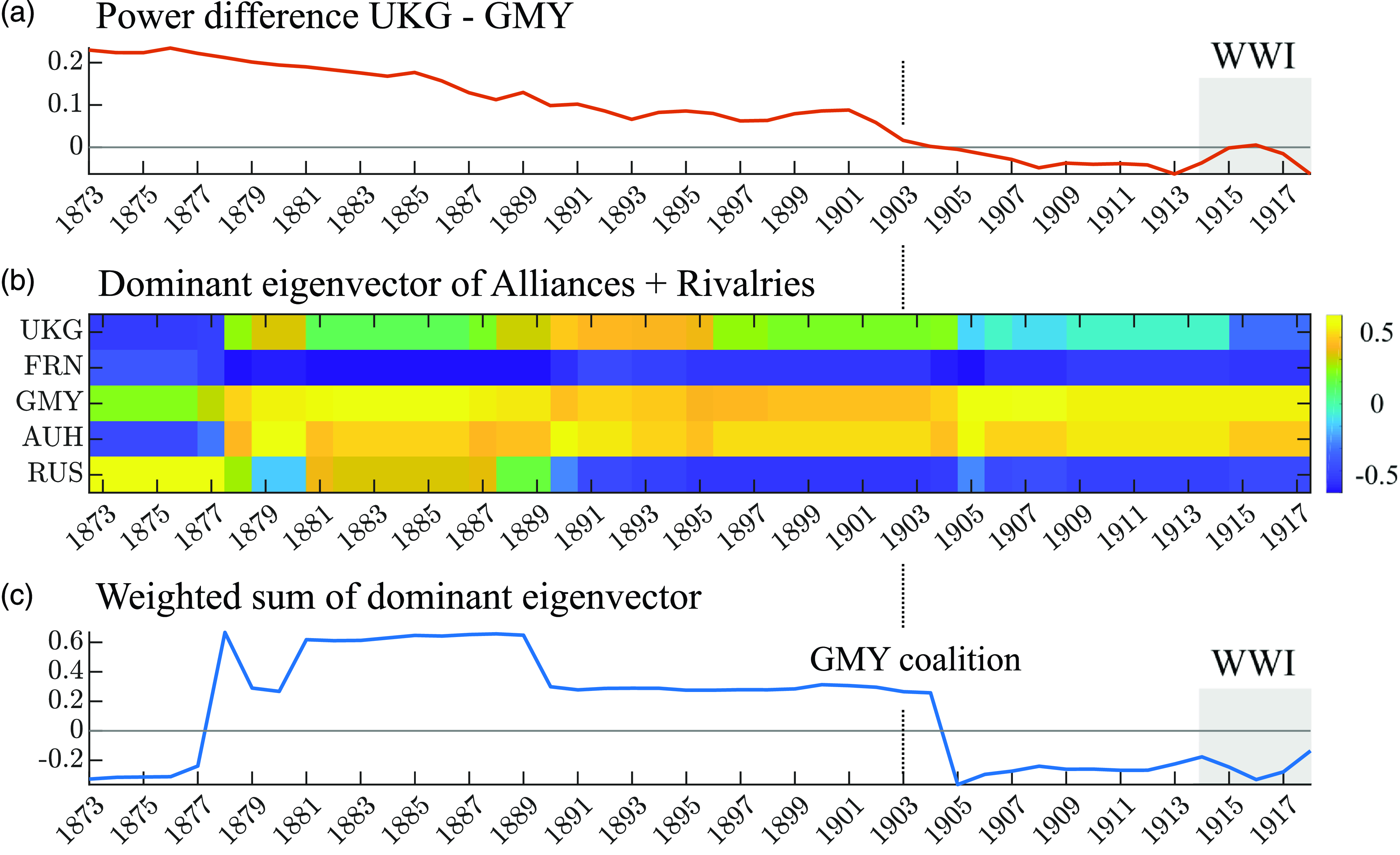
Figure 8. (a) Power difference between Great Britain and Germany. (b) Dominant eigenvector of the network of alliances and rivalries. (c) Sum of the dominant eigenvector weighted by relative power. Germany’s value in the eigenvector is always positive, meaning that positive sums indicate the German coalition is dominant while negative sums indicate the opposing coalition is dominant.
Although the First World War did not start when Figure 8(a) shows the power differential passing through zero in 1904, the war did start in 1914 when the differential was small, slightly in the anti-German coalition’s favor. In addition, the polarization of the system did increase in 1905 and some consider that the structural factors priming the system for war were already in place by then (Levy & Mulligan, Reference Levy and Mulligan2021). This is consistent with the fact that our model allows for war to be triggered in the bistable regime, prior to crossing the peace-to-war bifurcation threshold, as we discuss further below. Accordingly, the power differential can be viewed as a plausible driver for the balance sensitivity, particularly given the considerable empirical support that power transition theory has received (Rasler & Thompson, Reference Rasler and Thompson2010).
The perception among political and military leaders that offense dominates defense is another factor theorized as an important cause of systemic war (Van Evera, Reference Van1999). Paradoxically, although known for trench warfare and static front lines, World War I is the paradigmatic example of this perception. Despite some recognition of how recent technological developments in firepower had advanced defense, an offensive doctrine in which superior elan and morale were the keys to victory dominated military thought among the great powers prior to the war (Howard, Reference Howard1986). The belief that offense had the advantage fed the concern that, if a power left its ally unassisted when attacked by another great power, the ally would be quickly defeated, thereby leaving the power exposed to fight this belligerent alone (Christensen & Snyder, Reference Christensen and Snyder1990). This worry encouraged “chain ganging” in which the great powers bound themselves more tightly to their allies and concomitantly assumed more confrontational stances toward their friends’ foes. Conversely, a perceived advantage for defense loosens alliance commitments. Therefore, the extent to which warfare is viewed as favoring offense over defense, whether justified technologically or not, impacts structural balance pressures and so the offense-defense may be associated with the structural balance sensitivity.
Just as in the WWI case, the WWII factions emerge in the leading eigenvector prior to the start of the war. We observe the dominant structure in world powers leading up to World War II in Figure 9. Similar to the WWI analysis, we generate the pre-WWII network using the MIDs, alliances, and rivalries data from the Correlates of War dataset and the Handbook of International Rivalries (Palmer et al., 2015; Gibler, Reference Gibler2009; Singer & Small, Reference Singer and Small1966; Thompson & Dreyer, Reference Thompson and Dreyer2011). We find that the factions that formed during WWII (Allies versus Axis powers) arose in the network’s dominant eigenvector prior to the outbreak of the war (Figure 9(b)). The factions that became the Allied and Axis forces are present in the dominant eigenvector starting in 1936, three years prior to the start of WWII in 1939 (Figure 9(b)).Footnote 11 The dominant structure latent in the network prior to both WWI and WWII came to define the factions after conflict escalation. This is in agreement with our model’s prediction that a network’s dominant structure will be enhanced by structural balance forces and come to define the war state if the bifurcation point is reached.
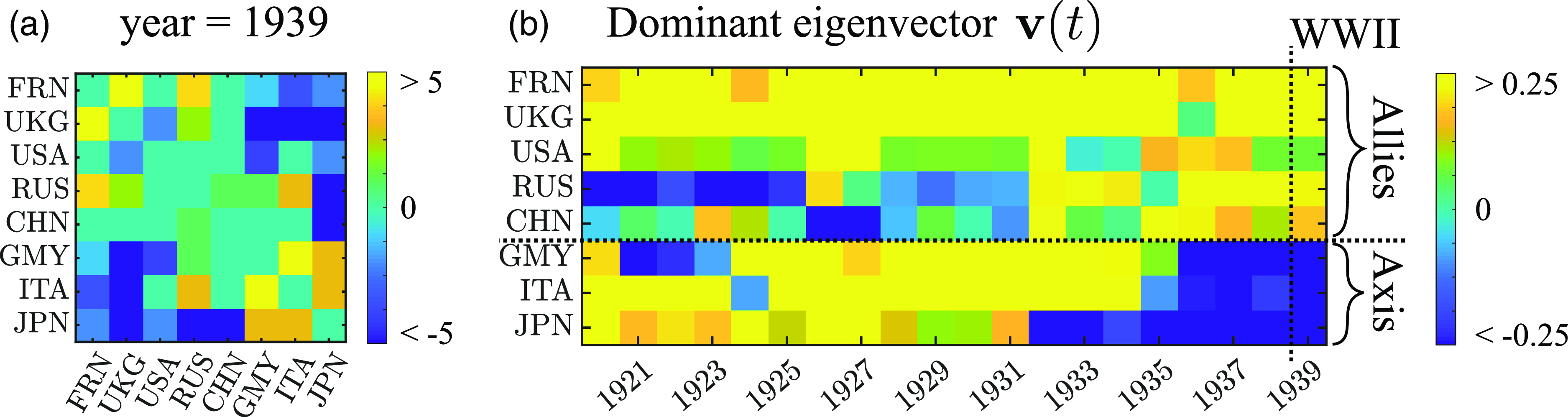
Figure 9. (a) Ties between countries in the year 1939—the beginning of WWII. Countries shown are the eight largest globally by CINC score. (b) Dominant eigenvector of the network leading up to WWII.
10.3 Bifurcation structure and the catalysts of war
The bifurcation structure of our model can be used to more precisely formulate the debate about the nature of the triggers of systemic wars. The unstable quality of the international system prior to structural wars has been likened to a powder keg and spark, in which the former signifies the systemic conditions creating the instability, while the latter represents the immediate episode triggering the war. The debate, which has been most keenly engaged for World War I, concerns whether the spark must be drawn from a narrow set of specific catalysts or, instead, a wider, more generic set. In favor of a narrow set, Lebow (Reference Lebow2000) and Levy and Mulligan (Reference Levy and Mulligan2021) argue that the onset of the First World War was highly contingent upon a crisis in the Balkans and, furthermore, upon the assassination of Archduke Franz Ferdinand, which removed the most influential voice of moderation in Austria-Hungary; if he had not been assassinated, the war might never have happened. On the other side, Thompson (Reference Thompson2003) subscribes to the “streetcar” view of the war: the structural factors destabilizing Europe were so intense that, like missing a streetcar, even if one crisis passed without sparking a war, another one would have come along sooner or later to do the job. In essence, these two views differ as to whether the war can be considered contingent or inevitable.
The bistable dynamics exhibited in our model can accommodate both generic and specific paths to war. The generic route essentially corresponds to the system having reached the peace-to-war bifurcation in which the peace equilibrium vanishes, leaving only war (as occurs at $\alpha ^*_{P \rightarrow W}$
in Figure 1(c)). Here, any perturbation will cause the system to go from peace to war. Actually, it would be more precise to say that the system is just shy of the bifurcation so that a wide range of small (but not infinitesimal) perturbations will destabilize it. Turning to the specific route, that corresponds to the system being firmly in the bistable zone where both the peace and war equilibria are possible (say at
$\alpha ^*_{P \rightarrow W}$
in Figure 1(c)). Here, any perturbation will cause the system to go from peace to war. Actually, it would be more precise to say that the system is just shy of the bifurcation so that a wide range of small (but not infinitesimal) perturbations will destabilize it. Turning to the specific route, that corresponds to the system being firmly in the bistable zone where both the peace and war equilibria are possible (say at $\alpha =0.03$
in Figure 1(c)), the system requires a substantially larger kick to jump from peace to war. The system, however, may be particularly vulnerable to specific perturbation patterns; for example, the pattern that fully counterposes the Franco-Russian and Austrian-German alliances minimizes the required energy (Figure 5(a)). If one sufficiently constrains the maximum size of a perturbation, then only a relatively narrow set of perturbations will shake the system into war. These most efficient perturbations then comprise the specific catalysts upon which war is contingent.
$\alpha =0.03$
in Figure 1(c)), the system requires a substantially larger kick to jump from peace to war. The system, however, may be particularly vulnerable to specific perturbation patterns; for example, the pattern that fully counterposes the Franco-Russian and Austrian-German alliances minimizes the required energy (Figure 5(a)). If one sufficiently constrains the maximum size of a perturbation, then only a relatively narrow set of perturbations will shake the system into war. These most efficient perturbations then comprise the specific catalysts upon which war is contingent.
Although the qualitative debate by necessity contrasts the war as either being inevitable or highly contingent, the model allows for a non-dichotomous formulation through use of the distance, in parameter space, from the peace-to-war bifurcation point. In the bistable zone, war onset is always considered to be contingent but the degree of contingency decreases as the system draws closer to the peace-to-war bifurcation point. In other words, the pool of destabilizing perturbations expands near the critical point. Note that, in the model, war is indeed inevitable beyond the peace-to-war bifurcation and, conversely, it is impossible prior to the war-to-peace bifurcation.
10.4 Empirically testing war as bifurcation
The most fundamental prediction arising from the model is that the transition from peace to war, whether via the generic or specific triggers, involves bifurcation structure. Remarkably, this prediction is amenable to empirical testing without the need to fit an explicit model to the data. This ability is a consequence of the universality of behavior for all systems in the vicinity of a given type of bifurcation, such as the saddle-node bifurcation displayed by our model. Critical transition theory identifies signatures associated with bifurcations, and critical slowing down in particular, such as increased variance, autocorrelations, and spatial correlations, longer recovery times, and power spectrum sharpening. These predictions involve not simply the direction of change in the signatures, but their quantitative scaling as a function of distance from the bifurcation (Kuehn, Reference Kuehn2011; Scheffer et al., Reference Scheffer, Carpenter, Lenton, Bascompte, Brock, Dakos and Vandermeer2012; Meisel et al., Reference Meisel, Klaus, Kuehn and Plenz2015; Bury et al., Reference Bury, Bauch and Anand2020).
Our preliminary look at the recovery rate response to militarized interstate disputes among the five great powers in the decades prior to World War I did not find evidence of critical slowing down. However, consistent with critical slowing down, Midlarsky (Reference Midlarsky1984, Reference Midlarsky1986) theorized that as the onset of war grows closer, disputes would take longer to resolve and hence accumulate, finding evidence for such accumulation prior to World War I. Importantly, disputes involving lesser powers formed a critical part of his theory and findings. This suggests that future research on critical slowing down in international relations should involve wider networks beyond the great powers.
Given these mechanisms for destabilization, the formation of new alliances, increased connectivity, the addition of more countries to a system, or fluctuations in relative power could all increase the instability in a system of states and lead to systemic war. While at the dyadic level, forming new connections may not add much conflict to a system or be detrimental for the parties involved, it could inadvertently make a system less stable by allowing for more nonlinear interactions between edges, increasing community structure, or equalizing a power imbalance. Dynamical system models, such as the one introduced here, may be useful in assessing how changes to ties impact not only the countries involved but the entire system; models for system-wide impact could be beneficial in assessing systemic risk and designing de-escalation strategies.
11. Conclusion
We have presented a model of the dynamics of cooperation and conflict that integrates complex systems and complex network approaches. Our work makes contact with elements of complex systems theory including nonlinear dynamics, bifurcations, stability analysis, and critical transition signatures. With respect to complex networks, our work involves signed networks, structural balance theory, and community structure. Spectral decomposition into eigenvalues and eigenvectors, and in particular the dimension reduction so afforded, provides a unifying framework for both the complex systems and networks aspects, allowing for calculation of bifurcation conditions, the compact representation of dominant polarized community structure, and empirical application to great power politics.
In our model, the tie value between two nodes evolves under the influence of a direct dyadic force biasing the nodes toward a low-level equilibrium, and a structural balance force, which shifts the nodes toward greater cooperation or conflict if they have similar or dissimilar relationships with mutual neighbors. We focused on the situation when the dyadic bias matrix can give rise to two possible stable equilibrium states: a peace state of low-level conflict and cooperation in which the equilibrium tie values are near their dyadic biases and a war state of high-level conflict and cooperation. Varying the structural balance sensitivity, which determines how sharply the balance force increases or decreases around the neutral point, then results in three regimes: a monostable peace state, a bistable regime where both peace and war states exist, and a monostable war state. Saddle-node bifurcations mark the transitions between these regimes. The sandwiching of the bistable regime between the peace and war monostable regimes results in a form of path dependence known as hysteresis: as the balance sensitivity is increased and then decreased past the peace-to-war bifurcation, the system does not return back down to the peace state at the same value it transitioned up to the war state, but rather a lower one.
We used our model to investigate structural features that make systemic war in a network more likely and identify patterns of perturbations that have the most impact on system stability. We derived approximate analytical solutions for the bifurcation conditions in both a special case and generally, which reveal the key role of the first eigenvalue of the dyadic bias matrix. This enabled us to show how polarized community structure as contained in the first eigenvector makes the network more prone to systemic war by lowering the critical balance sensitivity at which the peace-to-war bifurcation occurs. This finding concords with theory emphasizing the destabilization effects of alliance polarization, but is also generalizable to structural features beyond polarization via the impact of those features on the first eigenvalue.
When the system is in the bistable regime, we considered the ability of finite, transient perturbations to induce a transition from peace to war. The most destabilizing perturbation pattern is constructed from the first eigenvector of the dyadic bias matrix. We also developed a scheme to find other destabilizing perturbations of low energy. We illustrated the empirical application of this perturbation analysis framework on the great power network immediately prior to World War I. The minimum energy perturbation excited cooperation and conflict, respectively, within and between the alliances involving the four Continental powers but not Great Britain. This pattern is consistent with the strong commitments exhibited within the Continental alliances in the crisis that triggered the war while Britain took a more ambiguous stance even though it was allied with France and Russia.
There are many empirical avenues for future research to build upon this work. The model’s prediction of war as bifurcation could be tested via a systematic search for critical slowing down behaviors. The linkage between network structure and greater risk of systemic war could be found in network spectra as the emergence from the main spectral band of a polarized first eigenvector. Another line of empirical investigation would endeavor to identify variables in the international system that affect structural balance pressures, which could involve testing their correlation with a metric of structural balance (Kirkley et al., Reference Kirkley, Cantwell and Newman2019; Burghardt & Maoz, Reference Burghardt and Maoz2020). Although our substantive focus here has been international relations between states, other contexts involving cooperation and conflict driven by both dyad-specific and structural balance dynamics could serve as testing grounds, such as fragmented civil wars in which a multiplicity of armed groups fight and ally with each other.
We note a few ways in which the model can be extended. The products of the ties in the structural balance sum could be weighted by power so that powerful nodes contribute more to it than weaker ones. The ties could also be made directed to represent asymmetric relationships of aid or aggression. Other mechanisms influencing tie dynamics beyond the dyadic and structural balance forces could be incorporated into the model. One significant force that is not currently represented is power balancing dynamics in which state alliance decisions are driven by power calculations rather than existing alliances or enmities as in structural balance. States may ally with an erstwhile adversary to balance against a looming threat from an aggressive power. They may also abandon an existing ally to bandwagon with a powerful aggressor (Walt, Reference Walt1990). As maintaining the balance of power has long been claimed to be crucial to sustaining equilibrium in the international system, (Healy & Stein, Reference Healy and Stein1973; Kissinger, Reference Kissinger1994; Rasler & Thompson, Reference Rasler and Thompson2010), incorporating both power balancing and structural dynamics within the same model could be a fruitful way of better understanding how they interact to produce peace and war.
While this paper has concentrated on destabilizing factors and perturbations that make systemic war more likely, the model also has implications for preventing war and transitioning from war to peace. One example is that a perturbation pattern opposite to that calculated above as most dangerous will most efficiently keep the system from destabilizing. Another is that, in the bistable regime, optimal perturbations for kicking the system from the war to the peace state can be calculated rather than the reverse direction we treated herein. Alternatively, lowering the balance sensitivity beneath its critical value for the war-to-peace bifurcation would yield a monostable peace state. If the balance sensitivity were related to a power differential between key states, then increasing its war-to-peace critical value would correspond to lowering the power disparity at which peace is restored, implying that the losing side need not be defeated as decisively to bring the war to an end; Equation (6) shows that decreasing the first eigenvalue of the bias network would have that effect. Finally, although it still lies in the realm of political philosophy and prophetic visions (at least for the international system), the model also possesses an equilibrium of high-level universal cooperation, the harmony state, which can be reached from both the peace and war states.
Acknowledgements
We thank the anonymous referees for their helpful feedback and Olga Chyzh for pointing us to relevant literature.
Competing interests
None.
Funding statement
This work was supported by the National Science Foundation (MM, award no. 2103239); the Army Research Office (MM and MG, grant no. W911NF1910291); and the Air Force Office of Scientific Research (JNK, grant no. FA9550-17-1-0329).
Data availability statement
Replication code for select figures is available at https://github.com/mmtree/Transitions_between_peace_and_systemic_war.
Appendix A. General treatment
We provide the derivations of the approximate bifurcation conditions stated in Section 5.2 for a general dyadic bias matrix.
A.1 Approximate system
We replace the full matrix dynamical system, Equation (16), with analytically tractable forms by using approximations for the hyperbolic tangent function in the transition and plateau regions. In the transition region, $\theta =(\alpha/ L) \textbf{X}^2 \ll 1$
, using
$\theta =(\alpha/ L) \textbf{X}^2 \ll 1$
, using $\tanh \theta \approx \theta$
yields
$\tanh \theta \approx \theta$
yields
 \begin{align} \frac{d\textbf{X}}{dt} = -\beta (\textbf{X} - \textbf{X}_D) + \alpha \textbf{X}^2 + \textbf{X}_T(t) \end{align}
This system has approximately the same stable peace and unstable fixed points as Equation (16) for large $L$
, but does not have the stable war fixed point. Because the unstable fixed points of Equation (A1) approach the unstable fixed points of Equation (16) as
$L$
, but does not have the stable war fixed point. Because the unstable fixed points of Equation (A1) approach the unstable fixed points of Equation (16) as $L \rightarrow \infty$
, theoretical results derived from Equation (A1) are less accurate for smaller
$L \rightarrow \infty$
, theoretical results derived from Equation (A1) are less accurate for smaller $L$
values.
$L$
values.
In the plateau region, $|\theta | \gg 1$
, we use
$|\theta | \gg 1$
, we use $\tanh \theta \approx \pm 1$
to yield
$\tanh \theta \approx \pm 1$
to yield
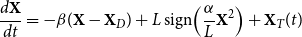 \begin{align} \frac{d\textbf{X}}{dt} = -\beta (\textbf{X} - \textbf{X}_D) + L\;\text{sign}\!\left({\frac{\alpha }{L}\textbf{X}^2}\right) + \textbf{X}_T(t) \end{align}
where the use of $\text{sign}(\alpha{\textbf{X}^2}/L)$
assumes that all the components of
$\text{sign}(\alpha{\textbf{X}^2}/L)$
assumes that all the components of $\textbf{X}^2$
are sufficiently large to be approximated as being on the positive or negative plateaus. We furthermore assume that
$\textbf{X}^2$
are sufficiently large to be approximated as being on the positive or negative plateaus. We furthermore assume that $\text{sign}({\textbf{X}^2})$
can be approximated using the signs of the components of the first eigenvector of
$\text{sign}({\textbf{X}^2})$
can be approximated using the signs of the components of the first eigenvector of $\textbf{X}$
,
$\textbf{X}$
, $\textbf{s}_1$
. Denoting the vector of signs as
$\textbf{s}_1$
. Denoting the vector of signs as $\textbf{u}$
, we then have
$\textbf{u}$
, we then have $\textbf{u} = \text{sign}(\textbf{s}_1)$
. We can then replace
$\textbf{u} = \text{sign}(\textbf{s}_1)$
. We can then replace $\text{sign}(\alpha{\textbf{X}^2/L})$
by
$\text{sign}(\alpha{\textbf{X}^2/L})$
by $\textbf{u}\textbf{u}^T$
in Equation (A2) yielding
$\textbf{u}\textbf{u}^T$
in Equation (A2) yielding
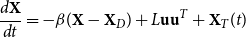 \begin{align} \frac{d\textbf{X}}{dt} = -\beta (\textbf{X} - \textbf{X}_D) + L\textbf{u}\textbf{u}^T + \textbf{X}_T(t) \end{align}
This approximation is valid for $L$
sufficiently large so that, for trajectories heading from the peace state of low tie values to a high tie value equilibrium, the feed-forward growth has time to preferentially amplify the leading eigenvector
$L$
sufficiently large so that, for trajectories heading from the peace state of low tie values to a high tie value equilibrium, the feed-forward growth has time to preferentially amplify the leading eigenvector $\textbf{s}_1$
, similar to the behavior in the pure structural balance model of Equation (2).
$\textbf{s}_1$
, similar to the behavior in the pure structural balance model of Equation (2).
A.2 Stable and unstable fixed points
We now find fixed points of the approximate system in the transition region, Equation (A1), in the absence of the transient term ( $\textbf{X}_T=0$
) by expressing it in terms of the dynamics of its eigenvalues and eigenvectors. We denote the tie matrix at a fixed point by
$\textbf{X}_T=0$
) by expressing it in terms of the dynamics of its eigenvalues and eigenvectors. We denote the tie matrix at a fixed point by $\textbf{X}_0$
and write its eigenvector decomposition as
$\textbf{X}_0$
and write its eigenvector decomposition as $\textbf{X}_0 = \textbf{S}_0 \Lambda _0 \textbf{S}_0^T$
and that of the dyadic bias matrix as
$\textbf{X}_0 = \textbf{S}_0 \Lambda _0 \textbf{S}_0^T$
and that of the dyadic bias matrix as $\textbf{X}_D = \textbf{S}_D \Lambda _D \textbf{S}_D^T$
. For simplicity, we assume that
$\textbf{X}_D = \textbf{S}_D \Lambda _D \textbf{S}_D^T$
. For simplicity, we assume that $\textbf{X}_0$
and
$\textbf{X}_0$
and $\textbf{X}_D$
are full-rank matrices, allowing us to perform an eigendecomposition. Setting
$\textbf{X}_D$
are full-rank matrices, allowing us to perform an eigendecomposition. Setting $\frac{d\textbf{X}}{dt} = 0$
, using these decompositions, and rearranging yields
$\frac{d\textbf{X}}{dt} = 0$
, using these decompositions, and rearranging yields
 \begin{align} 0 &= -\beta \!\left (\textbf{X}_0 - \textbf{X}_D \right ) + \alpha \textbf{X}_0^2 \end{align}
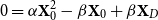 \begin{align} 0 &= \alpha \textbf{X}_0^2 -\beta \textbf{X}_0 + \beta \textbf{X}_D \end{align}
 \begin{align} 0 &= \alpha \textbf{S}_0 \Lambda _0^2 \textbf{S}_0^T -\beta \textbf{S}_0 \Lambda _0 \textbf{S}_0^T + \beta \textbf{S}_D \Lambda _D \textbf{S}_D^T \end{align}
 \begin{align} \textbf{S}_0(\alpha \Lambda _0^2 -\beta \Lambda _0) \textbf{S}_0^T &= - \beta \textbf{S}_D \Lambda _D \textbf{S}_D^T \end{align}
where we have used the orthonormality of the eigenvectors, $\textbf{S}_0^T \textbf{S}_0 = I$
in the third line.
$\textbf{S}_0^T \textbf{S}_0 = I$
in the third line.
We diagonalize the left-hand side by multiplying by $\textbf{S}_0^T$
and
$\textbf{S}_0^T$
and $\textbf{S}_0$
on the left and right, respectively,
$\textbf{S}_0$
on the left and right, respectively,
 \begin{align} \alpha \Lambda _0^2 -\beta \Lambda _0 &= - \beta \textbf{S}_0^T\textbf{S}_D \Lambda _D \textbf{S}_D^T \textbf{S}_0 \end{align}
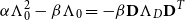 \begin{align} \alpha \Lambda _0^2 -\beta \Lambda _0 &= - \beta \textbf{D} \Lambda _D \textbf{D}^T \end{align}
where $\textbf{D} = \textbf{S}_0^T\textbf{S}_D$
. Since the left-hand side is diagonal then the right-hand side must also be diagonal. Because
$\textbf{D} = \textbf{S}_0^T\textbf{S}_D$
. Since the left-hand side is diagonal then the right-hand side must also be diagonal. Because $\textbf{S}_0$
and
$\textbf{S}_0$
and $\textbf{S}_D$
are orthonormal matrices, these diagonal values generated by the inner product
$\textbf{S}_D$
are orthonormal matrices, these diagonal values generated by the inner product $\textbf{s}_{0i}^T \textbf{s}_{Di}$
must be equal to 1. Therefore,
$\textbf{s}_{0i}^T \textbf{s}_{Di}$
must be equal to 1. Therefore, $\textbf{D}$
must be the identity matrix,
$\textbf{D}$
must be the identity matrix, $\textbf{S}_0^T\textbf{S}_D = I$
. Therefore,
$\textbf{S}_0^T\textbf{S}_D = I$
. Therefore, $\textbf{S}_0 = \textbf{S}_D$
. This implies that the eigenvectors of
$\textbf{S}_0 = \textbf{S}_D$
. This implies that the eigenvectors of $\textbf{X}_0$
are the same as the eigenvectors of
$\textbf{X}_0$
are the same as the eigenvectors of $\textbf{X}_D$
. This allows us to diagonalize the matrix dynamical system equation at the fixed points and solve for the eigenvalues of
$\textbf{X}_D$
. This allows us to diagonalize the matrix dynamical system equation at the fixed points and solve for the eigenvalues of $\textbf{X}$
there. As the right-hand side of (A9) simplifies to
$\textbf{X}$
there. As the right-hand side of (A9) simplifies to $-\beta \Lambda _D$
, we rearrange to obtain
$-\beta \Lambda _D$
, we rearrange to obtain
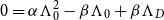 \begin{align} 0 &= \alpha \Lambda _0^2 -\beta \Lambda _0 + \beta \Lambda _D \end{align}
which expressed in terms of the individual eigenvalues $\lambda _{0i}$
is
$\lambda _{0i}$
is
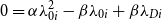 \begin{align} 0 &= \alpha \lambda _{0i}^2 -\beta \lambda _{0i} + \beta \lambda _{Di} \end{align}
Solving yields
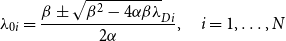 \begin{align} \lambda _{0i} &= \frac{\beta \pm \sqrt{\beta ^2 - 4\alpha \beta \lambda }_{Di}}{2 \alpha },\quad i = 1,\ldots,N \end{align}
for the fixed point eigenvalues. Eigenvalues of the stable fixed point are given by the negative sign and those of the unstable fixed point by the positive sign as we now show.
For a stable fixed point, small perturbations will decay, whereas they will grow for an unstable fixed point. The response is given by the eigenvalues of the linearized system. Denoting the perturbation by $\boldsymbol{\delta}\boldsymbol{{X}}$
, the linearized system is
$\boldsymbol{\delta}\boldsymbol{{X}}$
, the linearized system is
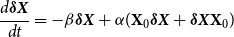 \begin{align} \frac{d \boldsymbol{\delta}\boldsymbol{{X}}}{dt} &= -\beta \boldsymbol{\delta}\boldsymbol{{X}} + \alpha (\textbf{X}_0 \boldsymbol{\delta}\boldsymbol{{X}} + \boldsymbol{\delta}\boldsymbol{{X}} \textbf{X}_0) \end{align}
Using the above result that the eigenvectors of $\textbf{X}_0$
are the same as
$\textbf{X}_0$
are the same as $\textbf{X}_D$
, we expand the fixed point and the perturbation in terms of the eigenvectors,
$\textbf{X}_D$
, we expand the fixed point and the perturbation in terms of the eigenvectors, $\textbf{s}_D$
, so that
$\textbf{s}_D$
, so that $\textbf{X}_0 = \sum _{i=1}^N \lambda _{0i} \textbf{s}_{Di}\textbf{s}_{Di}^T$
and
$\textbf{X}_0 = \sum _{i=1}^N \lambda _{0i} \textbf{s}_{Di}\textbf{s}_{Di}^T$
and $\boldsymbol{\delta}\boldsymbol{{X}}_0 = \sum _{i=1}^N a_i(t) \textbf{s}_{Di}\textbf{s}_{Di}^T$
, where
$\boldsymbol{\delta}\boldsymbol{{X}}_0 = \sum _{i=1}^N a_i(t) \textbf{s}_{Di}\textbf{s}_{Di}^T$
, where $a_i(t)$
is the time-dependent amplitude of the
$a_i(t)$
is the time-dependent amplitude of the $i^{th}$
mode. Using these expansions in Equation (A13), we find that each mode evolves independently via
$i^{th}$
mode. Using these expansions in Equation (A13), we find that each mode evolves independently via
 \begin{align} \frac{d a_i}{dt} &= \!\left (-\beta + 2\alpha \lambda _{0i}\right ) a_i \end{align}
Taking the modes to have an exponential time dependence, $a_i \sim e^{\nu _i t}$
, the growth rate
$a_i \sim e^{\nu _i t}$
, the growth rate $\nu _i$
is given by
$\nu _i$
is given by
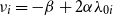 \begin{align} \nu _i &= -\beta + 2\alpha \lambda _{0i} \end{align}
Substituting for $\lambda _{0i}$
using (A12) then gives
$\lambda _{0i}$
using (A12) then gives
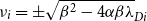 \begin{align} \nu _i &= \pm \sqrt{\beta ^2 - 4\alpha \beta \lambda }_{Di} \end{align}
The positive and negative signs in Equation (A12) therefore correspond, respectively, to growing and decaying perturbations and so are associated with the unstable and stable fixed points as claimed above.
The stable fixed point corresponds to the peace state and its leading eigenvalue $\lambda _P$
is given by
$\lambda _P$
is given by
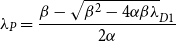 \begin{align} \lambda _P = \frac{\beta - \sqrt{\beta ^2 - 4\alpha \beta \lambda }_{D1}}{2 \alpha } \end{align}
For the unstable fixed point, the leading eigenvalue is not of concern but rather the lowest one,
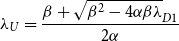 \begin{align} \lambda _U &= \frac{\beta + \sqrt{\beta ^2 - 4\alpha \beta \lambda }_{D1}}{2 \alpha } \end{align}
as the peace-to-war bifurcation occurs when it equals $\lambda _P$
.
$\lambda _P$
.
The case when a finite, transient perturbation, $\textbf{X}_T(t)$
, is applied to the system can be treated similarly if we take it to have the form of an impulse where all its elements are constant over the duration of the transient. Defining the modified dyadic bias matrix,
$\textbf{X}_T(t)$
, is applied to the system can be treated similarly if we take it to have the form of an impulse where all its elements are constant over the duration of the transient. Defining the modified dyadic bias matrix, $\tilde{\textbf{X}}_D(t) = \textbf{X}_D + \textbf{X}_T(t)/\beta$
, we can rewrite Equation (A1) as
$\tilde{\textbf{X}}_D(t) = \textbf{X}_D + \textbf{X}_T(t)/\beta$
, we can rewrite Equation (A1) as
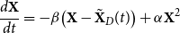 \begin{align} \frac{d\textbf{X}}{dt} &= -\beta \!\left (\textbf{X} - \tilde{\textbf{X}}_D(t) \right ) + \alpha \textbf{X}^2 \end{align}
This modification in dyadic biases results in a new effective peace state eigenvalue given by
 \begin{align} \lambda _P = \frac{\beta - \sqrt{\beta ^2 - 4\alpha \beta \tilde{\lambda }_{D1}(t)}}{2 \alpha } \end{align}
Similarly, the lowest eigenvalue of the unstable state becomes
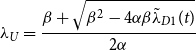 \begin{align} \lambda _U &= \frac{\beta + \sqrt{\beta ^2 - 4\alpha \beta \tilde{\lambda }_{D1}(t)}}{2 \alpha } \end{align}
If the perturbation is sufficiently small, then $\lambda _P$
and
$\lambda _P$
and $\lambda _U$
will be real and nonzero. The corresponding fixed points will exist, and, in particular, the system will settle into a new peace state as shifted by the perturbation, assuming that the transient duration is long enough. A large perturbation, however, can cause the square root in (A20) and (A21) to be imaginary, in which case the stable and unstable fixed points do not exist; the system will head toward a stable equilibrium of high conflict and/or cooperation as we now discuss.
$\lambda _U$
will be real and nonzero. The corresponding fixed points will exist, and, in particular, the system will settle into a new peace state as shifted by the perturbation, assuming that the transient duration is long enough. A large perturbation, however, can cause the square root in (A20) and (A21) to be imaginary, in which case the stable and unstable fixed points do not exist; the system will head toward a stable equilibrium of high conflict and/or cooperation as we now discuss.
We calculate the high conflict and cooperation fixed points using the plateau approximation of the dynamics as given by Equation (A3). Setting $\frac{d\textbf{X}}{dt}=0$
and solving for the fixed point
$\frac{d\textbf{X}}{dt}=0$
and solving for the fixed point $\textbf{X}_0$
produces
$\textbf{X}_0$
produces
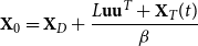 \begin{align} \textbf{X}_0 &= \textbf{X}_D + \frac{L \textbf{u}\textbf{u}^T + \textbf{X}_T(t)}{\beta } \end{align}
When no transient perturbation is applied, the stable state which results from the peace-to-war bifurcation will be the war state as determined by the leading eigenvector of $\textbf{X}_D$
and we write the sign vector as
$\textbf{X}_D$
and we write the sign vector as $\textbf{u}_{D1}=\text{sign}(\textbf{s}_{D1})$
. The war state in the plateau approximation is then given by
$\textbf{u}_{D1}=\text{sign}(\textbf{s}_{D1})$
. The war state in the plateau approximation is then given by
 \begin{align} \textbf{X}_W &= \textbf{X}_D + \frac{L}{\beta } \textbf{u}_{D1}\textbf{u}_{D1}^T \end{align}
When an applied perturbation does shift the system out of the peace state, the first eigenvector, $\tilde{\textbf{s}}_{D1}$
, of the modified dyadic bias matrix will grow to dominate the network if
$\tilde{\textbf{s}}_{D1}$
, of the modified dyadic bias matrix will grow to dominate the network if $L/\beta$
is large in comparison with
$L/\beta$
is large in comparison with $||\tilde{\textbf{X}}_D||$
. In this case, after the perturbation has ended, the final high tie value state of the system,
$||\tilde{\textbf{X}}_D||$
. In this case, after the perturbation has ended, the final high tie value state of the system, $\textbf{X}_H$
, will be approximately
$\textbf{X}_H$
, will be approximately
 \begin{align} \textbf{X}_H &= \frac{L}{\beta } \tilde{\textbf{u}}_{D1}\tilde{\textbf{u}}_{D1}^T \end{align}
where $\tilde{\textbf{u}}_{D1}=\text{sign}(\tilde{\textbf{s}}_{D1})$
. This expression was used to calculate the final states in Figure 5. However, if
$\tilde{\textbf{u}}_{D1}=\text{sign}(\tilde{\textbf{s}}_{D1})$
. This expression was used to calculate the final states in Figure 5. However, if $L$
is not large enough to provide enough time for
$L$
is not large enough to provide enough time for $\tilde{\textbf{u}}_{D1}$
to grow to dominate the network, the final network structure will have noticeable contributions from other eigenvectors of
$\tilde{\textbf{u}}_{D1}$
to grow to dominate the network, the final network structure will have noticeable contributions from other eigenvectors of $\tilde{\textbf{X}}_D$
.
$\tilde{\textbf{X}}_D$
.
A.3 Bifurcation transition from peace to war
The peace-to-war transition occurs when the first eigenvalue of the linearized system at the peace state is zero, corresponding to a saddle-node bifurcation. Setting $\nu _1=-\sqrt{\beta ^2 - 4\alpha \beta \lambda }_{D1}$
to zero and solving for the critical balance sensitivity yields
$\nu _1=-\sqrt{\beta ^2 - 4\alpha \beta \lambda }_{D1}$
to zero and solving for the critical balance sensitivity yields
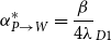 \begin{align} \alpha ^*_{P\rightarrow W} = \frac{\beta }{4 \lambda }_{D1} \end{align}
The vanishing of the discriminant in Equation (A17) yields the critical value of the peace state eigenvalue at the bifurcation,
 \begin{align} \lambda _{P}^* = \frac{\beta }{2 \alpha ^*_{P \rightarrow W}} \end{align}
Equation (A18) shows that the unstable state eigenvalue also has this value at the bifurcation so that $\lambda _P^* = \lambda _U^*$
. This equality of the stable and unstable critical eigenvalues corresponds to the merging of the stable and unstable fixed points that occurs in a saddle-node bifurcation.
$\lambda _P^* = \lambda _U^*$
. This equality of the stable and unstable critical eigenvalues corresponds to the merging of the stable and unstable fixed points that occurs in a saddle-node bifurcation.
For the case where the impulse perturbation $\textbf{X}_T$
is applied to the peace equilibrium
$\textbf{X}_T$
is applied to the peace equilibrium $\textbf{X}_P$
, the system parameters
$\textbf{X}_P$
, the system parameters $\alpha$
and
$\alpha$
and $\beta$
are fixed and we seek the critical eigenvalue,
$\beta$
are fixed and we seek the critical eigenvalue, $\tilde{\lambda }_{D1}^*$
, of the modified dyadic bias matrix
$\tilde{\lambda }_{D1}^*$
, of the modified dyadic bias matrix $\tilde{\textbf{X}}_D$
. This will occur when the effective peace and unstable eigenvalues due to the perturbation are equal. This yields a condition analogous to (A25) but which we express in terms of the critical eigenvalue,
$\tilde{\textbf{X}}_D$
. This will occur when the effective peace and unstable eigenvalues due to the perturbation are equal. This yields a condition analogous to (A25) but which we express in terms of the critical eigenvalue,
 \begin{align} \tilde{\lambda }_{D1}^* &= \frac{\beta }{4 \alpha } \end{align}
If ${\tilde{\lambda}_{{D1}}} \gt \tilde{\lambda }_{D1}^*$
, then the perturbation will kick the system out of the peace state into a high conflict and cooperation state.
${\tilde{\lambda}_{{D1}}} \gt \tilde{\lambda }_{D1}^*$
, then the perturbation will kick the system out of the peace state into a high conflict and cooperation state.
A.4 Bifurcation transition from war to peace
We consider the bifurcation from the war state, $\textbf{X}_W$
, back to the peace state as illustrated in the hysteresis curve of Figure 1(c). No external perturbation is imposed in this case (
$\textbf{X}_W$
, back to the peace state as illustrated in the hysteresis curve of Figure 1(c). No external perturbation is imposed in this case ( $\textbf{X}_T=0$
). Equation (A23) shows that the war state is the sum of
$\textbf{X}_T=0$
). Equation (A23) shows that the war state is the sum of $\textbf{X}_D$
and a rank-one matrix. We therefore approximate
$\textbf{X}_D$
and a rank-one matrix. We therefore approximate $\lambda _W$
by the expression for the upper bound of the leading eigenvalue of the sum of a symmetric matrix and a rank-one modification (Bunch et al., Reference Bunch, Nielsen and Sorensen1978),
$\lambda _W$
by the expression for the upper bound of the leading eigenvalue of the sum of a symmetric matrix and a rank-one modification (Bunch et al., Reference Bunch, Nielsen and Sorensen1978),
 \begin{align} \lambda _W = \lambda _{D1} + \frac{L N}{\beta } \end{align}
Note that increasing the size of the network as well as $L/\beta$
increases
$L/\beta$
increases $\lambda _W$
. A larger
$\lambda _W$
. A larger $\lambda _{D1}$
has similar effect implying that a polarized peace state is not only more susceptible to war (Section 6) but results in more intense conflict should that war arise.
$\lambda _{D1}$
has similar effect implying that a polarized peace state is not only more susceptible to war (Section 6) but results in more intense conflict should that war arise.
The transition from the war to the peace state is also generated by a saddle-node bifurcation, one distinct from the peace-to-war transition. The war-to-peace bifurcation occurs when the stable war fixed point and the unstable fixed point collide, leaving only the stable peace state as the remaining equilibrium. Given that our approximate dynamical systems in the transition and plateau regions do not mesh smoothly, we cannot perform a linear stability analysis for the war state (which is always stable in the plateau approximation) as we did for the peace state. However, we can make a rough calculation of the bifurcation condition by setting $\lambda _W$
equal to
$\lambda _W$
equal to $\lambda _U$
from Equation (A18). Doing so and solving for the critical balance sensitivity yields
$\lambda _U$
from Equation (A18). Doing so and solving for the critical balance sensitivity yields
 \begin{align} \lambda _{D1} + \frac{L N}{\beta } &= \frac{\beta + \sqrt{\beta ^2 - 4\alpha \beta \lambda _{D1}}}{2 \alpha } \end{align}
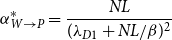 \begin{align} \alpha ^*_{W\rightarrow P} &= \frac{NL}{(\lambda _{D1} + NL/\beta )^2} \end{align}
Thus, for $L/\beta$
large, the transition back from war to peace will take place at a much lower
$L/\beta$
large, the transition back from war to peace will take place at a much lower $\alpha$
value than for the transition from peace to war, Equation (A25).
$\alpha$
value than for the transition from peace to war, Equation (A25).
Figure A1 visualizes the bifurcation structure of our system as approximated by the dynamics of the first eigenvalue, $\lambda _1(t)$
, under the expansion of the network by the dyadic bias matrix eigenvectors,
$\lambda _1(t)$
, under the expansion of the network by the dyadic bias matrix eigenvectors, $\textbf{X}(t)=\sum _k \lambda _i(t) \textbf{s}_{Dk} \textbf{s}_{Dk}^T$
. Its rate of change,
$\textbf{X}(t)=\sum _k \lambda _i(t) \textbf{s}_{Dk} \textbf{s}_{Dk}^T$
. Its rate of change, $d\lambda _1/dt$
, is plotted as a function of
$d\lambda _1/dt$
, is plotted as a function of $\lambda _1$
for the transition and plateau approximations (dotted curves) for which the modes evolve independently. Also shown is as a smooth approximation that retains the hyperbolic tangent (solid curve). Points where
$\lambda _1$
for the transition and plateau approximations (dotted curves) for which the modes evolve independently. Also shown is as a smooth approximation that retains the hyperbolic tangent (solid curve). Points where $d\lambda _1/dt=0$
correspond to fixed points and the arrows indicate their stability. Figure A1(a) shows the bistable regime in which
$d\lambda _1/dt=0$
correspond to fixed points and the arrows indicate their stability. Figure A1(a) shows the bistable regime in which $\lambda _1$
is stable at
$\lambda _1$
is stable at $\lambda _P$
and at
$\lambda _P$
and at $\lambda _W$
, with the unstable fixed point residing between them. For an increased value of
$\lambda _W$
, with the unstable fixed point residing between them. For an increased value of $\lambda _{D1}$
, Figure A1(b) shows the saddle-node bifurcation point corresponding to the peace-to-war transition in which
$\lambda _{D1}$
, Figure A1(b) shows the saddle-node bifurcation point corresponding to the peace-to-war transition in which $\lambda _P$
and
$\lambda _P$
and $\lambda _U$
have merged. The other saddle-node bifurcation, in which
$\lambda _U$
have merged. The other saddle-node bifurcation, in which $\lambda _U$
merges with
$\lambda _U$
merges with $\lambda _W$
, is shown in Figure A1(c) and corresponds to the war-to-peace transition when
$\lambda _W$
, is shown in Figure A1(c) and corresponds to the war-to-peace transition when $\alpha$
is decreased.
$\alpha$
is decreased.
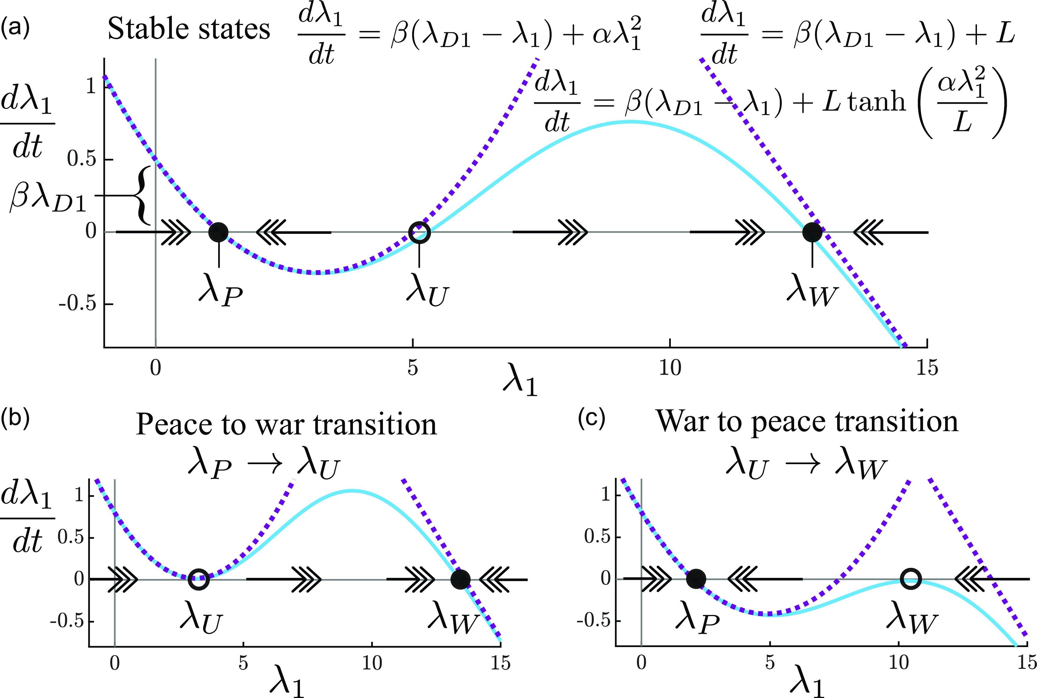
Figure A1. (a) Dynamics of the leading eigenvalue as a function of initial conditions. $\lambda _P$
and
$\lambda _P$
and $\lambda _W$
are stable fixed points separated by an unstable fixed point
$\lambda _W$
are stable fixed points separated by an unstable fixed point $\lambda _U$
. Curves approximate the eigenvalue dynamics.
$\lambda _U$
. Curves approximate the eigenvalue dynamics. $\alpha =0.08$
,
$\alpha =0.08$
, $\beta = 0.5$
,
$\beta = 0.5$
, $L = 6$
, and
$L = 6$
, and $\lambda _{D1} = 1$
. (b) A saddle-node bifurcation of the stable and unstable fixed points
$\lambda _{D1} = 1$
. (b) A saddle-node bifurcation of the stable and unstable fixed points $\lambda _P$
and
$\lambda _P$
and $\lambda _U$
underlies the peace-to-war transition.
$\lambda _U$
underlies the peace-to-war transition. $\alpha = 0.08$
,
$\alpha = 0.08$
, $\beta = 0.5$
,
$\beta = 0.5$
, $L=6$
, and
$L=6$
, and $\lambda _{D1}=1.6$
. (c) A saddle-node bifurcation of
$\lambda _{D1}=1.6$
. (c) A saddle-node bifurcation of $\lambda _W$
and
$\lambda _W$
and $\lambda _U$
underlies the war to peace transition.
$\lambda _U$
underlies the war to peace transition. $\alpha =0.052$
,
$\alpha =0.052$
, $\beta =0.5$
,
$\beta =0.5$
, $L=6$
, and
$L=6$
, and $\lambda _{D1}=1.6$
. Arrows show the direction of movement of the eigenvalues.
$\lambda _{D1}=1.6$
. Arrows show the direction of movement of the eigenvalues.
Appendix B. Destabilizing directions for perturbations
Figure B1 shows schematically the optimally destabilizing perturbation direction $\textbf{X}_T^{op}$
for a given network as well as how alternative perturbations relate to
$\textbf{X}_T^{op}$
for a given network as well as how alternative perturbations relate to $\textbf{X}_T^{op}$
. Matrices
$\textbf{X}_T^{op}$
. Matrices $\textbf{X}$
size
$\textbf{X}$
size $n \times n$
are depicted as 2-dimensional vectors in Figure B1. The destabilization threshold occurs when
$n \times n$
are depicted as 2-dimensional vectors in Figure B1. The destabilization threshold occurs when $\textbf{X}_T$
is such that
$\textbf{X}_T$
is such that $\tilde{\lambda }_{D1} = \tilde{\lambda }^*_{D1}$
which defines a hyperplane across which perturbations are destabilizing.
$\tilde{\lambda }_{D1} = \tilde{\lambda }^*_{D1}$
which defines a hyperplane across which perturbations are destabilizing.

Figure B1. (a) Schematic of the optimally destabilizing direction, $\textbf{X}_T^{op}$
, which pushes the system to the perturbation threshold with the minimum amount of energy (
$\textbf{X}_T^{op}$
, which pushes the system to the perturbation threshold with the minimum amount of energy ( $\sigma$
), Equation (30). The opposite direction,
$\sigma$
), Equation (30). The opposite direction, $-\textbf{X}_T^{op}$
, is the maximally stabilizing perturbation direction. Other destabilizing directions,
$-\textbf{X}_T^{op}$
, is the maximally stabilizing perturbation direction. Other destabilizing directions, $\textbf{X}_T$
, of size
$\textbf{X}_T$
, of size $\sigma$
push the system close to the perturbation threshold. Error,
$\sigma$
push the system close to the perturbation threshold. Error, $E = \tilde{\lambda }_{D1}^* - \tilde{\lambda }_{D1}$
, is measured as the distance to the destabilization threshold. (b) Destabilizing directions that prioritize polarization
$E = \tilde{\lambda }_{D1}^* - \tilde{\lambda }_{D1}$
, is measured as the distance to the destabilization threshold. (b) Destabilizing directions that prioritize polarization $\textbf{X}_{T}^F$
(Equation (31)) or harmonization
$\textbf{X}_{T}^F$
(Equation (31)) or harmonization $\textbf{X}_{T}^H$
(Equation (32)) along with energy minimization may require more energy to reach the destabilization threshold.
$\textbf{X}_{T}^H$
(Equation (32)) along with energy minimization may require more energy to reach the destabilization threshold.


 Open access