Introduction
Jupiter's moon Ganymede, the largest icy satellite in our solar system and the only one with its own magnetic field (Kivelson et al., Reference Kivelson, Khurana, Russell, Walker, Warnecke, Coroniti, Polanskey, Southwood and Schubert1996), may harbour a subsurface water ocean underneath its icy crust. The expected presence of a subsurface ocean in Ganymede's interior is based on evidence provided by thermal evolution models (e.g. Showman et al., Reference Showman, Stevenson and Malhotra1997; Spohn & Schubert, Reference Spohn and Schubert2003; Bland et al., Reference Bland, Showman and Tobie2009), as well as models dealing with the morphology of impact craters (Schenk, Reference Schenk2002; Senft & Stewart, Reference Senft and Stewart2011) and the possible detection of an induced magnetic field from Galileo's observation of Ganymede's internal magnetic moments (Kivelson et al., Reference Kivelson, Khurana and Volwerk2002). However, despite this body of evidence the existence of a subsurface ocean has not yet been unambiguously confirmed and remains, therefore, one of the most important scientific objectives of future dedicated missions such as ESA's JUpiter ICy moons Explorer (JUICE) mission (Grasset et al., Reference Grasset, Dougherty, Coustenis, Bunce, Erd, Titov, Blanc, Coates, Drossart, Fletcher, Hussmann, Jaumann, Krupp, Lebreton, Prieto-Ballesteros, Tortora, Tosi and Van Hoolst2013).
If a subsurface ocean is present, the properties of both the ocean and the overlying ice-I shell need to be characterised in order to assess its potential habitability. In order to reach this goal, the JUICE mission carries instruments able to measure the tidally induced displacements at the surface, the variations in the gravitational potential due to tides, the amplitude of forced longitudinal librations and the properties of the induced magnetic field. The main goal of the Ganymede Laser Altimeter (GALA) is the determination of the surface topography and tidally induced vertical displacements. The development of the GALA instrument is based on the heritage of BELA, the laser altimeter for the BepiColombo mission to Mercury (Thomas et al., Reference Thomas, Spohn, Barriot, Benz, Beutler, Christensen, Dehant, Fallnich, Giardini and Groussin2007), although the design of GALA is expected to be very different as a result of different mission constraints and the specific environment at Jupiter. The gravity field of Ganymede will be derived from the Gravity and Geophysics of Jupiter and Galilean Moons (3GM) radio science package instrument. The main observable here is the spacecraft (S/C) velocity along the Earth-to-S/C line-of-sight (the so-called range-rate) reconstructed by means of precise measurements of the Doppler shift of a highly stable microwave radio link at the Ka band between the S/C and the ground station antennas. Furthermore, JUICE's magnetometer (MAG) will detect the magnetic induction response at multiple frequencies of likely subsurface oceans in Ganymede's interior. MAG will consist of two boom-mounted sensors. Although the separate measurements provided by any of these instruments have the potential to identify the putative subsurface ocean, the characterisation of the geophysical properties of the ocean and the shell would require an observation strategy that combines all the aforementioned measurements (Grasset et al., Reference Grasset, Dougherty, Coustenis, Bunce, Erd, Titov, Blanc, Coates, Drossart, Fletcher, Hussmann, Jaumann, Krupp, Lebreton, Prieto-Ballesteros, Tortora, Tosi and Van Hoolst2013).
In this paper we will focus on analysing the sensitivity of the tidally induced deformations at Ganymede's surface and variations in Ganymede's gravitational potential (i.e. the tidal Love numbers h 2 and k 2, respectively) on the geophysical parameters that characterise the internal structure of the satellite. In our analysis we will assume that an ocean is present in the interior, as the clear difference in the tidal response between models with an ocean and those without has been already extensively discussed in Moore & Schubert (Reference Moore and Schubert2003). Although Moore & Schubert (Reference Moore and Schubert2003) also discussed the dependence of the Love numbers on the rheology and thickness of the shell, their models considered a constant density for all present phases of water in the interior under the assumption that variations in density are small compared to uncertainties in their interior modelling. However, as shown by Baland et al. (Reference Baland, Tobie, Lefèvre and Van Hoolst2014) for the case of Saturn's moon Titan, the tidal Love number k 2 is mostly sensitive to uncertainties in the density of the subsurface ocean and to a lesser extent to the thickness and rheology of the shell. It therefore seems necessary to include the effect of density variations caused by phase transitions of water in the interior in order to provide a more robust analysis of the sensitivity of the tidal response on the parameters that characterise Ganymede's interior. In addition, in accordance with stagnant-lid convection models (e.g. Kirk & Stevenson, Reference Kirk and Stevenson1987; Showman et al., Reference Showman, Stevenson and Malhotra1997; Spohn & Schubert, Reference Spohn and Schubert2003; Tobie et al., Reference Tobie, Mocquet and Sotin2005; Bland et al., Reference Bland, Showman and Tobie2009) and impact cratering models (Schenk, Reference Schenk2002; Senft & Stewart, Reference Senft and Stewart2011), we subdivide the ice-I shell into an effectively elastic upper layer (stagnant-lid) and a ductile convective lower layer by introducing a viscosity contrast within the shell at 20 km depth (Schenk, Reference Schenk2002).
This paper is organised as follows. First, we provide a short description of our approach to modelling the internal structure of Ganymede, as well as of the applied normal mode methodology to determine the tidal response of the derived interior models of Ganymede. Thereafter, we present our analysis of the sensitivity of the tidal response on the parameters that characterise the interior, thereby focusing on the rheological and structural parameters of the ocean and ice-I shell. Finally, we discuss the implications that our results may have on the interpretation of future measurements by JUICE's instruments.
Model
Interior modelling
An essential parameter in the modelling of the radial distribution of mass in Ganymede's interior is the so-called normalised mean moment of inertia  $\frac{I}{{M{R^2}}}$, which can be derived from the degree-2 gravitational coefficients J 2 and C 22 observed by Galileo. Under the a priori assumption that Ganymede's interior is in hydrostatic equilibrium (i.e. J 2 = 10/3C 22), the observed quadrupole coefficients J 2 and C 22 yield a low value for the normalised mean moment of inertia (
 $\frac{I}{{M{R^2}}} = 0.312$), which strongly suggests that Ganymede's interior is strongly differentiated, with a large concentration of mass towards its centre (Anderson et al., Reference Anderson, Lau, Sjogren, Schubert and Moore1996). The assumed hydrostatic equilibrium constraint does not need to hold for Ganymede's interior, but Galileo's observations of the quadrupole coefficients were highly correlated (Anderson et al., Reference Anderson, Lau, Sjogren, Schubert and Moore1996). Using the orbit phases at Ganymede, it is expected that JUICE observations will improve the degree-2 gravitational field without relying on the assumption of hydrostatic equilibrium (Grasset et al., Reference Grasset, Dougherty, Coustenis, Bunce, Erd, Titov, Blanc, Coates, Drossart, Fletcher, Hussmann, Jaumann, Krupp, Lebreton, Prieto-Ballesteros, Tortora, Tosi and Van Hoolst2013).
In addition, the detection of an intrinsic magnetic field suggests the presence of a metallic core (Kivelson et al., Reference Kivelson, Khurana, Russell, Walker, Warnecke, Coroniti, Polanskey, Southwood and Schubert1996), whereas Ganymede's low average density (ϱ = 1936 kg m−3) requires a large water-ice component (Anderson et al., Reference Anderson, Lau, Sjogren, Schubert and Moore1996). Combination of the constraints given by the gravity data, magnetic data and average density therefore favours three-layer models of Ganymede's interior, consisting of a metallic core, a silicate mantle and a thick water–ice layer on top (Anderson et al., Reference Anderson, Lau, Sjogren, Schubert and Moore1996).
Moreover, mainly due to the moon's low average density, Ganymede's water–ice layer is expected to be sufficiently thick (800–900 km) to experience pressure-driven phase transitions into high-pressure ices, such as ice-V and ice-VI (e.g. Sohl et al., Reference Sohl, Spohn, Breuer and Nagel2002). From this point of view, a global water ocean would be sandwiched between an ice-I shell on top and a high-pressure ice (HP-ice) layer on the bottom. Unfortunately, the gravitational data does not provide any information about differentiation within the water–ice layer due small density differences between liquid water and the relevant ice phases. However, the presence of a subsurface water ocean in Ganymede's interior is supported by studies on the morphology of impact craters on Ganymede's surface (Schenk, Reference Schenk2002) and the recent observation by the Hubble Space Telescope (HST) of the weak oscillation amplitude of auroral ovals due to the presence of an electrically conducting layer (Saur et al., Reference Saur, Duling, Roth, Jia, Strobel, Feldman, Christensen, Retherford, McGrath and Musacchio2015).
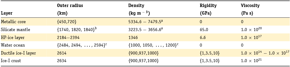
Since our research is focused on the tidal response of Ganymede in the presence of a subsurface ocean, our modelling of Ganymede's interior needs to take into account the previously discussed phase transitions within the water layer. As such, the basic structural models of Ganymede's interior in this paper will consist of five homogeneous layers: a metallic core, a rocky mantle, a HP-ice layer, a subsurface water ocean and an ice-I shell. The radius r and density ϱ of each of these layers need to be such that the entire model satisfies the constraints on average density and normalised mean moment of inertia, as well as additional compositional constraints on the densities of the two innermost layers: (i) for the metallic core we assume that the density ranges between ρc = 5330 kg m−3 (density of Fe-FeS) and ρc = 7800 kg m−3 (density of Fe) (e.g. see Sohl et al., Reference Sohl, Spohn, Breuer and Nagel2002) and (ii) for the silicate mantle we assume values between ρm = 3222 kg m−3 and ρm = 3800 kg m−3, where the first value is consistent with the presence of modest amounts of hydrated materials (Bland et al., Reference Bland, Showman and Tobie2009; Vance et al., Reference Vance, Bouffard, Choukroun and Sotin2014) while the latter is consistent with low concentrations of iron in the rock as a result of the differentiation of the metallic core (e.g. see Anderson et al., Reference Anderson, Lau, Sjogren, Schubert and Moore1996; Vance et al., Reference Vance, Bouffard, Choukroun and Sotin2014). Through the use of these constraints plausible values for the radii of Ganymede's internal layers can be determined following the constant density approach for interior modelling outlined in Sohl et al. (Reference Sohl, Spohn, Breuer and Nagel2002), in which the densities of the three water–ice layers are also assumed to be known. Reference values for these densities are ρhp = 1346 kg m−3, ρw = 1100 kg m−3 and ρI = 937 kg m−3, for, respectively, the HP-ice layer, the subsurface ocean and the ice-I shell (e.g. see Sohl et al., Reference Sohl, Spohn, Breuer and Nagel2002; Vance et al., Reference Vance, Bouffard, Choukroun and Sotin2014). Furthermore, in order to analyse the effect of the density of the upper layers on the tidal response, we allow the density of Ganymede's ocean to vary between ρw = 1000 kg m−3 and ρw = 1200 kg m−3, which are plausible values depending on the salinity of the ocean (Vance et al., Reference Vance, Bouffard, Choukroun and Sotin2014). Similarly, for the density of the ice-I shell the range ρw = 900–1000 kg m−3 is assumed to take into account the possible effect of porosity and impurities.
In addition, each internal layer is characterised by rheological parameters that give a representation of the layer's response to internal and/or external excitations. In this paper we have chosen to adopt the linear Maxwell viscoelastic model to describe the rheological behaviour of internal solid layers, mainly due to its simplicity and the large uncertainty in the knowledge of the rheological properties of materials at conditions relevant for icy satellites. According to the definition of the Maxwell model, the rheology of each internal solid layer is fully described by only two macroscopic parameters, namely the rigidity μ and the viscosity η. The ratio of these two parameters, the so-called Maxwell time  ${\tau _{\rm M}} = \frac{\eta }{\mu }$, gives an indication of the timescale at which the material under deformation shows a transition from elastic to viscous behaviour. Hence, a Maxwell viscoelastic layer will behave as an elastic layer at timescales much smaller than the Maxwell time (i.e. for t ≪ τM), whereas it will behave as a fluid body at timescales much larger than the Maxwell time (i.e. for t ≫ τM). On the other hand, internal liquid layers, such as the core and the water ocean, are treated as inviscid fluids (i.e. rigidity and viscosity are by definition equal to zero).
Even under the assumption of a Maxwell rheology, the rheological parameters that characterise the internal layers of icy satellites are largely uncertain or even unknown, therefore here we consider all previously defined internal layers to be homogeneous in terms of their rheology. Nevertheless, an exception is made for the ice-I shell, which is subdivided into two layers of different viscosity, but equal rigidity (Wahr et al., Reference Wahr, Zuber, Smith and Lunine2006), in order to simulate the effect of an effectively elastic icy crust on top of a more ductile lower part of the shell. The introduction of a viscosity contrast within the ice-I shell is consistent with thermal models dealing with solid-state convection in ice-I shells (e.g. Kirk & Stevenson, Reference Kirk and Stevenson1987; Showman et al., Reference Showman, Stevenson and Malhotra1997; Barr & Pappalardo, Reference Barr and Pappalardo2005; Tobie et al., Reference Tobie, Mocquet and Sotin2005; McKinnon, Reference McKinnon2006; Bland et al., Reference Bland, Showman and Tobie2009; Hammond & Barr, Reference Hammond and Barr2014) and with numerical models dealing with the morphology of impact craters on the surface of icy satellites (e.g. Schenk, Reference Schenk2002; Senft & Stewart, Reference Senft and Stewart2011). However, it needs to be pointed out that thermal models have been mostly applied to the study of the formation of grooved terrain in Ganymede's surface, which is thought to be the result of a period of global surface expansion due to either satellite differentiation or partial melting of the ice-I shell when Ganymede entered a possible Laplace-like resonance with Europa and Io (e.g. Showman et al., Reference Showman, Stevenson and Malhotra1997; Bland et al., Reference Bland, Showman and Tobie2009; Hammond & Barr, Reference Hammond and Barr2014). As a result, the chosen subdivision of the ice shell into a nearly elastic top layer and a ductile lower layer at the bottom may be more representative for the conditions in Ganymede's past and thus may not be a good description of the current thermal state of Ganymede's ice-I shell (e.g. Barr & Pappalardo, Reference Barr and Pappalardo2005).
Since the properties of the upper layers of an icy satellite are expected to dominate the tidal response, most variations in the rheological parameters are introduced in the definition of the rigidity and viscosity of the layers that simulate the ice-I shell. The value of the rigidity of ice-I (μI) at planetary conditions is uncertain by about one order of magnitude, with values as low as ~0.3 GPa (Vaughan, Reference Vaughan1995; Schmeltz et al., Reference Schmeltz, Rignot and MacAyeal2002; Wahr et al., Reference Wahr, Zuber, Smith and Lunine2006) and as high as ~10 GPa (Moore & Schubert, Reference Moore and Schubert2000; Harada & Kurita, Reference Harada and Kurita2006) being suggested as appropriate for research on icy satellites. Nevertheless, in the vast majority of research cases, the reference value for the rigidity of ice-I is most likely between 2 GPa and 4 GPa, which is a range that includes the value μI ≈ 2 GPa obtained from laboratory experiments involving periodic loading (2.5−3 hours) of unfractured saline ice at − 30°C (Cole & Durell, Reference Cole and Durell1995) and the value μI ≈ 3.5 GPa obtained from laboratory experiments on several samples of natural and artificial ice (Gammon et al., Reference Gammon, Kiefte and Clouter1983; Helgerud et al., Reference Helgerud, Waite, Kirby and Nur2009). The latter will be used as the reference value for the rigidity of the ice-I shell in our modelling, as it has been widely used as a reference value in previous research on tidal problems involving icy satellites (e.g. Tobie et al., Reference Tobie, Mocquet and Sotin2005; Rappaport et al., Reference Rappaport, Iess, Wahr, Lunine, Armstrong, Asmar, Tortora, Di Benedetto and Racioppa2008; Wahr et al., Reference Wahr, Selvans, Mullen, Barr, Collins, Selvans and Pappalardo2009; Jara-Orué & Vermeersen, Reference Jara-Orué and Vermeersen2011; Beuthe, Reference Beuthe2013; Shoji et al., Reference Shoji, Hussmann, Kurita and Sohl2013; Van Hoolst et al., Reference Van Hoolst, Baland and Trinh2013).
The viscosities of the layers that constitute the ice-I shell are the less-known rheological parameters in the modelling of icy satellites. The upper part of the shell, which is assumed to be 20 km thick in our modelling (e.g. see Schenk, Reference Schenk2002), is considered to be cold enough to behave in an effectively elastic way (Moore & Schubert, Reference Moore and Schubert2003), and hence its viscosity is assumed to be 1.0 × 10²¹ Pa s (larger values are plausible but will not influence the results). The lower part of the shell is considered to be more ductile as a result of either the increase in temperature with depth (if the shell is in conductive equilibrium) or the presence of a nearly isothermal convective layer (stagnant-lid/sluggish-lid convection case). To take both possible scenarios into account, we allow the viscosity of the lower part of the shell (ηast) to range between 1.0 × 10¹⁴ Pa s (around the value for the viscosity at melting temperature) and 1.0 × 10¹⁷ Pa s (effectively elastic response). Since the onset of convection is uncertain (e.g. Barr & Pappalardo, Reference Barr and Pappalardo2005), the latter will be used as reference value for the viscosity of the lower part of the shell.
The rheological parameters of the remaining internal viscoelastic layers are also poorly constrained, as the exact composition of these layers remains unknown. Commonly used values for the rigidity of a HP-ice layer (μhp) usually range between 4.6 GPa (ice-III) and 7.5 GPa (ice-VI) (Sohl et al., Reference Sohl, Spohn, Breuer and Nagel2002), while the corresponding values for the rigidity of the silicate mantle (μm) may range between 40 GPa and 100 GPa (e.g. Moore & Schubert, Reference Moore and Schubert2000; Sohl et al., Reference Sohl, Spohn, Breuer and Nagel2002, Reference Sohl, Solomonidou, Wagner, Coustenis, Hussmann and Schulze-Makuch2014; Rappaport et al., Reference Rappaport, Iess, Wahr, Lunine, Armstrong, Asmar, Tortora, Di Benedetto and Racioppa2008). As reference values, we adopt μhp = 6.6 GPa for the HP-ice layer (Sohl et al., Reference Sohl, Solomonidou, Wagner, Coustenis, Hussmann and Schulze-Makuch2014) and μm = 65 GPa for the silicate mantle (Turcotte & Schubert, Reference Turcotte and Schubert2014). Furthermore, to preclude viscoelastic relaxation to take place in the deeper layers of Ganymede, we assume ηm = 1.0 × 10²⁰ Pa s for the viscosity of the silicate mantle and ηm = 1.0 × 10¹⁷ Pa s for the viscosity of the HP-ice layer.
As an overview of the discussion in this section we have listed the reference values for each interior parameter in Table 1 (reference model) as well as the explored range of values for the interior parameters in Table 2.
Table 1. Reference six-layered model of Ganymede's interior (see text for an explanation of the values)

Table 2. Range of values for the several geophysical parameters that characterise the internal structure of Ganymede's proposed six-layered models (see text for an explanation of the values)

a The density of the core and the mantle are such that the entire interior model satisfies the imposed conditions on average density and mean moment of inertia.
b The value r m = 1840 km is only used for cases in which the density of the ocean is assumed to be lower than the reference value.
c Values within the given range are equally spaced.
Tidal response
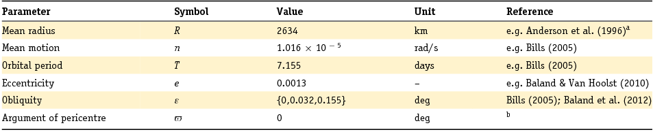
The tidal potential exerted by Jupiter on Ganymede experiences periodic variations on the timescale of the orbital motion – or diurnal timescale (period T ≈ 7.155 days, mean motion n = 1.016 × 10⁻⁵ rad/s) – as a result of Ganymede's slightly elliptical orbit (eccentricity e = 0.0013) and the likely non-zero, but small, obliquity of its spin axis (Bills, Reference Bills2005; Baland et al., Reference Baland, Yseboodt and Van Hoolst2012). Ganymede's eccentric orbit around Jupiter leads on one hand to stretching and squeezing of the tidal bulge, as a result of periodic changes in the Ganymede–Jupiter distance. On the other hand, Ganymede's instantaneous orbital motion is usually not equal to its spin rate as a result of its eccentric orbit, thereby leading to periodic longitudinal librations of the tidal bulge. Similarly, a non-zero obliquity leads to changes in the latitudinal orientation of the tidal bulge.
Using the method of Kaula (Reference Kaula1964), the diurnal tidal potential exerted by Jupiter at Ganymede's surface can be expressed in terms of the small eccentricity of Ganymede's orbit and the small obliquity of its spin axis by (Wahr et al., Reference Wahr, Selvans, Mullen, Barr, Collins, Selvans and Pappalardo2009; Jara-Orué & Vermeersen, Reference Jara-Orué and Vermeersen2011)
 $$\begin{eqnarray}
{\Phi _T} = {(nR)^2}\big\{ - \frac{{3e}}{2}P_{2,0}^\theta \cos (nt) + \frac{e}{4}P_{2,2}^\theta [3\cos \left( {2\phi } \right)\cos (nt) \nonumber\\
&& +\, 4\sin \left( {2\phi } \right)\sin (nt)] + P_{2,1}^\theta \sin (\varepsilon )\cos (\phi )\sin (\varpi + nt)\big\} \nonumber\\
\end{eqnarray}$$
$$\begin{eqnarray}
{\Phi _T} = {(nR)^2}\big\{ - \frac{{3e}}{2}P_{2,0}^\theta \cos (nt) + \frac{e}{4}P_{2,2}^\theta [3\cos \left( {2\phi } \right)\cos (nt) \nonumber\\
&& +\, 4\sin \left( {2\phi } \right)\sin (nt)] + P_{2,1}^\theta \sin (\varepsilon )\cos (\phi )\sin (\varpi + nt)\big\} \nonumber\\
\end{eqnarray}$$where all second- and higher-order terms in the small eccentricity and obliquity have been neglected. In Equation 1, R is the mean radius of Ganymede, ε is the obliquity of Ganymede's spin axis and ϖ is the argument of pericentre measured with respect to the ascending node where Ganymede's orbital plane crosses its equatorial plane. Values for these parameters are listed in Table 3. Moreover, the angles θ and ϕ are, respectively, the colatitude and the longitude of a point on Ganymede's surface. Finally, the associated Legendre polynomials P θ2, 0, P θ2, 1 and P θ2, 2 are defined by
 $$\begin{equation}
P_{2,0}^\theta = \frac{{3{{\cos }^2}(\theta ) - 1}}{2}
\end{equation}$$
$$\begin{equation}
P_{2,0}^\theta = \frac{{3{{\cos }^2}(\theta ) - 1}}{2}
\end{equation}$$ $$\begin{equation}
P_{2,1}^\theta = 3\sin (\theta )\cos (\theta )
\end{equation}$$
$$\begin{equation}
P_{2,1}^\theta = 3\sin (\theta )\cos (\theta )
\end{equation}$$ $$\begin{equation}
P_{2,2}^\theta = 3{\sin ^2}(\theta )
\end{equation}$$
$$\begin{equation}
P_{2,2}^\theta = 3{\sin ^2}(\theta )
\end{equation}$$Table 3. Radius, orbital parameters and rotational parameters of Ganymede
a The current value for Ganymede's mean radius is R = 2631.2 km (Archinal et al., Reference Archinal, A'hearn, Bowell, Conrad, Consolmagno, Courtin, Fukushima, Hestroffer, Hilton and Krasinsky2011). Although this value may lead to Love numbers slightly different than for R = 2634 km, the differences are small enough (less than 0.5%) that they will not affect the results and conclusions in this paper.
b Assumed value for modelling purposes.
Since Ganymede's interior is not rigid, the materials composing the interior of Ganymede will continuously deform in response to the acting diurnal tide ΦT. In geophysics, the response of a planetary body to forces like tides is usually expressed in terms of dimensionless numbers, the so-called tidal Love numbers h 2, l 2 and k 2 (Love, Reference Love1911), where h 2 and l 2 refer to the tidally driven radial and lateral deformation experienced by the interior and k 2 refers to the gravitational potential due to the tidally induced mass redistribution. Here, we make use of the analytical method outlined in Jara-Orué & Vermeersen (Reference Jara-Orué and Vermeersen2011) to determine the tidal Love numbers at the surface of several plausible geophysical models of Ganymede's interior. This method is largely based on the viscoelastic normal mode approach of Sabadini & Vermeersen (Reference Sabadini and Vermeersen2004), with some modifications in order to handle the presence of a subsurface ocean layer at shallow depth from the surface.
Since the JUICE mission is expected to measure Ganymede's surface displacements and variations of the gravitational potential due to diurnal tides (Grasset et al., Reference Grasset, Dougherty, Coustenis, Bunce, Erd, Titov, Blanc, Coates, Drossart, Fletcher, Hussmann, Jaumann, Krupp, Lebreton, Prieto-Ballesteros, Tortora, Tosi and Van Hoolst2013), our modelling in this paper will concentrate on the determination of the tidal Love numbers h 2 and k 2. Within the framework of the normal mode approach, these two Love numbers can be conveniently written as (Sabadini & Vermeersen, Reference Sabadini and Vermeersen2004; Jara-Orué & Vermeersen, Reference Jara-Orué and Vermeersen2011)
 $$\begin{equation}
{\tilde h_2}(s) = h_2^e + \sum\limits_{j = 1}^M {\frac{{h_2^j \cdot ( - {s_j})}}{{s - {s_j}}}}
\end{equation}$$
$$\begin{equation}
{\tilde h_2}(s) = h_2^e + \sum\limits_{j = 1}^M {\frac{{h_2^j \cdot ( - {s_j})}}{{s - {s_j}}}}
\end{equation}$$ $$\begin{equation}
{\tilde k_2}(s) = k_2^e + \sum\limits_{j = 1}^M {\frac{{k_2^j \cdot ( - {s_j})}}{{s - {s_j}}}}
\end{equation}$$
$$\begin{equation}
{\tilde k_2}(s) = k_2^e + \sum\limits_{j = 1}^M {\frac{{k_2^j \cdot ( - {s_j})}}{{s - {s_j}}}}
\end{equation}$$where he 2 and ke 2 are defined as the elastic Love numbers, the sj are the inverse relaxation times of the M relaxation modes of the interior, the hj 2 and kj 2 are the corresponding modal strengths, and s is the Laplace variable. The tilde on top of h 2 and k 2 indicates that the Love numbers are defined in the Laplace domain.
In the case of a periodic forcing, such as the diurnal tides, it is common to express the tidal Love numbers  ${\tilde h_2}$ and
  ${\tilde k_2}$ as functions of frequency (with s = iω in Equations 5 and 6). The resulting frequency-dependent Love numbers are complex, in which the real part denotes the part of the response in-phase with the forcing whereas the imaginary part refers to the part of the response out-of-phase with the forcing. This set of complex Love numbers are characterised by a magnitude
  $| {{{\tilde h}_2}(\omega )} | = {( {{\rm{Re}}{{({{\tilde h}_2}(\omega ))}^2} + {\rm{Im}}{{({{\tilde h}_2}(\omega ))}^2}} )^{0.5}}$ and a phase-lag
 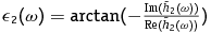 ${\epsilon _2}(\omega ) = \arctan ( { - \frac{{{\rm{Im}}({{\tilde h}_2}(\omega ))}}{{{\rm{Re}}({{\tilde h}_2}(\omega ))}}} )$.
Then, using the definition of the Love numbers (e.g. Love, Reference Love1911; Sabadini & Vermeersen, Reference Sabadini and Vermeersen2004), the actual radial deformation u r and perturbation potential ϕ1 experienced by Ganymede at its surface due to the acting diurnal tides can be expressed in the time domain as
 $$\begin{equation}
{u_{\rm{r}}}(t) = \frac{{{h_2}(t)}}{{{g_0}}} * {\Phi _{\rm{T}}}(t)
\end{equation}$$
$$\begin{equation}
{u_{\rm{r}}}(t) = \frac{{{h_2}(t)}}{{{g_0}}} * {\Phi _{\rm{T}}}(t)
\end{equation}$$ $$\begin{equation}- {\phi _1}(t) = {k_2}(t) * {\Phi _{\rm{T}}}(t)
\end{equation}$$
$$\begin{equation}- {\phi _1}(t) = {k_2}(t) * {\Phi _{\rm{T}}}(t)
\end{equation}$$where g 0 is the acceleration of gravity at Ganymede's surface (g 0 = 1.425 m s−2) and the symbol ∗ denotes time convolution. Explicit expressions for the tidal deformation u r and potential perturbation ϕ1 are commonly derived after transformation of Equations 7 and 8 to the Laplace domain (or alternatively to the Fourier domain) and subsequent substitution of Equations 5, 6 and the Laplace transform of Equation 1. After some analytical manipulation, the radial deformation u r at the surface may be written as
 $$\begin{equation}
{u_{\rm{r}}}(t) = u_{\rm{r}}^e(t) + u_{\rm{r}}^{\rm{v}}(t)
\end{equation}$$
$$\begin{equation}
{u_{\rm{r}}}(t) = u_{\rm{r}}^e(t) + u_{\rm{r}}^{\rm{v}}(t)
\end{equation}$$where the elastic component of the radial deformation (ue r) is defined by
 $$\begin{eqnarray}
u_{\rm{r}}^e(t) = \frac{1}{4}{(nR)^2}\frac{{h_2^e}}{{{g_0}}}( - 6eP_{2,0}^\theta \cos (nt) + eP_{2,2}^\theta [4\sin (2\phi )\sin (nt)\nonumber\\
&& + \, 3\cos (2\phi )\cos (nt)]\nonumber\\
&& + \, 4\sin (\varepsilon )P_{2,1}^\theta [\cos (\phi )\sin (\varpi + nt)])
\end{eqnarray}$$
$$\begin{eqnarray}
u_{\rm{r}}^e(t) = \frac{1}{4}{(nR)^2}\frac{{h_2^e}}{{{g_0}}}( - 6eP_{2,0}^\theta \cos (nt) + eP_{2,2}^\theta [4\sin (2\phi )\sin (nt)\nonumber\\
&& + \, 3\cos (2\phi )\cos (nt)]\nonumber\\
&& + \, 4\sin (\varepsilon )P_{2,1}^\theta [\cos (\phi )\sin (\varpi + nt)])
\end{eqnarray}$$and the deformation due to viscoelastic relaxation (u vr) is given by
 $$\begin{eqnarray}
u_{\rm{r}}^{\rm{v}}(t) = \frac{1}{4}{(nR)^2}\sum\limits_{j = 1}^M \bigg\{ \frac{{h_2^j}}{{{g_0}}}\frac{1}{{\sqrt {1 + \Gamma _j^2} }}( - 6eP_{2,0}^\theta \cos \left( {nt - \arctan ({\Gamma _j})} \right)\nonumber\\
&& +\, eP_{2,2}^\theta [4\sin (2\phi )\sin \left( {nt - \arctan ({\Gamma _j})} \right) \nonumber\\
&& +\, 3\cos (2\phi )\cos \left( {nt - \arctan ({\Gamma _j})} \right)]\nonumber\\
&& +\, 4\sin (\varepsilon )P_{2,1}^\theta [\cos (\phi )\sin \left( {\varpi + nt - \arctan ({\Gamma _j})} \right)])\bigg\}
\end{eqnarray}$$
$$\begin{eqnarray}
u_{\rm{r}}^{\rm{v}}(t) = \frac{1}{4}{(nR)^2}\sum\limits_{j = 1}^M \bigg\{ \frac{{h_2^j}}{{{g_0}}}\frac{1}{{\sqrt {1 + \Gamma _j^2} }}( - 6eP_{2,0}^\theta \cos \left( {nt - \arctan ({\Gamma _j})} \right)\nonumber\\
&& +\, eP_{2,2}^\theta [4\sin (2\phi )\sin \left( {nt - \arctan ({\Gamma _j})} \right) \nonumber\\
&& +\, 3\cos (2\phi )\cos \left( {nt - \arctan ({\Gamma _j})} \right)]\nonumber\\
&& +\, 4\sin (\varepsilon )P_{2,1}^\theta [\cos (\phi )\sin \left( {\varpi + nt - \arctan ({\Gamma _j})} \right)])\bigg\}
\end{eqnarray}$$An important parameter in the definition of the contribution of an individual relaxation mode j to the experienced tidal deformation is the ratio Γj, which is defined as the ratio between the mean angular velocity of Ganymede's orbit (n) and the inverse relaxation time ( − sj) of the jth relaxation mode, i.e.
 $$\begin{equation}
{\Gamma _j} = \frac{n}{{ - {s_j}}} = \frac{{2\pi {\tau _j}}}{T}
\end{equation}$$
$$\begin{equation}
{\Gamma _j} = \frac{n}{{ - {s_j}}} = \frac{{2\pi {\tau _j}}}{T}
\end{equation}$$where τj is the relaxation time of the normal mode j. Similar expressions can be derived for the potential perturbation.
As can be seen from Equation 11, the dimensionless ratio Γj has two important effects on the contribution of a relaxation mode j to the radial deformation at the surface: (i) it attenuates the magnitude of the modal strength hj 2 and (ii) it causes a phase-lag in the corresponding response. As discussed in Jara-Orué & Vermeersen (Reference Jara-Orué and Vermeersen2011) for the case of the viscoelastic response of jovian moon Europa, most relaxation modes have relaxation times that are several orders of magnitude larger than the orbital period and hence their contribution to the radial deformation may be considered to be negligibly small. However, some of the so-called transient modes (e.g. see Sabadini & Vermeersen (Reference Sabadini and Vermeersen2004) for their definition) may have relaxation times that are sufficiently short to have a theoretical contribution to the experienced radial deformation at the surface. Transient modes are generally weak, with the notable exception of the ones due to the viscosity contrast introduced within the ice-I shell, therefore the non-elastic part of Ganymede's tidal response is expected to be dominated by the rheological properties of the lower part of the ice-I shell, similarly to the case of Europa (Jara-Orué & Vermeersen, Reference Jara-Orué and Vermeersen2011).
Results
Application of the normal mode approach to a diverse range of plausible interior models of Ganymede allows us to study how the tidal response at the surface depends on the geophysical parameters that characterise its internal structure. As a first step, several interior models of Ganymede are constructed using the range of values presented in Table 2, thereby taking into consideration that all generated models should satisfy the constraints introduced earlier. As can be observed in Table 2, most of the variations are introduced in the parameters that characterise the upper layers, as these layers are expected to have a dominant influence on the tidal response at the surface (e.g. see Moore & Schubert, Reference Moore and Schubert2003).
As a next step, we determine the frequency-dependent complex tidal Love numbers  ${\tilde h_2}$ and
  ${\tilde k_2}$ by applying the methodology described earlier to the generated interior models of Ganymede. Since the normal mode model is inherently viscoelastic, the non-elastic part of the response includes the contribution of nine normal modes: the core mode C 0, the buoyancy modes M 0 and M 1 at the ocean-HP-ice boundary and HP-ice-mantle boundary, respectively, the L 0 buoyancy mode at the ocean-ice-I boundary, the surface mode S 0, the transient modes TM 1 and TM 2 at the boundary between the HP-ice mantle and the silicate mantle, and the transient modes TS 1 and TS 2 at the introduced viscosity contrast within the ice-I shell (e.g. Sabadini & Vermeersen, Reference Sabadini and Vermeersen2004). Although many of these relaxation modes are strong enough to influence the properties of the tidal response at lower frequencies (ω ≪ n), only the fastest and strongest of the transient modes at the introduced viscosity contrast within the ice-I shell (here
  ${\textit TS}_{1}$) may have a non-negligible contribution to the tidal response at the high frequency of the acting diurnal tides. To illustrate this statement, we first express the contribution of the
  ${\textit TS}_{1}$ mode to, for example, the tidal Love number
  ${\tilde h_2}$ at the frequency of the acting forcing (ω = n) in terms of the ratio ω = n through the use of Equations 5 and 12, i.e.
 $$\begin{equation}
\frac{{h_2^j \cdot ( - {s_j})}}{{in - {s_j}}} = \frac{{h_2^j}}{{1 + \Gamma _j^2}} - i\frac{{h_2^j{\Gamma _j}}}{{1 + \Gamma _j^2}}
\end{equation}$$
$$\begin{equation}
\frac{{h_2^j \cdot ( - {s_j})}}{{in - {s_j}}} = \frac{{h_2^j}}{{1 + \Gamma _j^2}} - i\frac{{h_2^j{\Gamma _j}}}{{1 + \Gamma _j^2}}
\end{equation}$$
for  $j = {\textit TS}_{1}$.
If the viscosity of the ductile ice layer is too small, such that the inverse relaxation time of the strong transient mode  ${\textit TS}_{1}$ is much larger than the orbital frequency (i.e. − sj ≫ n or Γj ≪ 1, viscous relaxation in the lower part of the ice-I shell takes place rapidly and hence the layer will show a fluid-like behaviour at the forcing frequency. This behaviour can be deduced from Equation 13, as the imaginary part goes to zero for Γj ≪ 1 whereas the real part approaches the fluid behaviour he 2 + h 2j. On the other hand, if the viscosity in the lower part of the ice-I shell is too large (i.e. for − sj ≪ n or Γj ≫ 1, viscous relaxation does not take place in the lower part of the ice-I shell and hence the response of the layer will be effectively elastic. In this case, both the real and imaginary parts of the contribution of the transient mode
  ${\textit TS}_{1}$ approach zero and therefore the tidal response is effectively dominated by the elastic response. A different behaviour takes place when the viscosity of the lower part of the ice-I shell is such (e.g. ηast = 5.0 × 10¹⁴ Pa s) that a strong transient mode with inverse relaxation time − sj ≈ n (i.e. Γj ≈ 1) is present in the tidal response. In this scenario viscoelastic relaxation within the lower part of the ice-I shell would lead to an increase in the magnitude of the deformation compared to the effectively elastic case (non-negligible real part in Equation 13) and would introduce a phase-lag of some degrees in the tidal response (non-negligible imaginary part in Equation 13).
A more concrete analysis of the dependence of the tidal response at the surface on the parameters that characterise Ganymede's ice-I shell can be obtained from the curves shown in Figs 1 and 2, where the magnitude of the complex Love numbers h 2 and k 2 at frequency ω = n is depicted as a function of the ice-I shell thickness for a range of plausible values for the rigidity and viscosity of the shell. We clearly observe in Figs 1 and 2 that the magnitude of the Love numbers decreases nearly linearly with increasing thickness of the ice-I shell, with the rate of decrease being strongest for effectively elastic shells with a large value for the rigidity (~35% for h 2 and ~37% for k 2 in the thickness range 40–150 km). In addition, we observe that larger values for the rigidity of ice-I (μI) lead in all depicted cases to smaller values for the Love numbers, with the effect being largest for effectively elastic shells as well.
Fig. 1. Radial deformation tidal Love number h2 as a function of the thickness of the ice-I shell for models with ice-I rigidities µI = 1 GPa, µI = 3.5 GPa (reference models) and µI = 10 GPa. The curves are shown for two different values for the viscosity of the ductile part of ice-I layer: (1) for a low viscosity at which viscoelastic relaxation affects the diurnal response to the acting tides and (2) for a high viscosity at which the diurnal response is effectively elastic.
Fig. 2. Gravitational perturbation tidal Love number k2 as a function of the thickness of the ice-I shell for models with ice-I rigidities µI = 1 GPa, µI = 3.5 GPa (reference models) and µI = 10 GPa. The curves are shown for two different values for the viscosity of the ductile part of ice-I layer: (1) for a low viscosity at which viscoelastic relaxation affects the diurnal response to the acting tides and (2) for a high viscosity at which the diurnal response is effectively elastic.
Furthermore, as shown by the dash-dotted curves in Figs 1 and 2, lowering the viscosity of the ductile part of the shell from ηast = 1.0 × 10¹⁷ Pa s to ηast = 1.0 × 10¹⁴ Pa s would reduce the sensitivity that the magnitude of the Love numbers has on variations in the thickness and rigidity of the ice-I shell. As expected, the changes in the magnitude of the Love numbers as a result of the lower viscosity are largest for thick and very rigid shells, with changes up to ~37% for both h 2 and k 2 within the given viscosity range.
Although the densities of Ganymede's upper layers are not as poorly constrained as the thickness and rheological parameters of the ice-I shell, uncertainty in their values may also lead to non-negligible effects on the magnitude of the Love numbers h 2 and k 2. In particular, the effect of the density of the ocean may be large and nearly comparable in magnitude to the effect of the thickness and/or rigidity of the ice-I shell, especially for the Love number k 2. As can be deduced from the curves shown in Fig. 3, the magnitude of both Love numbers decreases with decreasing density of the ocean by as much as 6% for h 2 and 23% for k 2 within the explored range of ocean densities (1000–1200 kg m3). The sensitivity of the amplitude of the Love numbers on the density of the ice-I shell is smaller. As shown in Fig. 4, the amplitude of both Love numbers decreases with decreasing ice-I density by at most ~ 3% for h 2 and ~ 4.5% for k 2 within the explored range of values for the density of the ice-I shell (900–1000 kg m3).
Fig. 3. Tidal Love numbers h2 and k2 as a function of the thickness of the ice-I shell for models with ocean density ρw = 1000 kg m−3, ρw = 1050 kg m−3, ρw = 1100 kg m−3 (reference models), ρw = 1150 kg m−3 and ρw = 1200 kg m−3. The upper cluster of curves refers to the radial deformation tidal Love number h2, whereas the lower cluster (dash-dotted curves) refers to the Love number k2. In all cases the density of the ice-I shell is taken at ρI = 937 kg m−3 and the rigidity at µI = 3.5 GPa.
Fig. 4. Tidal Love numbers h2 and k2 as a function of the thickness of the ice-I shell for models with ice-I density ρI = 900 kg m−3, ρI = 937 kg m−3 (reference models) and ρI = 1000 kg m−3. The upper cluster of curves refers to the radial deformation tidal Love number h2, whereas the lower cluster (dash-dotted curves) refers to the Love number k2. In all cases the density of the ocean is taken at ρI = 1100 kg m−3 and the rigidity of the ice-I shell at µI = 3.5 GPa.
Other parameters that characterise the internal structure of Ganymede have a much smaller effect on the magnitude of the tidal Love numbers at the surface. For example, the sensitivity of the Love numbers on the size of the HP-ice layer is so small that it cannot be noticed from Figs 1–4 that the depicted curves are obtained by combining the tidal response of models with different values for the size of the HP-ice layer. In a similar way, the size and density of the deepest internal layers have a negligible effect on the magnitude of the tidal Love numbers (e.g. less than 0.1% for h 2 and around 0.2% for k 2 if a smaller core is used for the modelling). The rheological parameters of the silicate mantle and HP-ice layer may have a larger effect on the tidal Love numbers if the layers are soft, as the inverse relaxation times of their corresponding normal modes M 1 and M 0 will shift towards the orbital frequency, thereby increasing the amplitude and phase-lag of the Love numbers.
So far, we have shown our results in terms of the Love numbers which give a representation of the tidal response experienced by Ganymede. The actual tidal deformation is obtained from substitution of the calculated Love numbers into Equations 9–11. For our reference interior model of Ganymede (see Table 1), the maximum radial displacement at the surface due to the acting diurnal tides during one orbital revolution is displayed in Fig. 5A for the case in which the obliquity is assumed to be equal to zero. The shown (single) amplitude of the largest surface displacements ( ~ 3 m) is slightly lower than in previous research, mainly due to our choice for the geophysical parameters that characterise the reference model. However, our results are within the uncertainty range in those models and their values ( ~ 4 m) could be replicated by choosing a thinner shell, a less rigid shell or a less viscous ductile part of the shell.
Fig. 5. Maximum radial displacement (single amplitude) at the surface of Ganymede due to the acting diurnal tides. A. Obliquity ε = 0°; B. Obliquity ε = 0.032°; C. Obliquity ε = 0.155°. In all cases, the interior of Ganymede is described by our reference model and Table 1 and the argument of pericenter ϖ is assumed to be equal to 0°.
In contrast to, for example, Europa or Titan, even small obliquities – such as the ones proposed in the study by Baland et al. (Reference Baland, Yseboodt and Van Hoolst2012) – can have a noticeable effect on the tidal deformation patterns at the surface (see Fig. 5B). The relatively large effect of the contribution of Ganymede's small obliquity to the deformation is mainly a consequence of the small eccentricity of its orbit relative to the assumed value for the obliquity (e.g. compare the relative difference between e = 0.0013 and sin(ε) = 0.00059 for ε = 0.032° in the case of Ganymede with e = 0.0094 and sin(ε) = 0.00077 for ε = 0.044° in the case of Europa, with both values for the obliquity being taken from Baland et al. (Reference Baland, Yseboodt and Van Hoolst2012)). As a result, larger values for the unknown obliquity, such as the ε = 0.155° proposed by Bills (Reference Bills2005), will lead to a large contribution to the surface displacement due to the acting diurnal tides. Then, as shown in Fig. 5C, the obliquity tide will start to dominate the deformation patterns at the surface and the amplitude of the deformation will increase with respect to the eccentricity-only case. Although not shown here, changing the value of the unknown argument of pericenter ϖ will also lead to different deformation patterns at the surface.
On the other hand, the contribution of forced longitudinal librations (not shown here) will remain small, as the libration amplitude is usually much smaller ( ~ 10−6 (Van Hoolst et al., Reference Van Hoolst, Baland and Trinh2013)) than the one from the optical libration (2e) that is part of the eccentricity tide.
Discussion and conclusions
In this paper we have presented a normal mode-based method to determine the time-dependent tidal Love numbers h 2 and k 2 at the surface of a viscoelastic Ganymede in the case that a subsurface ocean is assumed to be present in the interior. If the tidal response of Ganymede's interior at the diurnal frequency is considered to be effectively elastic, i.e. no relaxation in the ice-I shell, the amplitude of the radial displacement Love number h 2 is mostly sensitive to the uncertainties in the thickness and rigidity of the ice-I shell, as can be observed from Fig. 1. In addition, Fig. 3 shows that the Love number h 2 is also sensitive to the poorly constrained density of the ocean, with its contribution being more important in the lower – and most plausible – range of values for the rigidity of the shell (i.e. μI = [1, 3.5] GPa), and for thinner shells. Other internal parameters have a small effect on its amplitude, with the density of the ice-I shell having the largest effect by introducing an uncertainty of a few percent.
The sensitivity of the gravitational perturbation Love number k 2 on the parameters that characterise the interior is a bit different. As for h 2, the Love number k 2 is mostly sensitive to the thickness and rigidity of the shell, but also to a larger extent to the density of the ocean (see Figs 2 and 3 for the preferred range of rigidities μI = [1, 3.5] GPa). The large dependence of k 2 on the density of the ocean is in agreement with the results obtained by, for example, Baland et al. (Reference Baland, Tobie, Lefèvre and Van Hoolst2014) for the case of Titan, which aimed to provide a possible explanation for the large value of k 2 (k 2 = 0.589 ± 0.150 and k 2 = 0.637 ± 0.224) obtained from observations of the acceleration of the Cassini spacecraft during six flybys (Iess et al., Reference Iess, Jacobson, Ducci, Stevenson, Lunine, Armstrong, Asmar, Racioppa, Rappaport and Tortora2012). In the hypothetical case that such values would apply to the case of Ganymede as well, the results shown in Figs 2 and 3 would indicate that the Love number implies the presence of a dense ocean in combination with a preferably thin and not very rigid ice-I shell.
The introduction of a low-viscosity ductile ice-I layer adds one extra poorly constrained parameter to our analysis, i.e. the viscosity of the ductile part of the shell. As shown in Figs 1 and 2, the sensitivity of the Love numbers h 2 and k 2 on the large uncertainties in the viscosity of this layer is comparable to their sensitivity on the also poorly constrained rigidity. This effect is expected as lowering the viscosity leads to a reduction in the effective rigidity of a layer (e.g. see Equation 50 in Jara-Orué & Vermeersen (Reference Jara-Orué and Vermeersen2011)). In addition, the introduction of a low-viscosity layer may lead to a phase-lag in the tidal response, which can be a few degrees if the ratio Γj (see Equation 12) of the dominating transient mode  ${\textit TS}_{1}$ of the viscoelastic response is in the range Γj = [0.1, 10]. Note, however, that the discussion presented here on the effect of viscoelasticity on the tidal response of Ganymede is based on our description of the rheology by use of the simple Maxwell model. Hence, the numerical results representing the sensitivity of the Love numbers on the rheology only apply to a Maxwell rheology and may be different if more complex – and perhaps more realistic – anelastic rheologies (Burgers, Andrade) are used in the modelling (e.g. see McCarthy & Castillo-Rogez (Reference McCarthy and Castillo-Rogez2013) for a discussion about rheological models for ice-I relevant to icy satellites).
Since the accuracy of measurements of the tidal Love number k 2 of Ganymede by the 3GM instrument is expected to be around 10−3 for both the real and imaginary parts (Parisi et al., Reference Parisi, Iess and Finocchiaro2014), the determination of k 2 would provide an unambiguous assessment about the presence or absence of a subsurface ocean in Ganymede's interior (recall that k 2 for oceanless models is expected to be smaller than 0.2 (Moore & Schubert, Reference Moore and Schubert2003) for ice-I viscosities larger than the reference viscosity at the melting temperature ( ~ 1013 Pa s), while our models always predict values larger than 0.3 in the presence of a subsurface ocean). The characterisation of the geophysical properties of the shell and the ocean is, however, substantially more challenging as many configurations may be representative for the same Love number. For example, an assumed value of k 2 = 0.48 could fit any shell thickness in the range ~40–130 km (derived from Fig. 3) due to uncertainties in the ocean density, even if the rigidity of ice-I would be known to be equal to the reference value of 3.5 GPa. Measurements of the tidal Love number h 2 and the quantity Δ = 1 + k 2 − h 2 (Wahr et al., Reference Wahr, Zuber, Smith and Lunine2006) may have the potential, if sufficiently accurate, to narrow down the possible range of values for the thickness of Ganymede's shell as h 2 is less sensitive to the uncertainties in the ocean density (see Fig. 3). In addition, uncertainties due to the unknown rigidity of ice-I can be narrowed down by measurements of the amplitude of the longitudinal librations of the shell by GALA and/or imaging of the surface, as the shell librations are expected to be very sensitive to the rigidity of ice-I (Van Hoolst et al., Reference Van Hoolst, Baland and Trinh2013; Jara-Orué & Vermeersen, Reference Jara-Orué and Vermeersen2014).
Acknowledgments
Part of this research has been financially supported by the GO program of the Netherlands Organization for Scientific Research (NWO). We thank two anonymous reviewers for their comments on an earlier version of this manuscript.