


1. Introduction and motivation
Wearable sensors are being increasingly used in medicine to monitor important physiological parameters. Patients with type I diabetes, for example, wear a sensor inserted under the skin which provides measurements of the interstitial blood glucose level (BGL) every 5 minutes. Sensor bands provide a non-invasive solution to measuring additional physiological parameters, such as temperature, skin conductivity, heart rate, and acceleration of body movements. Patients may also self-report information about discrete life events such as meals, sleep, or stressful events, while an insulin pump automatically records two types of insulin interventions: a continuous stream of insulin called the basal rate, and discrete self-administered insulin dosages called boluses. The data acquired from sensors and patients accumulate rapidly and lead to a substantial data overload for the health provider.
To help doctors more easily browse the wealth of generated patient data, we developed PhysioGraph, a graphical user interface (GUI) that displays various time series of measurements acquired from a patient. As shown in Figure 1, PhysioGraph displays the data corresponding to one day, whereas buttons allow the user to move to the next or previous day. Clicking on any measurement or event displays additional data, such as amount of carbohydrates for a meal or the amount of insulin for a bolus event. The user also has the option of toggling off the display of specific time series, in order to reduce clutter.

Figure 1. PhysioGraph window displaying one day’s worth of patient data (default view). The blue graph at the top shows the entire timeline of blood glucose measurements, over approximately 8 weeks. The top pane below it shows physiological parameters, including heart rate (red) and skin conductivity (green). The bottom pane shows time series of blood glucose (blue), basal insulin (black), and estimated active insulin (red). Discrete life events such as meals and exercise are shown at the top of the bottom pane, whereas boluses are shown at the bottom. When an event is clicked, details are displayed in the pane on the right.
While PhysioGraph was enthusiastically received by doctors, it soon became apparent that the doctor–GUI interaction could be improved substantially if the tool also allowed for natural language (NL) interactions. Most information needs are highly contextual and local. For example, if the blood glucose spiked after a meal, the doctor would often want to know more details about the meal or about the bolus that preceded the meal. The doctors often found it easier to express their queries in NL, for example, “show me how much he ate,” “did he bolus before that,” resulting in a sub-optimal situation where the doctor would ask this type of local questions in English while a member of our team would perform the clicks required to answer the question, for example, click on the meal event, to show details such as amount of carbohydrates. Furthermore, there were also global questions, such as “how often does the patient go low in the morning and the evening,” whose answers required browsing the entire patient history in the worst case, which was very inefficient. This motivated us to work on a new question answering (QA) paradigm that allows users to express their information needs using NL queries and direct actions within a GUI. To this end, we propose a pipeline architecture comprised of two major modules: first, a speech recognizer transcribes the doctor’s spoken question into text; then the text is converted by a semantic parser into a logical form (LF). The LF can be run by an inference engine to automatically retrieve the answer from the database storing the patient data. The new QA paradigm described in this paper has the potential for applications in many areas of medicine where sensor data and life events are pervasive. The proposed intelligent user interface will also benefit the exploration and interpretation of data in other domains such as experimental physics, where large amounts of time series data are generated from high-throughput experiments.
The structure of the paper is as follows: Section 2 describes the new QA setting and its major distinguishing features; Section 3 details the speech recognition module and its evaluation; Section 4 focuses on the semantic parsing system and its performance when using correct textual input; Section 5 presents an empirical evaluation of the entire semantic parsing pipeline. The paper ends with related work and concluding remarks.
2. Task definition and distinguishing features
Figure 2 shows an example of interaction with PhysioGraph, where the doctor first clicks on a hypoglycemia event, represented by the red triangle in the bottom pane. To determine what kind of food the patient ate in response to the hypoglycemia event, the doctor then asks the question “ What did she eat for her snack?”. The question is first transcribed into text by the speech recognition module. The transcribed question is then used as input to the semantic parsing system, which produces its formal representation, that is, its LF $Answer(e.food) \wedge e.type=Meal \wedge Around(e.time, e(-1).time)$
. Note that the patient had multiple meals (shown as blue squares) on the particular day shown in PhysioGraph. To determine the correct meal intended by the doctor, the semantic parsing module takes into account the fact that the doctor previously clicked on the hypoglycemia event. This serves as an anchoring action and therefore the correct meal should be the one that is close to the hypoglycemia event, as reflected by the clause
$Answer(e.food) \wedge e.type=Meal \wedge Around(e.time, e(-1).time)$
. Note that the patient had multiple meals (shown as blue squares) on the particular day shown in PhysioGraph. To determine the correct meal intended by the doctor, the semantic parsing module takes into account the fact that the doctor previously clicked on the hypoglycemia event. This serves as an anchoring action and therefore the correct meal should be the one that is close to the hypoglycemia event, as reflected by the clause $Around(e.time, e(-1).time)$
in the LF. In this example, the context dependency is realized by referencing the focus event of the previous interaction, formally represented as
$Around(e.time, e(-1).time)$
in the LF. In this example, the context dependency is realized by referencing the focus event of the previous interaction, formally represented as $e(-1).time$
. Once the LF is generated, an answer retrieval engine can easily return the answer by performing a query against the back-end database.
$e(-1).time$
. Once the LF is generated, an answer retrieval engine can easily return the answer by performing a query against the back-end database.

Figure 2. The proposed semantic parsing pipeline for context-dependent question answering.
Table 1. Examples of interactions and logical forms
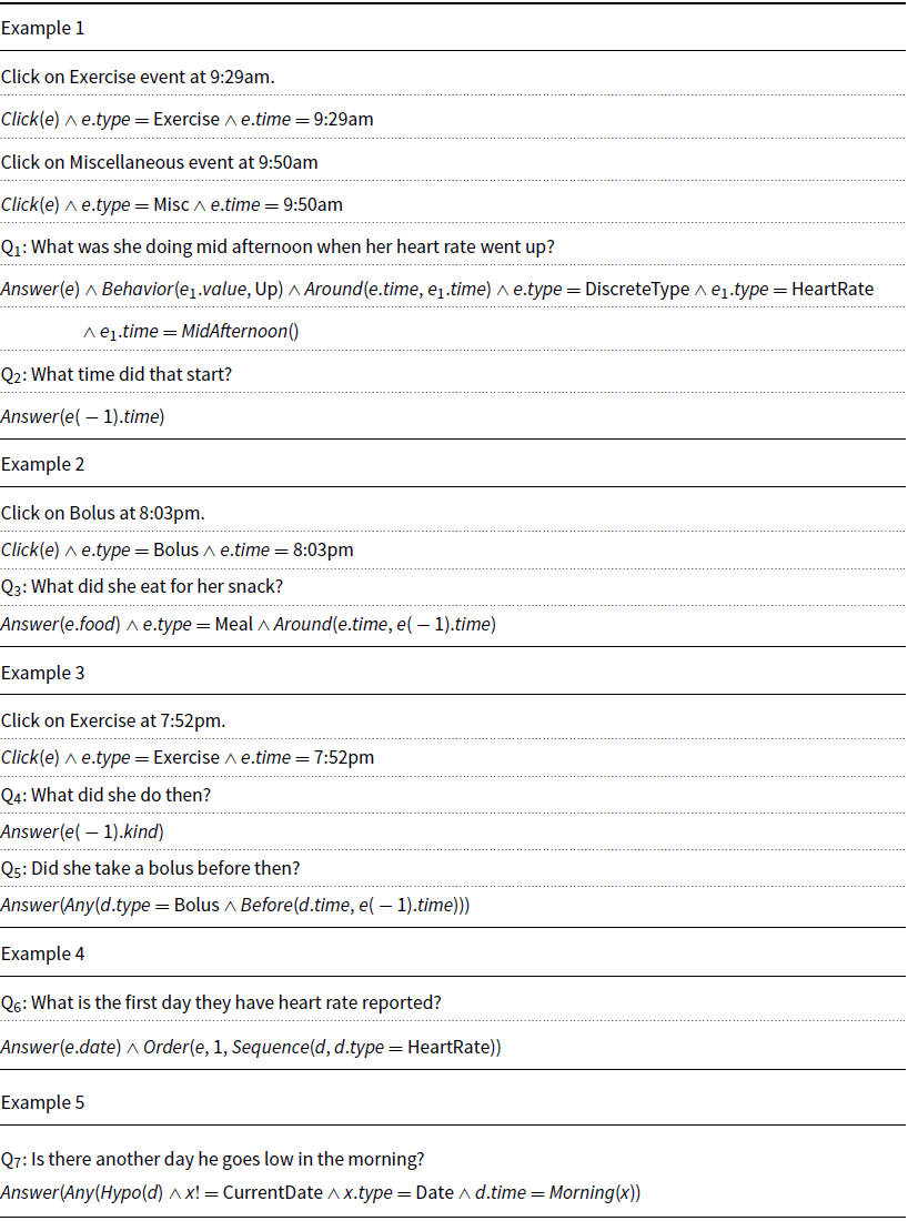
Table 1 shows additional sample inputs paired with their LFs. For each input, the examples also show relevant previous inputs from the interaction sequence. The LFs often contain constants, such as dates or specific times during the day, which are out of the LF vocabulary. When translating NL queries, these out-of-vocabulary (OOV) constants will be copied from the NL input into the LF using a copy mechanism, as will be described in Section 4.3. A separate copying mechanism will also be used for referencing events in the previous LF.
In the following, we describe a number of major features that, on their own or through their combination, distinguish the proposed QA paradigm from other QA tasks powered by semantic parsing.
2.1 Time is essential
All events and measurements in the knowledge base are organized in time series. Consequently, many queries contain time expressions, such as the relative “midnight” or the coreferential “then,” and temporal relations between relevant entities, expressed through words such as “after” or “when.” This makes processing of temporal relations essential for good performance. Furthermore, the GUI serves to anchor the system in time, as most of the information needs expressed in local questions are relative to the day shown in the GUI, or the last event that was clicked.
2.2 GUI interactions versus NL questions
The user can interact with the system (1) directly within the GUI (e.g. mouse clicks); (2) through NL questions; or (3) through a combination of both, as shown in Examples 1 and 2 in Table 1. Although the result of every direct interaction with the GUI can also be obtained using NL questions, sometimes it can be more convenient to use the GUI directly, especially when all events of interest are in the same area of the screen and thus easy to move the mouse or hand from one to the other. For example, a doctor interested in what the patient ate that day can simply click on the blue squares shown at the bottom pane in PhysioGraph, one after another. Sometimes a click can be used to anchor the system at a particular time during the day, after which the doctor can ask short questions implicitly focused on that region in time. An example of such hybrid behavior is shown in Example 2, where a click on a Bolus event is followed by a question about a snack, which implicitly should be the meal right after the bolus.
2.3 Factual queries versus GUI commands
Most of the time, doctors have information needs that can be satisfied by clicking on an event shown in the GUI or by asking factual questions about a particular event of interest from that day. In contrast, a different kind of interaction happens when the doctor wants to change what is shown in the tool, such as toggling on/off particular time series, for example, “toggle on heart rate,” or navigating to a different day, for example, “go to next day,” “look at the previous day.” Sometimes, a question may be a combination of both, as in “what is the first day they have a meal without a bolus?”, for which the expectation is that the system navigates to that day and also clicks on the meal event to show additional information and anchor the system at the time of that meal.
2.4 Sequential dependencies
The user interacts with the system through a sequence of questions or clicks. The LF of a question, and implicitly its answer, may depend on the previous interaction with the system. Examples 1–3 in Table 1 are all of this kind. In example 1, the pronoun “that” in question 2 refers to the answer to question 1. In example 2, the snack refers to the meal around the time of the bolus event that was clicked previously – this is important, as there may be multiple snacks that day. In example 3, the adverb “then” in question 5 refers to the time of the event that is the answer of the previous question. As can be seen from these examples, sequential dependencies can be expressed as coreference between events from different questions. Coreference may also occur within questions, as in question 4 for example. Overall, solving coreferential relations will be essential for good performance.
3. Speech recognition
This section describes the speech recognition system, which is the first module in the proposed semantic parsing pipeline. Given a spoken question or command coming from the user, the task is to transcribe it automatically into text. For this, we adapt the neural end-to-end model proposed by Zeyer et al. (Reference Zeyer, Irie, Schlüter and Ney2018), a publicly available open source system that was trained on LibriSpeech and which at the time of its publication obtained state-of-the-art results, that is, a word error rate (WER) of 3.82% on the test-clean subset of LibriSpeech. While this represents a competitive performance on in-domain data, its WER on the speech recorded from the two doctors in our study was much higher, and thus insufficiently accurate for the semantic parsing module downstream. For lack of free access to a better speech recognizer, our solution was to fine-tune the LibriSpeech-trained model of Zeyer et al. (Reference Zeyer, Irie, Schlüter and Ney2018) on a small parallel corpus obtained from each doctor, taking advantage of the fact that the encoder–decoder architecture used by this system is relatively simple and straightforward to retrain or fine-tune. First, each input audio file is converted into a Mel-frequency cepstral coefficients (MFCC) representation (Sigurdsson, Petersen, and Lehn-Schiøler Reference Sigurdsson, Petersen and Lehn-Schiøler2006). The encoder consists of six layers of bi-directional long short-term memories (LSTMs) that project the MFCC vectors into a sequence of latent representations which are then used to initialize the decoder, a one-layer bi-directional LSTM. The decoder operates on subword-level units, such as characters and graphemes, which are created through byte-pair encoding (BPE) (Sennrich, Haddow, and Birch Reference Sennrich, Haddow and Birch2016). An individual grapheme may or may not carry meaning by itself, and may or may not correspond to a single phoneme of the spoken language. The advantage for using subword-level units as output is that it allows recognition of unseen words and does not require a large softmax output which is computationally expensive. Therefore, during training, the manually transcribed text is first processed via BPE to create subword units, which are then used as the actual output targets of the decoder. At each step, the decoder computes attention weights over the sequence of hidden states produced by the encoder and uses them to calculate a corresponding context vector. Together with the current state in the decoder, the context vector is used as input to the softmax that generates the BPE unit for the current step. Once the decoding is complete, all the generated BPE units are merged into a sequence of words. Stochastic gradient descent with global gradient clipping is utilized to train the entire encoder-attention-decoder architecture.
3.1 Experimental evaluation
The speech from two doctorsFootnote 1 was recorded while they were using PhysioGraph, resulting in two datasets, Amber and Frank. The corresponding transcripts of the speech, including queries and commands, are obtained by manual annotation. The end-to-end speech recognition model (Zeyer et al. Reference Zeyer, Irie, Schlüter and Ney2018), which was originally trained on LibriSpeech, is fine-tuned separately for each of the two datasets. In order to improve the recognition performance, in a second set of experiments, we also apply data augmentation. A more detailed description of the evaluation procedure follows.
The speech recognition system was first trained and tested on the Amber dataset using a 10-fold evaluation scenario where the dataset is partitioned into 10 equal size folds, and each fold is used as test data while the remaining 9 folds are used for training. WER is used as the evaluation metric, and the final performance is computed as the average WER over the 10 folds. We denote this system as SR.Amber (Amber without data augmentation). In addition, we evaluate the speech recognition system with data augmentation. The system in this evaluation scenario is denoted as SR.Amber + Frank, which means that Amber is the target data, while Frank is the external data used for data augmentation. We use the same 10 folds of data used in the SR.Amber evaluation, where for each of the 10 folds used as test data, all examples in the Frank dataset are added to the remaining 9 folds of the Amber dataset that are used for training. The final performance of SR.Amber + Frank is computed as the average WER over the 10 folds.
The WER performance of the speech recognition system on the Amber dataset, with and without data augmentation, is shown in the top half of Table 2. The experimental results indicate that SR.Amber + Frank outperforms SR.Amber, which means that data augmentation is able to improve the performance in this evaluation scenario. In order to further investigate the impact of data augmentation, we run a similar evaluation setup on the Frank dataset, using the Amber dataset for augmentation. The corresponding results for SR.Frank and SR.Frank + Amber are shown in the bottom half of Table 2. Here, too, data augmentation is shown to be beneficial. The improvement of SR.Frank + Amber over SR.Frank and SR.Amber + Frank over SR.Amber is both statistically significant at $p = 0.02$
in a one-tailed paired t-test.
$p = 0.02$
in a one-tailed paired t-test.
Table 2. Performance of speech recognition system on dataset Amber and dataset Frank with and without data augmentation. SR.Amber and SR.Frank are two systems without data augmentation while SR.Amber + Frank and SR.Frank + Amber are two systems enhanced with data augmentation. WER (%) is the evaluation metric

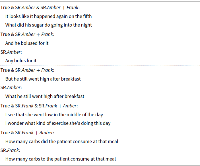
Table 3 reports outputs from the speech recognition system, demonstrating that data augmentation is able to correct some of the mistakes made by the baseline systems.
Table 3. Examples of transcriptions generated by SR systems trained on SR.Frank and SR.Amber, and their augmented versions SR.Frank + Amber and SR.Amber + Frank, respectively. True refers to the correct transcription
4. Context-dependent semantic parsing
The role of the semantic parsing module is to take the text version of the doctor’s queries and commands and convert it into a formal representation, that is, the LF. We first introduce the evaluation datasets in Section 4.1, followed by a description of the neural network architectures in Sections 4.2 and 4.3, and the experimental evaluation in Section 4.4.
4.1 Semantic parsing datasets
To train and evaluate semantic parsing approaches, we created three datasets of sequential interactions: two datasets of real interactions (Section 4.1.1) and a much larger dataset of artificial interactions (Section 4.1.2).
4.1.1 Real interactions
We recorded interactions with the GUI in real time, using data from 9 patients, each with around 8 weeks worth of time series data. The interactions were acquired from two physicians, Frank Schwartz, MD and Amber Healy, DO, and were stored in two separate datasets called Frank and Amber, respectively. In each recording session, the tool was loaded with data from one patient and the physician was instructed to explore the data in order to understand the patient behavior as usual, by asking NL questions or interacting directly with the GUI. Whenever a question was asked, a member of our study team found the answer by navigating in PhysioGraph and clicking on the corresponding events. After each session, the question segments were extracted manually from the speech recordings, transcribed, and timestamped. The transcribed speech was used to fine-tune the speech recognition models, as described in Section 3. All direct interactions (e.g. mouse clicks) were recorded automatically by the tool, timestamped, and exported into an XML file. The sorted list of questions and the sorted list of mouse clicks were then merged using the timestamps as key, resulting in a chronologically sorted list of questions and GUI interactions. Mouse clicks were automatically translated into LFs, whereas questions were parsed into LFs manually, to be used for training and evaluating the semantic parsing algorithms. Sample interactions and their LFs are shown in Table 1.
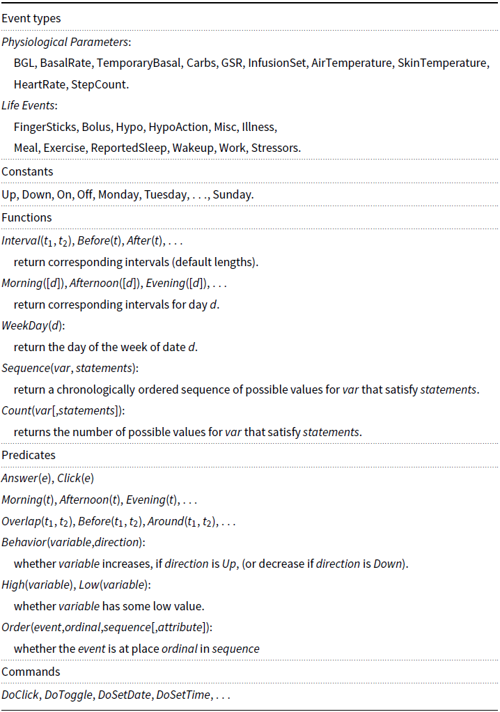
A snapshot of the vocabulary for LFs is shown in Table 4, detailing the Event Types, Constants, Functions, Predicates, and Commands. Every life event or physiological measurement stored in the database is represented in the LFs as an event object e with 3 major attributes: $e.type$
,
$e.type$
, $e.date$
, and
$e.date$
, and $e.time$
. Depending on its type, an event object may contain additional fields. For example, if
$e.time$
. Depending on its type, an event object may contain additional fields. For example, if $e.type = BGL$
, then it has an attribute
$e.type = BGL$
, then it has an attribute $e.value$
. If
$e.value$
. If $e.type = Meal$
, then it has attributes
$e.type = Meal$
, then it has attributes $e.food$
and
$e.food$
and $e.carbs$
. We use
$e.carbs$
. We use $e(-i)$
to represent the event appearing in the
$e(-i)$
to represent the event appearing in the $i{\rm th}$
previous LF. Thus, to reference the event mentioned in the previous LF, we use
$i{\rm th}$
previous LF. Thus, to reference the event mentioned in the previous LF, we use $e(-1)$
, as shown for question Q
$e(-1)$
, as shown for question Q $_5$
. If more than one event appears in the previous LF, we use an additional index j to match the event index in the previous LF. Coreference between events is represented simply using the equality operator, for example,
$_5$
. If more than one event appears in the previous LF, we use an additional index j to match the event index in the previous LF. Coreference between events is represented simply using the equality operator, for example, $e = e(-1)$
.
$e = e(-1)$
.
Table 4. Vocabulary for logical forms
Overall, the LFs in the two datasets have the following statistics:
-
• The Frank dataset contains LFs for 237 interactions, corresponding to 74 mouse clicks and 163 NL queries.
-
‐ The LFs for 43 NL queries reference an event from the previous LF.
-
‐ The LFs for 26 NL queries contain OOV tokens that can be copied from the NL input.
-
• The Amber dataset contains LFs for 504 interactions, corresponding to 330 mouse clicks and 174 NL queries.
-
‐ The LFs for 97 NL queries reference an event from the previous LF.
-
‐ The LFs for 35 NL queries contain OOV tokens that can be copied from the NL input.
4.1.2 Artificial interactions
The number of annotated real interactions is too small for training an effective semantic parsing model. To increase the number of training examples, we developed an artificial data generator, previously described in Chen et al. (Reference Chen, Mirshekarian, Bunescu and Marling2019). To simulate user–GUI interactions, the artificial data generator uses sentence templates in order to maintain high-quality sentence structure and grammar. This approach is similar to Weston et al. (Reference Weston, Bordes, Chopra and Mikolov2016), with the difference that we need a much higher degree of variation such that the machine learning model does not memorize all possible sentences, which resulted in a much richer template database. The template language is defined using a recursive grammar, which allows creating as many templates and generating as many data examples as desired. We used the same vocabulary as for the real interactions dataset. To generate contextual dependencies (e.g. event coreference), the implementation allows for more complex combo templates where a sequence of templates are instantiated together. A more detailed description of the template language and the simulator implementation is given in Chen et al. (Reference Chen, Mirshekarian, Bunescu and Marling2019) and Appendix A, together with illustrative examples. The simulator was used to generate 1000 interactions and their LFs: 312 mouse clicks and 688 NL queries.
4.2 Baseline models for semantic parsing
In this section, we describe two baseline models: a standard LSTM encoder–decoder for sequence generation SeqGen and its attention-augmented version SeqGen+Att2In. The attention-based model will be used later in Section 4.3 as a component in the context-dependent semantic parsing architecture.
As shown in Figure 3, the sequence generation model SeqGen uses LSTM (Hochreiter and Schmidhuber Reference Hochreiter and Schmidhuber1997) units in an encoder–decoder architecture (Cho et al. Reference Cho, van Merriënboer, Gülçehre, Bahdanau, Bougares, Schwenk and Bengio2014; Bahdanau, Cho, and Bengio Reference Bahdanau, Cho, Bengio, Bengio and LeCun2015), composed of a bi-directional LSTM for the encoder and a unidirectional LSTM for the decoder. The Bi-LSTM encoder is run over the input sequence X in both directions and the two final states (one from each direction) are concatenated to produce the initial state $\textbf{s}_0$
for the decoder. Starting from the initial hidden state
$\textbf{s}_0$
for the decoder. Starting from the initial hidden state $\textbf{s}_0$
, the decoder produces a sequence of states
$\textbf{s}_0$
, the decoder produces a sequence of states $\textbf{s}_1,\ldots,\textbf{s}_m$
. Both the encoder and the decoder use a learned embedding function e for their input tokens. We use
$\textbf{s}_1,\ldots,\textbf{s}_m$
. Both the encoder and the decoder use a learned embedding function e for their input tokens. We use $X =x_1, \ldots, x_n$
to represent the sequence of tokens in the NL input, and
$X =x_1, \ldots, x_n$
to represent the sequence of tokens in the NL input, and $Y = y_1, \ldots, y_m$
to represent the tokens in the corresponding LF. We use
$Y = y_1, \ldots, y_m$
to represent the tokens in the corresponding LF. We use $Y_t = y_1, \ldots, y_t$
to denote the LF tokens up to position t, and
$Y_t = y_1, \ldots, y_t$
to denote the LF tokens up to position t, and $\hat{Y}$
to denote the entire LF generated by the decoder. A softmax is used by the decoder to compute token probabilities at each position as follows:
$\hat{Y}$
to denote the entire LF generated by the decoder. A softmax is used by the decoder to compute token probabilities at each position as follows:
 \begin{align} p(y_t|Y_{t-1}, X) & = softmax(\textbf{W}_h \textbf{s}_{t}) \end{align}
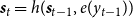
 \begin{align} \textbf{s}_t & = h(\textbf{s}_{t - 1}, e(y_{t-1})) \nonumber\end{align}
The transition function h is implemented by the LSTM unit (Hochreiter and Schmidhuber Reference Hochreiter and Schmidhuber1997).

Figure 3. The SeqGen model takes a sequence of natural language (NL) tokens as input $X =x_1, \ldots, x_n$
and encodes it with a Bi-LSTM (left, green). The two final states are used to initialize the decoder LSTM (right, blue) which generates the LF sequence
$X =x_1, \ldots, x_n$
and encodes it with a Bi-LSTM (left, green). The two final states are used to initialize the decoder LSTM (right, blue) which generates the LF sequence $\hat{Y} = \hat{y}_1, \ldots, \hat{y}_m$
. The attention-augmented SeqGen+Att2In model computes attention weights (blue arrows) and a context vector (red arrow) for each position in the decoder.
$\hat{Y} = \hat{y}_1, \ldots, \hat{y}_m$
. The attention-augmented SeqGen+Att2In model computes attention weights (blue arrows) and a context vector (red arrow) for each position in the decoder.
Additionally, the SeqGen+Att2In model uses an attention mechanism Att2In to compute attention weights and a context vector $\textbf{c}_t$
for each position in the decoder, as follows:
$\textbf{c}_t$
for each position in the decoder, as follows:
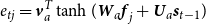
 \begin{align}e_{tj} & = \textbf{v}_{a}^T \tanh(\textbf{W}_{a} \textbf{f}_{j} + \textbf{U}_{a} \textbf{s}_{t-1}) \end{align}
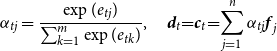
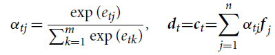 \begin{align}\alpha_{tj} & = \frac{\exp(e_{tj})}{\sum_{k=1}^{m}\exp(e_{tk})} \nonumber, \:\:\:\:\:\textbf{d}_t\!=\!\textbf{c}_t\!=\!\sum_{j=1}^{n}\alpha_{tj}\textbf{f}_j \nonumber\end{align}
We follow the attention mechanism formulation of Bahdanau et al. (Reference Bahdanau, Cho, Bengio, Bengio and LeCun2015) where, at each time step t in the decoder, the softmax output depends not only on the current LSTM state $\textbf{s}_t$
but also an an additional context vector
$\textbf{s}_t$
but also an an additional context vector $\textbf{c}_t$
that aims to capture relevant information from the input sequence. The context vector is formulated as a weighted combination of the hidden states
$\textbf{c}_t$
that aims to capture relevant information from the input sequence. The context vector is formulated as a weighted combination of the hidden states $\textbf{f}_j$
computed by the Bi-LSTM encoder over the input NL sequence, using a vector of attention weights
$\textbf{f}_j$
computed by the Bi-LSTM encoder over the input NL sequence, using a vector of attention weights $\alpha_{tj}$
, one attention weight for each position j in the input sequence. The attention vector is obtained by applying softmax to a vector of unnormalized weights
$\alpha_{tj}$
, one attention weight for each position j in the input sequence. The attention vector is obtained by applying softmax to a vector of unnormalized weights $e_{tj}$
computed from the hidden state
$e_{tj}$
computed from the hidden state $\textbf{f}_j$
in the encoder and the previous decoder state
$\textbf{f}_j$
in the encoder and the previous decoder state $\textbf{s}_{t - 1}$
. The context vector
$\textbf{s}_{t - 1}$
. The context vector $\textbf{d}_t = \textbf{c}_t$
and the current decoder state
$\textbf{d}_t = \textbf{c}_t$
and the current decoder state $\textbf{s}_t$
are then used as inputs to a softmax that computes the distribution for the next token
$\textbf{s}_t$
are then used as inputs to a softmax that computes the distribution for the next token $\hat{y}_t$
in the LF:
$\hat{y}_t$
in the LF:
 \begin{align} \hat{y}_t & \sim \text{softmax}(\textbf{W}_h \textbf{s}_t + \textbf{W}_d \textbf{d}_t) \end{align}
4.3 Semantic parsing with multiple levels of attention and copying mechanism
Figure 4 shows the proposed context-dependent semantic parsing model, SP+Att2All+Copy (SPAAC). Similar to the baseline models, we use a bi-directional LSTM to encode the input and another LSTM as the decoder. Context dependency is modeled using two types of mechanisms: attention and copying. The attention mechanism is composed of three models: Att2HisIn attending to the previous input, Att2HisLF attending to the previous LF, and the Att2In introduced in Section 4.2 that attends to the current input. The copying mechanism is composed of two models: one for handling unseen tokens and one for handling coreference to events in the current and previous LFs.
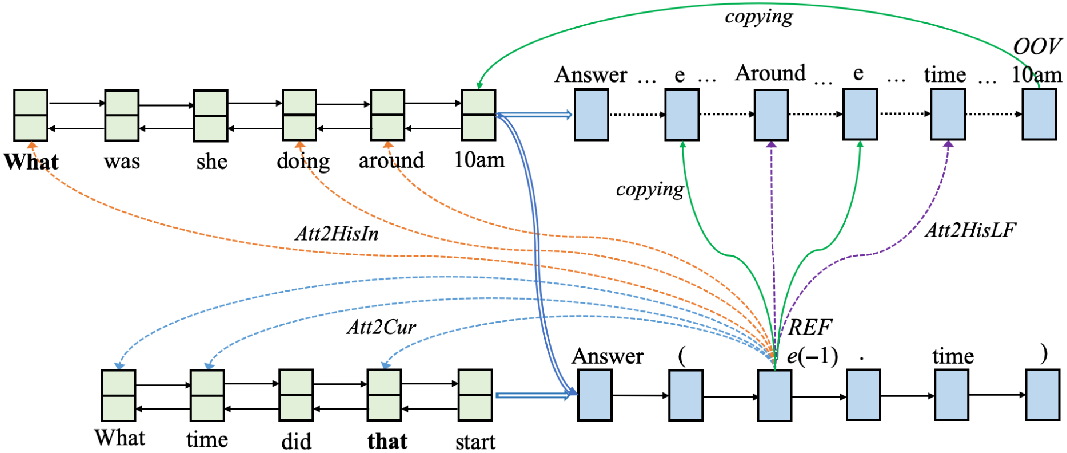
Figure 4. Context-dependent semantic parsing architecture. We use a Bi-LSTM (left) to encode the input and a LSTM (right) as the decoder. Top shows the previous interaction and bottom shows the current interaction. The complete previous LF is $Y^{-1}$
= [Answer, (, e,),
$Y^{-1}$
= [Answer, (, e,), $\wedge$
, Around, (, e,., time, OOV,),
$\wedge$
, Around, (, e,., time, OOV,), $\wedge$
, e,., type, =, DiscreteType]. The token 10am is copied from the input to replace the generated OOV token (green arrow). The complete current LF is Y = [Answer, (, REF,., time,)]. The entity token e(-1) is copied from the previous LF to replace the generated REF token (green arrow). To avoid clutter, only a subset of the attention lines (dotted) are shown.
$\wedge$
, e,., type, =, DiscreteType]. The token 10am is copied from the input to replace the generated OOV token (green arrow). The complete current LF is Y = [Answer, (, REF,., time,)]. The entity token e(-1) is copied from the previous LF to replace the generated REF token (green arrow). To avoid clutter, only a subset of the attention lines (dotted) are shown.
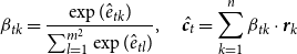
Attention Mechanisms At decoding step t, the Att2HisIn attention model computes the context vector $\hat{\textbf{c}_t}$
as follows:
$\hat{\textbf{c}_t}$
as follows:
 \begin{align}\hat{e}_{tk} & = \textbf{v}_b^T \tanh(\textbf{W}_b \textbf{r}_{k} + \textbf{U}_b \textbf{s}_{t-1}) \end{align}
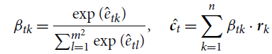 \begin{align}\beta_{tk} & = \frac{\exp(\hat{e}_{tk})}{\sum_{l=1}^{m^2}\exp(\hat{e}_{tl})} \nonumber,\:\:\:\:\:\hat{\textbf{c}_t} = \sum_{k=1}^{n}\beta_{tk} \cdot \textbf{r}_k \nonumber\end{align}
where $\textbf{r}_k$
is the encoder hidden state corresponding to
$\textbf{r}_k$
is the encoder hidden state corresponding to $\textbf{x}_k$
in the previous input
$\textbf{x}_k$
in the previous input $X^{-1}$
,
$X^{-1}$
, $\hat{\textbf{c}_t}$
is the context vector, and
$\hat{\textbf{c}_t}$
is the context vector, and $\beta_{tk}$
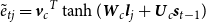
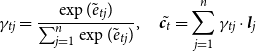
is an attention weight. Similarly, the Att2HisLF model computes the context vector
$\beta_{tk}$
is an attention weight. Similarly, the Att2HisLF model computes the context vector $\tilde{\textbf{c}_t}$
as follows:
$\tilde{\textbf{c}_t}$
as follows:
 \begin{align}\tilde{e}_{tj} & = {\textbf{v}_c}^T \tanh(\textbf{W}_c \textbf{l}_{j} + \textbf{U}_c \textbf{s}_{t-1}) \end{align}
 \begin{align}\gamma_{tj} & = \frac{\exp(\tilde{e}_{tj})}{\sum_{j=1}^{n}\exp(\tilde{e}_{tj})} \nonumber,\:\:\:\:\:\tilde{\textbf{c}_t} = \sum_{j=1}^{n}\gamma_{tj} \cdot \textbf{l}_j \nonumber\end{align}
where $\textbf{l}_j$
is the j-th hidden state of the decoder for the previous LF
$\textbf{l}_j$
is the j-th hidden state of the decoder for the previous LF $Y^{-1}$
.
$Y^{-1}$
.
The context vector $\textbf{d}_t$
is comprised of the context vectors from the three attention models Att2In, Att2HisIn, and Att2HisLF, and will be used in the decoder softmax as shown previously in Equation (3):
$\textbf{d}_t$
is comprised of the context vectors from the three attention models Att2In, Att2HisIn, and Att2HisLF, and will be used in the decoder softmax as shown previously in Equation (3):
 \begin{align}\textbf{d}_t = concat(\textbf{c}_t, \hat{\textbf{c}_t}, \tilde{\textbf{c}_t})\end{align}
Copying Mechanisms In order to handle OOV tokens and coreference (REF) between entities in the current and the previous LFs, we add two special tokens OOV and REF to the LF vocabulary. Inspired by the copying mechanism in Gu et al. (Reference Gu, Lu, Li and Li2016), we train the model to learn which token in the current input $X=\{x_j\}$
is an OOV by minimizing the following loss:
$X=\{x_j\}$
is an OOV by minimizing the following loss:
 \begin{align}L_{oov}(Y) & = -\sum_{j=1}^{X.l} \sum_{t=1}^{Y.l} \log p_o(O_{jt} | \textbf{s}^{X}_{j}, \textbf{s}^{Y}_{t})\end{align}
where $X.l$
is the length of current input,
$X.l$
is the length of current input, $Y.l$
is the length of the current LF,
$Y.l$
is the length of the current LF, $\textbf{s}^{X}_{j}$
is the LSTM state for
$\textbf{s}^{X}_{j}$
is the LSTM state for $x_j$
, and
$x_j$
, and $\textbf{s}^{Y}_{t}$
is the LSTM state for
$\textbf{s}^{Y}_{t}$
is the LSTM state for $y_t$
.
$y_t$
. $O_{jt} \in \{0, 1\}$
is a label that is 1 iff
$O_{jt} \in \{0, 1\}$
is a label that is 1 iff $x_{j}$
is an OOV and
$x_{j}$
is an OOV and $y_{t}=x_{j}$
. We use logistic regression to compute the OOV probability, that is,
$y_{t}=x_{j}$
. We use logistic regression to compute the OOV probability, that is, $p_o(O_{jt} = 1 | \textbf{s}^{X}_{j}, \textbf{s}^{Y}_{t}) = \sigma(\textbf{W}^{T}_{o}[\textbf{s}^{X}_{j},\textbf{s}^{Y}_{t}])$
.
$p_o(O_{jt} = 1 | \textbf{s}^{X}_{j}, \textbf{s}^{Y}_{t}) = \sigma(\textbf{W}^{T}_{o}[\textbf{s}^{X}_{j},\textbf{s}^{Y}_{t}])$
.
Similarly, to solve coreference, the model is trained to learn which entity in the previously generated LF $\hat{Y}^{-1}=\{\hat{y}_j\}$
is coreferent with the entity in the current LF by minimizing the following loss:
$\hat{Y}^{-1}=\{\hat{y}_j\}$
is coreferent with the entity in the current LF by minimizing the following loss:
 \begin{align}L_{ref}(Y) & = -\sum_{j=1}^{\hat{Y}^{-1}.l} \sum_{t=1}^{Y.l} \log p_r(R_{jt} | \textbf{s}^{\hat{Y}^{-1}}_{j}\!\!, \textbf{s}^{Y}_{t})\end{align}
where $\hat{Y}^{-1}.l$
is the length of the previous generated LF,
$\hat{Y}^{-1}.l$
is the length of the previous generated LF, $Y.l$
is the length of the current LF,
$Y.l$
is the length of the current LF, $\textbf{s}^{\hat{Y}^{-1}}_{j}$
is the LSTM state at position j in
$\textbf{s}^{\hat{Y}^{-1}}_{j}$
is the LSTM state at position j in $\hat{Y}^{-1}$
, and
$\hat{Y}^{-1}$
, and $\textbf{s}^{Y}_{t}$
is the LSTM state for position t in Y.
$\textbf{s}^{Y}_{t}$
is the LSTM state for position t in Y. $R_{jt} \in \{0, 1\}$
is a label that is 1 iff
$R_{jt} \in \{0, 1\}$
is a label that is 1 iff $\hat{y}_{j}$
is an entity referred by
$\hat{y}_{j}$
is an entity referred by $y_t$
in the next LF Y. We use logistic regression to compute the coreference probability, that is,
$y_t$
in the next LF Y. We use logistic regression to compute the coreference probability, that is, $p_r(R_{jt} = 1 | \textbf{s}^{\hat{Y}^{-1}}_{j}, \textbf{s}^{Y}_{t}) = \sigma(\textbf{W}^{T}_{r}[\textbf{s}^{\hat{Y}^{-1}}_{j}, \textbf{s}^{Y}_{t}])$
.
$p_r(R_{jt} = 1 | \textbf{s}^{\hat{Y}^{-1}}_{j}, \textbf{s}^{Y}_{t}) = \sigma(\textbf{W}^{T}_{r}[\textbf{s}^{\hat{Y}^{-1}}_{j}, \textbf{s}^{Y}_{t}])$
.
4.3.1 Token-level supervised learning: SPAAC-MLE
We use teacher forcing (Williams and Zipser Reference Williams and Zipser1989) to train the three models to learn which token in the vocabulary (including special tokens OOV and REF) should be generated. Correspondingly, the two baselines will minimize the following token generation loss:
 \begin{align}L_{gen}(Y) = -\sum_{t=1}^{{Y}.l} \log p(y_t | {Y}_{t-1}, X)\end{align}
where ${Y}.l$
is the length of the current LF. The supervised learning model SPAAC-MLE is obtained by training the semantic parsing architecture from Figure 4 to minimize the sum of the three negative log-likelihood losses:
${Y}.l$
is the length of the current LF. The supervised learning model SPAAC-MLE is obtained by training the semantic parsing architecture from Figure 4 to minimize the sum of the three negative log-likelihood losses:
 \begin{align}L_{MLE}(Y)\!=\! L_{gen}(Y)\! +\! L_{oov}(Y)\! + \!L_{ref}(Y)\end{align}
At inference time, the decoder is run in auto-regressive mode, which means that the input at step t is the previously generated token $\hat{y}_{t-1}$
. To alleviate the suboptimality of this greedy procedure, beam search is used to generate the LF sequence (Ranzato et al. Reference Ranzato, Chopra, Auli and Zaremba2016; Wiseman and Rush Reference Wiseman and Rush2016). During inference, if the generated token at position t is OOV, the token from the current input X that has the maximum OOV probability is copied, that is,
$\hat{y}_{t-1}$
. To alleviate the suboptimality of this greedy procedure, beam search is used to generate the LF sequence (Ranzato et al. Reference Ranzato, Chopra, Auli and Zaremba2016; Wiseman and Rush Reference Wiseman and Rush2016). During inference, if the generated token at position t is OOV, the token from the current input X that has the maximum OOV probability is copied, that is, $\mathop{\rm arg\,max}_{1\leq j\leq X.l} p_o(O_j = 1 | \textbf{s}^{X}_{j}, \textbf{s}^{Y}_{t})$
. Similarly, if the generated entity token at position t is REF, the entity token from the previously generated LF sequence
$\mathop{\rm arg\,max}_{1\leq j\leq X.l} p_o(O_j = 1 | \textbf{s}^{X}_{j}, \textbf{s}^{Y}_{t})$
. Similarly, if the generated entity token at position t is REF, the entity token from the previously generated LF sequence $\hat{Y}^{-1}$
that has the maximum coreference probability is copied, that is,
$\hat{Y}^{-1}$
that has the maximum coreference probability is copied, that is, $\mathop{\rm arg\,max}_{1 \leq j \leq Y^{-1}.l} p_r(R_j = 1 | \textbf{s}^{\hat{Y}^{-1}}_{j}, \textbf{s}^{\hat{Y}}_t)$
.
$\mathop{\rm arg\,max}_{1 \leq j \leq Y^{-1}.l} p_r(R_j = 1 | \textbf{s}^{\hat{Y}^{-1}}_{j}, \textbf{s}^{\hat{Y}}_t)$
.
4.3.2 Sequence-level reinforcement learning: SPAAC-RL
All models described in this paper are evaluated using sequence-level accuracy, a discrete metric where a generated LF is considered to be correct if it is equivalent with the ground truth LF. This is a strict evaluation measure in the sense that it is sufficient for a token to be wrong to invalidate the entire sequence. At the same time, there can be multiple generated sequences that are correct, for example, any reordering of the clauses from the ground truth sequence is correct. The large number of potentially correct generations can lead MLE-trained models to have sub-optimal performance (Zeng et al. Reference Zeng, Luo, Fidler and Urtasun2016; Norouzi et al. Reference Norouzi, Bengio, Jaitly, Schuster, Wu and Schuurmans2016; Rennie et al. Reference Rennie, Marcheret, Mroueh, Ross and Goel2017; Paulus, Xiong, and Socher Reference Paulus, Xiong and Socher2018). Furthermore, although teacher forcing is widely used for training sequence generation models, it leads to exposure bias (Ranzato et al. Reference Ranzato, Chopra, Auli and Zaremba2016): the network has knowledge of the ground truth LF tokens up to the current token during training, but not during testing, which can lead to propagation of errors at generation time.
Like Paulus et al. (Reference Paulus, Xiong and Socher2018), we address these problems using policy gradient to train a token generation policy that aims to directly maximize sequence-level accuracy. We use the self-critical policy gradient training algorithm proposed by Rennie et al. (Reference Rennie, Marcheret, Mroueh, Ross and Goel2017). We model the sequence generation process as a sequence of actions taken according to a policy, which takes an action (token $\hat{y}_t$
) at each step t as a function of the current state (history
$\hat{y}_t$
) at each step t as a function of the current state (history $\hat{Y}_{t-1}$
), according to the probability
$\hat{Y}_{t-1}$
), according to the probability $p(\hat{y}_t | \hat{Y}_{t-1})$
. The algorithm uses this probability to define two policies: a greedy, baseline policy
$p(\hat{y}_t | \hat{Y}_{t-1})$
. The algorithm uses this probability to define two policies: a greedy, baseline policy $\pi^b$
that takes the action with the largest probability, that is,
$\pi^b$
that takes the action with the largest probability, that is, $\pi^b(\hat{Y}_{t-1}) = \mathop{\rm arg\,max}_{\hat{y}_t} p(\hat{y}_t | \hat{Y}_{t-1})$
; and a sampling policy
$\pi^b(\hat{Y}_{t-1}) = \mathop{\rm arg\,max}_{\hat{y}_t} p(\hat{y}_t | \hat{Y}_{t-1})$
; and a sampling policy $\pi^s$
that samples the action according to the same distribution, that is,
$\pi^s$
that samples the action according to the same distribution, that is, $\pi^s(\hat{Y}_{t-1}) \propto p(\hat{y}_t | \hat{Y}_{t-1})$
.
$\pi^s(\hat{Y}_{t-1}) \propto p(\hat{y}_t | \hat{Y}_{t-1})$
.
The baseline policy is used to generate a sequence $\hat{Y}^b$
, whereas the sampling policy is used to generate another sequence
$\hat{Y}^b$
, whereas the sampling policy is used to generate another sequence $\hat{Y}^s$
. The reward
$\hat{Y}^s$
. The reward $R(\hat{Y}^s)$
is then defined as the difference between the sequence-level accuracy (A) of the sampled sequence
$R(\hat{Y}^s)$
is then defined as the difference between the sequence-level accuracy (A) of the sampled sequence $\hat{Y}^s$
and the baseline sequence
$\hat{Y}^s$
and the baseline sequence $\hat{Y}^b$
. The corresponding self-critical policy gradient loss is
$\hat{Y}^b$
. The corresponding self-critical policy gradient loss is
 \begin{align}L_{RL} = - R(\hat{Y}^s) \times L_{MLE}(\hat{Y}^s) = -\! \left(\!A(\hat{Y}^s)\! -\! A(\hat{Y}^b)\!\right) \times L_{MLE}(\hat{Y}^s)\end{align}
Thus, minimizing the RL loss is equivalent to maximizing the likelihood of the sampled $\hat{Y}^s$
if it obtains a higher sequence-level accuracy than the baseline
$\hat{Y}^s$
if it obtains a higher sequence-level accuracy than the baseline $\hat{Y}^b$
.
$\hat{Y}^b$
.
4.4 Experimental evaluation
All models are implemented in Tensorflow using dropout to alleviate overfitting. The feed-forward neural networks dropout rate was set to 0.5 and the LSTM units dropout rate was set to 0.3. The word embeddings and the LSTM hidden states had dimensionality of 64 and were initialized at random. Optimization is performed with the Adam algorithm (Kingma and Ba Reference Kingma and Ba2015), using an initial learning rate of 0.0001 and a minibatch size of 128. All experiments are performed on a single NVIDIA GTX1080 GPU.
Table 5. Sequence-level accuracy on the Artificial dataset and the two Real interactions datasets
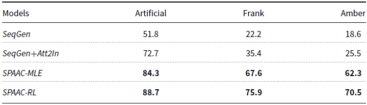
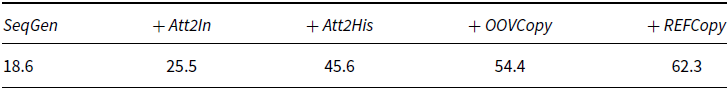
Table 6. Ablation results on the Amber dataset, as we gradually add more components to SeqGen
For each dataset, we use 10-fold evaluation, where the data are partitioned into 10 folds, one fold is used for testing and the remaining for training. The process is repeated 10 times to obtain test results on all folds. The embeddings for both the input vocabulary and output vocabulary are initialized at random and trained together with the other model parameters. Preliminary experiments did not show a significant benefit from using pre-trained input embeddings, likely due to the limited vocabulary. To model tokens that have not been seen at training time, we train a special $<$
unknown
$<$
unknown $>$
embedding by assigning it to tokens that appear only once during training. Subword embeddings may provide a better approach to dealing with unknown input words at test time, especially when coupled with contextualized embeddings provided by transformer-based models such as BERT (Devlin et al. Reference Devlin, Chang, Lee and Toutanova2019). We leave these enhancements for future work.
$>$
embedding by assigning it to tokens that appear only once during training. Subword embeddings may provide a better approach to dealing with unknown input words at test time, especially when coupled with contextualized embeddings provided by transformer-based models such as BERT (Devlin et al. Reference Devlin, Chang, Lee and Toutanova2019). We leave these enhancements for future work.
To evaluate on the real interactions datasets, the models are pre-trained on the entire artificial dataset and then fine-tuned using real interactions. SPAAC-RL is pre-trained with the MLE loss to provide a more efficient policy exploration. Sequence-level accuracy is used as the evaluation metric for all models: a generated sequence is considered correct if and only if all the generated tokens match the ground truth tokens, in the same order.
The sequence-level accuracy results are reported in Table 5 for the artificial and real datasets. The results demonstrate the importance of modeling context dependency, as the two SPAAC models outperform the baselines on all datasets. The RL model also obtains substantially better accuracy than the MLE model. The improvement in performance over the MLE model for the real data is statistically significant at $p = 0.05$
in a one-tailed paired t-test. To determine the impact of each model component, in Table 6 we show ablation results on the Amber dataset, as we gradually added more components to the MLE-trained SeqGen baseline. Going from left to right, we show results after adding attention to current input (Att2In), attention to history (Att2His = Att2HisIn + Att2HisLF), the copy mechanism for OOV tokens (OOVCopy), and the copy mechanism for coreference (REFCopy). Note that the last result in the table corresponds to SPAAC-MLE = SeqGen + Att2In + Att2His + OOVCopy + REFCopy. The results show substantial improvements after adding each attention component and copying mechanism. The improvements due to the two copy mechanisms are expected, given the significant number of OOV tokens and references that appear in the NL queries. According to the statistics presented in Section 4.1.1, across the two real interactions datasets, 18.1% of LFs for NL queries contain OOV tokens, while 41.5% of LFs for NL queries make references to the previous LF. By definition, the SeqGen baseline cannot produce the correct LF for any such query.
$p = 0.05$
in a one-tailed paired t-test. To determine the impact of each model component, in Table 6 we show ablation results on the Amber dataset, as we gradually added more components to the MLE-trained SeqGen baseline. Going from left to right, we show results after adding attention to current input (Att2In), attention to history (Att2His = Att2HisIn + Att2HisLF), the copy mechanism for OOV tokens (OOVCopy), and the copy mechanism for coreference (REFCopy). Note that the last result in the table corresponds to SPAAC-MLE = SeqGen + Att2In + Att2His + OOVCopy + REFCopy. The results show substantial improvements after adding each attention component and copying mechanism. The improvements due to the two copy mechanisms are expected, given the significant number of OOV tokens and references that appear in the NL queries. According to the statistics presented in Section 4.1.1, across the two real interactions datasets, 18.1% of LFs for NL queries contain OOV tokens, while 41.5% of LFs for NL queries make references to the previous LF. By definition, the SeqGen baseline cannot produce the correct LF for any such query.
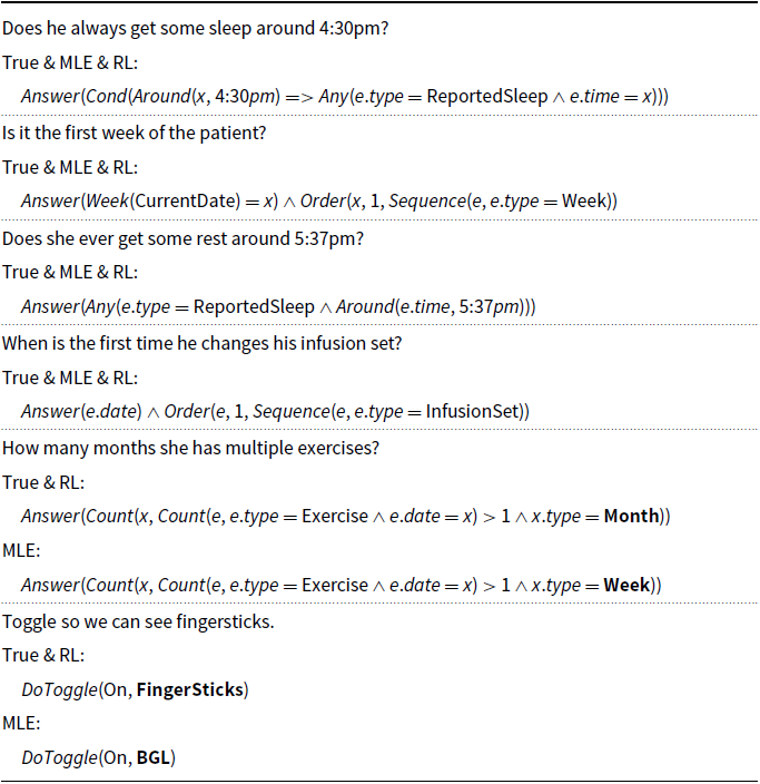
Tables 7 and 8 show examples generated by the SPAAC models on the Frank dataset. Analysis of the generated LFs revealed that one common error made by SPAAC-MLE is the generation of incorrect event types. Some of these errors are fixed by the current RL model. However, there are instances where even the RL-trained model outputs the wrong event type. By comparing the sampled LFs $\hat{Y}^{s}$
and the baseline LFs
$\hat{Y}^{s}$
and the baseline LFs $\hat{Y}^{b}$
, we found that in some cases the tokens for event types in
$\hat{Y}^{b}$
, we found that in some cases the tokens for event types in $\hat{Y}^{s}$
are identical with the wrong event types created in the baseline LFs
$\hat{Y}^{s}$
are identical with the wrong event types created in the baseline LFs $\hat{Y}^{b}$
.
$\hat{Y}^{b}$
.
Table 7. Examples generated by SPAAC-MLE and SPAAC-RL using real interactions. MLE: logical forms by SPAAC-MLE. RL: logical forms by SPAAC-RL. True: manually annotated LFs
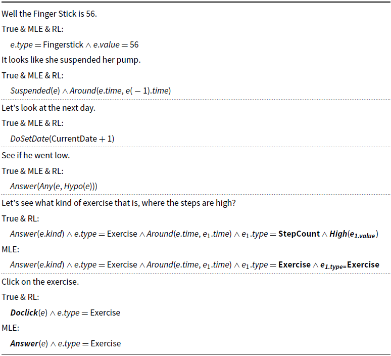
Table 8. Examples generated by SPAAC-MLE and SPAAC-RL using artificial interactions. MLE: logical forms generated by SPAAC-MLE. RL: logical forms generated by SPAAC-RL. True: manually annotated logical forms
4.4.1 Data augmentation
Inspired by the fact that data augmentation improves the performance of speech recognition (Section 3), we applied data augmentation to the semantic parsing system as well. Specifically, we train and test the semantic parsing system, for both models SPAAC-MLE and SPAAC-RL, on the dataset Amber using a 10-fold evaluation scenario similar to the evaluation of the speech recognition system described in Section 3. This system is denoted as SP.Amber (Semantic Parsing of Amber interactions without data augmentation). The dataset Amber is partitioned into 10 equal size folds. For each experiment, nine folds of data are used to train the semantic parsing system and one fold of data is used to evaluate its performance. This process is repeated 10 times, each time using a different fold as test data. The final performance of SP.Amber is computed as the average sequence-level accuracy over the 10 folds. In a second set of experiments, we apply data augmentation to SP.Amber. The system in this evaluation scenario is denoted as SP.Amber + Frank, which means that Amber is the target data and Frank is the external data used for augmentation. In this evaluation scenario, we use the same split in 10 folds as the one used for the SP.Amber experiments. In each experiment, all examples in the Frank dataset are added to the nine folds of data from Amber that are used for training. After training on the nine folds of Amber and the data from Frank, the remaining one fold of data, which comes from the Amber dataset, is used to evaluate the performance of SP.Amber + Frank. The final performance of SP.Amber + Frank is computed as the average sequence-level accuracy over the 10 folds. The results on the Amber data with and without augmentation are shown in the first section of Table 9. To further evaluate the impact of data augmentation, we also run the symmetric evaluation where Frank is the target data and Amber is used as external data. The corresponding results are shown in the second section of Table 9. Finally, we evaluate the semantic parsing system on the union of the two datasets ${Amber \cup Frank}$
, using the same 10-fold evaluation scenario. This system is denoted as SP.All, with its sequence-level accuracy shown in the last section of the table.
${Amber \cup Frank}$
, using the same 10-fold evaluation scenario. This system is denoted as SP.All, with its sequence-level accuracy shown in the last section of the table.
Table 9. Sequence-level accuracy (%) of semantic parsing systems on datasets Amber and Frank. SP.Amber and SP.Frank are the original systems without data augmentation while SP.Amber + Frank and SP.Frank + Amber are the two systems enhanced with data augmentation. SP.All is a system trained and tested on the union of the two datasets
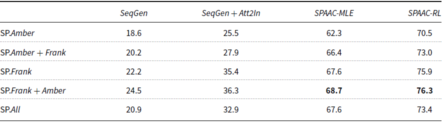
Overall, the results in Table 9 show that data augmentation is beneficial for both models SPAAC-MLE and SPAAC-RL, which continue to do substantially better than the baseline SeqGen. When evaluated on the union of the two datasets, the performance of SP.All is, as expected, between the accuracy obtained by SP.Amber + Frank and SP.Frank + Amber.
Table 10 shows example LFs where data augmentation is able to correct mistakes made by the original SP.Amber and SP.Frank systems.
Table 10. Logical forms generated by SP.Amber + Frank versus SP.Amber, and SP.Frank + Amber versus SP.Frank. True refers to the manually annotated logical forms

Table 11. The performance of the entire semantic parsing pipeline. SP.Amber and SP.Frank are the two systems without data augmentation while SP.Amber + Frank and SP.Frank + Amber are the two systems enhanced with data augmentation. Word error rate (WER) and Sequence-level accuracy (%) are the evaluation metrics

5. Semantic parsing pipeline evaluation
The two main modules of the QA pipeline – speech recognition and semantic parsing – were independently evaluated in Sections 3 and 4, respectively. In this section, we evaluate the performance of the entire semantic parsing pipeline, where the potentially noisy text output by the speech recognizer is used as input for the semantic parsing model. To make results comparable, we used the same 10-fold partition that was used in Sections 3 and 4. The last column in Table 11 shows the sequence-level accuracy of the LFs when running the entire semantic parsing pipeline on the doctors’ speech. Because errors made by the speech recognition system are propagated through the semantic parsing module, the pipeline accuracy is lower than the accuracy of standalone semantic parsing shown in the second column of results. However, inspection of the generated LFs revealed cases where errors introduced by the speech recognition system did not have a negative impact on the final LFs. An example is shown in the first section of Table 12, where the speech recognition system mistakenly transcribes “for” as “a”. However, when run on this slightly erroneous text, the semantic parsing system still generates the correct LF. Another example is shown in the second section, where even though the speech recognition system produces the extra word “again,” the semantic parsing system still outputs the correct LF. The fact that semantic parsing is robust to some speech recognition errors helps explain why SP.Frank is almost as good as SP.Frank + Amber, even though the speech recognizer for SP.Frank makes more errors than the one trained for SP.Frank + Amber. There are, however, cases where the speech recognizer makes multiple errors in the same sentence, as in the example shown in the third section of Table 12, for which the semantic parsing system is unable to recover the correct LF. In this case, instead of returning just one BGL value, corresponding to a particular hyperglycemia event, the system returns all the BGL values recorded that day, which should make it obvious to the user that the system did not understand the question. For this kind of errors, the user has the option to find the correct answer to their query by interacting directly with the GUI using mouse clicks. There are also more subtle errors where the user receives a partially overlapping answer, as shown in the second example from Table 10, where instead of returning all types of discrete events anchored around a certain event, the SP.Amber system returns only Exercise events, at anytime during the day. These types of errors show that, in order to become of practical utility, the system could benefit from features that enabled the user to effortlessly determine whether the query was properly understood. Possible features range from computing and displaying confidence values associated with the outputs, to making the LF computed by the system available to the user, to using explainability methods such as SHAP (Lundberg and Lee Reference Lundberg and Lee2017) that show the inputs that are most responsible for a potentially incorrect LF, thus giving the user the option to reformulate their query or even correct the output in an active learning scenario. While exploring these features is left for future work, we believe that the system described in this paper represents an important first step toward realizing a new QA paradigm in which users express their information needs relative to a GUI using NL queries either exclusively or in combination with direct GUI interactions through mouse clicks.
Table 12. Transcriptions (SR) and logical forms (SP) generated by the pipeline versus corresponding manually annotations (True text and True LF)

6. Related work
Speech Recognition In conventional speech recognition systems, hidden Markov model (HMM)-based approaches and template-based approaches are commonly used (Matarneh et al. Reference Matarneh, Maksymova, Lyashenko and Belova2017). Given a phonetic pronunciation lexicon, the HMM approaches usually operate on the phone level. Handling OOV words is not straightforward and increases the complexity significantly. In recent years, deep learning has been shown to be highly effective in acoustic modeling (Hinton and Salakhutdinov Reference Hinton and Salakhutdinov2006; Bengio Reference Bengio2009; Hinton et al. Reference Hinton, Deng, Yu, Dahl, Mohamed, Jaitly, Senior, Vanhoucke, Nguyen and Kingsbury2012), by employing deep architectures where each layer in the architecture models an increasingly higher-level abstraction of the data. Furthermore, the encoder–decoder framework with neural networks has shown promising results for speech recognition (Chan et al. Reference Chan, Jaitly, Le and Vinyals2016; Doetsch, Zeyer, and Ney Reference Doetsch, Zeyer and Ney2016; Toshniwal et al. Reference Toshniwal, Tang, Lu and Livescu2017; Zeyer et al. Reference Zeyer, Irie, Schlüter and Ney2018; Baskar et al. Reference Baskar, Watanabe, Astudillo, Hori, Burget and Černocký2019; Li et al. Reference Li, Lavrukhin, Ginsburg, Leary, Kuchaiev, Cohen, Nguyen and Gadde2019; Pham et al. Reference Pham, Nguyen, Niehues, Müller and Waibel2019). When trained end-to-end, neural models operate directly on words, subwords, or characters/graphemes, which removes the need for a pronunciation lexicon and explicit phones modeling, highly simplifying decoding, as in Zeyer et al. (Reference Zeyer, Irie, Schlüter and Ney2018). Other models, such as inverted HMMs (Doetsch et al. Reference Doetsch, Hannemann, Schlüter and Ney2017) and the recurrent neural aligner (Sak et al. Reference Sak, Shannon, Rao and Beaufays2017), can be interpreted in the same encoder–decoder framework, but often employ some variant of hard latent monotonic attention instead of soft attention used by Zeyer et al. (Reference Zeyer, Irie, Schlüter and Ney2018).
In our approach, we used fine-tuning to adapt the end-to-end speech recognition of Zeyer et al. (Reference Zeyer, Irie, Schlüter and Ney2018) to the doctors’ speech. This is a straightforward adaptation approach that does not require changing the structure of the adapted module or introducing external modules during inference. Other approaches explore the adaptation of the language model used by the speech recognition system. To accurately estimate the impact of language model adaptation, Mdhaffar et al. (Reference Mdhaffar, Esteve, Hernandez, Laurent, Dufour and Quiniou2019) first perform a qualitative analysis and then conduct experiments on a dataset in French, showing that language model adaptation reduces the WER of speech recognition significantly. Raju et al. (Reference Raju, Filimonov, Tiwari, Lan and Rastrow2019) incorporate a language model into a speech recognition system and train it on heterogenous corpora so that personalized bias is reduced. Corona, Thomason, and Mooney (Reference Corona, Thomason and Mooney2017) incorporate a language model and a semantic parser into a speech recognition system, obtaining a significant improvement over a state-of-the-art baseline in terms of accuracy for both transcription and semantic understanding. Bai et al. (Reference Bai, Yi, Tao, Tian and Wen2019) enhance speech recognition by incorporating a language model via a training approach based on knowledge distillation; the recurrent neural network language model, which is trained on a large corpus, computes a set of soft labels to guide the training of the speech recognition system.
Semantic Parsing, QA, and Context Dependency Semantic parsing, which is mapping text in NL to LFs, has emerged as an important component for building QA systems, as in Liang (Reference Liang2016), Jia and Liang (Reference Jia and Liang2016), Zhong, Xiong, and Socher (Reference Zhong, Xiong and Socher2017). Context-dependent processing has been explored in complex, interactive QA (Harabagiu et al. Reference Harabagiu, Hickl, Lehmann and Moldovan2005; Kelly and Lin Reference Kelly and Lin2007) and semantic parsing (Zettlemoyer and Collins Reference Zettlemoyer and Collins2009; Artzi and Zettlemoyer Reference Artzi and Zettlemoyer2011; Long, Pasupat, and Liang Reference Long, Pasupat and Liang2016; Iyyer, Yih, and Chang Reference Iyyer, Yih and Chang2017). Long et al. (Reference Long, Pasupat and Liang2016) consider the task of learning a context-dependent mapping from NL utterances to denotations in three scenarios: Alchemy, Scene, and Tangrams. Using only denotations at training time, the search space for LFs is much larger than that of the context-dependent utterances. To handle this challenge, the authors perform successive projections of the full model onto simpler models that operate over equivalence classes of LFs. Iyyer et al. (Reference Iyyer, Yih and Chang2017) explore a semantic parsing task for answering sequences of simple but inter-related questions in a conversational QA setting. A dataset of over 6000 question sequences is collected, where each question sequence inquires about semi-structured tables in Wikipedia. To solve this sequential QA task, a novel dynamic neural semantic parsing model is designed, which is trained using a weakly supervised reward guided search. Although these approaches take into account sequential dependencies between questions or sentences, the setting proposed in this paper has a number of significant distinguishing features, such as the importance of time – data are represented naturally as multiple time series of events – and the anchoring on a GUI that enables direct interactions through mouse clicks as well as combinations of factual queries and interface commands.
Dong and Lapata (Reference Dong and Lapata2016) use an attention-enhanced encoder–decoder architecture to learn the LFs from NL without using hand-engineered features. Their proposed Seq2Tree architecture is able to capture the hierarchical structure of LFs. Jia and Liang (Reference Jia and Liang2016) propose a sequence-to-sequence recurrent neural network model where a novel attention-based copying mechanism is used for generating LFs from questions. The copying mechanism has also been investigated by Gulcehre et al. (Reference Gulcehre, Ahn, Nallapati, Zhou and Bengio2016) and Gu et al. (Reference Gu, Lu, Li and Li2016) in the context of a wide range of NLP applications. More recently, Dong and Lapata (Reference Dong and Lapata2018) propose a two-stage semantic parsing architecture, where the first step constructs a rough sketch of the input meaning, which is then completed in the second step by filling in details such as variable names and arguments. One advantage of this approach is that the model can better generalize across examples that have the same sketch, that is, basic meaning. This process could also benefit the models introduced in this paper, where constants such as times and dates would be abstracted out during sketch generation. Another idea that could potentially benefit our context-dependent semantic parsing approach is to rerank an n-best list of predicted LFs based on quality-measuring scores provided by a generative reconstruction model or a discriminative matching model, as was recently proposed by Yin and Neubig (Reference Yin and Neubig2019).
The semantic parsing models above considered sentences in isolation. In contrast, generating correct LFs in our task required modeling sequential dependencies between LFs. In particular, we modeled coreference between events mentioned in different LFs by repurposing the copying mechanism originally used for modeling OOV tokens.
7. Conclusion and future work
We introduced a new QA paradigm in which users can query a system using both NL and direct interactions (mouse clicks) within a GUI. Using medical data acquired from patients with type 1 diabetes as a case study, we proposed a pipeline implementation where a speech recognizer transcribes spoken questions and commands from doctors into a semantically equivalent text that is then semantically parsed into a LF. Once a spoken question has been mapped to its formal representation, its answer can be easily retrieved from the underlying database. The speech recognition module is implemented by adapting a pre-trained LSTM-based architecture to the user’s speech, whereas for the semantic parsing component we introduce an LSTM-based encoder–decoder architecture that models context dependency through copying mechanisms and multiple levels of attention over inputs and previous outputs. Correspondingly, we created a dataset of real interactions and a much larger dataset of artificial interactions. When evaluated separately, with and without data augmentation, both models are shown to substantially outperform several strong baselines. Furthermore, the full pipeline evaluation shows only a limited degradation in semantic parsing accuracy, demonstrating that the semantic parser is robust to mistakes in the speech recognition output. The solution proposed in this paper for the new QA paradigm has the potential for applications in many areas of medicine where large amounts of sensor data and life events are pervasive. The approaches introduced in this paper could also benefit other domains, such as experimental physics, where large amounts of time series data are generated from high-throughput experiments.
Besides the ideas explored in Section 5 for increasing the system’s practical utility, one avenue for future work is to develop an end-to-end neural model which takes the doctor’s spoken questions as input and generates the corresponding LFs directly, instead of producing text as an intermediate representation. Another direction is to jointly train the speech recognition and semantic parsing system, which would enable the speech recognition model to focus on words that are especially important for decoding the correct LF. Finally, expanding the two datasets with more examples of NL interactions is expected to lead to better performance, as well as provide a clearer measure of its performance in a real use scenario.
The two datasets and the implementation of the systems presented in Section 4 are made publicly available at https://github.com/charleschen1015/SemanticParsing. The data visualization GUI is available under the name OhioT1DMViewer at http://smarthealth.cs.ohio.edu/nih.html.
Acknowledgments
This work was partly supported by grant 1R21EB022356 from the National Institutes of Health. We would like to thank Frank Schwartz and Amber Healy for contributing real interactions, Quintin Fettes and Yi Yu for their help with recording and pre-processing the interactions, and Sadegh Mirshekarian for the design of the artificial data generation. We would also like to thank the anonymous reviewers for their constructive comments.
Conflicts of interest
The authors declare none.
A. Artificial Data Generator
An artificial data generator was designed and implemented to simulate doctor–system interactions, with sentence templates defining the skeleton of each entry in order to maintain high-quality sentence structure and grammar. A context free grammar is used to implement a template
Table A1. Examples of generation of artificial samples

language that can specify a virtually unlimited number of templates and generate as many examples as desired. Below we show a simplification of three sample rules from the grammar:
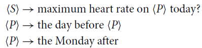 \begin{align}\langle S \rangle &\rightarrow \mbox{maximum heart rate on } \langle P \rangle \mbox{ today}? \nonumber\\\langle P \rangle &\rightarrow \mbox{the day before } \langle P \rangle \nonumber\\\langle P \rangle &\rightarrow \mbox{the Monday after} \nonumber\end{align}
A sample derivation using these rules is “maximum heart rate on the Monday after today?”.
The implementation allows for the definition of any number of non-terminals, which are called types, and any number of templates, which are the possible right-hand sides of the starting symbol S. The doctor–system interactions can be categorized into three types: questions, statements, and clicks, where templates can be defined for each type, as shown in Table A1. Given the set of types and templates, a virtually unlimited number of sentences can be derived to form the artificial dataset. Since the sentence generator chooses each template randomly, the order of sentences in the output dataset will be random. However, two important aspects of the real interactions are context dependency and coreference. To achieve context dependency, the implementation allows for more complex combo templates where multiple templates are forced to come in a predefined order. It is also possible to specify groups of templates, via tagging, and combine groups rather than individual templates. Furthermore, each NL sentence template is paired with a LF template, and the two templates are instantiated jointly, using a reference mechanism to condition the logical form generation on decisions made while deriving the sentence.
Table A1 shows examples of how artificial sentences and their logical forms are generated given templates and types. Most types are defined using context free rules. There are, however, special types, such as [clocktime] and [range()], which are dynamically rewritten as a random time and a random integer from a given range, as shown in Examples 3 and 4, respectively. Note that most examples use referencing, which is a mechanism to allow for dynamic matching of terminals between the NL and LF derivations. In Example 1, $\$1$
in the logical form template refers to the first type in the main sentence, which is [week_days]. This means that whatever value is substituted for [week_days] should appear verbatim in place of
$\$1$
in the logical form template refers to the first type in the main sentence, which is [week_days]. This means that whatever value is substituted for [week_days] should appear verbatim in place of $\$1$
. In case a coordinated matching from a separate list of possible options is required, such as in Example 2, another type can be selected. In Example 2, [
$\$1$
. In case a coordinated matching from a separate list of possible options is required, such as in Example 2, another type can be selected. In Example 2, [ ${\$}$
2:any_event_logic] will be option i from the type [any_event_logic] when option i is chosen in the main sentence for the second template, which is [any_event].
${\$}$
2:any_event_logic] will be option i from the type [any_event_logic] when option i is chosen in the main sentence for the second template, which is [any_event].


 Open access