


 defined by homogeneous forms


1 Introduction
Let
 $k$
be a field. We investigate rational maps
$k$
be a field. We investigate rational maps  Such a map
 $\unicode[STIX]{x1D6F9}$
is defined by homogeneous forms
$\unicode[STIX]{x1D6F9}$
is defined by homogeneous forms
 $g_{1},\ldots ,g_{n}$
, of the same degree
$g_{1},\ldots ,g_{n}$
, of the same degree
 $d$
, in the homogeneous coordinate ring
$d$
, in the homogeneous coordinate ring
 $R=k[x_{1},\ldots ,x_{s}]$
of
$R=k[x_{1},\ldots ,x_{s}]$
of
 $\mathbb{P}_{k}^{s-1}$
. One of our main goals is to determine necessary and sufficient conditions for
$\mathbb{P}_{k}^{s-1}$
. One of our main goals is to determine necessary and sufficient conditions for
 $\unicode[STIX]{x1D6F9}$
to be birational onto its image. This problem has been studied extensively; see, for example, Hacon [Reference Hacon22] for a technique that uses the nonvanishing theorem of Kollár [Reference Kollár35]. The advantage of having convenient criteria for determining if a given parameterization is birational onto its image is quite obvious. Papers about parameterization of curves and surfaces are now ubiquitous (see, for example [Reference Cortadellas Benitez and D’Andrea2–Reference Botbol, Busé and Chardin4, Reference Busé7–Reference Chen, Wang and Liu11, Reference Cox, Hoffman and Wang15, Reference Cox, Kustin, Polini and Ulrich16, Reference Hong, Simis and Vasconcelos24, Reference Hong, Simis and Vasconcelos25, Reference Kustin, Polini and Ulrich37, Reference Song, Chen and Goldman50]). It is much better to have “the parameterization is birational” as a conclusion, rather than as a hypothesis.
$\unicode[STIX]{x1D6F9}$
to be birational onto its image. This problem has been studied extensively; see, for example, Hacon [Reference Hacon22] for a technique that uses the nonvanishing theorem of Kollár [Reference Kollár35]. The advantage of having convenient criteria for determining if a given parameterization is birational onto its image is quite obvious. Papers about parameterization of curves and surfaces are now ubiquitous (see, for example [Reference Cortadellas Benitez and D’Andrea2–Reference Botbol, Busé and Chardin4, Reference Busé7–Reference Chen, Wang and Liu11, Reference Cox, Hoffman and Wang15, Reference Cox, Kustin, Polini and Ulrich16, Reference Hong, Simis and Vasconcelos24, Reference Hong, Simis and Vasconcelos25, Reference Kustin, Polini and Ulrich37, Reference Song, Chen and Goldman50]). It is much better to have “the parameterization is birational” as a conclusion, rather than as a hypothesis.
In this paper we employ the syzygies of the forms
 $[g_{1},\ldots ,g_{n}]$
to determine if the rational map
$[g_{1},\ldots ,g_{n}]$
to determine if the rational map  is birational. For
 $s=n$
this approach appears already in the work of Hulek et al. [Reference Hulek, Katz and Schreyer26], and for
$s=n$
this approach appears already in the work of Hulek et al. [Reference Hulek, Katz and Schreyer26], and for
 $n\geqslant s$
it has been further developed in [Reference Russo and Simis47]. In [Reference Doria, Hassanzadeh and Simis17, Reference Simis48] the method has been advanced by emphasizing the role of the Rees algebra associated to the ideal
$n\geqslant s$
it has been further developed in [Reference Russo and Simis47]. In [Reference Doria, Hassanzadeh and Simis17, Reference Simis48] the method has been advanced by emphasizing the role of the Rees algebra associated to the ideal
 $I=(g_{1},\ldots ,g_{n})$
of
$I=(g_{1},\ldots ,g_{n})$
of
 $R$
. The Rees algebra
$R$
. The Rees algebra
 ${\mathcal{R}}(I)$
gives the bihomogeneous coordinate ring of the graph of
${\mathcal{R}}(I)$
gives the bihomogeneous coordinate ring of the graph of
 $\unicode[STIX]{x1D6F9}$
, whereas, the subalgebra
$\unicode[STIX]{x1D6F9}$
, whereas, the subalgebra
 $A=k[g_{1},\ldots ,g_{n}]$
of
$A=k[g_{1},\ldots ,g_{n}]$
of
 $R$
is the homogeneous coordinate ring of the image of
$R$
is the homogeneous coordinate ring of the image of
 $\unicode[STIX]{x1D6F9}$
. In fact,
$\unicode[STIX]{x1D6F9}$
. In fact,
 $A$
is isomorphic to the special fiber ring
$A$
is isomorphic to the special fiber ring
 ${\mathcal{F}}(I)={\mathcal{R}}(I)/\mathfrak{m}{\mathcal{R}}(I)$
for
${\mathcal{F}}(I)={\mathcal{R}}(I)/\mathfrak{m}{\mathcal{R}}(I)$
for
 $\mathfrak{m}$
equal to the maximal homogeneous ideal
$\mathfrak{m}$
equal to the maximal homogeneous ideal
 $\mathfrak{m}=(x_{1},\ldots ,x_{s})$
of
$\mathfrak{m}=(x_{1},\ldots ,x_{s})$
of
 $R$
. The rings
$R$
. The rings
 ${\mathcal{R}}(I)$
and
${\mathcal{R}}(I)$
and
 ${\mathcal{F}}(I)$
are known as blowup rings associated to
${\mathcal{F}}(I)$
are known as blowup rings associated to
 $I$
. In this paper we relate geometric properties of
$I$
. In this paper we relate geometric properties of
 $\unicode[STIX]{x1D6F9}$
, algebraic information about the homogeneous coordinate ring
$\unicode[STIX]{x1D6F9}$
, algebraic information about the homogeneous coordinate ring
 $A$
of the image, and the bihomogeneous coordinate ring
$A$
of the image, and the bihomogeneous coordinate ring
 ${\mathcal{R}}(I)$
of the graph.
${\mathcal{R}}(I)$
of the graph.
If
 $\unicode[STIX]{x1D6F9}$
is a morphism (that is, if
$\unicode[STIX]{x1D6F9}$
is a morphism (that is, if
 $I$
is primary to the maximal homogeneous ideal
$I$
is primary to the maximal homogeneous ideal
 $\mathfrak{m}$
of
$\mathfrak{m}$
of
 $R$
), then the degree of
$R$
), then the degree of
 $\unicode[STIX]{x1D6F9}:\mathbb{P}_{k}^{s-1}\rightarrow \operatorname{Im}\unicode[STIX]{x1D6F9}$
is equal to
$\unicode[STIX]{x1D6F9}:\mathbb{P}_{k}^{s-1}\rightarrow \operatorname{Im}\unicode[STIX]{x1D6F9}$
is equal to
 $d^{s-1}/e(A)$
, where
$d^{s-1}/e(A)$
, where
 $e(A)$
is the multiplicity of the standard-graded
$e(A)$
is the multiplicity of the standard-graded
 $k$
-algebra
$k$
-algebra
 $A$
. We prove, for instance, that
$A$
. We prove, for instance, that
 ${\mathcal{R}}(I)$
satisfies Serre’s condition
${\mathcal{R}}(I)$
satisfies Serre’s condition
 $R_{i}$
, for some
$R_{i}$
, for some
 $i>0$
, if and only if
$i>0$
, if and only if
 $A$
satisfies
$A$
satisfies
 $R_{i-1}$
and
$R_{i-1}$
and
 $\unicode[STIX]{x1D6F9}$
is birational onto its image (that is,
$\unicode[STIX]{x1D6F9}$
is birational onto its image (that is,
 $\unicode[STIX]{x1D6F9}:\mathbb{P}_{k}^{s-1}\rightarrow \operatorname{Im}\unicode[STIX]{x1D6F9}$
has degree
$\unicode[STIX]{x1D6F9}:\mathbb{P}_{k}^{s-1}\rightarrow \operatorname{Im}\unicode[STIX]{x1D6F9}$
has degree
 $1$
). Thus, in particular,
$1$
). Thus, in particular,
 $\unicode[STIX]{x1D6F9}$
is birational onto its image if and only if
$\unicode[STIX]{x1D6F9}$
is birational onto its image if and only if
 ${\mathcal{R}}(I)$
satisfies
${\mathcal{R}}(I)$
satisfies
 $R_{1}$
. Furthermore,
$R_{1}$
. Furthermore,
 $\unicode[STIX]{x1D6F9}:\mathbb{P}_{k}^{s-1}\rightarrow \operatorname{Im}\unicode[STIX]{x1D6F9}$
is a birational morphism with a smooth image if and only if the Rees ring
$\unicode[STIX]{x1D6F9}:\mathbb{P}_{k}^{s-1}\rightarrow \operatorname{Im}\unicode[STIX]{x1D6F9}$
is a birational morphism with a smooth image if and only if the Rees ring
 ${\mathcal{R}}(I)$
has an isolated singularity. Even if the rational map
${\mathcal{R}}(I)$
has an isolated singularity. Even if the rational map
 $\unicode[STIX]{x1D6F9}$
is not a morphism, if the dimension of
$\unicode[STIX]{x1D6F9}$
is not a morphism, if the dimension of
 $\operatorname{Im}\unicode[STIX]{x1D6F9}$
is
$\operatorname{Im}\unicode[STIX]{x1D6F9}$
is
 $s-1$
(that is, if the Krull dimension of
$s-1$
(that is, if the Krull dimension of
 $A$
is
$A$
is
 $s$
), then the degree of
$s$
), then the degree of
 $\unicode[STIX]{x1D6F9}:\mathbb{P}_{k}^{s-1}\rightarrow \operatorname{Im}\unicode[STIX]{x1D6F9}$
is equal to the multiplicity of the local ring
$\unicode[STIX]{x1D6F9}:\mathbb{P}_{k}^{s-1}\rightarrow \operatorname{Im}\unicode[STIX]{x1D6F9}$
is equal to the multiplicity of the local ring
 ${\mathcal{R}}(I)_{\mathfrak{m}{\mathcal{R}}(I)}$
. Moreover, we are able to relate the degree of the map
${\mathcal{R}}(I)_{\mathfrak{m}{\mathcal{R}}(I)}$
. Moreover, we are able to relate the degree of the map
 $\unicode[STIX]{x1D6F9}$
, the degree of the image, and the
$\unicode[STIX]{x1D6F9}$
, the degree of the image, and the
 $j$
-multiplicity of the ideal
$j$
-multiplicity of the ideal
 $I$
. Results of this type were obtained before by Simis et al. [Reference Simis, Ulrich and Vasconcelos49], Validashti [Reference Validashti52], Xie [Reference Xie53] and by Jeffries et al. [Reference Jeffries, Montaño and Varbaro32].
$I$
. Results of this type were obtained before by Simis et al. [Reference Simis, Ulrich and Vasconcelos49], Validashti [Reference Validashti52], Xie [Reference Xie53] and by Jeffries et al. [Reference Jeffries, Montaño and Varbaro32].
The
 $j$
-multiplicity is a generalization of the classical Hilbert–Samuel multiplicity that applies to ideals that are not necessarily zero-dimensional. The notion was introduced by Achilles and Manaresi [Reference Achilles and Manaresi1] and has found applications in intersection theory and equisingularity theory. It is interesting to find formulas for the
$j$
-multiplicity is a generalization of the classical Hilbert–Samuel multiplicity that applies to ideals that are not necessarily zero-dimensional. The notion was introduced by Achilles and Manaresi [Reference Achilles and Manaresi1] and has found applications in intersection theory and equisingularity theory. It is interesting to find formulas for the
 $j$
-multiplicity of classes of ideals [Reference Jeffries and Montaño31, Reference Jeffries, Montaño and Varbaro32, Reference Nishida and Ulrich42]. Our formula serves this purpose if the degree of the map and of its image are known. Conversely, we obtain the degree of the image of a rational map if the
$j$
-multiplicity of classes of ideals [Reference Jeffries and Montaño31, Reference Jeffries, Montaño and Varbaro32, Reference Nishida and Ulrich42]. Our formula serves this purpose if the degree of the map and of its image are known. Conversely, we obtain the degree of the image of a rational map if the
 $j$
-multiplicity can be computed, for instance by using residual intersection techniques (see, e.g. [Reference Kustin, Polini and Ulrich38]). We also express the degree of certain dual varieties in terms of the
$j$
-multiplicity can be computed, for instance by using residual intersection techniques (see, e.g. [Reference Kustin, Polini and Ulrich38]). We also express the degree of certain dual varieties in terms of the
 $j$
-multiplicity of Jacobian ideals.
$j$
-multiplicity of Jacobian ideals.
The starting point for our investigation is the Eisenbud–Ulrich interpretation [Reference Eisenbud and Ulrich19] of the fibers of the morphism
 $\unicode[STIX]{x1D6F9}$
over the point
$\unicode[STIX]{x1D6F9}$
over the point
 $p$
in
$p$
in
 $\mathbb{P}^{n-1}$
in terms of the corresponding generalized row of the homogeneous syzygy matrix for
$\mathbb{P}^{n-1}$
in terms of the corresponding generalized row of the homogeneous syzygy matrix for
 $[g_{1},\ldots ,g_{n}]$
. This technique is explained and extended in Section 3; it also plays a significant role in [Reference Cox, Kustin, Polini and Ulrich16].
$[g_{1},\ldots ,g_{n}]$
. This technique is explained and extended in Section 3; it also plays a significant role in [Reference Cox, Kustin, Polini and Ulrich16].
In Section 4, we prove an algebraic analogue of a consequence of Hurwitz’ theorem. Let
 $r$
be the degree of the morphism
$r$
be the degree of the morphism  which at the level of coordinate rings corresponds to the embedding
 $A{\hookrightarrow}k[R_{d}]$
. Thus
$A{\hookrightarrow}k[R_{d}]$
. Thus
 $r$
is the degree of the field extension
$r$
is the degree of the field extension
 $\text{Quot}(A)\subset \text{Quot}(k[R_{d}])$
. We show that there exist homogeneous forms
$\text{Quot}(A)\subset \text{Quot}(k[R_{d}])$
. We show that there exist homogeneous forms
 $f_{1},f_{2}$
of degree
$f_{1},f_{2}$
of degree
 $r$
in
$r$
in
 $R$
such that the entries of the matrix
$R$
such that the entries of the matrix
 $\unicode[STIX]{x1D711}$
are homogeneous polynomials in the variables
$\unicode[STIX]{x1D711}$
are homogeneous polynomials in the variables
 $f_{1}$
and
$f_{1}$
and
 $f_{2}$
. In particular, the ideal
$f_{2}$
. In particular, the ideal
 $I$
is extended from an ideal in
$I$
is extended from an ideal in
 $k[f_{1},f_{2}]$
. Thus, replacing
$k[f_{1},f_{2}]$
. Thus, replacing
 $k[x_{1},x_{2}]$
by
$k[x_{1},x_{2}]$
by
 $k[f_{1},f_{2}]$
we can reduce the nonbirational case to the birational one. Furthermore, we provide an explicit description of
$k[f_{1},f_{2}]$
we can reduce the nonbirational case to the birational one. Furthermore, we provide an explicit description of
 $f_{1}$
and
$f_{1}$
and
 $f_{2}$
in terms of
$f_{2}$
in terms of
 $\unicode[STIX]{x1D711}$
. If
$\unicode[STIX]{x1D711}$
. If
 $q_{1}$
and
$q_{1}$
and
 $q_{2}$
are general points in
$q_{2}$
are general points in
 $\mathbb{P}_{k}^{1}$
, then
$\mathbb{P}_{k}^{1}$
, then
 $f_{i}=\text{gcd}(I_{1}(p_{i}\unicode[STIX]{x1D711}))$
with
$f_{i}=\text{gcd}(I_{1}(p_{i}\unicode[STIX]{x1D711}))$
with
 $p_{i}=\unicode[STIX]{x1D6F9}(q_{i})$
. This method gives an efficient algorithm for reparameterizing the rational map
$p_{i}=\unicode[STIX]{x1D6F9}(q_{i})$
. This method gives an efficient algorithm for reparameterizing the rational map
 $\unicode[STIX]{x1D6F9}$
.
$\unicode[STIX]{x1D6F9}$
.
In Section 5, we relate the birationality of
 $\unicode[STIX]{x1D6F9}$
to the shape of
$\unicode[STIX]{x1D6F9}$
to the shape of
 $\operatorname{core}(I)$
, the core of
$\operatorname{core}(I)$
, the core of
 $I$
, the intersection of all reductions of
$I$
, the intersection of all reductions of
 $I$
. Since reductions, even minimal ones, are highly nonunique, one uses the core to encode information about all of them. The concept was introduced by Rees and Sally [Reference Rees and Sally46], and has been studied further by Huneke and Swanson, by Corso, Polini, and Ulrich, by Polini and Ulrich, and by Huneke and Trung [Reference Corso, Polini and Ulrich12–Reference Corso, Polini and Ulrich14, Reference Huneke and Swanson27, Reference Huneke and Trung28, Reference Polini and Ulrich44]. The core appears naturally in the contexts of Briançon–Skoda theorems that compare the integral closure filtration with the adic filtration of an ideal [Reference Briançon and Skoda6, Reference Lipman40]. Another aspect that makes the core very appealing is its connection to adjoints and multiplier ideals, and, as discovered by Hyry and Smith, to Kawamata’s conjecture on the nonvanishing of sections of certain line bundles [Reference Hyry and Smith29, Reference Hyry and Smith30]. We prove that if
$I$
. Since reductions, even minimal ones, are highly nonunique, one uses the core to encode information about all of them. The concept was introduced by Rees and Sally [Reference Rees and Sally46], and has been studied further by Huneke and Swanson, by Corso, Polini, and Ulrich, by Polini and Ulrich, and by Huneke and Trung [Reference Corso, Polini and Ulrich12–Reference Corso, Polini and Ulrich14, Reference Huneke and Swanson27, Reference Huneke and Trung28, Reference Polini and Ulrich44]. The core appears naturally in the contexts of Briançon–Skoda theorems that compare the integral closure filtration with the adic filtration of an ideal [Reference Briançon and Skoda6, Reference Lipman40]. Another aspect that makes the core very appealing is its connection to adjoints and multiplier ideals, and, as discovered by Hyry and Smith, to Kawamata’s conjecture on the nonvanishing of sections of certain line bundles [Reference Hyry and Smith29, Reference Hyry and Smith30]. We prove that if
 $\unicode[STIX]{x1D6F9}$
is birational onto its image then
$\unicode[STIX]{x1D6F9}$
is birational onto its image then
 $\text{core}(I)$
is the adjoint ideal of
$\text{core}(I)$
is the adjoint ideal of
 $I^{s}$
and
$I^{s}$
and
 $\text{core}(I)=(x_{1},\ldots ,x_{s})^{sd-s+1}$
. The converse of this statement holds for
$\text{core}(I)=(x_{1},\ldots ,x_{s})^{sd-s+1}$
. The converse of this statement holds for
 $s=2$
. Indeed, if
$s=2$
. Indeed, if
 $\operatorname{Im}\unicode[STIX]{x1D6F9}$
is a curve,
$\operatorname{Im}\unicode[STIX]{x1D6F9}$
is a curve,
 $\unicode[STIX]{x1D6F9}$
is a morphism, and
$\unicode[STIX]{x1D6F9}$
is a morphism, and
 $\unicode[STIX]{x1D711}$
is a homogeneous Hilbert–Burch matrix for the row vector
$\unicode[STIX]{x1D711}$
is a homogeneous Hilbert–Burch matrix for the row vector
 $[g_{1},\ldots ,g_{n}]$
, then in 5.14 we prove the following result.
$[g_{1},\ldots ,g_{n}]$
, then in 5.14 we prove the following result.
Theorem.
Statements (1)–(8) are equivalent.
-
(1) The morphism
 $\,\unicode[STIX]{x1D6F9}$
is birational onto its image.
$\,\unicode[STIX]{x1D6F9}$
is birational onto its image. -
(2) The Rees ring
${\mathcal{R}}(I)$
satisfies Serre’s condition
$(R_{1})$
. -
(3) One has the equality of canonical modules
$\unicode[STIX]{x1D714}_{{\mathcal{R}}(I)}=\unicode[STIX]{x1D714}_{{\mathcal{R}}(\mathfrak{m}^{d})}$
. -
(4) One has the equality of endomorphism rings
$$\begin{eqnarray}\operatorname{End}_{{\mathcal{R}}(I)}(\unicode[STIX]{x1D714}_{{\mathcal{R}}(I)})=\operatorname{End}_{{\mathcal{R}}(\mathfrak{m}^{d})}(\unicode[STIX]{x1D714}_{{\mathcal{R}}(\mathfrak{m}^{d})}).\end{eqnarray}$$
-
(5)
$e(A)=d$
. -
(6)
$\text{core}(I)=\mathfrak{m}^{2d-1}$
. -
(7) One has the equality of the core and an adjoint
$\text{core}(I)=\text{adj}(I^{2})$
. -
(8) The ideal
$\text{core}(I)$
is integrally closed.Furthermore, statements (1)–(8) are all implied by
-
(9)
$\gcd (\text{column degrees of }\unicode[STIX]{x1D711})=1$
.


We highlight the fact that the integral closedness of the core of
 $I$
, which is a single graded component of the canonical module
$I$
, which is a single graded component of the canonical module
 $\unicode[STIX]{x1D714}_{{\mathcal{R}}(I)}$
, forces the shape of the entire canonical module. Also, we emphasize that these equivalent conditions may sometimes be read from numerical information about a homogeneous presentation matrix
$\unicode[STIX]{x1D714}_{{\mathcal{R}}(I)}$
, forces the shape of the entire canonical module. Also, we emphasize that these equivalent conditions may sometimes be read from numerical information about a homogeneous presentation matrix
 $\unicode[STIX]{x1D711}$
for
$\unicode[STIX]{x1D711}$
for
 $I$
(that is, from information about the graded Betti numbers of the homogeneous ideal
$I$
(that is, from information about the graded Betti numbers of the homogeneous ideal
 $I$
in the ring
$I$
in the ring
 $R=k[x_{1},x_{2}]$
). In general, the sufficient condition (9) is far from necessary; however, if
$R=k[x_{1},x_{2}]$
). In general, the sufficient condition (9) is far from necessary; however, if
 $I$
is generated by monomials, then condition (9) is equivalent to conditions (1)–(8).
$I$
is generated by monomials, then condition (9) is equivalent to conditions (1)–(8).
The fact that the core can detect geometric properties was already apparent in the work of Hyry and Smith [Reference Hyry and Smith29, Reference Hyry and Smith30] and in [Reference Fouli, Polini and Ulrich20], where the Cayley–Bacharach property of zero-dimensional schemes is characterized in terms of the structure of the core of the maximal ideal of their homogeneous coordinate ring. The equality
 $\text{core}(I)=\text{adj}(I^{g})$
(where
$\text{core}(I)=\text{adj}(I^{g})$
(where
 $g$
is the height of the ideal
$g$
is the height of the ideal
 $I$
) has also been investigated by Hyry and Smith [Reference Hyry and Smith29, Reference Hyry and Smith30] in their work on the conjecture of Kawamata. Adjoints of ideals in regular domains were introduced by Lipman [Reference Lipman40], and in rings essentially of finite type over a field of characteristic zero they coincide with multiplier ideals, which play an important role in algebraic geometry due to their connection with vanishing theorems [Reference Lazarsfeld39]. For the core to be the adjoint of an ideal, it needs to be integrally closed, which is always the case if
$I$
) has also been investigated by Hyry and Smith [Reference Hyry and Smith29, Reference Hyry and Smith30] in their work on the conjecture of Kawamata. Adjoints of ideals in regular domains were introduced by Lipman [Reference Lipman40], and in rings essentially of finite type over a field of characteristic zero they coincide with multiplier ideals, which play an important role in algebraic geometry due to their connection with vanishing theorems [Reference Lazarsfeld39]. For the core to be the adjoint of an ideal, it needs to be integrally closed, which is always the case if
 ${\mathcal{R}}(I)$
satisfies Serre’s condition
${\mathcal{R}}(I)$
satisfies Serre’s condition
 $R_{1}$
(see [Reference Polini and Ulrich44]). Surprisingly, however, in 5.14 the integral closeness of the core is sufficient to guarantee the equality between the core and the multiplier ideal.
$R_{1}$
(see [Reference Polini and Ulrich44]). Surprisingly, however, in 5.14 the integral closeness of the core is sufficient to guarantee the equality between the core and the multiplier ideal.
2 Notation, conventions, and preliminary results
2.1. If
 $I$
and
$I$
and
 $J$
are ideals of a ring
$J$
are ideals of a ring
 $R$
, then the saturation of
$R$
, then the saturation of
 $I$
with respect to
$I$
with respect to
 $J$
is
$J$
is
 $I:J^{\infty }=\bigcup _{i=1}^{\infty }(I:J^{i})$
. Recall that
$I:J^{\infty }=\bigcup _{i=1}^{\infty }(I:J^{i})$
. Recall that
 $I:J^{\infty }$
is obtained from
$I:J^{\infty }$
is obtained from
 $I$
by removing all primary components whose radical contain
$I$
by removing all primary components whose radical contain
 $J$
. We write
$J$
. We write
 $\text{gcd}$
to mean greatest common divisor. If
$\text{gcd}$
to mean greatest common divisor. If
 $I$
is a homogeneous ideal in
$I$
is a homogeneous ideal in
 $k[x,y]$
, then we denote the
$k[x,y]$
, then we denote the
 $\text{gcd}$
of a generating set of
$\text{gcd}$
of a generating set of
 $I$
by
$I$
by
 $\text{gcd}(I)$
; notice that this polynomial generates the saturation
$\text{gcd}(I)$
; notice that this polynomial generates the saturation
 $I:(x,y)^{\infty }$
.
$I:(x,y)^{\infty }$
.
2.2. If
 $R$
is a ring, then we write
$R$
is a ring, then we write
 $\operatorname{Quot}(R)$
for the total ring of quotients of
$\operatorname{Quot}(R)$
for the total ring of quotients of
 $R$
; that is,
$R$
; that is,
 $$\begin{eqnarray}\operatorname{Quot}(R)=U^{-1}R,\end{eqnarray}$$
where
 $U$
is the set of nonzerodivisors on
$U$
is the set of nonzerodivisors on
 $R$
. If
$R$
. If
 $R$
is a domain, then the total ring of quotients of
$R$
is a domain, then the total ring of quotients of
 $R$
is usually called the quotient field of
$R$
is usually called the quotient field of
 $R$
. An extension of domains
$R$
. An extension of domains
 $A\subset B$
is called birational if
$A\subset B$
is called birational if
 $A$
and
$A$
and
 $B$
have the same quotient field.
$B$
have the same quotient field.
If
 $A\subset B$
is an extension of domains so that
$A\subset B$
is an extension of domains so that
 $\operatorname{Quot}(B)$
is algebraic over
$\operatorname{Quot}(B)$
is algebraic over
 $\operatorname{Quot}(A)$
, then we use the three notations
$\operatorname{Quot}(A)$
, then we use the three notations
 $$\begin{eqnarray}[B:A],\quad \operatorname{rank}_{A}B,\quad \text{and}\quad [\operatorname{Quot}(B):\operatorname{Quot}(A)]\end{eqnarray}$$
interchangeably. Indeed, in this situation,
 $$\begin{eqnarray}\operatorname{Quot}(A)\otimes _{A}B=\operatorname{Quot}(B).\end{eqnarray}$$
The rank of
 $B$
as an
$B$
as an
 $A$
-module, denoted
$A$
-module, denoted
 $\operatorname{rank}_{A}B$
, is defined to be the dimension of the left hand side of (2.2.1) as a vector space over
$\operatorname{rank}_{A}B$
, is defined to be the dimension of the left hand side of (2.2.1) as a vector space over
 $\operatorname{Quot}(A)$
. The dimension of the right side of (2.2.1), as a vector space over
$\operatorname{Quot}(A)$
. The dimension of the right side of (2.2.1), as a vector space over
 $\operatorname{Quot}(A)$
, is denoted
$\operatorname{Quot}(A)$
, is denoted
 $[\operatorname{Quot}(B):\operatorname{Quot}(A)]$
.
$[\operatorname{Quot}(B):\operatorname{Quot}(A)]$
.
2.3. If
 $R$
is a Noetherian ring,
$R$
is a Noetherian ring,
 $M$
is a finitely generated
$M$
is a finitely generated
 $R$
-module of Krull dimension
$R$
-module of Krull dimension
 $s$
, and
$s$
, and
 $\mathfrak{a}$
is an ideal of
$\mathfrak{a}$
is an ideal of
 $R$
with the Krull dimension of
$R$
with the Krull dimension of
 $R/\mathfrak{a}$
equal to zero, then the multiplicity of the
$R/\mathfrak{a}$
equal to zero, then the multiplicity of the
 $R$
-module
$R$
-module
 $M$
with respect to the ideal
$M$
with respect to the ideal
 $\mathfrak{a}$
is
$\mathfrak{a}$
is
 $$\begin{eqnarray}e_{\mathfrak{a}}(M)=s!\lim _{n\rightarrow \infty }\frac{\unicode[STIX]{x1D706}_{R}(M/\mathfrak{a}^{n}M)}{n^{s}},\end{eqnarray}$$
where
 $\unicode[STIX]{x1D706}_{R}(\underline{\phantom{x}})$
represents the length of an
$\unicode[STIX]{x1D706}_{R}(\underline{\phantom{x}})$
represents the length of an
 $R$
-module. If
$R$
-module. If
 $R$
is local with maximal ideal
$R$
is local with maximal ideal
 $\mathfrak{m}$
, then we often write
$\mathfrak{m}$
, then we often write
 $e(M)$
or
$e(M)$
or
 $e_{R}(M)$
in place of
$e_{R}(M)$
in place of
 $e_{\mathfrak{m}}(M)$
. Similarly, if
$e_{\mathfrak{m}}(M)$
. Similarly, if
 $R$
is a standard-graded algebra over a field (see 2.4) with maximal homogeneous ideal
$R$
is a standard-graded algebra over a field (see 2.4) with maximal homogeneous ideal
 $\mathfrak{m}$
, and
$\mathfrak{m}$
, and
 $M$
is a graded
$M$
is a graded
 $R$
-module, then we often write
$R$
-module, then we often write
 $e(M)$
or
$e(M)$
or
 $e_{R}(M)$
in place of
$e_{R}(M)$
in place of
 $e_{\mathfrak{m}}(M)$
. In either case, we call the common value
$e_{\mathfrak{m}}(M)$
. In either case, we call the common value
 $e(M)=e_{R}(M)=e_{\mathfrak{m}}(M)$
the multiplicity of the
$e(M)=e_{R}(M)=e_{\mathfrak{m}}(M)$
the multiplicity of the
 $R$
-module
$R$
-module
 $M$
; in particular,
$M$
; in particular,
 $e(R)$
means
$e(R)$
means
 $e_{R}(R)$
.
$e_{R}(R)$
.
2.4. Let
 $R=\bigoplus _{0\leqslant i}R_{i}$
be a Noetherian graded algebra and
$R=\bigoplus _{0\leqslant i}R_{i}$
be a Noetherian graded algebra and
 $M$
be a finitely generated graded
$M$
be a finitely generated graded
 $R$
-module. It follows that
$R$
-module. It follows that
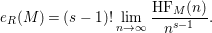
 $$\begin{eqnarray}\unicode[STIX]{x1D706}_{R_{0}}(M_{n})=\unicode[STIX]{x1D706}_{R}\left(\frac{\underset{n\leqslant i}{\bigoplus }M_{i}}{\underset{n<i}{\bigoplus }M_{i}}\right).\end{eqnarray}$$
This nonnegative integer is the value of the Hilbert function of the
 $R$
-module
$R$
-module
 $M$
at
$M$
at
 $n$
, denoted
$n$
, denoted
 $\operatorname{HF}_{M}(n)$
.
$\operatorname{HF}_{M}(n)$
.
Let
 $k$
be a field. The graded algebra
$k$
be a field. The graded algebra
 $R=\bigoplus _{0\leqslant i}R_{i}$
is a standard-graded
$R=\bigoplus _{0\leqslant i}R_{i}$
is a standard-graded
 $k$
-algebra if
$k$
-algebra if
 $R_{0}$
is equal to
$R_{0}$
is equal to
 $k$
,
$k$
,
 $R_{1}$
is a finitely generated
$R_{1}$
is a finitely generated
 $R_{0}$
-module, and
$R_{0}$
-module, and
 $R$
is generated by
$R$
is generated by
 $R_{1}$
as an algebra over
$R_{1}$
as an algebra over
 $R_{0}$
. If
$R_{0}$
. If
 $R$
is a standard-graded
$R$
is a standard-graded
 $k$
-algebra and
$k$
-algebra and
 $M$
is a finitely generated, graded
$M$
is a finitely generated, graded
 $R$
-module with positive Krull dimension
$R$
-module with positive Krull dimension
 $s$
, then the multiplicity of
$s$
, then the multiplicity of
 $M$
may be expressed in terms of Hilbert functions:
$M$
may be expressed in terms of Hilbert functions:
 $$\begin{eqnarray}e_{R}(M)=(s-1)!\lim _{n\rightarrow \infty }\frac{\operatorname{HF}_{M}(n)}{n^{s-1}}.\end{eqnarray}$$
2.5. If
 $R$
is a standard-graded
$R$
is a standard-graded
 $k$
-algebra with maximal homogeneous ideal
$k$
-algebra with maximal homogeneous ideal
 $\mathfrak{m}$
, then the multiplicity
$\mathfrak{m}$
, then the multiplicity
 $e(R)$
of the standard-graded
$e(R)$
of the standard-graded
 $k$
-algebra
$k$
-algebra
 $R$
is equal to the multiplicity
$R$
is equal to the multiplicity
 $e(R_{\mathfrak{m}})$
of the local ring
$e(R_{\mathfrak{m}})$
of the local ring
 $R_{\mathfrak{m}}$
.
$R_{\mathfrak{m}}$
.
2.6. One important application of multiplicity is the following well-known theorem of Nagata [Reference Nagata41, 40.6]; see also [Reference Swanson and Huneke51, Exercise 11.8, Example 11.1.11]. If
 $C$
is a Noetherian formally equidimensional local ring, then
$C$
is a Noetherian formally equidimensional local ring, then
 $e(C)=1$
if and only if
$e(C)=1$
if and only if
 $C$
is a regular local ring. When we apply this result,
$C$
is a regular local ring. When we apply this result,
 $C$
is a one-dimensional Noetherian local domain and the hypothesis that
$C$
is a one-dimensional Noetherian local domain and the hypothesis that
 $C$
be formally equidimensional is automatically satisfied.
$C$
be formally equidimensional is automatically satisfied.
2.7. We use the associativity formula for multiplicity; see for example, [Reference Bruns and Herzog5, Corollary 4.6.8] or [Reference Swanson and Huneke51, Theorem 11.2.4]. Let
 $R$
be a Noetherian ring,
$R$
be a Noetherian ring,
 $\mathfrak{a}$
be an ideal of
$\mathfrak{a}$
be an ideal of
 $R$
with the Krull dimension of
$R$
with the Krull dimension of
 $R/\mathfrak{a}$
equal to zero, and
$R/\mathfrak{a}$
equal to zero, and
 $M$
be a finitely generated
$M$
be a finitely generated
 $R$
-module. Then
$R$
-module. Then
 $$\begin{eqnarray}e_{\mathfrak{a}}(M)=\mathop{\sum }_{P}\unicode[STIX]{x1D706}_{R_{P}}(M_{P})e_{\mathfrak{a}}(R/P),\end{eqnarray}$$
where
 $P$
varies over the prime ideals in the support of
$P$
varies over the prime ideals in the support of
 $M$
with the property that the Krull dimension of
$M$
with the property that the Krull dimension of
 $R/P$
is equal to the Krull dimension of
$R/P$
is equal to the Krull dimension of
 $M$
.The proof makes use of a filtration of
$M$
.The proof makes use of a filtration of
 $M$
whose factors are cyclic modules defined by prime ideals of
$M$
whose factors are cyclic modules defined by prime ideals of
 $R$
.
$R$
.
The following result is elementary. See [Reference Simis, Ulrich and Vasconcelos49, Proposition 6.1] for a more sophisticated version and [Reference Bruns and Herzog5, Corollary 4.6.9] for a local version.
Observation 2.8. Assume
 $A\subseteq B$
is a module-finite extension of standard-graded
$A\subseteq B$
is a module-finite extension of standard-graded
 $k$
-algebras which also are domains. Then
$k$
-algebras which also are domains. Then
 $e_{B}(B)=e_{A}(A)\operatorname{rank}_{A}B$
.
$e_{B}(B)=e_{A}(A)\operatorname{rank}_{A}B$
.
Proof. One has
 $e_{B}(B)=e_{A}(B)=e_{A}(A)\operatorname{rank}_{A}B$
. The first equality holds because
$e_{B}(B)=e_{A}(B)=e_{A}(A)\operatorname{rank}_{A}B$
. The first equality holds because
 $B$
has the same Hilbert function independent of whether
$B$
has the same Hilbert function independent of whether
 $B$
is viewed as an
$B$
is viewed as an
 $A$
-module or a
$A$
-module or a
 $B$
-module. The second equality is the associativity formula for multiplicity.◻
$B$
-module. The second equality is the associativity formula for multiplicity.◻
2.9. A dominant rational map  of projective varieties is birational if the induced map of function fields
 $K(Y){\hookrightarrow}K(X)$
is an isomorphism. In general, the degree of the rational map
$K(Y){\hookrightarrow}K(X)$
is an isomorphism. In general, the degree of the rational map
 $\unicode[STIX]{x1D6F9}$
is the dimension of the field extension
$\unicode[STIX]{x1D6F9}$
is the dimension of the field extension
 $[K(X):K(\operatorname{Im}\unicode[STIX]{x1D6F9})]$
.
$[K(X):K(\operatorname{Im}\unicode[STIX]{x1D6F9})]$
.
Remark 2.10. Let
 $\unicode[STIX]{x1D713}:A\rightarrow B$
be a homomorphism of standard-graded
$\unicode[STIX]{x1D713}:A\rightarrow B$
be a homomorphism of standard-graded
 $k$
-algebras, where
$k$
-algebras, where
 $k$
is a field and
$k$
is a field and
 $A$
and
$A$
and
 $B$
are domains. Assume that
$B$
are domains. Assume that
 $\unicode[STIX]{x1D713}(A_{i})\subset B_{i}$
for all
$\unicode[STIX]{x1D713}(A_{i})\subset B_{i}$
for all
 $i$
, and that
$i$
, and that
 $\unicode[STIX]{x1D713}(A_{+})\neq 0$
. Then the degree of the rational map
$\unicode[STIX]{x1D713}(A_{+})\neq 0$
. Then the degree of the rational map
 $\operatorname{Proj}(\unicode[STIX]{x1D713}):\operatorname{Proj}(B)\rightarrow \operatorname{Proj}(A)$
is
$\operatorname{Proj}(\unicode[STIX]{x1D713}):\operatorname{Proj}(B)\rightarrow \operatorname{Proj}(A)$
is
 $[\operatorname{Quot}(B):\operatorname{Quot}(\unicode[STIX]{x1D713}(A))]$
.
$[\operatorname{Quot}(B):\operatorname{Quot}(\unicode[STIX]{x1D713}(A))]$
.
Proof. According to 2.9, the degree of
 $\operatorname{Proj}(\unicode[STIX]{x1D713})$
is defined to be
$\operatorname{Proj}(\unicode[STIX]{x1D713})$
is defined to be
 $[B_{(0)}:(\unicode[STIX]{x1D713}(A))_{(0)}]$
, where
$[B_{(0)}:(\unicode[STIX]{x1D713}(A))_{(0)}]$
, where
 $B_{(0)}$
and
$B_{(0)}$
and
 $(\unicode[STIX]{x1D713}(A))_{(0)}$
are the subfields of
$(\unicode[STIX]{x1D713}(A))_{(0)}$
are the subfields of
 $\operatorname{Quot}(B)$
and
$\operatorname{Quot}(B)$
and
 $\operatorname{Quot}(\unicode[STIX]{x1D713}(A))$
, respectively, which consist of the homogeneous elements of degree zero. Let
$\operatorname{Quot}(\unicode[STIX]{x1D713}(A))$
, respectively, which consist of the homogeneous elements of degree zero. Let
 $a_{1}$
be an element of
$a_{1}$
be an element of
 $A_{1}$
with
$A_{1}$
with
 $\unicode[STIX]{x1D713}(a_{1})\neq 0$
. It is easy to see that
$\unicode[STIX]{x1D713}(a_{1})\neq 0$
. It is easy to see that
 $\unicode[STIX]{x1D713}(a_{1})$
is transcendental over
$\unicode[STIX]{x1D713}(a_{1})$
is transcendental over
 $B_{(0)}$
,
$B_{(0)}$
,
 $\operatorname{Quot}(B)=B_{(0)}(\unicode[STIX]{x1D713}(a_{1}))$
, and
$\operatorname{Quot}(B)=B_{(0)}(\unicode[STIX]{x1D713}(a_{1}))$
, and
 $\operatorname{Quot}(\unicode[STIX]{x1D713}(A))=(\unicode[STIX]{x1D713}(A))_{(0)}(\unicode[STIX]{x1D713}(a_{1}))$
. It follows that
$\operatorname{Quot}(\unicode[STIX]{x1D713}(A))=(\unicode[STIX]{x1D713}(A))_{(0)}(\unicode[STIX]{x1D713}(a_{1}))$
. It follows that
 $$\begin{eqnarray}[B_{(0)}:(\unicode[STIX]{x1D713}(A))_{(0)}]=[\operatorname{Quot}(B):\operatorname{Quot}(\unicode[STIX]{x1D713}(A))].\square\end{eqnarray}$$
2.11. If
 $R=\bigoplus _{0\leqslant i}R_{i}$
is a graded ring and
$R=\bigoplus _{0\leqslant i}R_{i}$
is a graded ring and
 $s$
is a positive integer, then the
$s$
is a positive integer, then the
 $s$
th Veronese ring of
$s$
th Veronese ring of
 $R$
is equal to
$R$
is equal to
 $R^{(s)}=\bigoplus _{0\leqslant i}R_{is}$
. One regrades the Veronese ring in order to have the component of
$R^{(s)}=\bigoplus _{0\leqslant i}R_{is}$
. One regrades the Veronese ring in order to have the component of
 $R^{(s)}$
in degree
$R^{(s)}$
in degree
 $i$
be
$i$
be
 $R_{is}$
. The
$R_{is}$
. The
 $s$
th Veronese of a graded module
$s$
th Veronese of a graded module
 $M=\bigoplus M_{i}$
is formed in a similar manner:
$M=\bigoplus M_{i}$
is formed in a similar manner:
 $M^{(s)}=\bigoplus M_{is}$
, with
$M^{(s)}=\bigoplus M_{is}$
, with
 $M_{is}$
having degree
$M_{is}$
having degree
 $i$
.
$i$
.
2.12. Recall that the Rees algebra
 ${\mathcal{R}}(I)$
of an ideal
${\mathcal{R}}(I)$
of an ideal
 $I$
in a commutative ring
$I$
in a commutative ring
 $R$
is the graded subalgebra
$R$
is the graded subalgebra
 $R[It]$
of the polynomial ring
$R[It]$
of the polynomial ring
 $R[t]$
. If
$R[t]$
. If
 $R$
has a distinguished maximal ideal
$R$
has a distinguished maximal ideal
 $\mathfrak{m}$
(that is, if
$\mathfrak{m}$
(that is, if
 $R$
is graded with maximal homogeneous ideal
$R$
is graded with maximal homogeneous ideal
 $\mathfrak{m}$
or if
$\mathfrak{m}$
or if
 $R$
is local with maximal ideal
$R$
is local with maximal ideal
 $\mathfrak{m}$
), then the special fiber ring of
$\mathfrak{m}$
), then the special fiber ring of
 $I$
is
$I$
is
 ${\mathcal{R}}(I)\otimes _{R}R/\mathfrak{m}$
.
${\mathcal{R}}(I)\otimes _{R}R/\mathfrak{m}$
.
In the typical situation in the present paper, the ring
 $R$
will be a standard-graded polynomial ring over a field
$R$
will be a standard-graded polynomial ring over a field
 $k$
, and
$k$
, and
 $I$
will be a homogeneous ideal of
$I$
will be a homogeneous ideal of
 $R$
generated by homogeneous forms of the same degree
$R$
generated by homogeneous forms of the same degree
 $d$
, and, after regrading, the
$d$
, and, after regrading, the
 $k$
-subalgebra
$k$
-subalgebra
 $k[I_{d}]$
of
$k[I_{d}]$
of
 $R$
will be the coordinate ring of a projective variety. In this case, there is a
$R$
will be the coordinate ring of a projective variety. In this case, there is a
 $k$
-algebra isomorphism from the projective coordinate ring
$k$
-algebra isomorphism from the projective coordinate ring
 $k[I_{d}]$
, to the special fiber ring
$k[I_{d}]$
, to the special fiber ring
 ${\mathcal{F}}(I)$
. Indeed,
${\mathcal{F}}(I)$
. Indeed,

where
 $\mathfrak{m}$
is the maximal homogeneous ideal of
$\mathfrak{m}$
is the maximal homogeneous ideal of
 $R$
.
$R$
.
2.13. Let
 $J\subset I$
be ideals in a commutative Noetherian ring
$J\subset I$
be ideals in a commutative Noetherian ring
 $R$
. The following conditions are equivalent:
$R$
. The following conditions are equivalent:
-
(a) there exists a nonnegative integer
$m$
with
$JI^{m}=I^{m+1}$
, and -
(b) the Rees algebra
${\mathcal{R}}(I)$
is finitely generated as a module over
${\mathcal{R}}(J)$
.


When these conditions occur, one says that
 $J$
is a reduction of
$J$
is a reduction of
 $I$
or
$I$
or
 $I$
is integral over
$I$
is integral over
 $J$
. (For details, see, for example, [Reference Swanson and Huneke51, 8.21, 1.25, 1.1.1, 1.2.1].)
$J$
. (For details, see, for example, [Reference Swanson and Huneke51, 8.21, 1.25, 1.1.1, 1.2.1].)
2.14. If
 $R$
is a Noetherian domain, then the ring
$R$
is a Noetherian domain, then the ring
 $S$
is an
$S$
is an
 $S_{2}$
-ification of
$S_{2}$
-ification of
 $R$
if
$R$
if
 $R\subset S\subset \operatorname{Quot}(R)$
,
$R\subset S\subset \operatorname{Quot}(R)$
,
 $S$
is module-finite over
$S$
is module-finite over
 $R$
,
$R$
,
 $S$
satisfies Serre’s condition
$S$
satisfies Serre’s condition
 $(S_{2})$
as an
$(S_{2})$
as an
 $R$
-module, and for each
$R$
-module, and for each
 $s\in S$
, the ideal
$s\in S$
, the ideal
 $R:_{R}s$
of
$R:_{R}s$
of
 $R$
has height at least
$R$
has height at least
 $2$
. It follows from [Reference Hochster and Huneke23, 2.3] that the
$2$
. It follows from [Reference Hochster and Huneke23, 2.3] that the
 $S_{2}$
-fication of
$S_{2}$
-fication of
 $R$
is unique and from [Reference Hochster and Huneke23, 2.7] that if
$R$
is unique and from [Reference Hochster and Huneke23, 2.7] that if
 $R$
has a canonical module
$R$
has a canonical module
 $\unicode[STIX]{x1D714}_{R}$
then
$\unicode[STIX]{x1D714}_{R}$
then
 $\operatorname{End}_{R}(\unicode[STIX]{x1D714}_{R})$
is the
$\operatorname{End}_{R}(\unicode[STIX]{x1D714}_{R})$
is the
 $S_{2}$
-ification of
$S_{2}$
-ification of
 $R$
.
$R$
.
2.15. The concept of “generalized row ideals” appears widely in the literature; see, for example, [Reference Eisenbud, Huneke and Ulrich18, Reference Eisenbud and Ulrich19, Reference Green21]. Let
 $M$
be a matrix with entries in a
$M$
be a matrix with entries in a
 $k$
-algebra and
$k$
-algebra and
 $p$
be a nonzero row vector with entries from
$p$
be a nonzero row vector with entries from
 $k$
, where
$k$
, where
 $k$
is a field. A generalized row of
$k$
is a field. A generalized row of
 $M$
is the product
$M$
is the product
 $pM$
. If
$pM$
. If
 $pM$
is a generalized row of
$pM$
is a generalized row of
 $M$
, then the ideal
$M$
, then the ideal
 $I_{1}(pM)$
is called a generalized row ideal of
$I_{1}(pM)$
is called a generalized row ideal of
 $R$
.
$R$
.
2.16. Let
 $X$
be a topological space. We say that a general point of
$X$
be a topological space. We say that a general point of
 $X$
has a certain property if there exists a dense, open subset
$X$
has a certain property if there exists a dense, open subset
 $U$
of
$U$
of
 $X$
so that every point of
$X$
so that every point of
 $U$
has the property.
$U$
has the property.
3 Fibers, multiplicity, and row ideals
Data 3.1. Let
 $k$
be an infinite field and
$k$
be an infinite field and  be a rational map defined by
 $k$
-linearly independent homogeneous forms
$k$
-linearly independent homogeneous forms
 $g_{1},\ldots ,g_{n}$
of degree
$g_{1},\ldots ,g_{n}$
of degree
 $d$
in
$d$
in
 $R=k[x_{1},\ldots ,x_{s}]$
, a standard-graded polynomial ring over
$R=k[x_{1},\ldots ,x_{s}]$
, a standard-graded polynomial ring over
 $k$
in
$k$
in
 $s$
variables with maximal homogeneous ideal
$s$
variables with maximal homogeneous ideal
 $\mathfrak{m}$
,
$\mathfrak{m}$
,
 $I$
be the homogeneous ideal
$I$
be the homogeneous ideal
 $(g_{1},\ldots ,g_{n})$
in
$(g_{1},\ldots ,g_{n})$
in
 $R$
, and
$R$
, and
 $\unicode[STIX]{x1D711}$
be a homogeneous syzygy matrix of
$\unicode[STIX]{x1D711}$
be a homogeneous syzygy matrix of
 $[g_{1},\ldots ,g_{n}]$
. Let
$[g_{1},\ldots ,g_{n}]$
. Let
 $S=k[T_{1},\ldots ,T_{n}]$
be a standard-graded polynomial ring over
$S=k[T_{1},\ldots ,T_{n}]$
be a standard-graded polynomial ring over
 $k$
in
$k$
in
 $n$
variables. The map
$n$
variables. The map
 $\unicode[STIX]{x1D6F9}$
corresponds to the
$\unicode[STIX]{x1D6F9}$
corresponds to the
 $k$
-algebra homomorphism
$k$
-algebra homomorphism
 $\unicode[STIX]{x1D713}:S\rightarrow R$
, which sends
$\unicode[STIX]{x1D713}:S\rightarrow R$
, which sends
 $T_{i}$
to
$T_{i}$
to
 $g_{i}$
. Let
$g_{i}$
. Let
 $A$
be the image
$A$
be the image
 $k[I_{d}]$
of this homomorphism and
$k[I_{d}]$
of this homomorphism and
 $B$
be the Veronese ring
$B$
be the Veronese ring
 $k[R_{d}]$
. After regrading, we view
$k[R_{d}]$
. After regrading, we view
 $A\subset B$
as standard-graded
$A\subset B$
as standard-graded
 $k$
-algebras. Notice that
$k$
-algebras. Notice that
 $A$
is the homogeneous coordinate ring of the image of
$A$
is the homogeneous coordinate ring of the image of
 $\unicode[STIX]{x1D6F9}$
. Notice also that, according to Remark 2.10,
$\unicode[STIX]{x1D6F9}$
. Notice also that, according to Remark 2.10,
 $[B:A]$
is the degree of the rational map
$[B:A]$
is the degree of the rational map
 $\unicode[STIX]{x1D6F9}$
.
$\unicode[STIX]{x1D6F9}$
.
Observation 3.2. Adopt the data of 3.1. If
 $I$
is
$I$
is
 $\mathfrak{m}$
-primary then
$\mathfrak{m}$
-primary then
 $d^{s-1}=e(A)[B:A]$
.
$d^{s-1}=e(A)[B:A]$
.
Proof. The hypothesis that the ideal
 $I$
is
$I$
is
 $\mathfrak{m}$
-primary forces the ring extension
$\mathfrak{m}$
-primary forces the ring extension
 $A\subset B$
to be module-finite; since
$A\subset B$
to be module-finite; since
 $\mathfrak{m}^{dm}\subset I$
for some m, hence
$\mathfrak{m}^{dm}\subset I$
for some m, hence
 $B_{m}=A_{1}B_{m-1}$
. Observation 2.8 yields
$B_{m}=A_{1}B_{m-1}$
. Observation 2.8 yields
 $e(A)[B:A]=e(B)$
. On the other hand from the Hilbert function of
$e(A)[B:A]=e(B)$
. On the other hand from the Hilbert function of
 $B$
one sees
$B$
one sees
 $e(B)=d^{s-1}$
.◻
$e(B)=d^{s-1}$
.◻
As in [Reference Eisenbud and Ulrich19] we define the fibers of the rational map
 $\unicode[STIX]{x1D6F9}$
to be the following schemes.
$\unicode[STIX]{x1D6F9}$
to be the following schemes.
Definition 3.3. Adopt the data of 3.1. Let
 $p$
be a rational closed point in
$p$
be a rational closed point in
 $\mathbb{P}_{k}^{n-1}$
and let
$\mathbb{P}_{k}^{n-1}$
and let
 $\mathfrak{P}\in \operatorname{Proj}(S)$
be the homogeneous prime ideal corresponding to
$\mathfrak{P}\in \operatorname{Proj}(S)$
be the homogeneous prime ideal corresponding to
 $p$
. The fiber of
$p$
. The fiber of
 $\unicode[STIX]{x1D6F9}$
over
$\unicode[STIX]{x1D6F9}$
over
 $p$
, (denoted
$p$
, (denoted
 $\unicode[STIX]{x1D6F9}^{-1}(p)$
), is the scheme
$\unicode[STIX]{x1D6F9}^{-1}(p)$
), is the scheme
 $\operatorname{Proj}\,(R/(\mathfrak{P}R:_{R}I^{\infty }))$
.
$\operatorname{Proj}\,(R/(\mathfrak{P}R:_{R}I^{\infty }))$
.
Remarks 3.4. (1) Definition 3.3 gives the correct notion of fiber as a set. Indeed, since the ideal
 $I$
is the extension to
$I$
is the extension to
 $R$
of the homogeneous maximal ideal of
$R$
of the homogeneous maximal ideal of
 $S$
, the prime ideals of
$S$
, the prime ideals of
 $\operatorname{Proj}\,(R/(\mathfrak{P}R:_{R}I^{\infty }))$
correspond to the primes of
$\operatorname{Proj}\,(R/(\mathfrak{P}R:_{R}I^{\infty }))$
correspond to the primes of
 $\operatorname{Proj}\,(R)$
that contract to the prime
$\operatorname{Proj}\,(R)$
that contract to the prime
 $\mathfrak{P}$
of
$\mathfrak{P}$
of
 $\operatorname{Proj}\,(S)$
. In particular, the rational closed points of
$\operatorname{Proj}\,(S)$
. In particular, the rational closed points of
 $\operatorname{Proj}\,(R/(\mathfrak{P}R:_{R}I^{\infty }))$
correspond to the points in the domain of
$\operatorname{Proj}\,(R/(\mathfrak{P}R:_{R}I^{\infty }))$
correspond to the points in the domain of
 $\unicode[STIX]{x1D6F9}$
that map to the point
$\unicode[STIX]{x1D6F9}$
that map to the point
 $p$
of
$p$
of
 $\mathbb{P}_{k}^{n-1}$
.
$\mathbb{P}_{k}^{n-1}$
.
(2) If
 $p$
is the point
$p$
is the point
 $[\unicode[STIX]{x1D6FC}_{1}:\cdots :\unicode[STIX]{x1D6FC}_{n}]$
of
$[\unicode[STIX]{x1D6FC}_{1}:\cdots :\unicode[STIX]{x1D6FC}_{n}]$
of
 $\mathbb{P}_{k}^{n-1}$
, then
$\mathbb{P}_{k}^{n-1}$
, then
 $\mathfrak{P}$
is the prime ideal
$\mathfrak{P}$
is the prime ideal
 $$\begin{eqnarray}\mathfrak{P}=I_{2}\left(\left[\begin{array}{@{}ccc@{}}\unicode[STIX]{x1D6FC}_{1} & \ldots \, & \unicode[STIX]{x1D6FC}_{n}\\ T_{1} & \ldots \, & T_{n}\end{array}\right]\right)\end{eqnarray}$$
of
 $S$
, and
$S$
, and
 $\mathfrak{P}R$
and
$\mathfrak{P}R$
and
 $\mathfrak{P}B$
are the extensions of
$\mathfrak{P}B$
are the extensions of
 $\mathfrak{P}$
to the rings
$\mathfrak{P}$
to the rings
 $R$
and
$R$
and
 $B$
, respectively, under the ring homomorphisms:
$B$
, respectively, under the ring homomorphisms:

where
 $\text{incl}$
is the inclusion map. So, in particular, the ideals
$\text{incl}$
is the inclusion map. So, in particular, the ideals
 $\mathfrak{P}R$
and
$\mathfrak{P}R$
and
 $\mathfrak{P}B$
both are generated by the
$\mathfrak{P}B$
both are generated by the
 $2\times 2$
minors of
$2\times 2$
minors of
 $$\begin{eqnarray}I_{2}\left(\left[\begin{array}{@{}ccc@{}}\unicode[STIX]{x1D6FC}_{1} & \ldots \, & \unicode[STIX]{x1D6FC}_{n}\\ g_{1} & \ldots \, & g_{n}\end{array}\right]\right).\end{eqnarray}$$
Remark 3.5 shows that, not surprisingly, the fiber of
 $\unicode[STIX]{x1D6F9}$
, as defined in Definition 3.3, does not change when the rational map
$\unicode[STIX]{x1D6F9}$
, as defined in Definition 3.3, does not change when the rational map
 $\unicode[STIX]{x1D6F9}$
is composed with a
$\unicode[STIX]{x1D6F9}$
is composed with a
 $t$
-uple embedding. Furthermore, if the point is general, then the fiber of
$t$
-uple embedding. Furthermore, if the point is general, then the fiber of
 $\unicode[STIX]{x1D6F9}$
does not change when
$\unicode[STIX]{x1D6F9}$
does not change when
 $\unicode[STIX]{x1D6F9}$
is composed with a birational map.
$\unicode[STIX]{x1D6F9}$
is composed with a birational map.
Remark 3.5. Adopt the data of 3.1 and let
 $\mathfrak{Q}$
be the homogeneous prime ideal in
$\mathfrak{Q}$
be the homogeneous prime ideal in
 $R$
which corresponds to the rational point
$R$
which corresponds to the rational point
 $q$
in
$q$
in
 $\mathbb{P}_{k}^{s-1}$
.
$\mathbb{P}_{k}^{s-1}$
.
-
(1) If
$q$
is any point in the domain of the rational map
$\unicode[STIX]{x1D6F9}$
, then the ideals
$(\mathfrak{Q}\cap A)R:_{R}\mathfrak{m}^{\infty }$
and
$(\mathfrak{Q}\cap A^{(t)})R:_{R}\mathfrak{m}^{\infty }$
of
$R$
are equal for all positive integers
$t$
, where
$A^{(t)}$
denotes the
$t$
-Veronese subring of
$A$
. -
(2) Let
$C$
be a standard-graded
$k$
-algebra with
$A\subset C\subset B$
and assume that
$C$
is birational over
$A$
. If
$q$
is a general rational point in
$\mathbb{P}_{k}^{s-1}$
, then the ideals
$(\mathfrak{Q}\cap A)R:_{R}\mathfrak{m}^{\infty }$
and
$(\mathfrak{Q}\cap C)R:_{R}\mathfrak{m}^{\infty }$
of
$R$
are equal.


Proof.
-
(1) It suffices to show that
$(\mathfrak{Q}\cap A)R$
and
$(\mathfrak{Q}\cap A^{(t)})R$
are equal locally at any homogeneous relevant prime ideal of
$R$
that contains either ideal. Any such prime ideal contracts to
$\mathfrak{Q}\cap A$
in
$A$
, and
$\mathfrak{Q}\cap A$
is a relevant prime ideal of
$A$
because
$q$
is in the domain of
$\unicode[STIX]{x1D6F9}$
. Therefore, the two ideals
$\mathfrak{Q}\cap A$
and
$(\mathfrak{Q}\cap A^{(t)})A$
of
$A$
coincide locally at
$\mathfrak{Q}\cap A$
. -
(2) In a similar manner it suffices to show that the two ideals
$\mathfrak{Q}\cap C$
and
$(\mathfrak{Q}\cap A)C$
are equal locally at the prime ideal
$\mathfrak{Q}\cap A$
of
$A$
. To see this, notice that
$A_{\mathfrak{Q}\cap A}=C_{\mathfrak{Q}\cap A}$
because the extension
$A\subset C$
is birational and the point
$q$
is general. ◻


In the next few results we impose the hypothesis that the Krull dimension of the ring
 $A$
of Data 3.1 is
$A$
of Data 3.1 is
 $s$
. One could also say that the ideal
$s$
. One could also say that the ideal
 $I$
has maximal analytic spread. This hypothesis holds when
$I$
has maximal analytic spread. This hypothesis holds when
 $I$
is
$I$
is
 $\mathfrak{m}$
-primary. Indeed, in this case,
$\mathfrak{m}$
-primary. Indeed, in this case,
 $B$
is finitely generated as an
$B$
is finitely generated as an
 $A$
-module, as was observed in the proof of Observation 3.2; hence,
$A$
-module, as was observed in the proof of Observation 3.2; hence,
 $A$
and
$A$
and
 $B$
have the same dimension. One advantage of the hypothesis
$B$
have the same dimension. One advantage of the hypothesis
 $\text{dim}\,A=s$
is that the rings
$\text{dim}\,A=s$
is that the rings
 $C\subset A\subset B$
all have the same Krull dimension for any Noether normalization
$C\subset A\subset B$
all have the same Krull dimension for any Noether normalization
 $C$
of
$C$
of
 $A$
and this allows for multiplicity calculation involving these rings.
$A$
and this allows for multiplicity calculation involving these rings.
In the next proposition we show that for a general
 $k$
-rational point
$k$
-rational point
 $q$
in
$q$
in
 $\mathbb{P}_{k}^{s-1}$
the multiplicity of the fiber over
$\mathbb{P}_{k}^{s-1}$
the multiplicity of the fiber over
 $\unicode[STIX]{x1D6F9}(q)$
coincides with the degree of the field extension
$\unicode[STIX]{x1D6F9}(q)$
coincides with the degree of the field extension
 $\operatorname{Quot}(A)\subset \operatorname{Quot}(B)$
. Notice that the rational map
$\operatorname{Quot}(A)\subset \operatorname{Quot}(B)$
. Notice that the rational map
 $\unicode[STIX]{x1D6F9}$
is defined at such a point
$\unicode[STIX]{x1D6F9}$
is defined at such a point
 $q$
and that
$q$
and that
 $\unicode[STIX]{x1D6F9}(q)$
is general in the image of
$\unicode[STIX]{x1D6F9}(q)$
is general in the image of
 $\unicode[STIX]{x1D6F9}$
.
$\unicode[STIX]{x1D6F9}$
.
Proposition 3.6. Adopt Data 3.1 and assume that the Krull dimension of
 $A$
is equal to
$A$
is equal to
 $s$
. Then the equation
$s$
. Then the equation
 $$\begin{eqnarray}[B:A]=e(R/(\mathfrak{p}R:_{R}I^{\infty }))\end{eqnarray}$$
holds, where
 $\mathfrak{p}$
is the homogeneous prime ideal in
$\mathfrak{p}$
is the homogeneous prime ideal in
 $A$
of
$A$
of
 $\unicode[STIX]{x1D6F9}(q)$
for a general rational point
$\unicode[STIX]{x1D6F9}(q)$
for a general rational point
 $q$
in
$q$
in
 $\mathbb{P}_{k}^{s-1}$
.
$\mathbb{P}_{k}^{s-1}$
.
Proof. No harm is done if we assume that
 $k$
is algebraically closed because the hypotheses and conclusions remain unchanged under this change of base.
$k$
is algebraically closed because the hypotheses and conclusions remain unchanged under this change of base.
The rational map  is defined at general points
 $q$
and their images
$q$
and their images
 $p$
, which correspond to prime ideals
$p$
, which correspond to prime ideals
 $\mathfrak{p}$
, are general in
$\mathfrak{p}$
, are general in
 $\operatorname{Proj}(A)$
. Since
$\operatorname{Proj}(A)$
. Since
 $A$
and
$A$
and
 $B$
have the same Krull dimension, the field extension
$B$
have the same Krull dimension, the field extension
 $\text{Quot}(A)\subset \operatorname{Quot}(B)$
is algebraic and therefore finite. Since
$\text{Quot}(A)\subset \operatorname{Quot}(B)$
is algebraic and therefore finite. Since
 $\mathfrak{p}$
is general, the Generic Freeness Lemma implies that
$\mathfrak{p}$
is general, the Generic Freeness Lemma implies that
 $B_{\mathfrak{p}}$
is free as an
$B_{\mathfrak{p}}$
is free as an
 $A_{\mathfrak{p}}$
-module. Therefore,
$A_{\mathfrak{p}}$
-module. Therefore,
 $B_{\mathfrak{p}}$
is a finitely generated
$B_{\mathfrak{p}}$
is a finitely generated
 $A_{\mathfrak{p}}$
-module and
$A_{\mathfrak{p}}$
-module and
 $$\begin{eqnarray}[\operatorname{Quot}(B):\operatorname{Quot}(A)]=\unicode[STIX]{x1D707}_{A_{\mathfrak{p}}}(B_{\mathfrak{p}})=\unicode[STIX]{x1D706}_{A_{\mathfrak{p}}}(B\otimes _{A}k(\mathfrak{p})).\end{eqnarray}$$
The ring
 $B\otimes _{A}k(\mathfrak{p})$
is Artinian and therefore
$B\otimes _{A}k(\mathfrak{p})$
is Artinian and therefore
 $B$
is equal to the direct product
$B$
is equal to the direct product
 $\displaystyle \times _{\mathfrak{q}^{\prime }}B_{\mathfrak{q}^{\prime }}/\mathfrak{p}B_{\mathfrak{q}^{\prime }}$
, where
$\displaystyle \times _{\mathfrak{q}^{\prime }}B_{\mathfrak{q}^{\prime }}/\mathfrak{p}B_{\mathfrak{q}^{\prime }}$
, where
 $\mathfrak{q}^{\prime }$
varies over all primes in
$\mathfrak{q}^{\prime }$
varies over all primes in
 $\operatorname{Proj}(B)$
with
$\operatorname{Proj}(B)$
with
 $\mathfrak{q}^{\prime }\cap A=\mathfrak{p}$
. Therefore,
$\mathfrak{q}^{\prime }\cap A=\mathfrak{p}$
. Therefore,
 $$\begin{eqnarray}\unicode[STIX]{x1D706}_{A_{\mathfrak{p}}}(B\otimes _{A}k(\mathfrak{p}))=\mathop{\sum }_{\mathfrak{q}^{\prime }}\unicode[STIX]{x1D706}_{A_{\mathfrak{p}}}(B_{\mathfrak{q}^{\prime }}/\mathfrak{p}B_{\mathfrak{q}^{\prime }}).\end{eqnarray}$$
Since
 $B_{\mathfrak{p}}$
is a finitely generated
$B_{\mathfrak{p}}$
is a finitely generated
 $A_{\mathfrak{p}}$
-module, the field extension
$A_{\mathfrak{p}}$
-module, the field extension
 $\text{Quot}(A/\mathfrak{p})\subset \operatorname{Quot}(B/\mathfrak{q}^{\prime })$
is algebraic, and therefore
$\text{Quot}(A/\mathfrak{p})\subset \operatorname{Quot}(B/\mathfrak{q}^{\prime })$
is algebraic, and therefore
 $A/\mathfrak{p}$
and
$A/\mathfrak{p}$
and
 $B/\mathfrak{q}^{\prime }$
have the same Krull dimension. Thus the rings
$B/\mathfrak{q}^{\prime }$
have the same Krull dimension. Thus the rings
 $A/\mathfrak{p}$
and
$A/\mathfrak{p}$
and
 $B/\mathfrak{q}^{\prime }$
are standard-graded one-dimensional domains over the algebraically closed field
$B/\mathfrak{q}^{\prime }$
are standard-graded one-dimensional domains over the algebraically closed field
 $k$
, hence both are polynomial rings in one variable. Since the inclusion
$k$
, hence both are polynomial rings in one variable. Since the inclusion
 $A/\mathfrak{p}\subset B/\mathfrak{q}^{\prime }$
is homogeneous, it then follows that it is actually an equality. Therefore,
$A/\mathfrak{p}\subset B/\mathfrak{q}^{\prime }$
is homogeneous, it then follows that it is actually an equality. Therefore,
 $k(\mathfrak{p})=k(\mathfrak{q}^{\prime })$
and we obtain
$k(\mathfrak{p})=k(\mathfrak{q}^{\prime })$
and we obtain
 $$\begin{eqnarray}\unicode[STIX]{x1D706}_{A_{\mathfrak{p}}}(B_{\mathfrak{q}^{\prime }}/\mathfrak{p}B_{\mathfrak{q}^{\prime }})=\unicode[STIX]{x1D706}_{B_{\mathfrak{q}^{\prime }}}(B_{\mathfrak{q}^{\prime }}/\mathfrak{p}B_{\mathfrak{q}^{\prime }}).\end{eqnarray}$$
Since
 $\operatorname{Proj}(B/\mathfrak{p}B)\simeq \operatorname{Proj}(R/\mathfrak{p}R)$
, there exists a unique
$\operatorname{Proj}(B/\mathfrak{p}B)\simeq \operatorname{Proj}(R/\mathfrak{p}R)$
, there exists a unique
 $\mathfrak{Q}^{\prime }\in \operatorname{Proj}(R)$
with
$\mathfrak{Q}^{\prime }\in \operatorname{Proj}(R)$
with
 $\mathfrak{Q}^{\prime }\cap A=\mathfrak{p}$
corresponding to each
$\mathfrak{Q}^{\prime }\cap A=\mathfrak{p}$
corresponding to each
 $\mathfrak{q}^{\prime }$
and furthermore
$\mathfrak{q}^{\prime }$
and furthermore
 $$\begin{eqnarray}\unicode[STIX]{x1D706}_{B_{\mathfrak{q}^{\prime }}}(B_{\mathfrak{q}^{\prime }}/\mathfrak{p}B_{\mathfrak{q}^{\prime }})=\unicode[STIX]{x1D706}_{R_{\mathfrak{Q}^{\prime }}}(R_{\mathfrak{Q}^{\prime }}/\mathfrak{p}R_{\mathfrak{Q}^{\prime }}).\end{eqnarray}$$
In summary we obtain
 $$\begin{eqnarray}[\operatorname{Quot}(B):\operatorname{Quot}(A)]=\mathop{\sum }_{\mathfrak{q}^{\prime }}\unicode[STIX]{x1D706}_{A_{\mathfrak{p}}}(B_{\mathfrak{q}^{\prime }}/\mathfrak{p}B_{\mathfrak{q}^{\prime }})=\mathop{\sum }_{\mathfrak{Q}^{\prime }}\unicode[STIX]{x1D706}_{R_{\mathfrak{Q}^{\prime }}}(R_{\mathfrak{Q}^{\prime }}/\mathfrak{p}R_{\mathfrak{Q}^{\prime }}).\end{eqnarray}$$
Let
 $\mathfrak{m}_{A}$
denote the homogeneous maximal ideal of
$\mathfrak{m}_{A}$
denote the homogeneous maximal ideal of
 $A$
. Notice that
$A$
. Notice that
 $\mathfrak{m}_{A}R=I$
and recall that
$\mathfrak{m}_{A}R=I$
and recall that
 $\text{dim}\,A/\mathfrak{p}$
is one. It follows that
$\text{dim}\,A/\mathfrak{p}$
is one. It follows that
 $$\begin{eqnarray}\displaystyle \{\mathfrak{Q}^{\prime }\mid \mathfrak{Q}^{\prime }\in \operatorname{Proj}(R),\mathfrak{Q}^{\prime }\cap A=\mathfrak{p}\} & = & \displaystyle \{\mathfrak{Q}^{\prime }\mid \mathfrak{Q}^{\prime }\in \operatorname{Proj}(R),\mathfrak{p}\subset \mathfrak{Q}^{\prime },\mathfrak{m}_{A}\not \subset \mathfrak{Q}^{\prime }\}\nonumber\\ \displaystyle & = & \displaystyle \{\mathfrak{Q}^{\prime }\mid \mathfrak{Q}^{\prime }\in \operatorname{Proj}(R),\mathfrak{p}R\subset \mathfrak{Q}^{\prime },I\not \subset \mathfrak{Q}^{\prime }\}\nonumber\\ \displaystyle & = & \displaystyle \operatorname{Proj}(R)\cap V(\mathfrak{p}R:_{R}I^{\infty }).\nonumber\end{eqnarray}$$
The rings
 $R/\mathfrak{Q}^{\prime }$
are polynomial rings in one variable for every prime ideal
$R/\mathfrak{Q}^{\prime }$
are polynomial rings in one variable for every prime ideal
 $\mathfrak{Q}^{\prime }$
in the above set. In particular, these prime ideals correspond to the minimal primes of maximal dimension of the ring
$\mathfrak{Q}^{\prime }$
in the above set. In particular, these prime ideals correspond to the minimal primes of maximal dimension of the ring
 $R/(\mathfrak{p}R:_{R}I^{\infty })$
. Now the associativity formula for multiplicity implies that
$R/(\mathfrak{p}R:_{R}I^{\infty })$
. Now the associativity formula for multiplicity implies that
 $$\begin{eqnarray}\mathop{\sum }_{\mathfrak{Q}^{\prime }}\unicode[STIX]{x1D706}_{R_{\mathfrak{Q}^{\prime }}}(R_{\mathfrak{Q}^{\prime }}/\mathfrak{p}R_{\mathfrak{Q}^{\prime }})=e(R/(\mathfrak{p}R:_{R}I^{\infty })),\end{eqnarray}$$
which completes the proof. ◻
In the next corollary we make use of a Noether normalization
 $C$
of
$C$
of
 $A$
to compute the multiplicity of
$A$
to compute the multiplicity of
 $A$
and express it in terms of the field degree
$A$
and express it in terms of the field degree
 $[A:B]$
and of the multiplicity of a ring defined by a colon ideal in
$[A:B]$
and of the multiplicity of a ring defined by a colon ideal in
 $R$
.
$R$
.
Corollary 3.7. Let
 $k$
be an infinite field,
$k$
be an infinite field,
 $R=k[x_{1},\ldots ,x_{s}]$
be a standard-graded polynomial ring over
$R=k[x_{1},\ldots ,x_{s}]$
be a standard-graded polynomial ring over
 $k$
in
$k$
in
 $s$
variables,
$s$
variables,
 $I$
be a homogeneous ideal in
$I$
be a homogeneous ideal in
 $R$
generated by forms of degree
$R$
generated by forms of degree
 $d$
,
$d$
,
 $A$
be the subring
$A$
be the subring
 $k[I_{d}]$
, and
$k[I_{d}]$
, and
 $B$
be the Veronese subring
$B$
be the Veronese subring
 $k[R_{d}]$
. Assume that the Krull dimension of
$k[R_{d}]$
. Assume that the Krull dimension of
 $A$
is equal to
$A$
is equal to
 $s$
and let
$s$
and let
 $f_{1},\ldots ,f_{s-1}$
be general
$f_{1},\ldots ,f_{s-1}$
be general
 $k$
-linear combinations of homogeneous minimal generators of
$k$
-linear combinations of homogeneous minimal generators of
 $I$
. Then
$I$
. Then
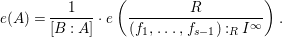 $$\begin{eqnarray}e(A)=\frac{1}{[B:A]}\cdot e\left(\frac{R}{(f_{1},\ldots ,f_{s-1}):_{R}I^{\infty }}\right).\end{eqnarray}$$
Proof. Let
 $f_{1},\ldots ,f_{s}$
be general
$f_{1},\ldots ,f_{s}$
be general
 $k$
-linear combinations of homogeneous minimal generators of
$k$
-linear combinations of homogeneous minimal generators of
 $I$
. Let
$I$
. Let
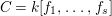 $C=k[f_{1},\ldots ,f_{s}]$
. Since
$C=k[f_{1},\ldots ,f_{s}]$
. Since
 $A$
has dimension
$A$
has dimension
 $s$
, the homogeneous ring extension
$s$
, the homogeneous ring extension
 $C\subset A$
is module-finite and
$C\subset A$
is module-finite and
 $C$
is a polynomial ring. Hence
$C$
is a polynomial ring. Hence
 $[A:C]=e(A)$
by Observation 2.8, for instance.
$[A:C]=e(A)$
by Observation 2.8, for instance.
We have the inclusion of domains
 $$\begin{eqnarray}C\subset A\subset B.\end{eqnarray}$$
We compute the field degree
 $[B:C]$
in two different ways. First,
$[B:C]$
in two different ways. First,
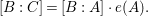 $$\begin{eqnarray}[B:C]=[B:A]\cdot e(A).\end{eqnarray}$$
Next, we wish to apply Proposition 3.6 to express
 $[B:C]$
. By the general choice of
$[B:C]$
. By the general choice of
 $f_{1},\ldots ,f_{s}$
, we may assume that
$f_{1},\ldots ,f_{s}$
, we may assume that
 $[0:\ldots :0:1]$
is a general point of
$[0:\ldots :0:1]$
is a general point of
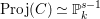 $\operatorname{Proj}(C)\simeq \mathbb{P}_{k}^{s-1}$
. The homogeneous prime ideal of
$\operatorname{Proj}(C)\simeq \mathbb{P}_{k}^{s-1}$
. The homogeneous prime ideal of
 $C$
corresponding to this point is
$C$
corresponding to this point is
 $\mathfrak{p}=(f_{1},\ldots ,f_{s-1})C$
. Therefore, Proposition 3.6 shows that
$\mathfrak{p}=(f_{1},\ldots ,f_{s-1})C$
. Therefore, Proposition 3.6 shows that
 $$\begin{eqnarray}[B:C]=e\left(\frac{R}{(f_{1},\ldots ,f_{s-1}):_{R}(f_{s})^{\infty }}\right).\end{eqnarray}$$
On the other hand,
 $$\begin{eqnarray}(f_{1},\ldots ,f_{s-1}):_{R}(f_{s})^{\infty }=(f_{1},\ldots ,f_{s-1}):_{R}I^{\infty }\end{eqnarray}$$
because
 $f_{s}$
is a general
$f_{s}$
is a general
 $k$
-linear combination of the homogeneous minimal generators of
$k$
-linear combination of the homogeneous minimal generators of
 $I$
. The proof is complete.◻
$I$
. The proof is complete.◻
We promised in the introduction to relate the degree of the rational map  of Data 3.1, the degree of the image, and the
 $j$
-multiplicity of the ideal
$j$
-multiplicity of the ideal
 $I$
. The relation is
$I$
. The relation is
 $$\begin{eqnarray}j(I)=d[B:A]e(A).\end{eqnarray}$$
A very quick proof of this formula is available in the present situation. Another proof of this formula, in a more general setting, is given in Theorem 5.3.
Corollary 3.8. Adopt the data of 3.1. Then
 $$\begin{eqnarray}j(I)=d[B:A]e(A).\end{eqnarray}$$
Proof. According to [Reference Xie53, 2.5] (see also [Reference Achilles and Manaresi1, 3.8] and [Reference Nishida and Ulrich42, 3.6])
 $$\begin{eqnarray}j(I)=\unicode[STIX]{x1D706}_{R}\left(\frac{R}{((f_{1},\ldots ,f_{s-1}):_{R}I^{\infty },f_{s})}\right),\end{eqnarray}$$
in the language of Corollary 3.7. On the other hand,
 $f_{s}$
is regular on
$f_{s}$
is regular on
 $R/(f_{1},\ldots ,f_{s-1}):_{R}I^{\infty }$
, and
$R/(f_{1},\ldots ,f_{s-1}):_{R}I^{\infty }$
, and
 $f_{s}$
is a homogeneous element of
$f_{s}$
is a homogeneous element of
 $R$
of degree
$R$
of degree
 $d$
; so,
$d$
; so,
 $$\begin{eqnarray}\unicode[STIX]{x1D706}_{R}\left(\frac{R}{((f_{1},\ldots ,f_{s-1}):_{R}I^{\infty },f_{s})}\right)=d\cdot e\left(\frac{R}{(f_{1},\ldots ,f_{s-1}):_{R}I^{\infty }}\right),\end{eqnarray}$$
and the assertion follows from Corollary 3.7. ◻
We now relate the fibers of the morphism
 $\unicode[STIX]{x1D6F9}$
of Data 3.1 to the generalized row ideals of the presentation matrix
$\unicode[STIX]{x1D6F9}$
of Data 3.1 to the generalized row ideals of the presentation matrix
 $\unicode[STIX]{x1D711}$
of
$\unicode[STIX]{x1D711}$
of
 $I$
. This material is taken from [Reference Eisenbud and Ulrich19]. For a point
$I$
. This material is taken from [Reference Eisenbud and Ulrich19]. For a point
 $p\in \mathbb{P}_{k}^{n-1}$
the ideal
$p\in \mathbb{P}_{k}^{n-1}$
the ideal
 $I_{1}(p\unicode[STIX]{x1D711})$
is well defined: one may use any representative of
$I_{1}(p\unicode[STIX]{x1D711})$
is well defined: one may use any representative of
 $p$
when computing the matrix product
$p$
when computing the matrix product
 $p\unicode[STIX]{x1D711}$
.
$p\unicode[STIX]{x1D711}$
.
Observation 3.9. Adopt Data 3.1. If
 $\mathfrak{P}$
is the homogeneous prime ideal in
$\mathfrak{P}$
is the homogeneous prime ideal in
 $S$
which corresponds to the rational point
$S$
which corresponds to the rational point
 $p$
in
$p$
in
 $\mathbb{P}_{k}^{n-1}$
, then the ideals
$\mathbb{P}_{k}^{n-1}$
, then the ideals
 $\mathfrak{P}R:I^{\infty }$
and
$\mathfrak{P}R:I^{\infty }$
and
 $I_{1}(p\unicode[STIX]{x1D711}):I^{\infty }$
of
$I_{1}(p\unicode[STIX]{x1D711}):I^{\infty }$
of
 $R$
are equal.
$R$
are equal.
Proof. Let
 $p=[\unicode[STIX]{x1D6FC}_{1}:\cdots :\unicode[STIX]{x1D6FC}_{n}]$
with
$p=[\unicode[STIX]{x1D6FC}_{1}:\cdots :\unicode[STIX]{x1D6FC}_{n}]$
with
 $\unicode[STIX]{x1D6FC}_{i}$
in
$\unicode[STIX]{x1D6FC}_{i}$
in
 $k$
. Recall the generating sets given in (3.4.1) and (3.4.2) for the ideals
$k$
. Recall the generating sets given in (3.4.1) and (3.4.2) for the ideals
 $\mathfrak{P}$
and
$\mathfrak{P}$
and
 $\mathfrak{P}R$
of
$\mathfrak{P}R$
of
 $S$
and
$S$
and
 $R$
, respectively. Let
$R$
, respectively. Let
 $\unicode[STIX]{x1D712}$
be an invertible matrix with entries in
$\unicode[STIX]{x1D712}$
be an invertible matrix with entries in
 $k$
and
$k$
and
 $(0,\ldots ,0,1)=(\unicode[STIX]{x1D6FC}_{1},\ldots ,\unicode[STIX]{x1D6FC}_{n})\unicode[STIX]{x1D712}$
. Define
$(0,\ldots ,0,1)=(\unicode[STIX]{x1D6FC}_{1},\ldots ,\unicode[STIX]{x1D6FC}_{n})\unicode[STIX]{x1D712}$
. Define
 $[g_{1}^{\prime },\ldots ,g_{n}^{\prime }]=\pmb{g}^{\prime }$
by
$[g_{1}^{\prime },\ldots ,g_{n}^{\prime }]=\pmb{g}^{\prime }$
by
 $$\begin{eqnarray}\pmb{g}^{\prime }=[g_{1},\ldots ,g_{n}]\unicode[STIX]{x1D712}.\end{eqnarray}$$
The entries of
 $\pmb{g}^{\prime }$
generate
$\pmb{g}^{\prime }$
generate
 $I$
and
$I$
and
 $\unicode[STIX]{x1D711}^{\prime }=\unicode[STIX]{x1D712}^{-1}\unicode[STIX]{x1D711}$
is a homogeneous syzygy matrix for
$\unicode[STIX]{x1D711}^{\prime }=\unicode[STIX]{x1D712}^{-1}\unicode[STIX]{x1D711}$
is a homogeneous syzygy matrix for
 $\pmb{g}^{\prime }$
. One consequence of this last statement is the fact that the bottom row of
$\pmb{g}^{\prime }$
. One consequence of this last statement is the fact that the bottom row of
 $\unicode[STIX]{x1D711}^{\prime }$
generates the ideal
$\unicode[STIX]{x1D711}^{\prime }$
generates the ideal
 $(g_{1}^{\prime },\ldots ,g_{n-1}^{\prime }):g_{n}^{\prime }$
. On the other hand,
$(g_{1}^{\prime },\ldots ,g_{n-1}^{\prime }):g_{n}^{\prime }$
. On the other hand,
 $$\begin{eqnarray}\left[\begin{array}{@{}ccc@{}}\unicode[STIX]{x1D6FC}_{1} & \ldots \, & \unicode[STIX]{x1D6FC}_{n}\\ g_{1} & \ldots \, & g_{n}\end{array}\right]\unicode[STIX]{x1D712}=\left[\begin{array}{@{}cccc@{}}0 & \ldots \, & 0 & 1\\ g_{1}^{\prime } & \ldots \, & g_{n-1}^{\prime } & g_{n}^{\prime }\end{array}\right];\end{eqnarray}$$
and the ideal of
 $2\times 2$
minors of a matrix is unchanged by row and column operations; therefore,
$2\times 2$
minors of a matrix is unchanged by row and column operations; therefore,
 $\mathfrak{P}R$
is generated by
$\mathfrak{P}R$
is generated by
 $(g_{1}^{\prime },\ldots ,g_{n-1}^{\prime })$
. We now see that
$(g_{1}^{\prime },\ldots ,g_{n-1}^{\prime })$
. We now see that
 $$\begin{eqnarray}I_{1}(p\unicode[STIX]{x1D711})=I_{1}([0,\ldots ,0,1]\unicode[STIX]{x1D711}^{\prime })=(g_{1}^{\prime },\ldots ,g_{n-1}^{\prime }):g_{n}^{\prime }=\mathfrak{P}R:I;\end{eqnarray}$$
hence,
 $I_{1}(p\unicode[STIX]{x1D711}):I^{\infty }=(\mathfrak{P}R:I):I^{\infty }=\mathfrak{P}R:I^{\infty }$
.◻
$I_{1}(p\unicode[STIX]{x1D711}):I^{\infty }=(\mathfrak{P}R:I):I^{\infty }=\mathfrak{P}R:I^{\infty }$
.◻
Recall that the degree of a subscheme of projective space is the multiplicity of its homogeneous coordinate ring.
Corollary 3.10. Adopt the data of 3.1. Let
 $p$
be a rational point in
$p$
be a rational point in
 $\mathbb{P}_{k}^{n-1}$
.
$\mathbb{P}_{k}^{n-1}$
.
-
(1) If
$k$
is algebraically closed, then
$p$
is in the image of
$\unicode[STIX]{x1D6F9}$
if and only if
$I_{1}(p\unicode[STIX]{x1D711}):I^{\infty }\neq R$
. -
(2) If
$p$
is in the image of
$\unicode[STIX]{x1D6F9}$
, then the degree of the fiber of
$\unicode[STIX]{x1D6F9}$
over
$p$
is equal to the multiplicity of
$R/(I_{1}(p\unicode[STIX]{x1D711}):I^{\infty })$
. -
(3) If the Krull dimension of
$A$
is equal to
$s$
and
$p=\unicode[STIX]{x1D6F9}(q)$
for
$q$
a general point in
$\mathbb{P}_{k}^{s-1}$
, then
$e(R/(I_{1}(p\unicode[STIX]{x1D711}):I^{\infty }))=[\operatorname{Quot}(B):\operatorname{Quot}(A)]$
.


Proof. For part (1) we use Observation 3.9, Remark 3.4(1) and the fact that the ideal
 $I_{1}(p\unicode[STIX]{x1D711}):I^{\infty }$
is not the unit ideal if and only it has dimension at least one. Item (2) follows from Observation 3.9. To prove item (3) we apply Observation 3.9 and Proposition 3.6.◻
$I_{1}(p\unicode[STIX]{x1D711}):I^{\infty }$
is not the unit ideal if and only it has dimension at least one. Item (2) follows from Observation 3.9. To prove item (3) we apply Observation 3.9 and Proposition 3.6.◻
More information about the rational map
 $\unicode[STIX]{x1D6F9}$
of Data 3.1 may be read from
$\unicode[STIX]{x1D6F9}$
of Data 3.1 may be read from
 $\unicode[STIX]{x1D711}$
when
$\unicode[STIX]{x1D711}$
when
 $I$
is an
$I$
is an
 $\mathfrak{m}$
-primary ideal. In this case,
$\mathfrak{m}$
-primary ideal. In this case,
 $\unicode[STIX]{x1D6F9}$
is actually a morphism and the image of
$\unicode[STIX]{x1D6F9}$
is actually a morphism and the image of
 $\unicode[STIX]{x1D6F9}$
is a closed subscheme of
$\unicode[STIX]{x1D6F9}$
is a closed subscheme of
 $\mathbb{P}_{k}^{n-1}$
. Even more information can be read when
$\mathbb{P}_{k}^{n-1}$
. Even more information can be read when
 $s=2$
. In this case the saturation of the row ideal
$s=2$
. In this case the saturation of the row ideal
 $I_{1}(p\unicode[STIX]{x1D711})$
is the ideal generated by the
$I_{1}(p\unicode[STIX]{x1D711})$
is the ideal generated by the
 $\text{gcd}$
of the entries of the product matrix
$\text{gcd}$
of the entries of the product matrix
 $p\unicode[STIX]{x1D711}$
and the image of
$p\unicode[STIX]{x1D711}$
and the image of
 $\unicode[STIX]{x1D6F9}$
is a curve
$\unicode[STIX]{x1D6F9}$
is a curve
 ${\mathcal{C}}$
.
${\mathcal{C}}$
.
Corollary 3.11. Adopt the data of 3.1. In addition assume that
 $I$
is
$I$
is
 $\mathfrak{m}$
-primary and
$\mathfrak{m}$
-primary and
 $s=2$
. Let
$s=2$
. Let
 ${\mathcal{C}}$
be the image of
${\mathcal{C}}$
be the image of
 $\unicode[STIX]{x1D6F9}$
. The following statements hold.
$\unicode[STIX]{x1D6F9}$
. The following statements hold.
-
(1) The point
$p$
is on the curve
${\mathcal{C}}$
if and only if
$\text{gcd}(I_{1}(p\unicode[STIX]{x1D711}))$
is not in
$k$
. -
(2) If
$p$
is on the curve
${\mathcal{C}}$
, then the multiplicity of the fiber of
$\unicode[STIX]{x1D6F9}$
over
$p$
is equal to
$$\begin{eqnarray}\deg (\text{gcd}(I_{1}(p\unicode[STIX]{x1D711}))).\end{eqnarray}$$
-
(3) If
$p=\unicode[STIX]{x1D6F9}(q)$
for
$q$
a general point in
$\mathbb{P}_{k}^{1}$
, then
$\deg (\text{gcd}(I_{1}(p\unicode[STIX]{x1D711})))=[\operatorname{Quot}(B):\operatorname{Quot}(A)]$
. -
(4) All entries of the matrix
$\unicode[STIX]{x1D711}$
have degree at least
$[\operatorname{Quot}(B):\operatorname{Quot}(A)]$
.


Proof. Items (1)–(3) follow from Corollary 3.10. As for item (4), notice that each column of
 $\unicode[STIX]{x1D711}$
contains a nonzero element, hence the linear space
$\unicode[STIX]{x1D711}$
contains a nonzero element, hence the linear space
 $$\begin{eqnarray}V=\{[\unicode[STIX]{x1D6FD}_{1},\ldots ,\unicode[STIX]{x1D6FD}_{n}]\in k^{n}\mid \sum \unicode[STIX]{x1D6FD}_{i}\unicode[STIX]{x1D711}_{ij}=0\}\end{eqnarray}$$
is a proper linear subspace of
 $\mathbb{P}_{k}^{n-1}$
. Because
$\mathbb{P}_{k}^{n-1}$
. Because
 $g_{1},\ldots ,g_{n}$
are
$g_{1},\ldots ,g_{n}$
are
 $k$
-linearly independent the image of
$k$
-linearly independent the image of
 $\unicode[STIX]{x1D6F9}$
cannot be contained in
$\unicode[STIX]{x1D6F9}$
cannot be contained in
 $V$
. Thus if
$V$
. Thus if
 $q$
is a general point in
$q$
is a general point in
 $\mathbb{P}_{k}^{1}$
every entry in the product
$\mathbb{P}_{k}^{1}$
every entry in the product
 $p\unicode[STIX]{x1D711}=\unicode[STIX]{x1D6F9}(q)\unicode[STIX]{x1D711}$
is nonzero. Now item (4) follows from (3).◻
$p\unicode[STIX]{x1D711}=\unicode[STIX]{x1D6F9}(q)\unicode[STIX]{x1D711}$
is nonzero. Now item (4) follows from (3).◻
4 Reparameterization
Data 4.1. (1) Let
 $R=k[x_{1},x_{2}]$
be a standard-graded polynomial ring over an infinite perfect field
$R=k[x_{1},x_{2}]$
be a standard-graded polynomial ring over an infinite perfect field
 $k$
with maximal homogeneous ideal
$k$
with maximal homogeneous ideal
 $\mathfrak{m}$
,
$\mathfrak{m}$
,
 $I$
be a height two ideal of
$I$
be a height two ideal of
 $R$
which is generated by homogeneous forms of the same degree
$R$
which is generated by homogeneous forms of the same degree
 $d$
,
$d$
,
 $A$
and
$A$
and
 $B$
be the
$B$
be the
 $k$
-subalgebras
$k$
-subalgebras
 $A=k[I_{d}]$
and
$A=k[I_{d}]$
and
 $B=k[R_{d}]$
of
$B=k[R_{d}]$
of
 $R$
, and
$R$
, and
 $r$
be the degree of the field extension
$r$
be the degree of the field extension
 $\operatorname{Quot}(A)\subset \operatorname{Quot}(B)$
. View
$\operatorname{Quot}(A)\subset \operatorname{Quot}(B)$
. View
 $A$
and
$A$
and
 $B$
as standard-graded
$B$
as standard-graded
 $k$
-algebras with maximal homogeneous ideals
$k$
-algebras with maximal homogeneous ideals
 $\mathfrak{m}_{A}$
and
$\mathfrak{m}_{A}$
and
 $\mathfrak{m}_{B}$
, respectively. Let
$\mathfrak{m}_{B}$
, respectively. Let
 $e=e(A)$
.
$e=e(A)$
.
(2) Let
 $g_{1},\ldots ,g_{n}$
be homogeneous forms in
$g_{1},\ldots ,g_{n}$
be homogeneous forms in
 $R$
of degree
$R$
of degree
 $d$
which minimally generate the ideal
$d$
which minimally generate the ideal
 $I$
and consider the morphism
$I$
and consider the morphism  which is defined by these forms; that is,
 $\unicode[STIX]{x1D6F9}$
sends the point
$\unicode[STIX]{x1D6F9}$
sends the point
 $q$
of
$q$
of
 $\mathbb{P}_{k}^{1}$
to the point
$\mathbb{P}_{k}^{1}$
to the point
 $[g_{1}(q):\cdots :g_{n}(q)]\in \mathbb{P}_{k}^{n-1}$
. The corresponding homomorphism of
$[g_{1}(q):\cdots :g_{n}(q)]\in \mathbb{P}_{k}^{n-1}$
. The corresponding homomorphism of
 $k$
-algebras is
$k$
-algebras is
 $\unicode[STIX]{x1D713}:S=k[T_{1},\ldots ,T_{n}]\rightarrow R$
, which sends
$\unicode[STIX]{x1D713}:S=k[T_{1},\ldots ,T_{n}]\rightarrow R$
, which sends
 $T_{i}$
to
$T_{i}$
to
 $g_{i}$
, for each
$g_{i}$
, for each
 $i$
.
$i$
.
(3) Let
 $\unicode[STIX]{x1D711}$
be a minimal homogeneous Hilbert–Burch matrix for the row vector
$\unicode[STIX]{x1D711}$
be a minimal homogeneous Hilbert–Burch matrix for the row vector
 $[g_{1},\ldots ,g_{n}]$
. In other words, there exist shifts
$[g_{1},\ldots ,g_{n}]$
. In other words, there exist shifts
 $D_{j}$
and a unit
$D_{j}$
and a unit
 $u$
in
$u$
in
 $k$
so that
$k$
so that

is a minimal homogeneous resolution of
 $R/I$
and
$R/I$
and
 $g_{i}$
is equal to
$g_{i}$
is equal to
 $u(-1)^{i}$
times the determinant of
$u(-1)^{i}$
times the determinant of
 $\unicode[STIX]{x1D711}$
with row
$\unicode[STIX]{x1D711}$
with row
 $i$
deleted, for
$i$
deleted, for
 $1\leqslant i\leqslant n$
.
$1\leqslant i\leqslant n$
.
In this section, we prove an algebraic analogue of a consequence of Hurwitz’ theorem. Let
 $r$
be the degree of the morphism
$r$
be the degree of the morphism  which at the level of coordinate rings corresponds to the embedding
 $A{\hookrightarrow}k[R_{d}]$
. Thus
$A{\hookrightarrow}k[R_{d}]$
. Thus
 $r$
is the degree of the field extension
$r$
is the degree of the field extension
 $\text{Quot}(A)\subset \text{Quot}(k[R_{d}])$
. We show that there exist homogeneous forms
$\text{Quot}(A)\subset \text{Quot}(k[R_{d}])$
. We show that there exist homogeneous forms
 $f_{1},f_{2}$
of degree
$f_{1},f_{2}$
of degree
 $r$
in
$r$
in
 $R$
such that the entries of the matrix
$R$
such that the entries of the matrix
 $\unicode[STIX]{x1D711}$
are homogeneous polynomials in the variables
$\unicode[STIX]{x1D711}$
are homogeneous polynomials in the variables
 $f_{1}$
and
$f_{1}$
and
 $f_{2}$
. In particular, the ideal
$f_{2}$
. In particular, the ideal
 $I$
is extended from an ideal in
$I$
is extended from an ideal in
 $k[f_{1},f_{2}]$
. Thus, replacing
$k[f_{1},f_{2}]$
. Thus, replacing
 $k[x_{1},x_{2}]$
by
$k[x_{1},x_{2}]$
by
 $k[f_{1},f_{2}]$
, we can reduce the nonbirational case to the birational one. Furthermore, we provide an explicit description of
$k[f_{1},f_{2}]$
, we can reduce the nonbirational case to the birational one. Furthermore, we provide an explicit description of
 $f_{1}$
and
$f_{1}$
and
 $f_{2}$
in terms of
$f_{2}$
in terms of
 $\unicode[STIX]{x1D711}$
. If
$\unicode[STIX]{x1D711}$
. If
 $q_{1}$
and
$q_{1}$
and
 $q_{2}$
are general points in
$q_{2}$
are general points in
 $\mathbb{P}_{k}^{1}$
, then
$\mathbb{P}_{k}^{1}$
, then
 $f_{i}=\text{gcd}(I_{1}(p_{i}\unicode[STIX]{x1D711}))$
with
$f_{i}=\text{gcd}(I_{1}(p_{i}\unicode[STIX]{x1D711}))$
with
 $p_{i}=\unicode[STIX]{x1D6F9}(q_{i})$
.
$p_{i}=\unicode[STIX]{x1D6F9}(q_{i})$
.
The first half of the present section is devoted to the proof of the main result, Theorem 4.2. In the second half of the section, beginning with Corollary 4.5, we use Theorem 4.2 to reduce the general (that is, nonbirational) case to the birational one.
Theorem 4.2. Adopt the data of 4.1. If
 $q_{1}$
and
$q_{1}$
and
 $q_{2}$
are general points in
$q_{2}$
are general points in
 $\mathbb{P}_{k}^{1}$
, then
$\mathbb{P}_{k}^{1}$
, then
 $A\subset k[f_{1},f_{2}]$
, where
$A\subset k[f_{1},f_{2}]$
, where
 $f_{i}=\text{gcd}(I_{1}(p_{i}\unicode[STIX]{x1D711}))$
with
$f_{i}=\text{gcd}(I_{1}(p_{i}\unicode[STIX]{x1D711}))$
with
 $p_{i}=\unicode[STIX]{x1D6F9}(q_{i})$
.
$p_{i}=\unicode[STIX]{x1D6F9}(q_{i})$
.
The proof of Theorem 4.2 involves a number of steps. Before getting started we record some numerical information. In preparation for the first step in the proof of Theorem 4.2, we record a result from [Reference Kustin, Polini and Ulrich36, Corollary 5.2]. Recall that a standard-graded Cohen–Macaulay
 $k$
-algebra
$k$
-algebra
 $C$
over a field
$C$
over a field
 $k$
with homogeneous maximal ideal
$k$
with homogeneous maximal ideal
 $\mathfrak{m}_{C}$
is said to have minimal multiplicity if its multiplicity has the smallest possible value, namely,
$\mathfrak{m}_{C}$
is said to have minimal multiplicity if its multiplicity has the smallest possible value, namely,
 $e(C)=\unicode[STIX]{x1D707}(\mathfrak{m}_{C})-\text{dim}(C)+1$
.
$e(C)=\unicode[STIX]{x1D707}(\mathfrak{m}_{C})-\text{dim}(C)+1$
.
Proposition 4.3. Let
 $k$
be a perfect field and
$k$
be a perfect field and
 $A\subset B$
a homogeneous integral extension of standard-graded
$A\subset B$
a homogeneous integral extension of standard-graded
 $k$
-domains. Further assume that
$k$
-domains. Further assume that
 $A$
is normal and Cohen–Macaulay. If
$A$
is normal and Cohen–Macaulay. If
 $B$
has minimal multiplicity, then so does
$B$
has minimal multiplicity, then so does
 $A$
.
$A$
.

Proof. Apply Proposition 4.3. In the present situation,
 $A$
and
$A$
and
 $B$
are normal of dimension
$B$
are normal of dimension
 $2$
and therefore Cohen–Macaulay, and
$2$
and therefore Cohen–Macaulay, and
 $B$
has minimal multiplicity since
$B$
has minimal multiplicity since
 $d=e(B)=\unicode[STIX]{x1D707}(\mathfrak{m}_{B})-1$
. It follows that
$d=e(B)=\unicode[STIX]{x1D707}(\mathfrak{m}_{B})-1$
. It follows that
 $A$
has minimal multiplicity as well, namely,
$A$
has minimal multiplicity as well, namely,
 $$\begin{eqnarray}e=\unicode[STIX]{x1D707}(\mathfrak{m}_{A})-1=\unicode[STIX]{x1D707}(I)-1=n-1.\end{eqnarray}$$
We conclude that the syzygy matrix
 $\unicode[STIX]{x1D711}$
has size
$\unicode[STIX]{x1D711}$
has size
 $e+1\times e$
. Each entry in column
$e+1\times e$
. Each entry in column
 $j$
of
$j$
of
 $\unicode[STIX]{x1D711}$
is a form of degree
$\unicode[STIX]{x1D711}$
is a form of degree
 $D_{j}$
, in the language of (4.1.1), and, according to Corollary 3.11(4),
$D_{j}$
, in the language of (4.1.1), and, according to Corollary 3.11(4),
 $D_{j}\geqslant r$
. The
$D_{j}\geqslant r$
. The
 $g_{i}$
have degree
$g_{i}$
have degree
 $d$
and each one of them is the determinant of an
$d$
and each one of them is the determinant of an
 $e\times e$
minor of
$e\times e$
minor of
 $\unicode[STIX]{x1D711}$
; thus,
$\unicode[STIX]{x1D711}$
; thus,
 $d=\sum _{j=1}^{e}D_{j}\geqslant er=d$
, where the last equality follows from Observation 3.2. We conclude that each entry of
$d=\sum _{j=1}^{e}D_{j}\geqslant er=d$
, where the last equality follows from Observation 3.2. We conclude that each entry of
 $\unicode[STIX]{x1D711}$
is a homogeneous form of degree
$\unicode[STIX]{x1D711}$
is a homogeneous form of degree
 $r$
.
$r$
.
Let
 $q_{1},\ldots ,q_{e+1}$
be general points in
$q_{1},\ldots ,q_{e+1}$
be general points in
 $\mathbb{P}_{k}^{1}$
. Hence the points
$\mathbb{P}_{k}^{1}$
. Hence the points
 $\unicode[STIX]{x1D6F9}(q_{1}),\ldots ,\unicode[STIX]{x1D6F9}(q_{e+1})$
are general on the curve
$\unicode[STIX]{x1D6F9}(q_{1}),\ldots ,\unicode[STIX]{x1D6F9}(q_{e+1})$
are general on the curve
 ${\mathcal{C}}=\text{Im}\,\unicode[STIX]{x1D6F9}$
, and since
${\mathcal{C}}=\text{Im}\,\unicode[STIX]{x1D6F9}$
, and since
 ${\mathcal{C}}$
is nondegenerate in
${\mathcal{C}}$
is nondegenerate in
 $\mathbb{P}^{e}$
, it follows that
$\mathbb{P}^{e}$
, it follows that
 $\unicode[STIX]{x1D6F9}(q_{1}),\ldots ,\unicode[STIX]{x1D6F9}(q_{e+1})$
span
$\unicode[STIX]{x1D6F9}(q_{1}),\ldots ,\unicode[STIX]{x1D6F9}(q_{e+1})$
span
 $\mathbb{P}^{e}$
. In other words, the
$\mathbb{P}^{e}$
. In other words, the
 $(e+1)\times (e+1)$
scalar matrix
$(e+1)\times (e+1)$
scalar matrix
 $\unicode[STIX]{x1D6E4}$
, whose rows are
$\unicode[STIX]{x1D6E4}$
, whose rows are
 $\unicode[STIX]{x1D6F9}(q_{i})$
, is invertible. We apply Corollary 3.11(3) to see that each
$\unicode[STIX]{x1D6F9}(q_{i})$
, is invertible. We apply Corollary 3.11(3) to see that each
 $\text{gcd}(I_{1}(\unicode[STIX]{x1D6F9}(q_{i})\unicode[STIX]{x1D711}))$
is a form in
$\text{gcd}(I_{1}(\unicode[STIX]{x1D6F9}(q_{i})\unicode[STIX]{x1D711}))$
is a form in
 $R$
of degree
$R$
of degree
 $r$
. Write
$r$
. Write
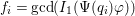 $f_{i}=\text{gcd}(I_{1}(\unicode[STIX]{x1D6F9}(q_{i})\unicode[STIX]{x1D711}))$
. Degree considerations show that
$f_{i}=\text{gcd}(I_{1}(\unicode[STIX]{x1D6F9}(q_{i})\unicode[STIX]{x1D711}))$
. Degree considerations show that
 $$\begin{eqnarray}\unicode[STIX]{x1D6F9}(q_{i})\unicode[STIX]{x1D711}=f_{i}\cdot \unicode[STIX]{x1D706}_{i},\end{eqnarray}$$
where
 $\unicode[STIX]{x1D706}_{i}$
is a vector of scalars. It follows that
$\unicode[STIX]{x1D706}_{i}$
is a vector of scalars. It follows that
 $$\begin{eqnarray}\unicode[STIX]{x1D6E4}\unicode[STIX]{x1D711}=D\unicode[STIX]{x1D6EC},\end{eqnarray}$$
where
 $D$
is the diagonal matrix whose diagonal entries are the forms
$D$
is the diagonal matrix whose diagonal entries are the forms
 $f_{1},\ldots ,f_{e+1}$
, and
$f_{1},\ldots ,f_{e+1}$
, and
 $\unicode[STIX]{x1D6EC}$
is the
$\unicode[STIX]{x1D6EC}$
is the
 $(e+1)\times e$
scalar matrix whose rows are the
$(e+1)\times e$
scalar matrix whose rows are the
 $\unicode[STIX]{x1D706}_{i}$
. We notice that
$\unicode[STIX]{x1D706}_{i}$
. We notice that
 $\unicode[STIX]{x1D6EC}$
has maximal rank
$\unicode[STIX]{x1D6EC}$
has maximal rank
 $e$
because
$e$
because
 $\unicode[STIX]{x1D711}$
does.
$\unicode[STIX]{x1D711}$
does.
Let
 $q$
be another general point in
$q$
be another general point in
 $\mathbb{P}^{1}$
. Write
$\mathbb{P}^{1}$
. Write
 $$\begin{eqnarray}\unicode[STIX]{x1D6F9}(q)\unicode[STIX]{x1D711}=f\unicode[STIX]{x1D706},\end{eqnarray}$$
as in (4.4.1), where
 $f$
is a form of degree
$f$
is a form of degree
 $r$
in
$r$
in
 $R$
and
$R$
and
 $\unicode[STIX]{x1D706}$
is a row vector of scalars from
$\unicode[STIX]{x1D706}$
is a row vector of scalars from
 $k$
. There is an
$k$
. There is an
 $e\times (e-1)$
matrix of scalars
$e\times (e-1)$
matrix of scalars
 $\unicode[STIX]{x1D6E5}$
so that
$\unicode[STIX]{x1D6E5}$
so that
 $\unicode[STIX]{x1D706}\unicode[STIX]{x1D6E5}=0$
and
$\unicode[STIX]{x1D706}\unicode[STIX]{x1D6E5}=0$
and
 $\unicode[STIX]{x1D6E5}$
has full rank
$\unicode[STIX]{x1D6E5}$
has full rank
 $e-1$
. Combine (4.4.3), the definition of
$e-1$
. Combine (4.4.3), the definition of
 $\unicode[STIX]{x1D6F9}$
as given in 4.1(2), and (4.4.2) to see that
$\unicode[STIX]{x1D6F9}$
as given in 4.1(2), and (4.4.2) to see that
 $$\begin{eqnarray}0=f\unicode[STIX]{x1D706}\unicode[STIX]{x1D6E5}=\unicode[STIX]{x1D6F9}(q)\unicode[STIX]{x1D711}\unicode[STIX]{x1D6E5}=[g_{1}(q),\ldots ,g_{e+1}(q)]\unicode[STIX]{x1D6E4}^{-1}D\unicode[STIX]{x1D6EC}\unicode[STIX]{x1D6E5}.\end{eqnarray}$$
The point
 $q$
in
$q$
in
 $\mathbb{P}^{1}$
is general; so the product
$\mathbb{P}^{1}$
is general; so the product
 $[g_{1}(q),\ldots ,g_{e+1}(q)]\unicode[STIX]{x1D6E4}^{-1}$
is a row vector of nonzero scalars and the product
$[g_{1}(q),\ldots ,g_{e+1}(q)]\unicode[STIX]{x1D6E4}^{-1}$
is a row vector of nonzero scalars and the product
 $[g_{1}(q),\ldots ,g_{e+1}(q)]\unicode[STIX]{x1D6E4}^{-1}D$
is equal to
$[g_{1}(q),\ldots ,g_{e+1}(q)]\unicode[STIX]{x1D6E4}^{-1}D$
is equal to
 $[f_{1},\ldots ,f_{e+1}]D^{\prime }$
, where
$[f_{1},\ldots ,f_{e+1}]D^{\prime }$
, where
 $D^{\prime }$
is an invertible diagonal matrix of scalars. Thus,
$D^{\prime }$
is an invertible diagonal matrix of scalars. Thus,
 $$\begin{eqnarray}0=[f_{1},\ldots ,f_{e+1}]D^{\prime }\unicode[STIX]{x1D6EC}\unicode[STIX]{x1D6E5},\end{eqnarray}$$
where
 $D^{\prime }\unicode[STIX]{x1D6EC}\unicode[STIX]{x1D6E5}$
is an
$D^{\prime }\unicode[STIX]{x1D6EC}\unicode[STIX]{x1D6E5}$
is an
 $(e+1)\times (e-1)$
matrix of scalars of rank
$(e+1)\times (e-1)$
matrix of scalars of rank
 $e-1$
. We conclude that the vector space
$e-1$
. We conclude that the vector space
 $V$
spanned by the homogeneous forms
$V$
spanned by the homogeneous forms
 $f_{1},\ldots ,f_{e+1}$
has dimension at most two. Select a generating set
$f_{1},\ldots ,f_{e+1}$
has dimension at most two. Select a generating set
 $f_{i},f_{j}$
for
$f_{i},f_{j}$
for
 $V$
. Every entry of the Hilbert–Burch matrix
$V$
. Every entry of the Hilbert–Burch matrix
 $\unicode[STIX]{x1D711}$
is an element of the ring
$\unicode[STIX]{x1D711}$
is an element of the ring
 $k[f_{i},f_{j}]$
(as can be seen from (4.4.2)); hence
$k[f_{i},f_{j}]$
(as can be seen from (4.4.2)); hence
 $A=k[I_{d}]\subset k[f_{i},f_{j}]$
and the proof of Claim 4.4 is complete.◻
$A=k[I_{d}]\subset k[f_{i},f_{j}]$
and the proof of Claim 4.4 is complete.◻
Next we are ready to prove Theorem 4.2.
Proof. We prove the theorem by reducing to the normal case. The integral closure
 $\overline{A}$
of
$\overline{A}$
of
 $A$
in
$A$
in
 $\operatorname{Quot}(A)$
is a graded
$\operatorname{Quot}(A)$
is a graded
 $k$
-subalgebra of
$k$
-subalgebra of
 $B$
, though not necessarily standard-graded. However,
$B$
, though not necessarily standard-graded. However,
 $\overline{A}$
is a finitely generated graded module over the standard-graded
$\overline{A}$
is a finitely generated graded module over the standard-graded
 $k$
-algebra
$k$
-algebra
 $A$
and hence there exists a positive integer
$A$
and hence there exists a positive integer
 $s$
such that the
$s$
such that the
 $t$
-Veronese subring of the integral closure of
$t$
-Veronese subring of the integral closure of
 $A$
, denoted
$A$
, denoted
 $\overline{A}^{(t)}$
, is standard-graded for all
$\overline{A}^{(t)}$
, is standard-graded for all
 $t\geqslant s$
. We observe that
$t\geqslant s$
. We observe that
 $\overline{A}^{(t)}=\overline{A^{(t)}}$
.
$\overline{A}^{(t)}=\overline{A^{(t)}}$
.
We apply Claim 4.4 to
 $\overline{A^{(s)}}$
. For general points
$\overline{A^{(s)}}$
. For general points
 $q_{1}$
and
$q_{1}$
and
 $q_{2}$
in
$q_{2}$
in
 $\mathbb{P}_{k}^{1}$
we obtain forms
$\mathbb{P}_{k}^{1}$
we obtain forms
 $\widetilde{f_{1}}$
and
$\widetilde{f_{1}}$
and
 $\widetilde{f_{2}}$
such that
$\widetilde{f_{2}}$
such that
 $\overline{A^{(s)}}\subset k[\widetilde{f_{1}},\widetilde{f_{2}}]$
. Let
$\overline{A^{(s)}}\subset k[\widetilde{f_{1}},\widetilde{f_{2}}]$
. Let
 $\mathfrak{Q_{i}}$
be the prime ideals in
$\mathfrak{Q_{i}}$
be the prime ideals in
 $R$
corresponding to
$R$
corresponding to
 $q_{i}$
. We have
$q_{i}$
. We have
 $$\begin{eqnarray}\displaystyle \widetilde{f_{i}}R & = & \displaystyle ((\mathfrak{Q_{i}}\cap \overline{A^{(s)}})R):\mathfrak{m}^{\infty }\nonumber\\ \displaystyle & = & \displaystyle ((\mathfrak{Q_{i}}\cap A^{(s)})R):\mathfrak{m}^{\infty }=((\mathfrak{Q_{i}}\cap A)R):\mathfrak{m}^{\infty }=f_{i}R,\nonumber\end{eqnarray}$$
where the first and last equality follow from Observation 3.9 (and 2.1) and the second and third equality hold due to Remark 3.5. We conclude that
 $\widetilde{f_{i}}k=f_{i}k$
and therefore
$\widetilde{f_{i}}k=f_{i}k$
and therefore
 $\overline{A^{(s)}}\subset k[f_{1},f_{2}]$
. In the same manner we obtain
$\overline{A^{(s)}}\subset k[f_{1},f_{2}]$
. In the same manner we obtain
 $\overline{A^{(s+1)}}\subset k[f_{1},f_{2}]$
. Hence for every nonzero homogeneous element
$\overline{A^{(s+1)}}\subset k[f_{1},f_{2}]$
. Hence for every nonzero homogeneous element
 $\unicode[STIX]{x1D6FC}$
in
$\unicode[STIX]{x1D6FC}$
in
 $A$
we have
$A$
we have
 $$\begin{eqnarray}\unicode[STIX]{x1D6FC}=\frac{\unicode[STIX]{x1D6FC}^{s+1}}{\unicode[STIX]{x1D6FC}^{s}}\in \text{Quot}(k[f_{1},f_{2}]).\end{eqnarray}$$
On the other hand,
 $\unicode[STIX]{x1D6FC}$
is integral over
$\unicode[STIX]{x1D6FC}$
is integral over
 $A^{(s)}$
, hence integral over
$A^{(s)}$
, hence integral over
 $k[f_{1},f_{2}]$
. We conclude that
$k[f_{1},f_{2}]$
. We conclude that
 $\unicode[STIX]{x1D6FC}\in k[f_{1},f_{2}]$
since
$\unicode[STIX]{x1D6FC}\in k[f_{1},f_{2}]$
since
 $k[f_{1},f_{2}]$
is normal.◻
$k[f_{1},f_{2}]$
is normal.◻
Corollary 4.5. Adopt the data of 4.1. Let
 $f_{1}$
and
$f_{1}$
and
 $f_{2}$
as in Theorem 4.2.
$f_{2}$
as in Theorem 4.2.
-
(1) The elements
$f_{1}$
,
$f_{2}$
are a regular sequence of forms of degree
$r$
in
$R$
. -
(2) The ring
$R^{\prime }=k[f_{1},f_{2}]$
is a polynomial ring in the variables
$f_{1}$
and
$f_{2}$
. After regrading, we view
$R^{\prime }$
as a standard-graded
$k$
-algebra. -
(3) The vector space
$I_{d}$
is a subset of
$R^{\prime }$
and the ideal
$I^{\prime }=I_{d}R^{\prime }$
is generated by forms of degree
$d/r$
in
$R^{\prime }$
. -
(4) The extension
$A=k[I_{d/r}^{\prime }]\subset k[R_{d/r}^{\prime }]$
is birational. -
(5) The ring
$R$
is a free
$R^{\prime }$
-module of rank
$r^{2}$
and
$I=I^{\prime }R$
. -
(6) There exists a minimal homogeneous Hilbert–Burch matrix for the row vector
$[g_{1},\ldots ,g_{n}]$
whose entries are in the ring
$k[f_{1},f_{2}]$
.


Proof. The forms
 $f_{1}$
and
$f_{1}$
and
 $f_{2}$
have degree
$f_{2}$
have degree
 $r$
according to Corollary 3.11(3). From Theorem 4.2 we obtain
$r$
according to Corollary 3.11(3). From Theorem 4.2 we obtain
 $I_{d}\subset R^{\prime }=k[f_{1},f_{2}]$
. In particular,
$I_{d}\subset R^{\prime }=k[f_{1},f_{2}]$
. In particular,
 $I\subset (f_{1},f_{2})R$
because
$I\subset (f_{1},f_{2})R$
because
 $I=I_{d}R$
. It follows that
$I=I_{d}R$
. It follows that
 $f_{1}$
,
$f_{1}$
,
 $f_{2}$
form a regular sequence in
$f_{2}$
form a regular sequence in
 $R$
and hence
$R$
and hence
 $R$
is a free module over
$R$
is a free module over
 $R^{\prime }=k[f_{1},f_{2}]$
, necessarily of rank
$R^{\prime }=k[f_{1},f_{2}]$
, necessarily of rank
 $r^{2}$
. Parts (1) and (5) are established. At this point, items (2), (3), and (6) are clear.
$r^{2}$
. Parts (1) and (5) are established. At this point, items (2), (3), and (6) are clear.
To prove (4) we use the following diagram, where the relevant field degrees are displayed:
The diagram shows
 $[k[R_{d/r}^{\prime }]:A]=1$
.◻
$[k[R_{d/r}^{\prime }]:A]=1$
.◻
In the following corollary we gather important numerical consequences of Theorem 4.2.
Corollary 4.6. Adopt the data of 4.1.
-
(1)
$[B:A]\mid \text{deg}[\unicode[STIX]{x1D711}]_{ij}$
. -
(2)
$[B:A]\mid \text{gcd}(\mathit{column~degrees~of}\;\unicode[STIX]{x1D711})$
. -
(3) If
$\text{gcd}(\mathit{column~degrees~of}\;\unicode[STIX]{x1D711})=1$
, then
$A\subset B$
is a birational extension; in other words,
$\unicode[STIX]{x1D6F9}$
is birational onto its image. -
(4) If every entry of
$\unicode[STIX]{x1D711}$
has the same degree and that degree is a prime integer, then the morphism
$\unicode[STIX]{x1D6F9}$
is birational onto its image if and only if
$\unicode[STIX]{x1D707}(I_{1}(\unicode[STIX]{x1D711}))\geqslant 3$
.


Proof. Items (1) and (2) follow from items (1)–(6) of Corollary 4.5. Item (3) is now clear. Item (4) is [Reference Cox, Kustin, Polini and Ulrich16, 0.11]. ◻
Observation 4.7. Adopt the data of 4.1 and assume that
 $I$
is a monomial ideal. Then
$I$
is a monomial ideal. Then
 $$\begin{eqnarray}[B:A]=\text{gcd}(\text{column degrees of }\unicode[STIX]{x1D711}).\end{eqnarray}$$
Proof. We may assume that
 $g_{i}=x^{a_{i}}y^{d-a_{i}}$
with
$g_{i}=x^{a_{i}}y^{d-a_{i}}$
with
 $0=a_{1}<a_{2}<\cdots <a_{n}=d$
. Hence in the language of (4.1.1),
$0=a_{1}<a_{2}<\cdots <a_{n}=d$
. Hence in the language of (4.1.1),
 $$\begin{eqnarray}D_{j}=a_{j+1}-a_{j}\quad \text{for }1\leqslant j\leqslant n-1.\end{eqnarray}$$
On the other hand, as is well known,
 $$\begin{eqnarray}[R:A]\mathbb{Z}=I_{2}\left(\begin{array}{@{}cccc@{}}a_{1} & a_{2} & \ldots & a_{n}\\ d-a_{1} & d-a_{2} & \ldots & d-a_{n}\end{array}\right).\end{eqnarray}$$
After row and column operations on the matrix, this determinantal ideal becomes
 $$\begin{eqnarray}d\cdot I_{2}\left(\begin{array}{@{}cccc@{}}0 & a_{2}-a_{1} & \ldots & a_{n}-a_{n-1}\\ 1 & 0 & \ldots & 0\end{array}\right)=d\cdot \text{gcd}(D_{1},\ldots ,D_{n-1})\mathbb{Z}.\end{eqnarray}$$
It follows that
 $$\begin{eqnarray}[B:A]=\frac{[R:A]}{d}=\text{gcd}(D_{1},\ldots ,D_{n-1})=\text{gcd}(\text{column degrees of }\unicode[STIX]{x1D711}).\square\end{eqnarray}$$
Remark 4.8. Adopt the data of 4.1. If
 $I$
is a monomial ideal
$I$
is a monomial ideal
 $$\begin{eqnarray}\text{gcd}(\text{column degrees of }\unicode[STIX]{x1D711})=1\;\Longleftrightarrow \;A\subset B\text{ is a birational extension}.\end{eqnarray}$$
However, the direction
 $(\Leftarrow )$
is far from true if the ideal
$(\Leftarrow )$
is far from true if the ideal
 $I$
is not monomial; see, for example, Corollary 4.6(4) or all of [Reference Cox, Kustin, Polini and Ulrich16].
$I$
is not monomial; see, for example, Corollary 4.6(4) or all of [Reference Cox, Kustin, Polini and Ulrich16].
The following theorem summarizes some of the results of the present section that were used in [Reference Cox, Kustin, Polini and Ulrich16]. It was recorded as [Reference Cox, Kustin, Polini and Ulrich16, Theorem 0.10]. (The present statement is the correct one.)
Theorem 4.9. Let
 $R$
be the standard-graded polynomial ring
$R$
be the standard-graded polynomial ring
 $k[x,y]$
, with
$k[x,y]$
, with
 $k$
an infinite perfect field,
$k$
an infinite perfect field,
 $I$
be a height two ideal of
$I$
be a height two ideal of
 $R$
generated by forms
$R$
generated by forms
 $g_{1},\ldots ,g_{n}$
of degree
$g_{1},\ldots ,g_{n}$
of degree
 $d$
, and
$d$
, and
 $\unicode[STIX]{x1D711}$
be a homogeneous Hilbert–Burch matrix for the row vector
$\unicode[STIX]{x1D711}$
be a homogeneous Hilbert–Burch matrix for the row vector
 $[g_{1},\ldots ,g_{n}]$
. If
$[g_{1},\ldots ,g_{n}]$
. If
 $A$
and
$A$
and
 $B$
are the standard-graded
$B$
are the standard-graded
 $k$
-algebras
$k$
-algebras
 $A=k[I_{d}]$
and
$A=k[I_{d}]$
and
 $B=k[R_{d}]$
,
$B=k[R_{d}]$
,
 $r$
is the degree of the field extension
$r$
is the degree of the field extension
 $[\operatorname{Quot}(B):\operatorname{Quot}(A)]$
, and
$[\operatorname{Quot}(B):\operatorname{Quot}(A)]$
, and
 $e$
is the multiplicity of
$e$
is the multiplicity of
 $A$
, then the following statements hold.
$A$
, then the following statements hold.
-
(1)
$re=d$
. -
(2) The morphism
$\mathbb{P}_{k}^{1}\rightarrow \mathbb{P}_{k}^{n-1}$
, which is given by
$q\mapsto [g_{1}(q):\cdots :g_{n}(q)]$
, is birational onto its image if and only if
$e=d$
. -
(3) There exist forms
$f_{1}$
and
$f_{2}$
of degree
$r$
in
$R$
such that
$A\subset k[f_{1},f_{2}]$
. In particular,
$I$
is extended from an ideal in
$k[f_{1},f_{2}]$
in the sense that
$I=(I\cap k[f_{1},f_{2}])R$
. Furthermore, we can choose
$f_{i}=\gcd (I_{1}(p_{i}\unicode[STIX]{x1D711}))$
where
$p_{i}=[g_{1}(q_{i}):\cdots :g_{n}(q_{i})]$
for general points
$q_{1}$
and
$q_{2}$
in
$\mathbb{P}_{k}^{1}$
.


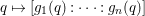


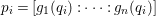


5 Rees rings
Data 5.1. Let
 $R$
be a standard-graded domain over a field
$R$
be a standard-graded domain over a field
 $k$
, of dimension
$k$
, of dimension
 $s$
, with maximal homogeneous ideal
$s$
, with maximal homogeneous ideal
 $\mathfrak{m}$
. Let
$\mathfrak{m}$
. Let
 $I$
be a homogeneous ideal in
$I$
be a homogeneous ideal in
 $R$
generated by forms of degree
$R$
generated by forms of degree
 $d$
,
$d$
,
 $A$
be the ring
$A$
be the ring
 $k[I_{d}]$
, and
$k[I_{d}]$
, and
 $B$
be the Veronese ring
$B$
be the Veronese ring
 $k[R_{d}]$
. After regrading, we view
$k[R_{d}]$
. After regrading, we view
 $A\subset B$
as standard-graded
$A\subset B$
as standard-graded
 $k$
-algebras.
$k$
-algebras.
In this section, we relate properties of the extension
 $A\subset B$
to properties of the corresponding inclusions of Rees algebras
$A\subset B$
to properties of the corresponding inclusions of Rees algebras
 ${\mathcal{R}}(I)\subset {\mathcal{R}}(\mathfrak{m}^{d})$
. The extension of Rees algebras has the advantage that it is automatically birational.
${\mathcal{R}}(I)\subset {\mathcal{R}}(\mathfrak{m}^{d})$
. The extension of Rees algebras has the advantage that it is automatically birational.
Remark 5.2. Adopt the data of 5.1. The injective map of graded
 $k$
-algebras
$k$
-algebras
 $$\begin{eqnarray}A\cong k[I_{d}t]{\hookrightarrow}R[It]={\mathcal{R}}(I)\end{eqnarray}$$
induces an isomorphism between the ring
 $A$
and the special fiber ring
$A$
and the special fiber ring
 ${\mathcal{R}}(I)/\mathfrak{m}{\mathcal{R}}(I)$
; see, for example, (2.12). The ring
${\mathcal{R}}(I)/\mathfrak{m}{\mathcal{R}}(I)$
; see, for example, (2.12). The ring
 $A$
is a domain; hence,
$A$
is a domain; hence,
 $\mathfrak{m}{\mathcal{R}}(I)$
is a prime ideal. Since
$\mathfrak{m}{\mathcal{R}}(I)$
is a prime ideal. Since
 $\text{dim}\,{\mathcal{R}}(I)$
is equal to
$\text{dim}\,{\mathcal{R}}(I)$
is equal to
 $s+1$
(see, for example, [Reference Swanson and Huneke51, 5.1.4]), we obtain
$s+1$
(see, for example, [Reference Swanson and Huneke51, 5.1.4]), we obtain
 $$\begin{eqnarray}\text{dim}\,A=s+1-\text{dim}\,{\mathcal{R}}(I)_{\mathfrak{m}{\mathcal{R}}(I)}.\end{eqnarray}$$
In the next result we show that the degree of the morphism
 $\unicode[STIX]{x1D6F9}:\mathbb{P}_{k}^{s-1}\longrightarrow \text{Im}\,\unicode[STIX]{x1D6F9}$
is equal to the multiplicity of the local ring
$\unicode[STIX]{x1D6F9}:\mathbb{P}_{k}^{s-1}\longrightarrow \text{Im}\,\unicode[STIX]{x1D6F9}$
is equal to the multiplicity of the local ring
 ${\mathcal{R}}(I)_{\mathfrak{m}{\mathcal{R}}(I)}$
. In addition, we relate the degree of the morphism
${\mathcal{R}}(I)_{\mathfrak{m}{\mathcal{R}}(I)}$
. In addition, we relate the degree of the morphism
 $\unicode[STIX]{x1D6F9}$
, the degree of the image, and the
$\unicode[STIX]{x1D6F9}$
, the degree of the image, and the
 $j$
-multiplicity of the ideal
$j$
-multiplicity of the ideal
 $I$
. The notion of
$I$
. The notion of
 $j$
-multiplicity and the importance of this result is discussed in the introduction and in Corollary 3.8.
$j$
-multiplicity and the importance of this result is discussed in the introduction and in Corollary 3.8.
Theorem 5.3. Adopt the data of 5.1. If the Krull dimension of
 $A$
is equal to
$A$
is equal to
 $s$
, then
$s$
, then
 $$\begin{eqnarray}e({\mathcal{R}}(I)_{\mathfrak{m}{\mathcal{R}}(I)})=[B:A]\quad \text{and}\quad j(I)=d\cdot [B:A]\cdot e(A).\end{eqnarray}$$
Proof. Inside the Rees ring
 ${\mathcal{R}}:={\mathcal{R}}(I)=R[It]\subset R[t]$
we consider the
${\mathcal{R}}:={\mathcal{R}}(I)=R[It]\subset R[t]$
we consider the
 $k$
-subalgebra
$k$
-subalgebra
 $A^{\prime }=k[I_{d}t]$
, which is isomorphic to
$A^{\prime }=k[I_{d}t]$
, which is isomorphic to
 $A$
. Write
$A$
. Write
 $K$
for the quotient field of
$K$
for the quotient field of
 $A^{\prime }$
. We notice that
$A^{\prime }$
. We notice that
 ${\mathcal{R}}\otimes _{A^{\prime }}K$
is a standard-graded
${\mathcal{R}}\otimes _{A^{\prime }}K$
is a standard-graded
 $K$
-algebra with maximal homogeneous ideal
$K$
-algebra with maximal homogeneous ideal
 $\mathfrak{m}({\mathcal{R}}\otimes _{A^{\prime }}K)$
and
$\mathfrak{m}({\mathcal{R}}\otimes _{A^{\prime }}K)$
and
 $({\mathcal{R}}\otimes _{A^{\prime }}K)_{\mathfrak{m}({\mathcal{R}}\otimes _{A^{\prime }}K)}$
is equal to
$({\mathcal{R}}\otimes _{A^{\prime }}K)_{\mathfrak{m}({\mathcal{R}}\otimes _{A^{\prime }}K)}$
is equal to
 ${\mathcal{R}}_{\mathfrak{m}{\mathcal{R}}}$
. Therefore, the local ring
${\mathcal{R}}_{\mathfrak{m}{\mathcal{R}}}$
. Therefore, the local ring
 ${\mathcal{R}}_{\mathfrak{m}{\mathcal{R}}}$
and the standard-graded
${\mathcal{R}}_{\mathfrak{m}{\mathcal{R}}}$
and the standard-graded
 $K$
-algebra
$K$
-algebra
 ${\mathcal{R}}\otimes _{A^{\prime }}K$
have the same multiplicity and the same Krull dimension. This dimension is one by Remark 5.2.
${\mathcal{R}}\otimes _{A^{\prime }}K$
have the same multiplicity and the same Krull dimension. This dimension is one by Remark 5.2.
Let
 $g$
be a nonzero homogeneous element of
$g$
be a nonzero homogeneous element of
 $I_{d}$
. Notice that
$I_{d}$
. Notice that
 $g$
is a homogeneous nonzerodivisor of degree
$g$
is a homogeneous nonzerodivisor of degree
 $d$
in the one-dimensional standard-graded
$d$
in the one-dimensional standard-graded
 $K$
-algebra
$K$
-algebra
 ${\mathcal{R}}\otimes _{A^{\prime }}K$
. We obtain
${\mathcal{R}}\otimes _{A^{\prime }}K$
. We obtain
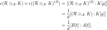 $$\begin{eqnarray}\displaystyle e({\mathcal{R}}\otimes _{A^{\prime }}K)=e(({\mathcal{R}}\otimes _{A^{\prime }}K)^{(d)}) & = & \displaystyle [\vphantom{E_{E_{E}}^{E_{E}}}({\mathcal{R}}\otimes _{A^{\prime }}K)^{(d)}:K[g]\vphantom{E_{E_{E}}^{E_{E}}}]\nonumber\\ \displaystyle & = & \displaystyle \frac{1}{d}[({\mathcal{R}}\otimes _{A^{\prime }}K):K[g]\vphantom{E_{E_{E}}^{E_{E}}}]\nonumber\\ \displaystyle & = & \displaystyle \frac{1}{d}[R[t]:A[t]\vphantom{E_{E_{E}}^{E_{E}}}].\nonumber\end{eqnarray}$$
The last equality holds because
 $$\begin{eqnarray}\text{Quot}(K[g])=\text{Quot}(k[I_{d}t,g])=\text{Quot}(k[I_{d},t])=\text{Quot}(A[t])\end{eqnarray}$$
and
 $\text{Quot}({\mathcal{R}}\otimes _{A^{\prime }}K)=\text{Quot}(R[t])$
. Now we conclude that
$\text{Quot}({\mathcal{R}}\otimes _{A^{\prime }}K)=\text{Quot}(R[t])$
. Now we conclude that
 $$\begin{eqnarray}e({\mathcal{R}}_{~\mathfrak{m}{\mathcal{R}}})=e({\mathcal{R}}\otimes _{A^{\prime }}K)=\frac{1}{d}[R:A]=[B:A].\end{eqnarray}$$
This concludes the proof of the first equality.
The second equality follows from [Reference Simis, Ulrich and Vasconcelos49, 6.1(a) and 3.4]. Here we give a self-contained proof. We write
 ${\mathcal{G}}:=\text{gr}_{I}(R)={\mathcal{R}}/I{\mathcal{R}}$
for the associated graded ring of
${\mathcal{G}}:=\text{gr}_{I}(R)={\mathcal{R}}/I{\mathcal{R}}$
for the associated graded ring of
 $I$
. Notice that
$I$
. Notice that
 ${\mathcal{G}}/\mathfrak{m}{\mathcal{G}}\cong {\mathcal{R}}/\mathfrak{m}{\mathcal{R}}\cong A$
. In particular,
${\mathcal{G}}/\mathfrak{m}{\mathcal{G}}\cong {\mathcal{R}}/\mathfrak{m}{\mathcal{R}}\cong A$
. In particular,
 $\mathfrak{m}{\mathcal{G}}$
is a prime ideal in
$\mathfrak{m}{\mathcal{G}}$
is a prime ideal in
 ${\mathcal{G}}$
and
${\mathcal{G}}$
and
 ${\mathcal{G}}_{\mathfrak{m}{\mathcal{G}}}$
is Artinian, because
${\mathcal{G}}_{\mathfrak{m}{\mathcal{G}}}$
is Artinian, because
 $A$
is a domain and
$A$
is a domain and
 $\text{dim}\,A=s=\text{dim}\,{\mathcal{G}}$
.
$\text{dim}\,A=s=\text{dim}\,{\mathcal{G}}$
.
The
 $j$
-multiplicity of
$j$
-multiplicity of
 $I$
is
$I$
is
 $$\begin{eqnarray}j(I)=e(0:_{{\mathcal{G}}}\mathfrak{m}^{\infty }).\end{eqnarray}$$
Since
 $\text{Supp}_{{\mathcal{G}}}(0:_{{\mathcal{G}}}\mathfrak{m}^{\infty })=V(\mathfrak{m}{\mathcal{G}})$
, the associativity formula for multiplicity 2.7 gives
$\text{Supp}_{{\mathcal{G}}}(0:_{{\mathcal{G}}}\mathfrak{m}^{\infty })=V(\mathfrak{m}{\mathcal{G}})$
, the associativity formula for multiplicity 2.7 gives
 $$\begin{eqnarray}e(0:_{{\mathcal{G}}}\mathfrak{m}^{\infty })=\unicode[STIX]{x1D706}_{{\mathcal{G}}_{\mathfrak{ m}{\mathcal{G}}}}((0:_{{\mathcal{G}}}\mathfrak{m}^{\infty })_{\mathfrak{ m}{\mathcal{G}}})\cdot e({\mathcal{G}}/\mathfrak{m}{\mathcal{G}})=\unicode[STIX]{x1D706}({\mathcal{G}}_{\mathfrak{m}{\mathcal{G}}})\cdot e(A).\end{eqnarray}$$
We conclude that
 $$\begin{eqnarray}j(I)=\unicode[STIX]{x1D706}({\mathcal{G}}_{\mathfrak{m}{\mathcal{G}}})\cdot e(A).\end{eqnarray}$$
(The same equality was proved in [Reference Jeffries, Montaño and Varbaro32, the proof of 3.1].)
If
 $g\not =0$
is an element of
$g\not =0$
is an element of
 $I_{d}$
as above, then
$I_{d}$
as above, then
 $gt\in {\mathcal{R}}\smallsetminus \mathfrak{m}{\mathcal{R}}$
, hence
$gt\in {\mathcal{R}}\smallsetminus \mathfrak{m}{\mathcal{R}}$
, hence
 $I/g=It/gt\subset {\mathcal{R}}$
. It follows that
$I/g=It/gt\subset {\mathcal{R}}$
. It follows that
 $I{\mathcal{R}}_{~\mathfrak{m}{\mathcal{R}}}=g{\mathcal{R}}_{~\mathfrak{m}{\mathcal{R}}}$
, which gives
$I{\mathcal{R}}_{~\mathfrak{m}{\mathcal{R}}}=g{\mathcal{R}}_{~\mathfrak{m}{\mathcal{R}}}$
, which gives
 $$\begin{eqnarray}{\mathcal{G}}_{\mathfrak{m}{\mathcal{G}}}\cong {\mathcal{R}}_{~\mathfrak{m}{\mathcal{G}}}/(g).\end{eqnarray}$$
Now
 $$\begin{eqnarray}\displaystyle \unicode[STIX]{x1D706}(G_{\mathfrak{m}{\mathcal{G}}}) & = & \displaystyle \unicode[STIX]{x1D706}({\mathcal{R}}_{\mathfrak{m}{\mathcal{G}}}/(g))=e(({\mathcal{R}}\otimes _{A^{\prime }}K)/(g))=d\cdot e({\mathcal{R}}\otimes _{A^{\prime }}K)\nonumber\\ \displaystyle & = & \displaystyle d\cdot e({\mathcal{R}}_{\mathfrak{m}{\mathcal{R}}})=d\cdot [B:A].\nonumber\end{eqnarray}$$
We conclude that
 $j(I)=d\cdot [B:A]\cdot e(A)$
.◻
$j(I)=d\cdot [B:A]\cdot e(A)$
.◻
In the next corollary we express the degree of certain dual varieties in terms of the
 $j$
-multiplicity of Jacobian ideals.
$j$
-multiplicity of Jacobian ideals.
Corollary 5.4. Let
 $k$
be an algebraically closed field of characteristic zero, let
$k$
be an algebraically closed field of characteristic zero, let
 $X=V(f)\subset \mathbb{P}_{k}^{n-1}$
be a reduced and irreducible hypersurface of degree
$X=V(f)\subset \mathbb{P}_{k}^{n-1}$
be a reduced and irreducible hypersurface of degree
 $d>1$
, and assume that the dual variety
$d>1$
, and assume that the dual variety
 $X^{\prime }\subset \mathbb{P}_{k}^{n-1^{\prime }}$
is nondeficient, that is, is a hypersurface as well. Let
$X^{\prime }\subset \mathbb{P}_{k}^{n-1^{\prime }}$
is nondeficient, that is, is a hypersurface as well. Let
 $R$
denote the homogeneous coordinate ring of
$R$
denote the homogeneous coordinate ring of
 $X\subset \mathbb{P}_{k}^{n-1}$
, and
$X\subset \mathbb{P}_{k}^{n-1}$
, and
 $I=(\unicode[STIX]{x2202}f/\unicode[STIX]{x2202}x_{1},\ldots ,\unicode[STIX]{x2202}f/\unicode[STIX]{x2202}x_{n})R$
its Jacobian dual. Then
$I=(\unicode[STIX]{x2202}f/\unicode[STIX]{x2202}x_{1},\ldots ,\unicode[STIX]{x2202}f/\unicode[STIX]{x2202}x_{n})R$
its Jacobian dual. Then
 $$\begin{eqnarray}\text{deg}\,X^{\prime }=j(I)/(d-1).\end{eqnarray}$$
Proof. We apply the notation of Data 5.1 to the present setting. The ideal
 $I$
is generated by forms of degree
$I$
is generated by forms of degree
 $d-1$
, and the algebra
$d-1$
, and the algebra
 $A$
is the homogeneous coordinate ring of
$A$
is the homogeneous coordinate ring of
 $X^{\prime }\subset \mathbb{P}_{k}^{n-1^{\prime }}$
. According to [Reference Kleiman, Carrell, Geramita and Russell33, Theorem 4] or [Reference Piene43, Proposition 3.3], the extension
$X^{\prime }\subset \mathbb{P}_{k}^{n-1^{\prime }}$
. According to [Reference Kleiman, Carrell, Geramita and Russell33, Theorem 4] or [Reference Piene43, Proposition 3.3], the extension
 $A\subset B$
is birational, that is,
$A\subset B$
is birational, that is,
 $[B:A]=1$
. Now Theorem 5.3 shows that
$[B:A]=1$
. Now Theorem 5.3 shows that
 $j(I)=(d-1)\text{deg}\,X^{\prime }$
.◻
$j(I)=(d-1)\text{deg}\,X^{\prime }$
.◻
Corollary 5.5. Adopt the data of 5.1. Let
 $J$
be a reduction of
$J$
be a reduction of
 $I$
generated by
$I$
generated by
 $s$
forms of degree
$s$
forms of degree
 $d$
. If the Krull dimension of
$d$
. If the Krull dimension of
 $A$
is equal to
$A$
is equal to
 $s$
, then
$s$
, then
 $$\begin{eqnarray}e(A)=\frac{e({\mathcal{R}}(J)_{\mathfrak{m}{\mathcal{R}}(J)})}{e({\mathcal{R}}(I)_{\mathfrak{m}{\mathcal{R}}(I)})}.\end{eqnarray}$$
Remark.
If
 $k$
is infinite, then
$k$
is infinite, then
 $I$
has a reduction generated by
$I$
has a reduction generated by
 $s$
forms of degree
$s$
forms of degree
 $d$
.
$d$
.
Proof. Notice that
 $k[J_{d}]$
is a homogeneous Noether normalization of
$k[J_{d}]$
is a homogeneous Noether normalization of
 $A=k[I_{d}]$
. Therefore,
$A=k[I_{d}]$
. Therefore,
 $e(A)=[k[I_{d}]:k[J_{d}]]$
. On the other hand,
$e(A)=[k[I_{d}]:k[J_{d}]]$
. On the other hand,
 $$\begin{eqnarray}[k[I_{d}]:k[J_{d}]]=\frac{[B:k[J_{d}]]}{[B:k[I_{d}]]}=\frac{e({\mathcal{R}}(J)_{\mathfrak{m}{\mathcal{R}}(J)})}{e({\mathcal{R}}(I)_{\mathfrak{m}{\mathcal{R}}(I)})},\end{eqnarray}$$
where the last equality follows from Theorem 5.3 applied to the two ideals
 $J$
and
$J$
and
 $I$
, respectively.◻
$I$
, respectively.◻
As a consequence we obtain the following numerical criterion for birationality in terms of the Rees ring or the special fiber ring, respectively.
Corollary 5.6. Adopt the data of 5.1. The following statements are equivalent.
-
(1) The ring extension
$A\subset B$
is birational, that is,
$[B:A]=1$
. -
(2) The ring
${\mathcal{R}}(I)_{\mathfrak{m}{\mathcal{R}}(I)}$
is a discrete valuation ring. -
(3) The ring
$A$
has dimension
$s$
and
$e(A)=e({\mathcal{R}}(J)_{\mathfrak{m}{\mathcal{R}}(J)})$
, where
$J$
is a reduction of
$I$
generated by
$s$
forms of degree
$d$
.


Proof. Notice that if the ring extension
 $A\subset B$
is birational, then
$A\subset B$
is birational, then
 $A$
and
$A$
and
 $B$
have the same transcendence degree over
$B$
have the same transcendence degree over
 $k$
and therefore,
$k$
and therefore,
 $\text{dim}\,A=\text{dim}\,B=s$
. Furthermore,
$\text{dim}\,A=\text{dim}\,B=s$
. Furthermore,
 $\text{dim}\,{\mathcal{R}}(I)_{\mathfrak{m}{\mathcal{R}}(I)}=1$
if and only if
$\text{dim}\,{\mathcal{R}}(I)_{\mathfrak{m}{\mathcal{R}}(I)}=1$
if and only if
 $\text{dim}\,A=s$
according to Remark 5.2. Now the asserted equivalences follow from Theorem 5.3 and Corollary 5.5.◻
$\text{dim}\,A=s$
according to Remark 5.2. Now the asserted equivalences follow from Theorem 5.3 and Corollary 5.5.◻
More can be said if the rational map
 $\unicode[STIX]{x1D6F9}$
of data of 3.1 is a morphism, or equivalently, if the ideal
$\unicode[STIX]{x1D6F9}$
of data of 3.1 is a morphism, or equivalently, if the ideal
 $I$
is
$I$
is
 $\mathfrak{m}$
-primary. A crucial statement in the following corollary is the statement about canonical modules. Indeed, cores, adjoints, and
$\mathfrak{m}$
-primary. A crucial statement in the following corollary is the statement about canonical modules. Indeed, cores, adjoints, and
 $S_{2}$
-fications are all constructed using the canonical module of the Rees ring.
$S_{2}$
-fications are all constructed using the canonical module of the Rees ring.
Remark 5.7. If
 $I$
is an
$I$
is an
 $\mathfrak{m}$
-primary ideal generated by forms of degree
$\mathfrak{m}$
-primary ideal generated by forms of degree
 $d$
, then the ideal
$d$
, then the ideal
 $\mathfrak{m}^{d}$
is integral over
$\mathfrak{m}^{d}$
is integral over
 $I$
. Hence the ring extension
$I$
. Hence the ring extension
 $$\begin{eqnarray}{\mathcal{R}}(I)\subset {\mathcal{R}}(\mathfrak{m}^{d})\end{eqnarray}$$
is not only birational, but also module-finite. Thus applying the functor
 $-^{\vee }=\text{Hom}_{{\mathcal{R}}(I)}(-,\unicode[STIX]{x1D714}_{{\mathcal{R}}(I)})$
induces a containment of the canonical modules
$-^{\vee }=\text{Hom}_{{\mathcal{R}}(I)}(-,\unicode[STIX]{x1D714}_{{\mathcal{R}}(I)})$
induces a containment of the canonical modules
 $$\begin{eqnarray}\unicode[STIX]{x1D714}_{{\mathcal{R}}(\mathfrak{m}^{d})}\subset \unicode[STIX]{x1D714}_{{\mathcal{R}}(I)},\end{eqnarray}$$
and evaluating
 $-^{\vee }$
twice yields an inclusion of the
$-^{\vee }$
twice yields an inclusion of the
 $S_{2}$
-ifications
$S_{2}$
-ifications
 $$\begin{eqnarray}\operatorname{End}_{{\mathcal{R}}(I)}(\unicode[STIX]{x1D714}_{{\mathcal{R}}(I)})\subset \operatorname{End}_{{\mathcal{R}}(\mathfrak{m}^{d})}(\unicode[STIX]{x1D714}_{{\mathcal{R}}(\mathfrak{m}^{d})}).\end{eqnarray}$$
Applying
 $-^{\vee }$
once more to last inclusion returns the previous one. In particular, one of the two last inclusions is an equality if and only if the other is.
$-^{\vee }$
once more to last inclusion returns the previous one. In particular, one of the two last inclusions is an equality if and only if the other is.
Corollary 5.8. Adopt the data of 3.1. In addition, assume that
 $I$
is
$I$
is
 $\mathfrak{m}$
-primary and the field
$\mathfrak{m}$
-primary and the field
 $k$
is infinite. Statements (1)–(5) are equivalent.
$k$
is infinite. Statements (1)–(5) are equivalent.
-
(1) The morphism
$\unicode[STIX]{x1D6F9}$
is birational onto its image, that is,
$[B:A]=1$
. -
(2) The Rees ring
${\mathcal{R}}(I)$
satisfies Serre’s condition
$(R_{1})$
. -
(3)
$\unicode[STIX]{x1D714}_{{\mathcal{R}}(I)}=\unicode[STIX]{x1D714}_{{\mathcal{R}}(\mathfrak{m}^{d})}$
. -
(4)
$\operatorname{End}_{{\mathcal{R}}(I)}(\unicode[STIX]{x1D714}_{{\mathcal{R}}(I)})=\operatorname{End}_{{\mathcal{R}}(\mathfrak{m}^{d})}(\unicode[STIX]{x1D714}_{{\mathcal{R}}(\mathfrak{m}^{d})})$
. -
(5)
$e(A)=d^{s-1}$
.Furthermore, statements (1)–(5) all imply
-
(6)
$\text{gradedcore}(I)=\text{core}(I)=\text{core}(\mathfrak{m}^{d})=\mathfrak{m}^{(d-1)s+1}=\text{adj}(I^{s})$
. -
(7) If
${\mathcal{R}}(I)$
satisfies Serre’s property
$(S_{2})$
, then
${\mathcal{R}}(I)$
is Cohen–Macaulay.


Proof. Since
 $I$
is
$I$
is
 $\mathfrak{m}$
-primary the ring
$\mathfrak{m}$
-primary the ring
 $A$
has Krull dimension
$A$
has Krull dimension
 $s$
. In particular,
$s$
. In particular,
 $\mathfrak{m}{\mathcal{R}}(I)$
is a prime ideal of height one. If
$\mathfrak{m}{\mathcal{R}}(I)$
is a prime ideal of height one. If
 $Q$
is any other height one prime ideal of
$Q$
is any other height one prime ideal of
 ${\mathcal{R}}(I)$
, then
${\mathcal{R}}(I)$
, then
 $Q$
does not contain
$Q$
does not contain
 $\mathfrak{m}$
and hence does not contain
$\mathfrak{m}$
and hence does not contain
 $I$
. It follows that
$I$
. It follows that
 ${\mathcal{R}}(I)_{Q}$
is regular. Thus
${\mathcal{R}}(I)_{Q}$
is regular. Thus
 ${\mathcal{R}}(I)$
satisfies Serre’s condition
${\mathcal{R}}(I)$
satisfies Serre’s condition
 $(R_{1})$
if and only if
$(R_{1})$
if and only if
 ${\mathcal{R}}(I)_{\mathfrak{m}{\mathcal{R}}(I)}$
is a discrete valuation ring. Now the equivalence of (1) and (2) follows from Corollary 5.6.
${\mathcal{R}}(I)_{\mathfrak{m}{\mathcal{R}}(I)}$
is a discrete valuation ring. Now the equivalence of (1) and (2) follows from Corollary 5.6.
To see the equivalence of (2) and (3) notice that
 ${\mathcal{R}}(\mathfrak{m}^{d})$
is the integral closure of
${\mathcal{R}}(\mathfrak{m}^{d})$
is the integral closure of
 ${\mathcal{R}}(I)$
. Hence
${\mathcal{R}}(I)$
. Hence
 ${\mathcal{R}}(I)$
satisfies Serre’s condition
${\mathcal{R}}(I)$
satisfies Serre’s condition
 $(R_{1})$
if and only if the
$(R_{1})$
if and only if the
 ${\mathcal{R}}(I)$
-module
${\mathcal{R}}(I)$
-module
 ${\mathcal{R}}(\mathfrak{m}^{d})/{\mathcal{R}}(I)$
has codimension at least two, which in turn is equivalent to the equality
${\mathcal{R}}(\mathfrak{m}^{d})/{\mathcal{R}}(I)$
has codimension at least two, which in turn is equivalent to the equality
 $\unicode[STIX]{x1D714}_{{\mathcal{R}}(I)}=\unicode[STIX]{x1D714}_{{\mathcal{R}}(\mathfrak{m}^{d})}$
. The second equivalence is obtained by analyzing the long exact sequence of
$\unicode[STIX]{x1D714}_{{\mathcal{R}}(I)}=\unicode[STIX]{x1D714}_{{\mathcal{R}}(\mathfrak{m}^{d})}$
. The second equivalence is obtained by analyzing the long exact sequence of
 $\text{Ext}_{R\otimes _{k}S}^{\bullet }(-,\unicode[STIX]{x1D714}_{R\otimes _{k}S})$
associated to the short exact sequence
$\text{Ext}_{R\otimes _{k}S}^{\bullet }(-,\unicode[STIX]{x1D714}_{R\otimes _{k}S})$
associated to the short exact sequence
 $$\begin{eqnarray}0\longrightarrow {\mathcal{R}}(I)\longrightarrow {\mathcal{R}}(\mathfrak{m}^{d})\longrightarrow {\mathcal{R}}(\mathfrak{m}^{d})/{\mathcal{R}}(I)\longrightarrow 0\end{eqnarray}$$
and bearing in mind that
 ${\mathcal{R}}(\mathfrak{m}^{d})$
is Cohen–Macaulay. The equivalence of (3) and (4) is explained in Remark 5.7.
${\mathcal{R}}(\mathfrak{m}^{d})$
is Cohen–Macaulay. The equivalence of (3) and (4) is explained in Remark 5.7.
To see that (5) is equivalent to the other statements we apply Corollary 5.6. We may assume that
 $k$
is infinite. It suffices to show the equality
$k$
is infinite. It suffices to show the equality
 $e({\mathcal{R}}(J)_{\mathfrak{m}{\mathcal{R}}(J)})=d^{s-1}$
for the ideal
$e({\mathcal{R}}(J)_{\mathfrak{m}{\mathcal{R}}(J)})=d^{s-1}$
for the ideal
 $J$
of Corollary 5.6. Since
$J$
of Corollary 5.6. Since
 $I$
is
$I$
is
 $\mathfrak{m}$
-primary, the ideal
$\mathfrak{m}$
-primary, the ideal
 $J$
is generated by a regular sequence of
$J$
is generated by a regular sequence of
 $s$
forms of degree
$s$
forms of degree
 $d$
. Therefore,
$d$
. Therefore,
 $[R:k[J_{d}]]=d^{s}$
and then
$[R:k[J_{d}]]=d^{s}$
and then
 $e({\mathcal{R}}(J)_{\mathfrak{m}{\mathcal{R}}(J)})=[B:k[J_{d}]]=d^{s-1}$
according to Theorem 5.3.
$e({\mathcal{R}}(J)_{\mathfrak{m}{\mathcal{R}}(J)})=[B:k[J_{d}]]=d^{s-1}$
according to Theorem 5.3.
We now show that (2) implies (6). We will repeatedly use the fact from [Reference Polini, Ulrich and Vitulli45, 2.1] that the core of
 $\mathfrak{m}$
-primary ideals localizes. The first equality follows from [Reference Corso, Polini and Ulrich12, 4.5] as
$\mathfrak{m}$
-primary ideals localizes. The first equality follows from [Reference Corso, Polini and Ulrich12, 4.5] as
 $I$
is generated by forms of the same degree. Recall that the Rees ring
$I$
is generated by forms of the same degree. Recall that the Rees ring
 $R[It]$
and the extended Rees ring
$R[It]$
and the extended Rees ring
 $R[It,t^{-1}]$
have isomorphic projective spectra. Hence if the Rees ring satisfies
$R[It,t^{-1}]$
have isomorphic projective spectra. Hence if the Rees ring satisfies
 $R_{1}$
, then so does
$R_{1}$
, then so does
 $\operatorname{Proj}(R[It,t^{-1}])$
. It follows that
$\operatorname{Proj}(R[It,t^{-1}])$
. It follows that
 $R[It,t^{-1}]$
satisfies
$R[It,t^{-1}]$
satisfies
 $R_{1}$
as well because it suffices to consider prime ideals containing
$R_{1}$
as well because it suffices to consider prime ideals containing
 $t^{-1}$
and because the ideal
$t^{-1}$
and because the ideal
 $(It,t^{-1})R[It,t^{-1}]$
has height
$(It,t^{-1})R[It,t^{-1}]$
has height
 $s+1>1$
. One uses the argument that (2) implies (3) to see that the
$s+1>1$
. One uses the argument that (2) implies (3) to see that the
 $R_{1}$
property of the extended Rees ring implies the bigraded isomorphism
$R_{1}$
property of the extended Rees ring implies the bigraded isomorphism
 $$\begin{eqnarray}\unicode[STIX]{x1D714}_{R[It,t^{-1}]}\cong \unicode[STIX]{x1D714}_{R[\mathfrak{m}^{d}t,t^{-1}]}.\end{eqnarray}$$
By [Reference Polini and Ulrich44, 2.2] and [Reference Fouli, Polini and Ulrich20, 1.2] the core can be recovered from the canonical module of the extended Rees ring. Therefore,
 $\operatorname{core}(I)=\operatorname{core}(\mathfrak{m}^{d})$
, which is the second equality in (6). The third equality follows from [Reference Corso, Polini and Ulrich13, 4.2]. Finally, one has
$\operatorname{core}(I)=\operatorname{core}(\mathfrak{m}^{d})$
, which is the second equality in (6). The third equality follows from [Reference Corso, Polini and Ulrich13, 4.2]. Finally, one has
 $\mathfrak{m}^{(d-1)s+1}=\text{adj}(\mathfrak{m}^{ds})$
by [Reference Lipman40, 1.3.2(c)] and
$\mathfrak{m}^{(d-1)s+1}=\text{adj}(\mathfrak{m}^{ds})$
by [Reference Lipman40, 1.3.2(c)] and
 $\text{adj}(\mathfrak{m}^{ds})=\text{adj}\,(I^{s})$
because
$\text{adj}(\mathfrak{m}^{ds})=\text{adj}\,(I^{s})$
because
 $\mathfrak{m}^{ds}$
is integral over
$\mathfrak{m}^{ds}$
is integral over
 $I^{s}$
.
$I^{s}$
.
To see (7), notice that
 ${\mathcal{R}}(I)$
is normal, hence
${\mathcal{R}}(I)$
is normal, hence
 ${\mathcal{R}}(I)={\mathcal{R}}(\mathfrak{m}^{d})$
. The last ring is Cohen–Macaulay because it is a direct summand of
${\mathcal{R}}(I)={\mathcal{R}}(\mathfrak{m}^{d})$
. The last ring is Cohen–Macaulay because it is a direct summand of
 ${\mathcal{R}}(\mathfrak{m})$
, which is a Cohen–Macaulay ring and a finitely generated module over
${\mathcal{R}}(\mathfrak{m})$
, which is a Cohen–Macaulay ring and a finitely generated module over
 ${\mathcal{R}}(\mathfrak{m}^{d})$
.◻
${\mathcal{R}}(\mathfrak{m}^{d})$
.◻
The canonical module and the
 $S_{2}$
-ification of
$S_{2}$
-ification of
 ${\mathcal{R}}(m^{d})$
that appear in Corollary 5.8 are known explicitly.
${\mathcal{R}}(m^{d})$
that appear in Corollary 5.8 are known explicitly.
Remark 5.9. Let
 $R=k[x_{1},\ldots ,x_{s}]$
be a standard-graded polynomial ring in
$R=k[x_{1},\ldots ,x_{s}]$
be a standard-graded polynomial ring in
 $s$
variables over a field
$s$
variables over a field
 $k$
, with maximal homogeneous ideal
$k$
, with maximal homogeneous ideal
 $\mathfrak{m}$
. Let
$\mathfrak{m}$
. Let
 $d$
be a positive integer and write
$d$
be a positive integer and write
 $s-1=qd+r$
where
$s-1=qd+r$
where
 $q$
and
$q$
and
 $r$
are nonnegative integers with
$r$
are nonnegative integers with
 $r<d$
. The bigraded canonical module of the Rees ring of
$r<d$
. The bigraded canonical module of the Rees ring of
 $\mathfrak{m}^{d}$
is
$\mathfrak{m}^{d}$
is
 $$\begin{eqnarray}\unicode[STIX]{x1D714}_{{\mathcal{R}}(\mathfrak{m}^{d})}=\left\{\begin{array}{@{}ll@{}}x_{1}^{s}t\mathfrak{m}^{d-s+1}{\mathcal{R}}(\mathfrak{m}^{d})\quad & \text{if }s\leqslant d,\\ x_{1}^{s}t((1,t)^{q-1},\mathfrak{m}^{d-r}t^{q}){\mathcal{R}}(\mathfrak{m}^{d})\quad & \text{if }d<s.\end{array}\right.\end{eqnarray}$$
Furthermore, the natural inclusion
 ${\mathcal{R}}(m^{d})\subset \operatorname{End}_{{\mathcal{R}}(m^{d})}(\unicode[STIX]{x1D714}_{{\mathcal{R}}(m^{d})})$
is an equality.
${\mathcal{R}}(m^{d})\subset \operatorname{End}_{{\mathcal{R}}(m^{d})}(\unicode[STIX]{x1D714}_{{\mathcal{R}}(m^{d})})$
is an equality.
Proof. From the presentation of the Rees ring
 $$\begin{eqnarray}{\mathcal{R}}(\mathfrak{m})=\frac{R[T_{1},\ldots ,T_{s}]}{I_{2}\left(\left[\begin{array}{@{}ccc@{}}x_{1} & \ldots & x_{s}\\ T_{1} & \ldots & T_{s}\end{array}\right]\right)}\end{eqnarray}$$
one computes
 $$\begin{eqnarray}\unicode[STIX]{x1D714}_{{\mathcal{R}}(\mathfrak{m})}\cong x_{1}^{2}t(x_{1},x_{1}t)^{s-2}{\mathcal{R}}(\mathfrak{m}),\end{eqnarray}$$
where the factor
 $x_{1}^{2}t$
is required to make the isomorphism bihomogeneous. The Rees ring
$x_{1}^{2}t$
is required to make the isomorphism bihomogeneous. The Rees ring
 ${\mathcal{R}}(\mathfrak{m}^{d})$
is obtained by taking the
${\mathcal{R}}(\mathfrak{m}^{d})$
is obtained by taking the
 $d$
-Veronese subring of
$d$
-Veronese subring of
 ${\mathcal{R}}(\mathfrak{m})$
with respect to the grading given by the
${\mathcal{R}}(\mathfrak{m})$
with respect to the grading given by the
 $T$
-variables and then rescaling the grading. Since the Veronese functor commutes with taking canonical modules, we obtain the desired statement.
$T$
-variables and then rescaling the grading. Since the Veronese functor commutes with taking canonical modules, we obtain the desired statement.
The natural inclusion
 ${\mathcal{R}}(m^{d})\subset \operatorname{End}_{{\mathcal{R}}(m^{d})}(\unicode[STIX]{x1D714}_{{\mathcal{R}}(m^{d})})$
is an equality because
${\mathcal{R}}(m^{d})\subset \operatorname{End}_{{\mathcal{R}}(m^{d})}(\unicode[STIX]{x1D714}_{{\mathcal{R}}(m^{d})})$
is an equality because
 ${\mathcal{R}}(m^{d})$
is Cohen–Macaulay and
${\mathcal{R}}(m^{d})$
is Cohen–Macaulay and
 $\operatorname{End}_{{\mathcal{R}}(m^{d})}(\unicode[STIX]{x1D714}_{{\mathcal{R}}(m^{d})})$
is its
$\operatorname{End}_{{\mathcal{R}}(m^{d})}(\unicode[STIX]{x1D714}_{{\mathcal{R}}(m^{d})})$
is its
 $S_{2}$
-ification.◻
$S_{2}$
-ification.◻
In Corollaries 5.11 and 5.12 we extend the equivalence
 $(1)\;\Longleftrightarrow \;(2)$
from Corollary 5.8. We begin by comparing the heights of conductors for certain extensions of Rees rings and special fiber rings.
$(1)\;\Longleftrightarrow \;(2)$
from Corollary 5.8. We begin by comparing the heights of conductors for certain extensions of Rees rings and special fiber rings.
Proposition 5.10. Adopt the data of 5.1. In addition, assume that
 $I$
is
$I$
is
 $\mathfrak{m}$
-primary. Let
$\mathfrak{m}$
-primary. Let
 $K$
be an ideal of
$K$
be an ideal of
 $R$
which is generated by forms of degree
$R$
which is generated by forms of degree
 $d$
and which contains
$d$
and which contains
 $I$
. Write
$I$
. Write
 $C$
for
$C$
for
 $k[K_{d}]$
; so,
$k[K_{d}]$
; so,
 $A=k[I_{d}]\subset C=k[K_{d}]$
. Then
$A=k[I_{d}]\subset C=k[K_{d}]$
. Then
 $$\begin{eqnarray}\operatorname{ht}({\mathcal{R}}(I):_{{\mathcal{R}}(I)}{\mathcal{R}}(K))=1+\operatorname{ht}(A:_{A}C)=1+\operatorname{ht}({\mathcal{F}}(I):_{{\mathcal{F}}(I)}{\mathcal{F}}(K)).\end{eqnarray}$$
Proof. Let
 $A^{\prime }$
be the subring
$A^{\prime }$
be the subring
 $k[I_{d}t]$
of
$k[I_{d}t]$
of
 ${\mathcal{R}}(I)=R[I_{d}t]$
and
${\mathcal{R}}(I)=R[I_{d}t]$
and
 $C^{\prime }$
be the subring
$C^{\prime }$
be the subring
 $k[K_{d}t]$
of
$k[K_{d}t]$
of
 ${\mathcal{R}}(K)=R[K_{d}t]$
. We first prove that the ideals
${\mathcal{R}}(K)=R[K_{d}t]$
. We first prove that the ideals
 $$\begin{eqnarray}\operatorname{rad}({\mathcal{R}}(I):_{{\mathcal{R}}(I)}{\mathcal{R}}(K))\quad \text{and}\quad \operatorname{rad}((\mathfrak{m},A^{\prime }:_{A^{\prime }}C^{\prime }){\mathcal{R}}(I))\end{eqnarray}$$
of
 ${\mathcal{R}}(I)$
are equal.
${\mathcal{R}}(I)$
are equal.
We prove the inclusion “
 $\supset$
” for the ideals of (5.10.1). The Rees algebra
$\supset$
” for the ideals of (5.10.1). The Rees algebra
 ${\mathcal{R}}(K)$
is a module-finite extension of
${\mathcal{R}}(K)$
is a module-finite extension of
 ${\mathcal{R}}(I)$
because
${\mathcal{R}}(I)$
because
 $I$
is
$I$
is
 $\mathfrak{m}$
-primary; hence,
$\mathfrak{m}$
-primary; hence,
 $I$
is a reduction of
$I$
is a reduction of
 $K$
and there is a positive integer
$K$
and there is a positive integer
 $t$
with
$t$
with
 $K^{t}K^{n}\subset I^{n}$
for all nonnegative integers
$K^{t}K^{n}\subset I^{n}$
for all nonnegative integers
 $n$
. It follows that
$n$
. It follows that
 $K^{t}\subset {\mathcal{R}}(I):_{{\mathcal{R}}(I)}{\mathcal{R}}(K)$
; and therefore,
$K^{t}\subset {\mathcal{R}}(I):_{{\mathcal{R}}(I)}{\mathcal{R}}(K)$
; and therefore,
 $\mathfrak{m}\subset \operatorname{rad}({\mathcal{R}}(I):_{{\mathcal{R}}(I)}{\mathcal{R}}(K))$
. Clearly,
$\mathfrak{m}\subset \operatorname{rad}({\mathcal{R}}(I):_{{\mathcal{R}}(I)}{\mathcal{R}}(K))$
. Clearly,
 $A^{\prime }:_{A^{\prime }}C^{\prime }\subset {\mathcal{R}}(I):_{{\mathcal{R}}(I)}{\mathcal{R}}(K)$
because
$A^{\prime }:_{A^{\prime }}C^{\prime }\subset {\mathcal{R}}(I):_{{\mathcal{R}}(I)}{\mathcal{R}}(K)$
because
 ${\mathcal{R}}(I)=R[A^{\prime }]$
and
${\mathcal{R}}(I)=R[A^{\prime }]$
and
 ${\mathcal{R}}(K)=R[C^{\prime }]$
.
${\mathcal{R}}(K)=R[C^{\prime }]$
.
We prove the inclusion “
 $\subset$
” for the ideals of (5.10.1). Let
$\subset$
” for the ideals of (5.10.1). Let
 $\unicode[STIX]{x1D6FC}$
be a bihomogeneous element of
$\unicode[STIX]{x1D6FC}$
be a bihomogeneous element of
 ${\mathcal{R}}(I):_{{\mathcal{R}}(I)}{\mathcal{R}}(K)$
. In particular,
${\mathcal{R}}(I):_{{\mathcal{R}}(I)}{\mathcal{R}}(K)$
. In particular,
 $\unicode[STIX]{x1D6FC}=ft^{j}$
for some homogeneous form
$\unicode[STIX]{x1D6FC}=ft^{j}$
for some homogeneous form
 $f$
in
$f$
in
 $I$
and some nonnegative integer
$I$
and some nonnegative integer
 $j$
. If the homogeneous form
$j$
. If the homogeneous form
 $f$
has degree
$f$
has degree
 $i+dj$
as a polynomial in
$i+dj$
as a polynomial in
 $R=k[x_{1},\ldots ,x_{s}]$
, then the bi-degree of
$R=k[x_{1},\ldots ,x_{s}]$
, then the bi-degree of
 $\unicode[STIX]{x1D6FC}$
in
$\unicode[STIX]{x1D6FC}$
in
 ${\mathcal{R}}(I)$
is
${\mathcal{R}}(I)$
is
 $(i,j)$
. If
$(i,j)$
. If
 $i$
is positive, then
$i$
is positive, then
 $\unicode[STIX]{x1D6FC}$
is in
$\unicode[STIX]{x1D6FC}$
is in
 $\mathfrak{m}{\mathcal{R}}(I)$
. If
$\mathfrak{m}{\mathcal{R}}(I)$
. If
 $i=0$
, then
$i=0$
, then
 $\unicode[STIX]{x1D6FC}$
is in
$\unicode[STIX]{x1D6FC}$
is in
 $A^{\prime }$
and
$A^{\prime }$
and
 $\unicode[STIX]{x1D6FC}\cdot C^{\prime }\subset \unicode[STIX]{x1D6FC}\cdot {\mathcal{R}}(K)\subset {\mathcal{R}}(I)$
. One may compute
$\unicode[STIX]{x1D6FC}\cdot C^{\prime }\subset \unicode[STIX]{x1D6FC}\cdot {\mathcal{R}}(K)\subset {\mathcal{R}}(I)$
. One may compute
 $x$
-degree to see that
$x$
-degree to see that
 $\unicode[STIX]{x1D6FC}\cdot C^{\prime }$
is actually contained in
$\unicode[STIX]{x1D6FC}\cdot C^{\prime }$
is actually contained in
 $A^{\prime }$
. In either case,
$A^{\prime }$
. In either case,
 $\unicode[STIX]{x1D6FC}\in (\mathfrak{m},A^{\prime }:_{A^{\prime }}C^{\prime }){\mathcal{R}}(I)$
.
$\unicode[STIX]{x1D6FC}\in (\mathfrak{m},A^{\prime }:_{A^{\prime }}C^{\prime }){\mathcal{R}}(I)$
.
Now that the assertion of (5.10.1) has been established, we complete the proof of the result by applying the natural quotient homomorphism
 ${\mathcal{R}}(I)\rightarrow {\mathcal{R}}(I)/\mathfrak{m}{\mathcal{R}}(I)$
to the ideals of (5.10.1). The ring
${\mathcal{R}}(I)\rightarrow {\mathcal{R}}(I)/\mathfrak{m}{\mathcal{R}}(I)$
to the ideals of (5.10.1). The ring
 ${\mathcal{R}}(I)$
is a domain and a finitely generated algebra over a field, and the ideal
${\mathcal{R}}(I)$
is a domain and a finitely generated algebra over a field, and the ideal
 $\mathfrak{m}{\mathcal{R}}(I)$
of
$\mathfrak{m}{\mathcal{R}}(I)$
of
 ${\mathcal{R}}(I)$
has height
${\mathcal{R}}(I)$
has height
 $1$
. Thus,
$1$
. Thus,
 $$\begin{eqnarray}\begin{array}{@{}lllll@{}}\operatorname{ht}({\mathcal{R}}(I):_{{\mathcal{R}}(I)}{\mathcal{R}}(K))-1\, & =\, & \operatorname{ht}\frac{\operatorname{rad}({\mathcal{R}}(I):_{{\mathcal{R}}(I)}{\mathcal{R}}(K))}{\mathfrak{m}{\mathcal{R}}(I)}\, & =\, & \operatorname{ht}(\mathfrak{m},A^{\prime }:_{A^{\prime }}C^{\prime })\frac{{\mathcal{R}}(I)}{\mathfrak{m}{\mathcal{R}}(I)}\\ \, & =\, & \operatorname{ht}({\mathcal{F}}(I):_{{\mathcal{F}}(I)}{\mathcal{F}}(K))\, & =\, & \operatorname{ht}(A:_{A}C).\end{array}\end{eqnarray}$$
Corollary 5.11. Adopt the data of 5.1. In addition, assume that
 $R=k[x_{1},\ldots ,x_{s}]$
and
$R=k[x_{1},\ldots ,x_{s}]$
and
 $I$
is
$I$
is
 $\mathfrak{m}$
-primary. Let
$\mathfrak{m}$
-primary. Let
 $i\leqslant s$
be a fixed positive integer. Then, the following conditions are equivalent.
$i\leqslant s$
be a fixed positive integer. Then, the following conditions are equivalent.
-
(a)
${\mathcal{R}}(I)$
satisfies the Serre condition
$(R_{i})$
. -
(b)
$A$
satisfies the Serre condition
$(R_{i-1})$
and
$A\subset B$
is a birational extension.


Proof. When
 $i=1$
, the statement is
$i=1$
, the statement is
 $(1)\;\Longleftrightarrow \;(2)$
from Corollary 5.8. Henceforth, we assume
$(1)\;\Longleftrightarrow \;(2)$
from Corollary 5.8. Henceforth, we assume
 $2\leqslant i$
and that
$2\leqslant i$
and that
 $A\subset B$
is a birational extension. Thus, both extensions
$A\subset B$
is a birational extension. Thus, both extensions
 ${\mathcal{R}}(I)\subset {\mathcal{R}}(\mathfrak{m}^{d})$
and
${\mathcal{R}}(I)\subset {\mathcal{R}}(\mathfrak{m}^{d})$
and
 $A\subset B$
are module-finite and birational.
$A\subset B$
are module-finite and birational.
Moreover,
 $\dim {\mathcal{R}}(I)=s+1$
and
$\dim {\mathcal{R}}(I)=s+1$
and
 ${\mathcal{R}}(\mathfrak{m}^{d})$
has an isolated singularity. Hence for any prime ideal
${\mathcal{R}}(\mathfrak{m}^{d})$
has an isolated singularity. Hence for any prime ideal
 $Q$
of
$Q$
of
 ${\mathcal{R}}(I)$
with
${\mathcal{R}}(I)$
with
 $\dim {\mathcal{R}}(I)_{Q}\leqslant s$
, the ring
$\dim {\mathcal{R}}(I)_{Q}\leqslant s$
, the ring
 ${\mathcal{R}}(I)_{Q}$
is regular if and only if
${\mathcal{R}}(I)_{Q}$
is regular if and only if
 ${\mathcal{R}}(I)_{Q}={\mathcal{R}}(\mathfrak{m}^{d})_{Q}$
. This shows that
${\mathcal{R}}(I)_{Q}={\mathcal{R}}(\mathfrak{m}^{d})_{Q}$
. This shows that
 ${\mathcal{R}}(I)$
satisfies
${\mathcal{R}}(I)$
satisfies
 $(R_{i})$
if and only if
$(R_{i})$
if and only if
 $i<\operatorname{ht}({\mathcal{R}}(I):_{{\mathcal{R}}(I)}{\mathcal{R}}(\mathfrak{m}^{d}))$
.
$i<\operatorname{ht}({\mathcal{R}}(I):_{{\mathcal{R}}(I)}{\mathcal{R}}(\mathfrak{m}^{d}))$
.
Similarly,
 $\dim A=s$
and
$\dim A=s$
and
 $B$
has an isolated singularity. Hence again,
$B$
has an isolated singularity. Hence again,
 $A_{q}$
is regular if and only if
$A_{q}$
is regular if and only if
 $A_{q}=B_{q}$
for any prime ideal
$A_{q}=B_{q}$
for any prime ideal
 $q$
of
$q$
of
 $A$
with
$A$
with
 $\dim A_{q}\leqslant s-1$
. We conclude that
$\dim A_{q}\leqslant s-1$
. We conclude that
 $A$
satisfies
$A$
satisfies
 $(R_{i-1})$
if and only if
$(R_{i-1})$
if and only if
 $i-1<\operatorname{ht}(A:_{A}B)$
.
$i-1<\operatorname{ht}(A:_{A}B)$
.
Apply Proposition 5.10, with
 $K=\mathfrak{m}^{d}$
to complete the proof.◻
$K=\mathfrak{m}^{d}$
to complete the proof.◻
In the situation of Data 3.1,
 $A$
is the homogeneous coordinate ring of the image of
$A$
is the homogeneous coordinate ring of the image of
 $\unicode[STIX]{x1D6F9}$
. The following geometric consequence of Corollary 5.11 is now immediate.
$\unicode[STIX]{x1D6F9}$
. The following geometric consequence of Corollary 5.11 is now immediate.
Corollary 5.12. Adopt the data of 3.1. In addition assume that
 $I$
is
$I$
is
 $\mathfrak{m}$
-primary. Then the Rees ring
$\mathfrak{m}$
-primary. Then the Rees ring
 ${\mathcal{R}}(I)$
has an isolated singularity if and only if the image of
${\mathcal{R}}(I)$
has an isolated singularity if and only if the image of
 $\unicode[STIX]{x1D6F9}$
is smooth and
$\unicode[STIX]{x1D6F9}$
is smooth and
 $\unicode[STIX]{x1D6F9}$
is birational onto its image.
$\unicode[STIX]{x1D6F9}$
is birational onto its image.
For
 $s=2$
we harvest consequences about canonical modules,
$s=2$
we harvest consequences about canonical modules,
 $S_{2}$
-fications, and cores for any ideal generated by forms of the same degree. Indeed, when
$S_{2}$
-fications, and cores for any ideal generated by forms of the same degree. Indeed, when
 $s=2$
we can pass by way of a faithfully flat descent to the birational situation according to Corollary 4.5. We compute canonical modules,
$s=2$
we can pass by way of a faithfully flat descent to the birational situation according to Corollary 4.5. We compute canonical modules,
 $S_{2}$
-fications, and cores in the birational situation using Corollary 5.8 and Remark 5.9. We can pull these objects back because they are preserved under faithfully flat extensions, whereas adjoint ideals are not preserved under such extensions.
$S_{2}$
-fications, and cores in the birational situation using Corollary 5.8 and Remark 5.9. We can pull these objects back because they are preserved under faithfully flat extensions, whereas adjoint ideals are not preserved under such extensions.
Theorem 5.13. Adopt the data of 5.1. In addition assume that
 $R=k[x_{1},x_{2}]$
is a polynomial ring in two variables over an infinite field and
$R=k[x_{1},x_{2}]$
is a polynomial ring in two variables over an infinite field and
 $I$
is
$I$
is
 $\mathfrak{m}$
-primary. Write
$\mathfrak{m}$
-primary. Write
 $r=[B:A]$
and let
$r=[B:A]$
and let
 $f_{1}$
and
$f_{1}$
and
 $f_{2}$
be the forms in
$f_{2}$
be the forms in
 $R$
of degree
$R$
of degree
 $r$
of Corollary 4.5. The following statements hold.
$r$
of Corollary 4.5. The following statements hold.
-
(1)
$\unicode[STIX]{x1D714}_{{\mathcal{R}}(I)}=\unicode[STIX]{x1D714}_{{\mathcal{R}}((f_{1},f_{2})^{d/r})}=f_{1}^{2}t(f_{1},f_{2})^{(d/r)-1}{\mathcal{R}}((f_{1},f_{2})^{d/r})$
. -
(2) The
$S_{2}$
-fication of the Rees ring
${\mathcal{R}}(I)$
is which is a Cohen–Macaulay ring.
$$\begin{eqnarray}\text{End}\,(\unicode[STIX]{x1D714}_{{\mathcal{R}}(I)})={\mathcal{R}}((f_{1},f_{2})^{d/r}),\end{eqnarray}$$
-
(3)
$e(A)=d/r$
. -
(4)
$\text{gradedcore}(I)=\text{core}(I)=(f_{1},f_{2})^{2(d/r)-1}$
. -
(5) If
${\mathcal{R}}(I)$
satisfies Serre’s property
$(S_{2})$
, then
${\mathcal{R}}(I)$
is Cohen–Macaulay.


Proof. We write
 $R^{\prime }=k[f_{1},f_{2}]$
and
$R^{\prime }=k[f_{1},f_{2}]$
and
 $I^{\prime }=I\cap R^{\prime }$
. By Corollary 4.5 the ideal
$I^{\prime }=I\cap R^{\prime }$
. By Corollary 4.5 the ideal
 $I$
is extended from
$I$
is extended from
 $I^{\prime }$
, that is,
$I^{\prime }$
, that is,
 $I=I^{\prime }R$
. We think of
$I=I^{\prime }R$
. We think of
 $R^{\prime }$
as a standard-graded polynomial ring in the variables
$R^{\prime }$
as a standard-graded polynomial ring in the variables
 $f_{1}$
and
$f_{1}$
and
 $f_{2}$
with maximal homogeneous ideal
$f_{2}$
with maximal homogeneous ideal
 $\mathfrak{m}^{\prime }$
. The ideal
$\mathfrak{m}^{\prime }$
. The ideal
 $I^{\prime }$
is generated by forms of degree
$I^{\prime }$
is generated by forms of degree
 $d/r$
in this ring. From Corollary 4.5, we know that the extension
$d/r$
in this ring. From Corollary 4.5, we know that the extension
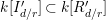 $k[I_{d/r}^{\prime }]\subset k[R_{d/r}^{\prime }]$
is birational. Now Corollary 5.8 and Remark 5.9 imply the asserted statements for the ideals
$k[I_{d/r}^{\prime }]\subset k[R_{d/r}^{\prime }]$
is birational. Now Corollary 5.8 and Remark 5.9 imply the asserted statements for the ideals
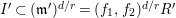 $I^{\prime }\subset (\mathfrak{m}^{\prime })^{d/r}=(f_{1},f_{2})^{d/r}R^{\prime }$
in
$I^{\prime }\subset (\mathfrak{m}^{\prime })^{d/r}=(f_{1},f_{2})^{d/r}R^{\prime }$
in
 $R^{\prime }$
. To pass back to the ideals
$R^{\prime }$
. To pass back to the ideals
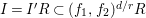 $I=I^{\prime }R\subset (f_{1},f_{2})^{d/r}R$
in
$I=I^{\prime }R\subset (f_{1},f_{2})^{d/r}R$
in
 $R$
we use the fact that the map
$R$
we use the fact that the map
 $R^{\prime }\subset R$
is flat with Gorenstein fibers. We remind the reader that
$R^{\prime }\subset R$
is flat with Gorenstein fibers. We remind the reader that
 $$\begin{eqnarray}\operatorname{core}(I)=\operatorname{core}(I^{\prime }R)=\operatorname{core}(I^{\prime })R,\end{eqnarray}$$
according to [Reference Polini, Ulrich and Vitulli45, 2.1] and [Reference Corso, Polini and Ulrich12, 4.8]. ◻
Remarkably, if
 $s=2$
then all the statements of Corollary 5.8 are equivalent. More specifically, the integral closedness of the core, which is a single graded component of the canonical module of the Rees ring, forces the shape of the entire canonical module.
$s=2$
then all the statements of Corollary 5.8 are equivalent. More specifically, the integral closedness of the core, which is a single graded component of the canonical module of the Rees ring, forces the shape of the entire canonical module.
Corollary 5.14. Adopt the data of 3.1. In addition assume that
 $I$
is
$I$
is
 $\mathfrak{m}$
-primary,
$\mathfrak{m}$
-primary,
 $s=2$
, and the field
$s=2$
, and the field
 $k$
is infinite. Statements (1)–(8) are equivalent.
$k$
is infinite. Statements (1)–(8) are equivalent.
-
(1) The morphism
$\unicode[STIX]{x1D6F9}$
is birational onto its image, that is
$[B:A]=1$
. -
(2) The Rees ring
${\mathcal{R}}(I)$
satisfies Serre’s condition
$(R_{1})$
. -
(3)
$\unicode[STIX]{x1D714}_{{\mathcal{R}}(I)}=\unicode[STIX]{x1D714}_{{\mathcal{R}}(\mathfrak{m}^{d})}$
. -
(4)
$\operatorname{End}_{{\mathcal{R}}(I)}(\unicode[STIX]{x1D714}_{{\mathcal{R}}(I)})=\operatorname{End}_{{\mathcal{R}}(\mathfrak{m}^{d})}(\unicode[STIX]{x1D714}_{{\mathcal{R}}(\mathfrak{m}^{d})})$
. -
(5)
$e(A)=d$
. -
(6)
$\text{core}(I)=\mathfrak{m}^{2d-1}$
. -
(7)
$\text{core}(I)=\text{adj}(I^{2})$
. -
(8) The ideal
$\text{core}(I)$
is integrally closed.Furthermore, statements (1)–(8) are all implied by
-
(9)
$\gcd \,(\mathit{column~degrees~of}\;\unicode[STIX]{x1D711})=1$
.


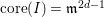


Proof. Corollary 5.8 shows that items (1)–(5) are equivalent and that they imply (6) and (7). Item (8) follows immediately from (6) or (7). We prove that (8) implies (1). From Theorem 5.13, we have
 $\text{core}(I)=(f_{1},f_{2})^{2(d/r)-1}$
. Hence
$\text{core}(I)=(f_{1},f_{2})^{2(d/r)-1}$
. Hence
 $\operatorname{core}(I)$
is an
$\operatorname{core}(I)$
is an
 $\mathfrak{m}$
-primary ideal generated by
$\mathfrak{m}$
-primary ideal generated by
 $2d/r$
forms of degree
$2d/r$
forms of degree
 $2d-r$
. If such an ideal is integrally closed, it would have to be
$2d-r$
. If such an ideal is integrally closed, it would have to be
 $\mathfrak{m}^{2d-r}$
, which is minimally generated by
$\mathfrak{m}^{2d-r}$
, which is minimally generated by
 $2d-r+1$
forms. This forces
$2d-r+1$
forms. This forces
 $r=1$
. Finally we appeal to Corollary 4.6(3) to see that (9) implies (1).◻
$r=1$
. Finally we appeal to Corollary 4.6(3) to see that (9) implies (1).◻
Remarks 5.15.
-
(a) If
$I$
is generated by monomials then statements (1)–(9) of Corollary 5.14 are all equivalent according to Observation 4.7. -
(b) When statements (1)–(8) of Corollary 5.14 hold, then it follows from Corollary 5.8 that all of the equalities
hold.
$$\begin{eqnarray}\text{gradedcore}(I)=\text{core}(I)=\text{core}(\mathfrak{m}^{d})=\mathfrak{m}^{2d-1}=\text{adj}(I^{2})\end{eqnarray}$$
-
(c) Kohlhaas [Reference Kohlhaas34] has proven that if
$I\subset k[x_{1},\ldots ,x_{s}]$
is an
$\mathfrak{m}$
-primary monomial ideal which has a reduction generated by
$s$
monomials, then the following three conditions are equivalent.(2)
$R[It]$
satisfies Serre’s condition
$R_{1}$
.(7)
$\operatorname{core}(I)=\text{adj}(I^{s})$
.(8)
$\operatorname{core}(I)$
is integrally closed.


Acknowledgments
This paper was written at Centre International de Rencontres Mathématiques (CIRM) in Luminy, France, while the authors participated in a Petit Groupe de Travail. The authors are very appreciative of the hospitality offered by the Société Mathématique de France.
