


Introduction
A wide variety of brain functions including cognition, verbal ability, and decision making are performed by the synergy of a huge number of neurons configured in a three-dimensional (3D) network in brain tissue. The first step to understanding how the brain functions is to analyze this 3D structure. Because neurons exert their functions by interacting with each other, a number of neurons should be visualized simultaneously to illustrate the functional mechanisms of the brain. Although structural studies of brain tissues have been reported, the structures of these tissues, which are composed of many neurons, are difficult to comprehend. This is because there is a lack of quantitative descriptions of neuronal networks, which should be represented with 3D Cartesian coordinates, rather than a 3D distribution of intensities.
This article reports the structures of brain tissues belonging to humans [Reference Mizutani1] and the fruit fly Drosophila melanogaster [Reference Mizutani2] that were ascertained using X-ray tomographic microscopy, a microscopic version of medical computed tomography (CT). In order to analyze the brain network, the structure of each neuron should be described in terms of 3D Cartesian coordinates by building skeletonized models of neurons. The structural components of the fly brain network were classified on the basis of their 3D structures. This classified model allowed identification of anatomical segments. The network of human brain tissue indicated that the neurons form feedback loops. Such feedback loops can be viewed as canonical elements in brain circuits.
Materials and Methods
Contrasting brain tissues
The transparency of biological tissue to hard X rays enables radiographic analysis of tissue structures. Soft tissues are composed of light elements, which produce little contrast in a hard X-ray image. In clinical diagnosis, luminal structures of a living body are visualized by using X-ray contrast media. These contrast media contain high-atomic-number (high-Z) elements that attenuate X rays efficiently. Tissue-staining methods using high-Z elements, such as Golgi impregnation and reduced-silver impregnation, are known as conventional techniques for the histology of brain tissues. In this study, the tissue structures were visualized with these impregnation methods.
Post-mortem human cerebral tissues were collected with informed consent from the legal next of kin using protocols approved by ethical committees of organizations related to this study. The frontal cortex tissues were subjected to Golgi impregnation, as described previously [Reference Mizutani1]. Neurons were visualized with silver deposits in dendrites, axons, and cell bodies with this method.
Wild-type fruit flies Drosophila melanogaster Canton-S (Drosophila Genetic Resource Center, Kyoto Institute of Technology, Japan) were raised on standard cornmeal-molasses fly food and kept at 20°C. Adult fly brains, also referred to as the cephalic ganglion, were dissected and subjected to modified reduced-silver impregnation, as described previously [Reference Mizutani2]. It has been shown that neurons were visualized with metal gold particles derived from the aurate toning reagent used in this method.
Tissue embedding
Tissue structures should be kept constant during the data collection. However, biological soft tissues themselves are not rigid and show deformations depending on ambient conditions. Therefore, the tissue samples were embedded in epoxy resin [Reference Mizutani1, Reference Mizutani2] as one would do in the case of transmission electron microscopy.
Resin embedding was performed by transferring the tissue sample from an aqueous solution to first ethanol, then to n-butyl glycidyl ether, and finally to the resin. In the case of embedding a block sample with dimensions of 5 × 5 × 5 mm3, the tissue was soaked in 10 mL of 100% EtOH for a few hours or overnight at room temperature (20–25°C). This process was repeated three times in total. The tissue was then transferred to 10 mL of n-buthyl glycigylether and left for several hours or overnight at room temperature. This process was repeated twice in total. Subsequently, the tissue was soaked in a 2 mL aliquot of Petropoxy 154 (Burnham Petrographics, ID) epoxy resin overnight at 4°C. The epoxy resin was degassed prior to use. This process was repeated twice in total. If the tissue floated to the surface of the resin even after two cycles of resin soaking, an additional soaking using another resin aliquot was performed.
Human brain tissues soaked in the resin were cut into rod shapes with widths of 0.3–0.5 mm under a stereomicroscope and transferred to a borosilicate glass capillary (W. Mìller, Germany) filled with the resin. Larger tissue samples with widths of 1.5–3 mm were also prepared and embedded in resin pellets. The fly brain was embedded in a tiny resin drop using a nylon loop for protein crystallography (Hampton Research, CA). The samples were then kept at 90°C for 40–90 hr for curing the resin.
Sample mounting
The resin-embedded samples were mounted on the sample stage using brass fittings (Figure 1a). Example samples are shown in Figure 1b. Pellet samples were attached to the flat surface of the brass fitting using epoxy glue or double-stick tape. Epoxy glue is preferable for high-resolution analysis. Capillary samples with outer diameters greater than 0.5 mm were inserted in clay stuffed in a hole made at the end of the brass fitting. Because the capillary insertion compresses the residual air in the hole and its re-expansion can cause sample drift during data collection, a minuscule side opening was made in the lateral face of the fitting (Figure 1c) to vent the air and clay. Capillaries with diameters less than 0.5 mm were sleeved with a brass tube using epoxy glue and secured with a setscrew. Sample mounting was finished at least 30 minutes before the data collection to stabilize the samples. For tomographic microscopy with resolutions higher than 200 nm, the mounted samples should be placed near the sample stage as soon as possible in order to equilibrate their temperature with that of the apparatus.

Figure 1 (a) X-ray tomographic microscopy at BL20XU of SPring-8. The incident X-ray beam comes from the left, and transmission images were acquired with the detector. (b) Samples for tomographic microscopy. Pellet sample (labeled A) was attached to the flat surface of the brass fitting using double-stick tape B. Capillary sample C was inserted in clay stuffed in a hole of brass fitting D. Clay ejected from a side opening can be seen. Capillary sample E sleeved with a brass tube F was fixed using a wrench G. (c) Schematic drawing of the upper end of the fitting D. An opening with a diameter of 0.5 mm was made for venting air and clay under pressure in the hole.
Tomographic microscopy
Simple-projection tomographic microscopy was performed at the BL20XU beamline of the SPring-8 synchrotron radiation facility, as reported previously [Reference Mizutani1]. X-ray tomographic microscopy with Fresnel zone plate (FZP) optics was performed at the BL37XU and BL47XU beamlines. In the BL37XU experiment, a FZP with an outermost zone width of 100 nm and diameter of 310 µm was used as an X-ray objective lens to visualize structures at 160–200 nm resolution. In the BL47XU experiment, a FZP with an outermost zone width of 100 nm and diameter of 774 µm was used as an X-ray objective lens to take images with a viewing field wider than 500 µm. Transmission images were recorded with a CMOS-based imaging detector (Hamamatsu Photonics, Japan). The data acquisition conditions are summarized in Table 1.
Table 1 X-ray tomographic microscopy data collection conditions.
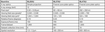
a Width × height
X-ray images were subjected to a convolution back-projection calculation using the RecView program (available from http://www.el.u-tokai.ac.jp/ryuta/). The obtained tomographic cross sections were stacked in order to reconstruct a 3D image of the sample. Spatial resolution was estimated with 3D square-wave patterns [Reference Mizutani3].
Network analysis
In order to analyze the brain network, the structure of each neuron should be described by building a skeletonized model in the 3D image. The model was built by using a method like those used in crystallographic studies of macromolecular structures [Reference Mizutani1]. Because it takes considerable person-hours to manually build models of neuronal networks, an initial model was automatically built by machine interpretation of the 3D image [Reference Mizutani1, Reference Mizutani2]. First, large structures, such as cell body somas and blood vessels, were scanned to mask those regions from the subsequent tracing procedure. Cartesian coordinates of the large structures were also used for locating neuronal somas. Next, fibriform structures corresponding to dendrites and axons were searched by evaluating the gradient vector flow. The resultant coordinates with high fibriform scores were used as starting points to trace the neuronal processes using a Sobel filter [Reference Mizutani1]. This procedure was implemented with dedicated software to build models automatically [Reference Mizutani1, Reference Mizutani2]. The models obtained were manually examined and edited so as to assemble neuronal processes as neurons or to classify them into 3D structural groups.
Results
Fly brain network
Figure 2a shows the 3D structure of the fruit fly brain visualized at the BL37XU beamline. The spatial resolution of this image was estimated to be 160–200 nm. Neuronal processes were clearly visualized as network structures. In order to analyze the overall network, a skeletonized model was built using a 3D image obtained at BL47XU (Figure 2b). The obtained model consists of neuronal processes with a total length of 378 mm in a volume of 0.220 × 0.328 × 0.314 mm3.

Figure 2 (a) Three-dimensional rendering of the network of the fruit fly brain. The structures including the midline component called the central complex are illustrated. Scale bar = 10 µm. (b) Skeletonized model of the left hemisphere is superposed on the entire brain structure. The front side of the rendering is cut off to show inner structures. Scale bar = 20 µm. CB, central brain; OL, optic lobe.
The network constituents were classified into groups on the basis of their 3D structures [Reference Mizutani2]. The classified model (Figure 3) allowed us to extract anatomical segments by specifying neuronal processes in a group-by-group manner. For example, the lobula plate (Figure 3e) located at the posterior end of the optic lobe can be distinguished from the other structures by its location and structures specific to the lobula plate. Neurons of the lobula plate were characterized by their fan-shaped ramification. Such structures of the lobula plate can be extracted from the model by specifying corresponding structural groups.

Figure 3 Skeletonized model of the left hemisphere of the fruit fly brain. The entire model (a) can be divided into CB and OL regions. The upper panel of (a) shows a side view with dorsal side toward the top. The lower panel of (a) shows a front view of the left hemisphere with the dorsal side toward the top The OL (b) can be further divided into the second optic chiasma (c), medulla (d), lobula plate (e), and lobula (f). Structural groups are color-coded. Scale bar=20 µm.
Figures 3b–3f show the organization of the optic lobe network, which is responsible for visual information processing. Neuronal processes of the medulla and second optic chiasma, which are proximal to the compound eye, exhibit periodical structures corresponding to repeated units of photoreceptors. On the opposite side of the optic lobe, neuronal processes are assembled into several tracts pointed toward central brain regions. These structures represent information paths from the inputs on the eye to the integrative process in the central brain. Refinements of these models by using the high-resolution data should reveal finer 3D aspects of the fly brain.
Human brain circuits
Figures 4 and 5 show the structures in the human frontal cortex tissues. The 3D images of a block sample with dimensions of 1.4 mm×1.4 mm×8.3 mm are so complicated (Figure 4) that they cannot be comprehended at a glance, although pyramidal neurons arranged in a soma layer, called the internal pyramidal layer, can be seen in the image. A smaller sample with dimensions of 0.30 mm×0.35 mm×2.4 mm was also visualized with tomographic microscopy and subjected to model building. Skeletonized models of neurons (Figure 5a) were built by tracing the neuronal processes and assembling them into neurons. Although it is still difficult to comprehend the entire models, any of the neurons composing them can be extracted (Figure 5b). Because the models are described in terms of 3D Cartesian coordinates, the distances between the neuronal processes or somas can be directly calculated from the coordinates. This enabled us to determine individual neuronal circuits by analyzing the positional relationships of the neurons [Reference Mizutani1]. The pair of neurons shown in Figure 5b connect their inputs and outputs to each other to form a feedback loop (Figure 5c). In electronics, a similar feedback circuit composed of transistors is known as an astable multivibrator (Figure 5d), which generates a string of pulses. The refractory period of neurons prevents repetitive action potentials and hence poses a limit on the firing interval. However, a delay through a loop composed of a number of neurons allows recovery from the refractory period of a few milliseconds, resulting in oscillations of the loop circuit. Because such feedback loops are formed if a number of neurons are connected to each other, the loop circuit should be one of the canonical structures of human brain circuits.

Figure 4 Three-dimensional structure of human frontal cortex tissue. X-ray linear attenuation coefficients were rendered from 9 cm-1 (white) to 112 cm-1 (black). Arrowheads indicate the internal pyramidal layer. Scale bar = 100 µm.

Figure 5 (a) Skeletonized model of a neuronal network of the human frontal cortex. The brain surface is toward the top. Soma positions are indicated with closed circles. Neurons are color-coded. Total width: 240 µm. (b) A pair of neurons 1020 (magenta) and 1023 (green) were extracted from the model. Possible synaptic connections are indicated with black dots. (c) Neurons 1020 and 1023 connect their inputs and outputs to each other to form a feedback loop. Dendrites are drawn with thin lines, and axons with arrows. Possible synaptic connections are indicated with diamonds. Reprinted with permission from [5]. (d) A similar feedback circuit composed of transistors is known as an astable multivibrator.
Discussion
Three-dimensional structures of neuronal networks of human and fruits fly brains were visualized with X-ray tomographic microscopy [Reference Mizutani1, Reference Mizutani2]. The obtained structures were analyzed by building skeletonized models of neurons. This quantitative description of 3D networks in Cartesian coordinate space enabled examination of the functional mechanisms of the obtained brain networks.
The functional architecture of the visual cortexes of cat and monkey brains has been incorporated into artificial neural networks [Reference Bengio4]. This neural network, called a convolutional neural network, has been applied to image recognition tasks and has outperformed other computing methods designed without reference to the visual cortex architecture [Reference Bengio4]. The present study illustrated some of the circuits of the human frontal cortex, which is responsible for higher brain functions. These circuits should provide a basis for cognitive computing to deal with complicated problems that have not been able to be handled without human intervention.
The psychological individuality of human beings is ascribable to the individuality of their brains. Therefore, psychological characters reside in the neuronal circuits of the brain. Differences between neuronal circuits should be observable not only in healthy individuals, but also between patients with brain disorders and healthy controls. Such differences can be clues to improving the treatments of brain disorders. Because our knowledge of the circuits in the human brain is still limited, drugs for treating brain disorders are being administrated without a complete understanding of their mechanisms of action on the circuits of the brain. Better diagnosis, prevention, and treatment of brain disorders should thus be possible by analyzing brain networks and identifying neuronal circuits responsible for individual brain disorders.
Conclusion
Neurons make up a 3D network in brain tissue. This article reports on the 3D structures in human and fruit fly brain tissues as measured with a microscopic version of medical computed tomography (CT) called X-ray tomographic microscopy (or microtomography or micro-CT). The obtained structures were analyzed by building skeletonized models of neurons. The resulting quantitative description of the 3D networks provided information about the functional mechanisms of the brain.
Acknowledgments
This work was supported in part by Grants-in-Aid for Scientific Research from the Japan Society for the Promotion of Science (nos. 25282250 and 25610126). The synchrotron radiation experiments were performed at SPring-8 with the approval of the Japan Synchrotron Radiation Research Institute (JASRI) (proposal nos. 2008B1261, 2013B0034, 2013B0041, 2014B1083, 2014B1096, and 2015A1160).


