Introduction
For decades, fluorescence microscopy has been an invaluable tool in life sciences research, with new variations and implementations emerging almost every year. Laser scanning microscopy, airyscanning, structured illumination, light field and light sheet microscopy are among the many methods that have been developed through the years to overcome the limitations of the original widefield (WF) microscopy setups. These more recent techniques have brought new insights into biological samples and enabled new discoveries. However, we should not forget that even comparably simple and inexpensive WF microscopes can help to extract meaningful data from many samples. In this article we focus on some popular image processing methods. These techniques have the potential to make WF microscope systems more powerful and versatile so long as their limitations and pitfalls are known. Simple deblurring methods such as background subtraction, computational clearing, unsharp masking, and the like deliver a quick and clearer preview of the sample, while more accurate deconvolution models yield higher resolution, fewer artifacts, and more quantitative results.
Limitations of Widefield Microscopy
The most obvious limitation of WF fluorescence microscopy is the out-of-focus blur in the image that essentially limits contrast and prevents clear identification of structures and objects of interest. In a WF microscope, a beam of light simultaneously illuminates the whole field-of-view to excite all the fluorophores it contains. The beauty of this approach is that all parts of the specimen are viewed simultaneously, and the image can be captured simply and rapidly with a camera. However, due to diffraction-limited optics and the projection of out-of-focus light onto the camera-sensor, this usually results in images of low contrast, especially with thicker and more densely labeled specimens. Optical sectioning methods, such as confocal laser scanning microscopy (CLSM) or structured illumination microscopy (SIM), exclude out-of-focus light from the image and thereby will typically show better contrast and reveal more details (Figure 1).
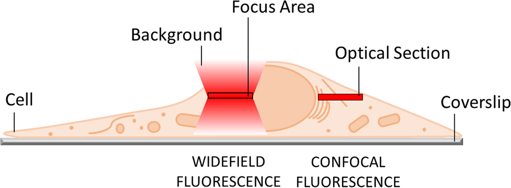
Figure 1: In WF microscopy (left) the captured image contains light from the focus area as well as significant background signal from out-of-focus areas above and below the focal plane. Confocal techniques (right) can employ various means to avoid this background contribution and thereby generate an image with better contrast.
Using a WF setup typically does the job for thin specimens, for example, layers of single cells or isolated organelles. When the signal is sparse and the objects are thin, the resulting WF images can reveal as much information as those captured with costlier, more highly sophisticated equipment (Figure 2). On the other hand, most WF microscopes cannot image thick tissues, 3D cell culture, spheroids, or whole organisms with sufficient contrast. These samples significantly scatter the light, and multiple layers of fluorescent structures make it hard to distinguish details in a 3D volume.

Figure 2: Figure 2A shows a WF image of cultured flat epithelial cells (actin filaments in green, mitochondria in purple) of a rat kidney. This comparison depicts the challenges posed to a WF instrument by a thick and scattering sample like the rat kidney (2B).
Solutions for 3D Volumes
Figure 1 shows the situation that occurs when only a single image of the sample is recorded. There are multiple possibilities when a 3D volume is sought. Optical sectioning techniques can be used to generate a stack of images that can then be rendered into a 3D object (Figure 3). For WF instruments, a technique called deconvolution has been available in microscopy for more than 20 years. In contrast to the early-2000s, today's deconvolution programs and microscopes produce results almost instantaneously, as GPU-based processing with the latest computer hardware accelerates the computation tremendously. Deconvolution microscopy is one of the best-described processing methods in the microscopical sciences and is based on mathematical models that aim to reverse the distortions that take place in optical instruments. There are numerous variants of deconvolution algorithms, and they all come with their own advantages and disadvantages, essentially differing in reconstruction quality and speed. Since there is not one perfect method for all image conditions, ZEN imaging software implements know-how from more than 20 published deconvolution variants to deliver best user experience and valid results at all times. A major benefit of the WF deconvolution approach is that no light from the sample is excluded during image acquisition; the maximum number of photons are collected and later reassigned to their real places of origin. This reveals many structures in the resulting 3D volume that were not visible before and so were lost in the out-of-focus light. Deconvolution microscopy is therefore also known as a signal-inclusive method.
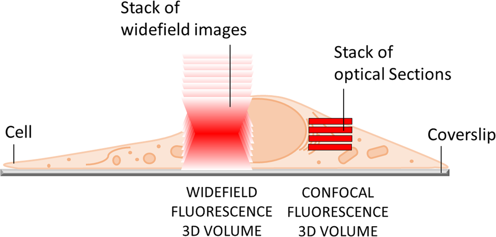
Figure 3: Acquisition of a WF image z-stack (left) supports processing by deconvolution to reconstruct a 3D volume as opposed to a 3D object creation with an optical sectioning approach (right).
Notably, it might take a bit longer to acquire a single optical section with SIM or CLSM than it does with a WF image. For example, SIM requires at least three images per section to be acquired, and a single point scanning confocal laser scanning approach requires point-by-point scanning, usually making it slower than simply snapping a camera image.
It is important to note that the deconvolution of WF images must not be regarded as a replacement for an optical sectioning system. Instead, any micrograph collected with a light microscope will benefit from deconvolution, including optical sections (for example, from laser scanning confocals, spinning disk confocals, or structured illumination images). So long as the right mathematical model is used, deconvolution will always help restore the photon signal to the exact place where it belongs (Figure 4), and this will increase contrast and resolution. Of course, one side effect in the case of WF images is that the out-of-focus blur disappears. When deciding which method to choose, there are many aspects to consider if a 3D volume is ultimately needed. These range from the desired time and spatial resolution to spectral flexibility, penetration depth, and various other factors (Table 1).

Figure 4: Mitochondrial membranes labeled with TOMM22, acquired with a ZEISS LSM system using fast linear scanning (left). The top row shows a single plane of the dataset displayed before (left) and after the image was processed with a constrained iterative deconvolution in ZEISS ZEN imaging software, revealing additional details and increasing the resolution (right). The bottom row shows a detail of the yellow inset region and the improved image quality following deconvolution.
Table 1: Factors that must be considered when collecting 3D volume data and using deconvolution.

Sharp Images in 2D
What do you do when all you need is a crisp 2D image; whether in the form of a time series or as a large tiled image of a sample? As illustrated in Figure 2, very flat objects usually continue to reveal their biology quite well with a WF image. Still, there will be a certain background fluorescence that negatively influences the aesthetic aspects and contrast. The human eye likes crisp details along with sharp contrast and colors. A first and really quite simple way to make a fluorescence image look more appealing and reveal some additional details is to adjust the display curve in the software. So long as an image is not exported as a TIF or JPG image, this will not in itself change the image data but will only influence the look of the image on the screen. As out-of-focus haze in WF images is typically less intense than the in-focus structures, this approach can work to a certain extent. However, it fails where in- and out-of-focus structures are lying on top of each other, and it is also quite an arbitrary procedure that depends ultimately on the operator's preferences. Therefore, more powerful methods are usually called for.
Over the past few decades, numerous processing methods have been developed for delivering crisper, sharper images. These procedures have several primary goals, for example, to remove shading, improve contrast, remove blur, or enhance certain structures—all, of course, with the ultimate goal of making the image more suitable for inspection or presentation. However, before applying these methods to micrographs, first consider the impact they will have on the image itself. Many post-processing steps introduce noise (to a varying degree) to the image, and simple post-processing steps can never increase its information content. Nevertheless, a processing step might be exactly what is needed to make the information and details that are present in an image more apparent, or just to make it more appealing visually. Let's look at some of the most commonly used processing methods. These could be categorized as “deblurring” methods, and they all have one thing in common: unlike deconvolution, they work on one image after another without including any 3D volume information or a mathematical model of the distortions generated in the instrument that acquired them.
Unsharp Masking
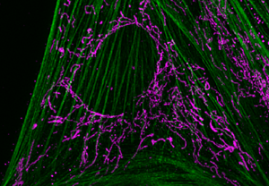
Figure 5 shows detail from the cells seen in Figure 2 and illustrates what a relatively simple procedure called “edge detection” can do to any WF fluorescence image. On the left is the raw, unprocessed region of interest (ROI). On the right, the same ROI is shown after a single processing step using the unsharp masking method, introduced by Russ in 1994 [Reference Russ1]. The effect is quite impressive and, at first sight, the unprocessed image might even look a bit out of focus next to the much sharper, processed image. This impression is a result of humans being hard-wired to look for sharp edges and lines and to consider these to be more detail-rich than fuzzier representations of the same image. Unsharp masking is like many post-processing methods in that it will not add to, but instead will reduce the information content of the image. The loss of information is easily understood if we look at the way this sharpening is achieved. The algorithm subtracts an unsharp mask from the specimen image. The mask is simply an artificially blurred image that is produced by applying a Gaussian low-pass filter to the original image. Consequently, this procedure inevitably increases noise in the image. Nevertheless, edge-enhancing methods do a good job in making geometrical structures stand out more prominently, especially for thin and transparent objects like 2D cell cultures. As a free bonus, the unsharp mask filter also suppresses low-frequency details and can be used to correct shading throughout an image. This is often visible in the form of slowly varying background intensities.

Figure 5: Unprocessed WF image of a cell (left) and the same image processed with unsharp masking (right). Actin filaments in green, mitochondria in purple.
No-Neighbor/Nearest-Neighbors
These two processing methods are sometimes classified as deconvolution methods. However, although the nearest-neighbors method in particular shares some characteristics with real 3D deconvolution procedures, both processing methods are filters designed to subtract the estimated blur from the image. The early concept was introduced to light microscopy by Castleman in 1979 [Reference Castleman2] and first applied practically by Agard in 1984 [Reference Agard3]. The no-neighbor method achieves deblurring by looking only at the image itself, whereas the nearest-neighbors method also takes into account information from one plane above and one below, which means a z-stack must be acquired. The nearest-neighbors method attempts to remove the blur contribution in the center focal plane by subtracting defocused versions of the adjacent slices including knowledge of the point spread function (PSF), and this leaves only sharp features behind. The no-neighbor method is similar although it only considers a single slice. It is therefore equivalent in principle to an unsharp masking, which we have already discussed. On the positive side, both methods require very little computing power and are fast (virtually executed in real-time), but they are also very limited in their capabilities and often mishandle blurred light. They also reduce signal intensities (usually around 50 to 90%) across the image and should only be used for a quick check of the image when, for example, further optimization of the image acquisition parameters is necessary.
Background Subtraction
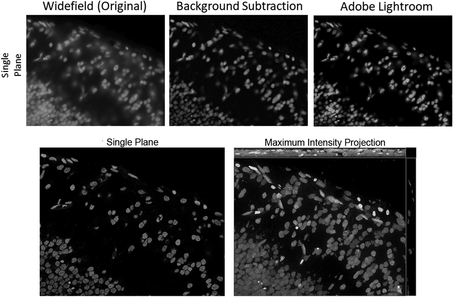
This is a very effective way to increase contrast in WF images, offering many possibilities for improving a WF image by using image and computational processing to reduce the background. One method that has been around for a very long time is the so-called rolling ball background subtraction algorithm. This was inspired by Stanley Sternberg's article, “Biomedical Image Processing” in IEEE Computer [Reference Sternberg4]. It removes continuous or uneven background from images by determining a local background value for every pixel, averaged over a very large ball around the pixel. The value is thereafter subtracted from the original image. Thus, the most important parameter is the rolling ball radius, which should be at least as large as the radius of the largest object that is not part of the background. It is quite easy to estimate the parameter when the magnification of the system is known, but it can never be accurate when the sample types change or the structures in them are uncommon. The so-called instant computational clearing (ICC) used in products of Leica Microsystems marketed as “Thunder™ Imager”, is based on the principle of separating out the background and subtracting it from the image. No-neighbor and rolling-ball methods, as well as ICC, employ filter algorithms to identify and remove image content that is likely to be caused by out-of-focus blur. This removal can also be preceded by a nearest-neighbors deblurring to eliminate even more “blurry” structures. Figure 6 shows fluorescently labeled nuclei acquired with an inverted WF setup. The original WF image has then been processed to clear the haze from the image by either a background subtraction based on the rolling ball algorithm (as implemented in ZEISS ZEN imaging software) or by a series of image processing steps available in the Adobe Lightroom® photo processing software.

Figure 6: Top row: Grayscale images of fluorescently labeled nuclei. Out-of-focus blur is visible in the original WF image (left), as there are multiple layers of nuclei above and below the focus plane. Rolling ball background subtraction was carried out with the original WF image in ZEISS ZEN lite (middle), eliminating most of the haze in the image. A series of adjustments (90% dehaze, 80% clarity, 80% texture, 80% blacks, 10% contrast) to the original WF image have been made with the software Adobe Lightroom® (right), resulting in a very similar elimination of haze, as compared to the background subtracted image in the middle. Bottom row: As a gold standard, the same image plane with a maximum intensity projection is shown, based on a stack of optical sections acquired with a ZEISS Apotome.2.
As seen in Figures 7 and 8, simple background subtraction leads to removal of the haze in the images but does not reveal all fine details in them. Also, the resolution of the image is not enhanced by the background subtraction. This becomes especially apparent when the same image is not only compared to a WF image, but also to one that has been acquired or processed with more advanced techniques, such as 3D deconvolution and/or optical sectioning methods. One further problem that is sometimes seen with background subtraction, especially with the rolling ball method, is an overrepresentation of faint spots in the resulting image, as well as box-like artifacts. To reduce this, several modifications to the rolling ball algorithm have been made; for example, the floating ball (Bio-Rad) method is a modification of a combination of fuzzy and rough set theories [Reference Huang5]. In addition, many efforts have been made to subsequently remove artifacts from images that are caused by rolling ball and lowpass filtering [Reference Cai and Verbeek6].

Figure 7: Single-plane and maximum-intensity (ortho) projections of a WF image of a polychaete worm are stained in green and red (left). The image stack was processed with a rolling ball background subtraction in ZEISS ZEN lite, and the result is shown in the middle. Compared to the WF image, more structures are visible in the background subtracted dataset, but many details are missing in relation to the images acquired by optical sectioning with an Apotome.2 (right). In addition, some of the compact green structure on the edges seems to have eroded. Image stack height: 160 µm, 400 planes.

Figure 8: 3D rendering of a z-stack of a zebrafish, stained in blue, green, and red (left). The image stack was processed with a rolling ball background subtraction in ZEISS ZEN lite, and the result is shown in the middle. Compared to the WF image, more structures are visible in the background subtracted dataset, but many of the details are missing in relation to the images acquired with the Apotome.2 (right). Image stack height: 120 µm, 80 planes.
No matter how much these techniques are improved, their general hallmark and working principle is signal exclusion, essentially based on feature size. This can lead to artifact generation and loss of information. A good example of lost signal is the “hole” in the inner parts of larger organisms or spheroids that is generated by background correction or computational clearing. The homogeneous fluorescence in the inner part has properties similar to the homogeneous blur of out-of-focus light, and it is therefore “removed” (Figure 9). Another example on a smaller scale is shown in Figure 10. Deconvolution reproduces the very crisp structures of mitochondria and microtubules while also showing the mitochondrial membrane stains. It also shows quite well the nucleolar-like structures that are hardly visible in the cell nucleus. This weak signal is eroded and entirely removed by background correction, and the information is lost. In addition, all background correction methods change the signal-to-background ratio, which means that the results of an x-fold increase in a fluorescence response after background subtraction must not be directly compared to an x-fold response in an image without background subtraction applied. Figure 11 depicts the changes in intensities compared to a WF image after undergoing either background correction, deblurring (nearest-neighbors), or a full 3D deconvolution. As far as we can tell, the overall profile looks similar, but the advantages of reassigning photons from an entire z-stack to a 3D deconvolution over simply removing the background are quite obvious. Meanwhile, processing times are very small, even for 3D deconvolution, the most sophisticated method.

Figure 9: Giant liver fluke stained with Hoechst 33342. The homogeneous fluorescence in the inner parts of the WF image (left) poses a serious problem for background correction algorithms (center). Some structures remain, but generally there are too many black spaces between the cells. This becomes visible when comparing the results to an optical section, acquired with ZEISS Apotome.2 (right). Notably, the prominent rim around the structure, as seen by the background corrected image in the center panel, is an artifact of interference in the WF image, which is not seen with an optical sectioning system.

Figure 10: Overview and two regions of interest of a z-stack of cells (mitochondria in green, EB3 microtubule tips in red) acquired with a WF setup (left). Center: Background subtracted dataset from the left image. Right: 3D deconvolved dataset from the left image (constrained iterative method in ZEISS ZEN imaging software). In the overview, background subtracted and deconvolved datasets look very similar, but differences become visible in the detailed regions of interest. In Detail 2, it becomes apparent that the spatial resolution of the deconvolved dataset is much better compared to the background corrected image. In Detail 1, structures that are visible in the WF image can also be observed in the deconvolved image stack, but not with the background subtracted data, no matter how much the display contrast and brightness are increased.

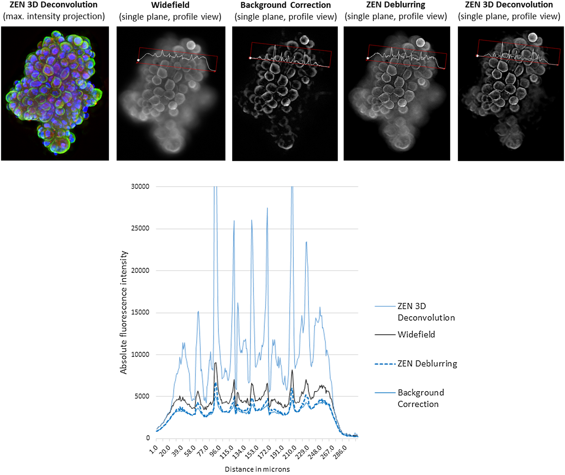
Figure 11: A z-stack of tumor spheroids (height: 100 µm) was acquired with ZEISS Celldiscoverer 7 and a 5×/0.35 objective with 2 × tube lens. Nuclear counterstain (blue), and green and red fluorescence. Top: From left to right: maximum intensity projection of 3-color fluorescence image after constrained Iterative deconvolution in ZEISS ZEN; single plane of a WF stack (green channel) with profile line; single plane of a WF stack, background corrected with the rolling ball method; single plane of a WF stack, deblurred using nearest-neighbors method in ZEISS ZEN; single plane of a WF stack, deconvolved using constrained iterative method in ZEISS ZEN. Approximate processing times of full 3-channel z-stack (relative values): BG-correction (<1 sec), deblurring (1 sec), deconvolution (~10 sec). Bottom: Intensity values of profile lines shown for all four processed images. Image courtesy of R. Buschow, Max Planck Institute for Molecular Genetics, Berlin.
Deblurring and background subtractions (using the rolling ball or nearest-neighbors method, or other approaches) usually do a good job in improving threshold-based segmentation of images because they render the background even and remove blur around objects. Therefore, they play a valuable part in image analysis workflows. However, when using them to reveal and extract information from images in order to draw scientific conclusions from them, they should be complemented by an approach that models the 3D context of a sample (Table 2).
Table 2: Typical suitability (relative to each other in terms of effort and quality) of clearing methods for WF images. More points mean better suitability.

* Apotome-like structured illumination, single- or multi-point laser scanning.
** For example, cell counting, nuclei or whole cell segmentation, area measurements.
*** For example, co-localization analysis, 3D particle tracking, protein fine localization, intensity measurements.
Conclusion
Confocal laser scanning microscopy or structured illumination methods (Apotome) use a sophisticated optical setup to allow acquisition of sharp images from single planes and of entire 3D volumes. 3D deconvolution approaches take into account as much information as possible from the imaging system and the sample in order to reconstruct the 3D volume as accurately as possible. Typical post-processing methods such as background subtraction and unsharp masking, by way of contrast, are carried out in ignorance of how the image was acquired, what the properties of the imaging instruments were, and what the sample type was. This inevitably leads to a loss of information, even if the image looks improved to the naked eye, especially if assumptions about diameter or size of structures in an image are false; then such processing steps will yield incorrect results. In addition, these methods are all “exclusive,” which is to say they exclude photons from above and below the focal plane since they only take a single image into account. This exclusivity prevents their benefiting from the majority of photons in a 3D volume. In contrast to this, 3D deconvolution (as a “single-inclusive” method) will result in high signal-to-noise and better contrast and resolution as a result of reassignment of photons from other planes to the current focal plane.