


Introduction
Transmission electron microscopy (TEM) is widely used for resolving the ultrastructures of biological samples, materials, and hybrid soft/hard systems. Recent advances in sample preservation and microscope hardware have dramatically increased imaging throughput and have enabled access to higher statistical power for biological studies. As more samples can be examined within a fixed time, the challenge associated with data processing also increases. Image processing is becoming a significant component of modern microscopy projects, particularly as a required step in image analysis. Surprisingly, one of the most labor-intensive tasks in electron micrograph processing for biological samples involves the separation of the various cellular organelles, such as the nucleus, mitochondria, Golgi, etc. In order to investigate the linkage between ultrastructure and higher-order cellular function, the organelles must first be “selected” or segmented from the cellular background. For example, a common analysis to understand the connection between chromatin topology and gene transcription involves comparing EM images of nucleus texture from normal cells and cancer cells [Reference Garma1].
Usually, manual nucleus segmentation is important for determining correct statistical relationships (for example, not impacted by imprecision and random fluctuations within the cellular membrane space surrounding the organelle). As modern microscopy offers easy access to large datasets, image acquisition is no longer the bottleneck for biological studies, but labor-intensive manual image segmentation is. Moreover, humans are prone to bias and inconsistencies, which might also render the downstream statistical analysis unreliable. Therefore, an accurate, automatic, and consistent computational tool for image segmentation should be useful to accelerate biological research. This article describes such an automation tool.
Automated Segmentation
Image segmentation using neural networks
To meet this end, machine learning can provide a potential solution for “labeling” EM images by automating the segmentation process after observing a set of “ground truth” hand-processed examples. “Labeling” is classifying the data, or in the case of this study, segmenting the image. This approach has already found use in critical applications as disparate as self-driving cars and segmenting diagnostic features in patients’ medical CT scans [Reference Zheng2]. Supervised machine learning methods, such as deep learning, on the other hand, rely on inferring a common pattern from a set of “perfect” or “ideal” ground truth examples [Reference Coates, Ng and Montavon3]. This would be “learning by example.”
In the present work, a class of deep learning methods, known as convolutional neural networks (CNNs), is used for image segmentation. A CNN contains a large set of matrices that are iteratively convolved with the input data, typically an image. A convolution is a specific matrix operation that can reduce an image to features of interest. Initially, the convolutional matrices in a CNN are populated by random numbers, such that input images are randomly transformed and distorted. By comparing the output of the network against the desired output, values inside the network can be optimized using the chain rule, a calculus technique for optimization. Minimizing the error at the end of the process using a differentiable loss function results in a set of parameters that can perform a complex task, such as image segmentation.
Optimizing the CNN with training data
A CNN can have millions or tens of millions of individual parameters that must be optimized, or tuned, using input/output pairs, which are the labeled data pairs that the model learns from. A lack of labeled data can result in overfitting the data, when the algorithm becomes overly focused on details that are specific to the small set of images in the training. In all cases, the generalizability (or the quality of predictions on unseen data) of a CNN is directly dependent on the overall size and quality of the training data [Reference Pinto4]. Most computer vision tasks leveraging CNNs require thousands to millions of labeled data pairs, as in the case of PASCAL VOC 2011 [Reference Everingham5] and ImageNet [Reference Deng6]. For biological EM, analyzing and processing the raw data often involves expert knowledge and a significant amount of time, so hand-labeling tens of thousands of images as training data is likely prohibitive. Thus, although the idea of using CNN for image segmentation has been around for several years, implementation of it remains challenging.
Smaller training sets
Many efforts have been made toward generalizing CNNs with a small training set. Among them, data augmentation has been effective for several types of biological samples [Reference Ronneberg7]. In data augmentation, a small set of input/output pairs are artificially altered through simple geometric transformations to create new entries. These transformations include rotations, scaling, translations, and elastic deformations, among others. In addition to data augmentation, smaller models with fewer parameters based on encoder-decoder structures, such as the U-Net CNN architecture, also have been successful in segmenting biological samples from differential interference contrast (DIC) and electron microscope images with few training examples [Reference Ronneberg7]. Encoder-decoder structures entail downsizing the image to the features of interest and then restoring the image with its low-level features. By combining data augmentation with the U-Net model, a hybrid algorithm has achieved unprecedented success in certain tasks. In some cases, the algorithm can work with only 15 training examples [Reference Ronneberg7].
Connecting new data with the training set
Further enhancements on the basic CNN structure have relied on changing the way convolutions and nonlinear activations are arranged. Residual blocks (resblocks) are one way to connect the convolution operations between the input and output. The residual block structure allows the network to learn small features rather than full image transformations, thus making it easier to pass errors back through the network during training [Reference He8]. The Deep ResUnet model, also known as Deep Residual U-Net, implements residual blocks to increase training speed and simultaneously reduce the risk of overfitting [Reference Zhang9]. With 15 convolutional layers, 6 residual blocks, and no data augmentation, ResUnet has a record performance of 98.66% accuracy on the Massachusetts roads dataset [Reference Zhang9].
Testing the model with TEM images
This article examines the effectiveness of a Deep ResUnet model for segmenting TEM images of stained nuclei from human cheek cells. The effectiveness of data augmentation has been examined by varying the training data size for a generalizable model.
Materials and Methods
TEM sample preparation
Human cheek cells were harvested using a Cytobrush® (CooperSurgical, Trumbull, CT) by gently swabbing the inner cheek. The cells were fixed immediately in 2.5% EM grade glutaraldehyde (Electron Microscopy Sciences, Hatfield, PA) and 2% paraformaldehyde (EMS) in 1 × phosphate buffered saline (Sigma-Aldrich, St. Louis, Mo). Cell pellets were formed after centrifuging at 2500 rpm, and gelatin was added to prevent dislodging. After the gelatin solidified at 4 °C, the cell-gelatin mixture was treated as a tissue sample. The mixture was further fixed by the same fixative for 1 hour at room temperature before staining with 1% OsO4 to enhance contrast in TEM imaging. After serial ethanol dehydration, the sample was embedded in epoxy resin and cured at 60 °C for 48 hrs. Microtomed sections of 50 nm thickness were produced with an Leica FC7 ultramicrotome (Leica Microsystems, Buffalo Grove, IL) and mounted on a plasma-cleaned 200 mesh TEM grid covered with a carbon/formvar film (EMS). Post-staining was performed with uranyl acetate (EMS) and lead citrate (EMS) to enhance the contrast of nuclear content.
Imaging
A Hitachi HT7700 TEM (Hitachi High-Technologies in America, Pleasanton, CA) was employed to image whole cheek cells, operating at 80 kV under low-dose conditions. Careful manual segmentation of the nuclei was performed using Adobe PhotoShop (Adobe Inc., San Jose, CA) and MATLAB (MathWorks, Natick, MA).
Architecture of the model
The Deep Residual U-Net has been implemented from scratch using TensorFlow (Google Inc., Mountain View, CA) and Keras libraries [Reference Zhang9]. Figure 1 gives the high-level architecture of the network, in which an image is passed through multiple blocks composed of the same pattern of mathematical operations. As the image passes through the left-hand side of the network, it is downsampled, or reduced in size, as it is convolved with the values of the network. Once it enters the right-hand side, the outputs of the earlier layers of the network are added through skip connections, a junction that relays low-level features to preserve fine-scale detail that would otherwise be lost by the downsampling operations. Each upsampling, or increase in input/image size, on the right side slowly steps the image back up to its original scale, but having been extensively transformed.

Figure 1: Flowchart of a U-Net convolutional neural network. A U-Net is one classic way to arrange operations for segmenting and denoising images. In a U-Net, several convolutional blocks with nonlinear-functions at the end, referred to as resblocks in the figure, are arranged in sequence. After each block, the image is downsampled, which allows for convolution to be performed at a higher and higher level in the image. After three convolutions and downsamples, the transformed image is then passed to the right-hand side of the network and iteratively upsampled, increased in size with greater detail. After each upsample, the fine details are passed back into the image through a skip-connection before being convolved and output into a binary mask.
Each resblock module contains the pattern of mathematical operations shown in Figure 2, a set of batch normalizations and nonlinear functions known as the rectified linear unit (ReLU) followed by convolutions [Reference Zhang9]. Batch normalization speeds up the training time because it scales the inputs down to reduce variance. The ReLU activation function adds nonlinearity to the network, allowing the model to learn fine details. Within each residual block, the original input is added to the output of the convolutional elements, allowing the block to learn a transformation without having to remember the original image.

Figure 2: Flowchart of the resblock. Each resblock is composed of a batch normalization, a rectified linear unit (ReLU), and a convolution. Batch normalization simplifies training by scaling down the size of the inputs. The left path down the network transforms the input image through a series of convolutions and nonlinear activations. The right side simply passes the image through without any large transformation. The paths are then added together, which allows the network to learn subtle transformations without having to remember the entire image down the left path explicitly.
The initial, truncated residual block of Figure 1 uses 64 filters in each convolution. The next two residual blocks use 128 and 256 filters, respectively, followed by the central block with 512 filters. The decoder follows the symmetrically opposite pattern: 256, 128, then 64 filters. Each filter learns a shape or texture that is relevant to discerning nuclear from non-nuclear regions in the cell.
Training
Following previous work [Reference Zhang9], a variant of mini-batch gradient descent was used to optimize the values within the network with a binary cross-entropy loss function equation: (1)
 $$L\lpar {y,\hat{y}} \rpar = -ylog \hat{y}-\lpar {1-y} \rpar log\lpar {1-\hat{y}}\rpar$$
where y records the number and location of each ground truth pixel labeled as the nucleus and  $\hat{y}$ accounts for the number of pixels predicted to be the nucleus along with their positions. The Adam optimization method with a batch size of 2 was run for 30 epochs with a learning rate of 10−5 [Reference Kingma and Ba10]. The dice coefficient, given by Equation 2, was then applied to monitor the quality of the segmentation. (2)
 $$d(y,\hat{y}{\rm)} = \displaystyle{{2*y\cap \hat{y}} \over {y + \hat{y}}}$$
The dice coefficient records the number of pixels the algorithm correctly guesses to be part of the nucleus, divided by the total number of pixels labeled as the nucleus in the predicted and ground truth images. Thus, it ranges from a value of 1.0, when the algorithm perfectly predicts the labels, to 0.0. To examine how the algorithm behaves on unseen data, a test set of 75 examples was withheld for evaluation purposes (held out test data). For each experiment, 5, 10, 25, 50, 150, and 300 training examples were used.
Image augmentation was implemented using the open source OpenCV package in which each image was rotated, scaled, and translated by a random direction and magnitude before being fed into the network for training. Thus, at each training step a unique augmented image was used for training. The code written for this study is open to the public and can be accessed at https://github.com/avdravid/TEM_cell_seg and https://github.com/khujsak. The model was implemented in the open source library Keras with a Tensorflow backend on a custom-built desktop computer equipped with a Core i7 CPU (Intel Corporation, Santa Clara, CA), 32 GB of RAM, and a GTX 1080 (NVIDIA, Santa Clara, CA), resulting in an average training time of 30 minutes.
Results
Manual segmentation
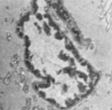
Example images and hand segmentations are shown in Figure 3 to highlight the difficulty of the cheek cell nuclei segmentation task. A variety of cells with unique nuclear morphologies were present. In addition, the fact that the sample may be sectioned at an arbitrary angle and position with respect to the nucleus may result in a series of varying shapes and contrast features depending on the section of the nucleus present.

Figure 3: Manual segmentation. TEM images of cheek cells (A,B) and the binary masks (C,D) constructed by hand tracing the outlines of the nuclei. Images of nuclei can often be quite contorted because of the angle at which they were sectioned. Image contrast of the nuclei with respect to the cytoplasm may vary because of the specimen preparation or the exposure conditions of the microscope. Hand segmentation is labor intensive and may be subjective among different operators.
Performance tests of the model
To understand whether the Deep ResUnet model was really learning to perform the nuclear segmentation task and not just remembering oddities or specifics of the training data, the accuracy of the model was assessed by comparing results from the model with held-out test data. The latter were additional images and hand segmentations that the model did not get to see or use during training. Although a relatively large number of hand-segmented images was used in this work, because they were part of a long-running project, most investigators who might use this deep learning algorithm would have considerably less data to work with.
The performance of the model was examined on the held-out test data while varying the amount of input training data. Figure 4 shows the impact of data augmentation on the effectiveness of the segmentation. Two experimental sets were trained with the same training set sizes, one with augmentation and one without. For both experimental sets, the performance drops off nonlinearly as the size of the training set is reduced. Since the model had no prior information about cells and nuclei, it learned exclusively by example. Overfitting can cause poor performance on unseen data. Clever regularization and optimization methods may not completely ameliorate this issue, so it is useful to determine a threshold for the number of training examples needed to achieve a quality prediction. Figure 4 shows that for two different performance assessments the threshold was about 150 training examples.

Figure 4: Performance of the Deep Residual U-Net model with and without data augmentation for automatic segmentation of human cheek cell nuclei. Data augmentation synthesizes “new” images from a small training set by introducing transformations (rotation, scaling, cropping) and noise to help the network learn information to aid predictions on unseen data. (A) Dice Loss test: pixels correctly determined divided by the total pixels, as a metric for segmentation quality versus the number of training examples. Data augmentation during training yields a better result regardless of the number of training examples. (B) Accuracy of auto-segmentation: model predictions compared with manual segmentation versus the number of training examples. The threshold for quality segmentation appears to be about 150 training examples.
The predicted segmentation for any arbitrary image can be obtained by passing a new image through the network and recording the output. Figure 5 shows that, again, 150 training examples appears to be the threshold for an acceptable automated segmentation.

Figure 5: After training with data augmentation and various numbers of training examples, two test images were passed through the network to get predictions. The model calculates the probability of a pixel being inside the nucleus. The image was then thresholded such that values higher than 0.6 were labeled “1”, while all other pixels were labeled “0”.. Effective segmentations can be produced for a variety of nuclei with different textures/shapes with 150 example training images.
Discussion
For all training set sizes in Figure 4, the model trained using data augmentation achieved a lower dice loss and a higher accuracy than the model trained without it. This suggests that augmentation is playing a significant role in forcing the model to learn generalizable information about the difference between cell cytoplasm and the nuclear envelope.
Figure 5 shows that even for the smallest number of training examples the deep network can either provide a crude localization of the nuclei or a skeletonized outline, assuming strong contrast for the nuclear membrane over the cytoplasm. The segmentation for the 150 training examples and above is strikingly similar to the hand segmented masks, demonstrating the power of deep learning for complex image processing tasks. The result from such fully trained networks requires no additional processing before use, allowing the model to operate as a “one-stop-shop” for end-to-end image processing. The data processing and machine learning strategy in this article may accelerate future work on more complicated image segmentation tasks, where even fewer training examples are available.
One complicating factor in this work is the heterogeneous nature of the cheek cell data-set, which is composed of many shapes of cells that present morphologically distinct nuclei, as seen in Figure 3. It is expected that for less complicated image processing tasks, the number of training images may be considerably fewer, since each image contains much more information regarding the population of example nuclei. In such cases where there exist several distinct “classes” of images within one dataset, it may be advantageous to split the data along such lines to simplify the training process.
Future work will examine the relative tradeoffs between training a single model on a large heterogeneous dataset versus several smaller homogenous classes. Overall, modern encoder-decoder architectures appear to be robust models for image processing tasks. Since the prediction takes place in milliseconds, these models make attractive solutions for handling the deluge of data currently emerging from modern microscopes. It is expected that as awareness of deep learning methods spread within the microscopy community, standards for recording and processing data will further leverage their scalability.
Conclusion
This article further establishes that automated segmentation of micrograph image features is feasible. Methods are shown for improving deep learning as an image processing framework for biological imaging. The use of image augmentation, in which a small number of hand-labeled images is transformed into a larger set through image transformations, allows strong performance even with the small numbers of images common to research environments. Such methods are not limited to TEM imaging; they should be equally applicable to X-ray microscopy and light microscopy. This work may inspire the application of deep learning methods in the imaging community in situations where conventional methods struggle.
Acknowledgments
The author would like to acknowledge the help of Karl Hujsak and Yue Li of Northwestern University for their mentorship and guidance with the preparation of this manuscript.


