


Introduction
Chemical inhomogeneity is key to the functioning of many systems, both biological and technical. For example, in organic photovoltaic cells, it is necessary to have domains of donor and acceptor close enough together, so carriers can diffuse between them (Li et al., Reference Li, Zhu and Yang2012). In battery research, the separation of nanoscale chemical phases is often indicative of the reaction kinetics or material degradation mechanisms (Boesenberg et al., Reference Boesenberg, Meirer, Liu, Shukla, Dell'anna, Tyliszczak, Chen, Andrews, Richardson and Kostecki2013). In both cases, the relevant length scale is often below 50 nm. One of the most important ways to understand such systems is to image them in a way which produces chemical, not just elemental contrast. In polymer systems, for instance, there is very little contrast of electron density, so non-spectral techniques produce little information. In battery electrodes, the important information may be the redox state of a transition metal cathode (Whittingham, Reference Whittingham2004). In all these systems, X-ray spectral microscopy has led to important advances. While there are a number of X-ray spectroscopic methods, scanning transmission X-ray microscopy (STXM) has proven to be a versatile method with a typical resolution of order 30 nm (Zhang et al., Reference Zhang, Balhorn, Mazrimas and Kirz1996; Collins & Ade, Reference Collins and Ade2012; Alqahtani et al., Reference Alqahtani, Babics, Gorenflot, Savikhin, Ferron, Balawi, Paulke, Kan, Pope and Clulow2018). A coherent-scattering based variant of this, ptychography, can improve the resolution to below 10 nm by using a phase retrieval process to reconstruct the probe and image separately (Schropp et al., Reference Schropp, Hoppe, Patommel, Samberg, Seiboth, Stephan, Wellenreuther, Falkenberg and Schroer2012; Shapiro et al., Reference Shapiro, Yu, Tyliszczak, Cabana, Celestre, Chao, Kaznatcheev, Kilcoyne, Maia and Marchesini2014; Holler et al., Reference Holler, Raabe, Diaz, Guizar-Sicairos, Wepf, Odstrcil, Shaik, Panneels, Menzel and Sarafimov2018; Deng et al., Reference Deng, Preissner, Klug, Mashrafi, Roehrig, Jiang, Yao, Wojcik, Wyman and Vine2019).
Like any experimental technique, STXM is prone to artifacts of several kinds. One of these, the subject of this paper, is that the spectral features of finely structured materials may be distorted due to the long tails of the point spread function (PSF) of the imaging element, typically a zone-plate lens. This distortion can come in two forms: a “hole effect” due to the probe beam sampling areas of widely differing optical density (OD) and the apparent mixing of spectra of species on either side of an interface. The former resembles the hole effect known from bulk X-ray spectroscopy (Goulon et al., Reference Goulon, Goulon-Ginet, Cortes and Dubois1982). To a certain extent, it is trivially obvious that a finite PSF will lead to spectral mixing at the interface between distinct chemical phases. However, the effect is exacerbated for diffraction-limited imaging systems where diffraction from the pupil casts light outside of the primary maxima of the PSF. The situation is worse still for partially obstructed pupils, typical of zone-plate-based X-ray microscopes, which have more intense sidelobes and can lead to spectral mixing over length scales several times the Rayleigh resolution of the optic.
Ptychographic microscopy, on the other hand, has been shown to achieve spatial resolution far superior to conventional scanning microscopy (Schropp et al., Reference Schropp, Hoppe, Patommel, Samberg, Seiboth, Stephan, Wellenreuther, Falkenberg and Schroer2012; Shapiro et al., Reference Shapiro, Yu, Tyliszczak, Cabana, Celestre, Chao, Kaznatcheev, Kilcoyne, Maia and Marchesini2014; Holler et al., Reference Holler, Raabe, Diaz, Guizar-Sicairos, Wepf, Odstrcil, Shaik, Panneels, Menzel and Sarafimov2018; Deng et al., Reference Deng, Preissner, Klug, Mashrafi, Roehrig, Jiang, Yao, Wojcik, Wyman and Vine2019). The imaging process uses a phase retrieval algorithm operating on coherent scattering data in a way that algebraically separates the probe and image. Thus, it can generate image data and associated spectral features free of artifacts relating to the PSF of the probe. That is not to say that ptychographic imaging provides a perfect record of the OD of the sample, but it does provide information on a scale finer than what STXM can, independent of the shape of the probe. In this article, we show through simulation on a model system how the PSF of a zone plate, in particular the long tails, leads to spectral distortions. Not only can the composition be misrepresented over surprisingly large distances from an interface, but, in extreme cases, the perceived composition profile can be qualitatively distorted. Furthermore, using experimental data from both conventional STXM and ptychographic microscopes, we show how STXM distorts known spectra from a real sample and that ptychography is able to recover the expected spectral profiles within the limits of the resolution of the technique. The effect of the PSF is further verified by a convolution of the ptychography data with the recovered probe which restores the spectral distortions.
In this paper, we first simulate a sharp interface between two chemically different materials, based on the calculated PSF of a zone plate, and demonstrate the spectral distortions resulting from STXM image formation. Then, we look at an actual sample in both STXM and ptychographic modes, using the same zone plate in the same microscope, and show the difference between the spectromicroscopic information gained from STXM and ptychography near the interface. Finally, we discuss the significance of the results and possible workarounds for the effects we see.
Materials and Methods
Calculation of Simulated STXM Spectra
We first simulated STXM spectra from a model system of trivial structure and known composition. Experimentally, STXM spectra are generated by measuring the same sample repeatedly across a range of energies. This provides an energy spectrum at each point in the material after the registration of the images. Those spectra will change from point to point according to the sample's chemical heterogeneity. Though poor image alignment can result in spectral distortions similar to what we discuss below, that step is not required for the simulation. The assumed sample consists of a semi-infinite region on the left (x < 0) consisting of one material and a semi-infinite region on the right made of another material of a different column density. Thus, the relevant characteristic of the focusing element is its knife-edge profile, which is the result of scanning the probe over the interface between a fully transparent region and one which is fully opaque. Thus, the knife-edge profile may be defined as follows:
 $$K( x) = \int_0^\infty {d{x}^{\prime}} \int_{-\infty }^\infty {dy{\rm PSF}( x-{x}^{\prime}, \;y) }, $$
where PSF(x,y) is the point spread function of the probe and the scan direction is taken as x. To calculate what this would be, we start with the two-dimensional Airy disk from a zone plate with a central stop, for which PSF is given by the following equation:
 $${\rm PSF}( r) {\kern 1pt} = {\kern 1pt} \left({\displaystyle{{2fa} \over {q( a^2-b^2) }}( {J_1( {raq}/f) -( b/a) J_1( {rbq}/f) } ) /r} \right)^2, $$
where q = 2π/λ, f is the focal length, a is the outer radius, J 1 is the J Bessel function of order 1, and b is the inner radius. The parameters used here are a = 125 μm, b = 45 μm, energy = 300 eV, and f = 1.5 mm, which are typical among conventional STXMs using a 25 nm outer zone width optics (Rayleigh resolution of 31 nm). To get the knife-edge profile, K(x) (x is the scan direction) we integrate (numerically) twice, once to get a line profile, i.e. the intensity pattern for an infinitely narrow vertical slot, and again to sum over positions of that slot for x ∈ [0,∞). Using the well-known asymptotic form of the J Bessel function, one can show that the PSF has an asymptotic r −3 +(oscillatory) form due to its sidelobes. The double integration that yields K(x) turns the distant sidelobes into an asymptotic x− 1 dependence, reflecting a long-range character.
In all that follows, we make the assumption made in the ptychographic theory (Guizar-Sicairos et al., Reference Guizar-Sicairos, Johnson, Diaz, Holler, Karvinen, Stadler, Dinapoli, Bunk and Menzel2014), which is that the electric field at any point  ${\vec{x}}^{\,\prime}$ on the downstream surface of the sample is the product of the probe field and the sample field transmission:
 $$\psi ( \vec{x}, \;{\vec{x}}^{\,\prime}) = O( \vec{x}\,) P( {\vec{x}}^{\,\prime}-\vec{x}\,), $$
where  $\vec{x}$ is the center position of the probe, $O( \vec{x}\,)$ is the field transmittance of the sample at point $\vec{x}$, and $P( \vec{y}\,)$ is the probe field at point $\vec{y}$. The transmitted intensity is the squared magnitude of the field:
 $$I( \vec{x}, \;{\vec{x}}^{\,\prime}) = T_{{\rm samp}}( {\vec{x}}^{\,\prime}) {\rm PSF}( {\vec{x}}^{\,\prime}-\vec{x}\,), $$
 by definition of the PSF and T samp = |O|2. The measured transmission,  $T( \vec{x}\,)$, is the integral over the sample surface of the local intensity:
 $$T( x) = \int {d^2{\vec{x}}^{\,\prime}T_{{\rm samp}}( {\vec{x}}^{\,\prime}) {\rm PSF}( {\vec{x}}^{\,\prime}-\vec{x}\,) } \;.$$
Now, the simulated sample we consider has a step-function transmission:
 $$T_{{\rm samp}}( \vec{x}\,) = \left\{{\matrix{ {T_1\;x < 0} \cr {T_2\;x \ge 0} \cr } } \right. = T_2\theta ( x) + T_1( 1-\theta ( x) ), $$
where θ(x) is the Heaviside step function and x is the component of  $\vec{x}$ along the scan direction, i.e. perpendicular to the interface. Given that the PSF has circular symmetry, we can express (5) as a double integral in x and y (the direction along the interface):
 $$T( x) {\kern 1pt} = \int_{-\infty }^\infty {d{x}^{\prime}T_{{\rm samp}}( {x}^{\prime}) } \int_{-\infty }^\infty {d{y}^{\prime}{\rm PSF}\left({\sqrt {{( x-{x}^{\prime}) }^2 + {{y}^{\prime}}^2} } \right)} , $$
where we can take y = 0 without loss of generality. Substituting (6) into (7) and defining the PSF as normalized to have an integral of 1, we have
 $$\eqalign{T( x) {\kern 1pt} & = {\kern 1pt} T_1\int_0^\infty {d{x}^{\prime}\int_{-\infty }^\infty {d{y}^{\prime}{\rm PSF}\left({\sqrt {{( x-{x}^{\prime}) }^2 + {{y}^{\prime}}^2} } \right)} } \cr &+ T_2\left({1-\int_0^\infty {d{x}^{\prime}\int_{-\infty }^\infty {d{y}^{\prime}{\rm PSF}\left({\sqrt {{( x-{x}^{\prime}) }^2 + {{y}^{\prime}}^2} } \right)} } } \right)\cr & = {\kern 1pt} K( x) T_1 + ( 1-K( x) ) T_2}, $$
where K(x) is the knife-edge profile of the probe.
Adding the energy dependence, the transmission through the sample, which is assumed to be of uniform thickness, is given by the following equation:
 $$\eqalign{T( x, \;E) & {\kern 1pt} = {\kern 1pt} K( x) T_1( E) + ( 1-K( x) ) T_2( E) \cr & = {\kern 1pt} K( x) \exp ( -{\rm O}{\rm D}_1S_1( E) ) \cr & \quad + ( 1-K( x) ) \exp ( {-}OD_2S_2( E) ) } , $$
where S 1, 2(E) are the assumed spectra of the materials on either side of the interface and OD1, 2 their effective thicknesses. These quantities S 1, 2(E) are proportional to the absorption coefficients (linear or mass) of the standard substances but normalized as convenient to be dimensionless. The idea is to remove dependence on details such as sample thickness. The extracted OD is the negative natural logarithm of this. Thus, the extracted spectrum at any point is,
 $$S( x, \;E) {\kern 1pt} = {\kern 1pt} -{\rm ln}( T( x, \;E) ) , $$
which is fitted to
 $$S_{{\rm fit}}{\kern 1pt} = {\kern 1pt} A_1( x) S_1( E) + A_2( x) S_2( E), $$
with the fit done for every x. Here, A 1, 2 are local estimates of the number of species 1,2 such that if there were no spectral blur or distortion, A 1,2 would be equal to OD1,2. They are derived by fitting the entire OD spectrum at each point to linear combinations of reference spectra, just as one would one when analyzing actual data. Note that in this analysis, the pre-edge absorption is considered to be just as much a part of the spectra of references and “sample” as the XANES part. When fitting the simulated pixel spectra, we fit the entire energy range including the pre-edge. This is the appropriate procedure for a system assumed to consist only of the two reference materials.
For our reference spectra, S 1, 2(E), we used C K-edge spectra of two polymers which have been used for organic photovoltaics, PC61BM and P3HT (Ulum et al., Reference Ulum, Holmes, Barr, Kilcoyne, Gong, Zhou, Belcher and Dastoor2013), scaled so that S 1, 2 = 1 at 320 eV, an energy beyond most of the chemistry-dependent features. These spectra are shown in Figure 1.

Fig. 1. Assumed reference spectra used in modeling of PC61BM (black) and P3HT (red), normalized to make intensities at 320 eV equal 1.
Experimental Comparison of Conventional and Ptychographic Spectromicroscopy
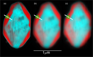
We demonstrate the spectral mixing effect experimentally by studying a two-phase material with known endmembers using both ptychography and conventional STXM. For this purpose, we chose a partially delithiated particle of LiFe2+PO4 similar to one which we have studied previously. When partially delithiated, micro-plates of LiFe2+PO4 have a core shell type structure with a sharp phase boundary at the interface (Boesenberg et al., Reference Boesenberg, Meirer, Liu, Shukla, Dell'anna, Tyliszczak, Chen, Andrews, Richardson and Kostecki2013; Yu et al., Reference Yu, Kim, Shapiro, Farmand, Qian, Tyliszczak, Kilcoyne, Celestre, Marchesini and Joseph2015). The outer, fully delithiated shell is Fe3+PO4 and has a roughly 100 nm width, while the core phase is more mixed with regions around morphological defects showing higher degrees of delithiation. This structure is ideal for our tests because it has a sharp interface between chemically distinct phases. However, the thickness is constant across the interface, so the large spectral distortion effect shown below for the simulated system with unequal thicknesses (Fig. 3) is not expected or seen.
The STXM and ptychography measurements were conducted at beamline 7.0.1.2 (COSMIC-Imaging) of the Advanced Light Source (Celestre et al., Reference Celestre, Nowrouzi, Padmore and Shapiro2018; Shapiro et al., Reference Shapiro, Celestre, Enders, Joseph, Krishnan, Marcus, Nowrouzi, Padmore, Park and Warwick2018) using a zone plate with inner and outer radii of 47.5 and 180 μm and 45 nm outer zones. To generate end-member reference spectra, we used Iterative Target Factor Analysis (Fernandez-Garcia et al., Reference Fernandez-Garcia, Marquez Alvarez and Haller1995) to find two apparent end-member spectra, then fit each pixel to linear combinations of these spectra, Then, we classified pixels by the loadings of each component in the fit and selected clusters of pixels having similar loadings within the cluster, but with the two clusters being as spectrally different from each other as possible. This procedure resulted in one cluster of pixels within the Fe3+PO4-rich shell and another occurring within the LiFe2+PO4-rich interior. The averaged spectra from these clusters were taken as the end-members for this test and are shown in a subsequent section. These spectra closely resemble ones previously derived from the Fe3+PO4–LiFe2+PO4 system14. For brevity, we refer to these end-members as FP and LFP, even though the compositions represented are somewhat mixed. Since the thickness of the particle was uniform, the normalization of the optical densities of the two end-member spectra is the same. A test for this supposition is that the sum of loadings for pixels in the Fe3+PO4- and LiFe2+PO4-rich areas should be equal, and they are, to within a few percent.
The STXM data were generated by two methods in order to confirm the effect of the PSF on the spectral content. First, conventional scanning microscopy data were generated in which total transmission is measured at each sample location by an integrating point detector. Second, for comparison, conventional image data were simulated by a convolution of high-resolution ptychographic reconstructions with the reconstructed probe. This will, in principle, generate STXM images with the same content as the conventional measurements but sampled on a high-resolution grid (5 nm pixels rather than 30 nm). For our tests of spectral distortion, we used the simulated STXM images because they are sampled on a finer grid than the actual STXM. The pixel spectra of the ptychography data were fit to sums of two end-member reference spectra, with nonnegative loading, plus a linear baseline. The results of this fit can be presented as a bicolor image, with red representing the loading of the FP end-member and cyan the LFP end-member. The STXM stack was derived by convolving each ptychographic image with the reconstructed probe function. The zone plate used had 45 nm outer zones and the probe had a diameter at a half-maximum value of 48 nm. The three versions (original ptychographic, simulated STXM, and real STXM) of the data are shown as bicolor images in Figure 4. In addition, non-ptychographic STXM was performed on the same sample, with the same zone plate in the same microscope as was used for the ptychographic stack (Fig. 4c).
Results
Simulated Interface
For the first calculation on the simulated polymer interface, we take OD1, 2 = 1, thus simulating a sample in which the C column density does not change across the interface but the composition does. The results are shown in Figure 2.

Fig. 2. Numerically fitted composition A 1, 2(x) across the model system of PC61BM/P3HT with equal effective thickness OD1, 2 = 1 at 320 eV (a) and simulated spectrum S fit (x = 0,E) with PSF estimation and fit at the interface x = 0 (b) in the case where the OD of each side is 1.0 at 320 eV. In (a), black and red curves are the fitted optical densities for PC61BM and P3HT; in (b), dots, solid black, and red are calculated data, fit, and residual.
The ideal forms for A 1, 2(x) would be step functions centered at x = 0. We see from Figure 2a that there is significant spectral mixing as far as 100 nm away from the interface, more than three times the outer zone width of the zone plate. Furthermore, the spectra near the interface are distorted, as can be seen from the fit and residual in Figure 2b. This distortion is an example of the hole effect. At the PC61BM peak energy (aromatic π ∗, 284.5 eV), the left half of the sample is nearly transparent, while the right half is highly absorbing. The transmission of the left half acts like stray light. A similar effect, with sides reversed, occurs at 287.5 eV, an energy at which P3HT is more absorbing than PC61BM. If the two ODs are not comparable, the distortion becomes especially severe and the errors in the OD of the thinner component become large, as shown in Figure 3, in which OD1 = 1 and OD2 = 0.01. There is a spurious peak in the fitted amount of the thin component as well as a broadening of the apparent profile of the thick component. The spectral fit at midpoint is particularly poor, yielding incorrect values for the ratio of OD between 287.5 and 284.5 eV as well as the peak heights.

Fig. 3. (a) Composition profile of PC61BM/P3HT model system in which the effective thicknesses of the two phases differ (OD1 = 1 and OD2 = 0.01). Dashed lines are the knife-edge profiles, weighted by the OD1,2, and solid lines the fits. The profiles for component 2 are multiplied by 5 to make them easier to see. (b) Simulated spectrum with PSF estimation and fit at the interface. In (a), black and red curves are the fitted composition for PC61BM and P3HT; in (b), dots, solid black, and red are calculated data, fit, and residual.
Experimental Results
Next, we shall show the experimental results on the mixed LFP–FP particle. Naturally, the STXM image shown in Figure 4c looks like a blurred version of the higher resolution ptychographic image (Fig. 4a). However, the FP-rich rim shows as a less saturated red color than in the original, suggesting that this area does not appear to be as spectrally pure as it does in the original stack. This visual impression is confirmed by lineouts of the loadings of the components, done along the line shown in Figure 4a. Figure 5 shows the derived profiles, and Figure 6 shows spectra taken at a point near an interface, linear-combination fits to those spectra and the spectral references used to construct Figures 5 and 6. We see that the STXM stack does indeed appear less phase pure over a range of 100 nm than the ptychographic stack. While these data are for an STXM stack simulated starting with a ptychographic stack, the profiles extracted from the actual STXM stack (Fig. 5, red points) are very similar to those from the simulated STXM, indicating that the mixing does indeed come from the PSF rather than some other source like image registration.

Fig. 4. Bicolor (red = FP-rich, cyan = LFP-rich) images of the test particle. The ptychographic image is shown on the left (a), the simulated STXM image in the middle (b), and the actual STXM image on the right (c). The white line shows the transect along which spectral profiles were taken. The green circle is centered around where the point spectra in Figure 6 were extracted.

Fig. 5. Fit results for point spectra along the transect shown in Figure 4. The black lines show the sum of the loadings for FP and LFP  $( { A}_{{\rm LFP}}{\rm} + {A}_{{\rm FP}})$ and the red lines the fraction of FP (A FP/(A LFP + A FP)). The solid lines refer to the ptychographic data (Fig. 4a) and the dashed lines to the simulated STXM (Fig. 4b). The red points refer to the actual STXM data. The match with the simulated STXM is imperfect because the actual STXM data were taken with the sample in a different orientation from the ptychographic data, and with a coarser grid of pixels. The blue vertical line shows the location for the point spectra, as shown in Figure 6.

Fig. 6. Reference spectra (top and bottom curves, black) and point spectra (red) on the ptychographic (upper) and simulated-STXM (lower) stacks, at the point corresponding to the blue line in Figure 5. The solid lines are the data and the dashed are the fits to a linear combination of the references.
Discussion and Conclusions
We demonstrate from the simulations shown in Figures 2 and 3 that conventional STXM can result in significant (>10%) spectral mixture effects at distances from the midpoint between two distinct chemical phases out to about 100 nm, or more than three times the outer zone width. When the optical densities on either side of the interface are very different (Fig. 3), the effects can persist out to 300 nm from the interface. For an optically thick sample, the data may not fit well to a linear combination of the reference spectra, even if these spectra accurately represent the makeup of the sample, as illustrated in Figure 3. We also see that if there is a thickness step, the spectra can be distorted near the step due to hole effect. One might imagine that apodizing the zone plate would remove the long tails on the PSF. To test this idea, we simulated a zone plate apodized at inner, outer, or both edges (see Supplementary material) as well as a hypothetical, perfect Gaussian probe. We find that the artifacts we have been discussing are modestly (factor of 2 or 3) reduced by apodizing the outer edge of the zone plate, but not by nearly as much as a perfect Gaussian probe would do. In particular, spectral distortions of >100 nm away from the interface of the polymer model are nearly eliminated by the Gaussian probe but not by the apodized zone plate.
Another approach is to use an off-axis zone plate as proposed by Takayama et al. (Reference Takayama, Fukuda, Kawashima, Aoi, Shigematsu, Akada, Ikeda and Kagoshima2021). This method, in which a beam-defining aperture is used to illuminate a part of the zone plate that does not include the center, produces a probe with sharp edges. However, the resulting beam is deflected from the incident beam by an energy-dependent angle, so the sample would have to move in two axes as a function of energy. Also, the zone plate has to be larger and contains more and finer zones than one that produces a similar probe size on-axis. These issues present difficult but not impossible engineering challenges.
Given that the ptychographic data have superior resolution to STXM, it may seem reasonable to perform only ptychographic measurements. However, microscopy at higher resolution than STXM requires much longer exposure times than STXM for the same beam conditions. STXM data are simpler to acquire and process than ptychograpic data and they can provide an excellent qualitative analysis of nano-materials and a quantitative analysis of larger structures. The results presented here both argue strongly for the use of ptychography when feasible and careful interpretation of STXM data when the chemical phases approach the spatial resolution of the microscope. Interpretation can be greatly aided by the use of correlative measurements with other probes such as electrons.
While the above modeling and experiment deal only with a zone plate as the imaging element, the qualitative nature of the results should also apply to other focusing elements whose PSFs have long tails. These would include any element in which the spatial resolution is limited by diffraction through an effective pupil-plane aperture with sharp edges.
Availability of data and materials
The data that support the findings of this study are available from the corresponding author upon reasonable request.
Supplementary material
To view supplementary material for this article, please visit https://doi.org/10.1017/S1431927621012733.
Acknowledgments
We thank N. Holmes and M. Barr for the use of the polymer reference spectra.
Author contributions statement
M.A.M. performed the data analysis and modeling. D.A.S. and Y.-S.Y. acquired the data and performed the ptychographic reconstructions.
Financial support
The operations of the Advanced Light Source are supported by the Director, Office of Science, Office of Basic Energy Sciences, US Department of Energy under Contract No. DE-AC02-05CH11231.


 Open access