


Introduction
The development of ultrafast cameras for transmission electron microscopy (TEM) such as the pnCCD (Müller et al., Reference Müller, Ryll, Ordavo, Ihle, Strüder, Volz, Zweck, Soltau and Rosenauer2012; Ryll et al., Reference Ryll, Simson, Hartmann, Holl, Huth, Ihle, Kondo, Kotula, Liebel, Müller-Caspary, Rosenauer, Sagawa, Schmidt, Soltau and Strüder2016), the Medipix3 chip (Plackett et al., Reference Plackett, Horswell, Gimenez, Marchal, Omar and Tartoni2013), delay-line detectors (Oelsner et al., Reference Oelsner, Schmidt, Schicketanz, Klais, Schönhense, Mergel, Jagutzki and Schmidt-Böcking2001; Müller-Caspary et al., Reference Müller-Caspary, Oelsner and Potapov2015), or the EMPAD (Tate et al., Reference Tate, Purohit, Chamberlain, Nguyen, Hovden, Chang, Deb, Turgut, Heron, Schlom, Ralph, Fuchs, Shanks, Philipp, Muller and Gruner2016) enabled the collection of the full diffraction space up to a flexible cutoff spatial frequency at each scan point in scanning TEM (STEM). This technology paved the way for momentum-resolved STEM techniques with high samplings in both real and diffraction space, sometimes being referred to as 4D-STEM. Acquisitions with a detector frame rate of several kHz are currently achieved by employing these cameras. In particular, the mapping of electric fields and charge densities down to the atomic scale (Müller et al., Reference Müller, Krause, Beche, Schowalter, Galioit, Löffler, Verbeeck, Zweck, Schattschneider and Rosenauer2014), meso-scale strain, and electric field measurements by nano-beam electron diffraction (Müller-Caspary et al., Reference Müller-Caspary, Oelsner and Potapov2015), and, furthermore, electron ptychography (Hoppe, Reference Hoppe1969; Hegerl & Hoppe, Reference Hegerl and Hoppe1970) have been enabled by this dramatic detector speed enhancement (Rodenburg & Bates, Reference Rodenburg and Bates1992; Rodenburg et al., Reference Rodenburg, McCallum and Nellist1993; Nellist et al., Reference Nellist, McCallum and Rodenburg1995; Humphry et al., Reference Humphry, Kraus, Hurst, Maiden and Rodenburg2012; Jiang et al., Reference Jiang, Chen, Han, Deb, Gao, Xie, Purohit, Tate, Park, Gruner, Elser and Muller2018).
Due to its excellent dose efficiency (Zhou et al., Reference Zhou, Song, Kim, Pei, Huang, Boyce, Mendonça, Clare, Siebert, Allen, Liberti, Stuart, Pan, Nellist, Zhang, Kirkland and Wang2020), STEM ptychography as a method to retrieve the complex object transmission function has gained increasing interest. Four-dimensional (4D) data sets combining real and diffraction space information have been shown to provide enormous flexibility in post-acquisition processing. For example, ptychography has been demonstrated to be capable of both resolution improvement and aberration correction after the acquisition using computational methods (Nellist et al., Reference Nellist, McCallum and Rodenburg1995; Gao et al., Reference Gao, Wang, Zhang, Martinez, Nellist, Pan and Kirkland2017). It achieves a better signal-to-noise ratio for weak phase objects than annular bright field or differential phase contrast (Seki et al., Reference Seki, Ikuhara and Shibata2018) and allows reconstruction at extremely low dose (O'Leary et al., Reference O'Leary, Allen, Huang, Kim, Liberti, Nellist and Kirkland2020).
The high data rates require an efficient implementation of advanced methods for imaging contrast via post-processing in order to minimize the duration of numerical processing. Ultimately, computing and software implementation capabilities are desirable that allow for the live reconstruction of the ptychographic phase and amplitude, first moments, electric fields, and charge densities, for example.
During experiments, a region of interest is usually selected via imaging employing conventional STEM detectors. Weakly scattering and beam-sensitive specimens, where ptychography and first moment imaging (Waddell & Chapman, Reference Waddell and Chapman1979; Müller et al., Reference Müller, Krause, Beche, Schowalter, Galioit, Löffler, Verbeeck, Zweck, Schattschneider and Rosenauer2014) can be most advantageous, generate poor contrast in conventional imaging modes and quickly degrade using typical beam currents in conventional STEM (Peet et al., Reference Peet, Henderson and Russo2019). 4D-STEM analyses are normally applied after data acquisition and transfer to a data processing workstation. It is, therefore, not possible to be certain that the selected region and microscope settings were appropriate until after successful reconstruction. For that reason, one often acquires a larger number of data sets, which takes considerable storage space in the case of 4D-STEM. In contrast, a fast implementation of the considered computational methods would allow performing this data evaluation live during the experiment.
In this study, we demonstrate 4D-STEM continuous live scanning with the simultaneous ptychographic single-sideband (SSB) reconstruction combined with bright field, annular dark field, and first moment imaging, including its divergence which is proportional to the charge density in thin specimens. To this end, the ptychographic algorithm was first reformulated mathematically. This allows navigation on the sample and change of microscope parameters with a live view of the reconstruction, alongside signals from other 4D-STEM techniques. Second, we use SrTiO3 and In2Se3 to demonstrate the live evaluation capability of our approach in experiments by in situ processing of the data stream of an ultrafast camera. Third, the results obtained live are validated by conventional post-processing. Particular attention is drawn to the capability of SSB to provide reliable structural images, to reconstruction artifacts arising from processing partial scans and to reconstructing nonperiodic objects. Moreover, the performances of SSB ptychography and the enhanced ptychographic engine (ePIE) are compared, interestingly pointing toward SSB being significantly more robust against dynamical scattering in terms of qualitative structural imaging. This article closes with a detailed discussion and a summary.
Materials and Methods
Live Imaging
A continuous live scanning display for large-scale 4D-STEM data benefits greatly from a data processing method where smaller portions of input data are processed independently and merged progressively into the complete result. For virtual detectors and first moments, often referred to as “center-of-mass (COM)”, this is trivial to achieve since each detector frame, that is, diffraction pattern, produces an independent entry in the final data set which allows frames to be processed individually, accumulating results in a buffer. Displaying the contents of this buffer at regular intervals provides a live-updating view.
In contrast, ptychography generates results by putting detector frames from the entire data set, or at least a local environment, in relation to each other. Consequently, adapting the methodology so as to circumvent the processing of the entire data set at once, thus gradually merging partial results extracted from portions of the input data into the complete result, is necessary. As previously demonstrated by Rodenburg & Bates (Reference Rodenburg and Bates1992), Rodenburg et al. (Reference Rodenburg, McCallum and Nellist1993), and Pennycook et al. (Reference Pennycook, Lupini, Yang, Murfitt, Jones and Nellist2015), both phase and amplitude information can be extracted from a set of diffraction patterns (usually restricting to the Ronchigram region) by performing the Fourier transform of the 4D data set with respect to the scan raster and reordering the dimensions. Depending on the model presumed for the interaction between specimen and incident STEM probe, the direct inversion of the data can either be done by Wigner Distribution Deconvolution (WDD) or the SSB ptychography scheme (Rodenburg et al., Reference Rodenburg, McCallum and Nellist1993). Whereas WDD is based on a single interaction with an arbitrary complex object transmission function and is capable of separating specimen and probe, the weak phase approximation
 $$\psi_{{\rm exit}}( \vec{r}) = \psi_{{\rm probe}}( \vec{r}) \cdot{\rm e}^{{\rm i}\Phi}\approx \psi_{{\rm probe}}( \vec{r}) \cdot( 1 + {\rm i}\phi( \vec{r}) ) $$
governs the SSB approach. Here, the specimen exit wave at a given scan point can be expressed by a multiplication of the probe wave function  $\psi _{{\rm probe}}( \vec {r})$ with the first-order Taylor expansion of a phase object with phase distribution $\Phi ( \vec {r})$. It is, hence, limited to weakly scattering ultrathin objects, for example, thin light matter investigated with relativistic electrons. Any quantitative interpretation of SSB reconstructions of real data should, therefore, be examined critically since equation (1) breaks down quickly with increasing thickness. Its capability of direct, dose-efficient phase recovery makes it nevertheless attractive for the in situ qualitative assessment of specimen and imaging conditions. A more advanced ptychography scheme can still be applied after recording. Because a data point in the final reconstruction depends on all recorded scan points, the reconstruction is only accurate if it is applied to the full 4D data.
We refer to original work for a derivation of the conventional SSB methodology (Rodenburg & Bates, Reference Rodenburg and Bates1992; Pennycook et al., Reference Pennycook, Lupini, Yang, Murfitt, Jones and Nellist2015) and give a concise summary here. The first processing step consists of Fourier transforming the 4D data cube as to the scan coordinate, translating the scan coordinate in real space to spatial frequencies  $\vec {Q}$ sampled by the scanning probe. This new 4D data cube can be ordered such that each scan spatial frequency defines one plane. By employing the weak phase object approximation in equation (1), Rodenburg et al. have shown analytically that the data in each plane is described by three discs of the size of the probe-forming aperture, positioned at the origin and as Friedel pairs at the positions defined by the spatial frequency vector $\vec {Q}$. Importantly, double overlaps as depicted schematically in Figure 1 contain the complex Fourier coefficients of iΦ, potentially affected by aberrations of the probe-forming system. The double overlap regions are often referred to as trotters colloquially.
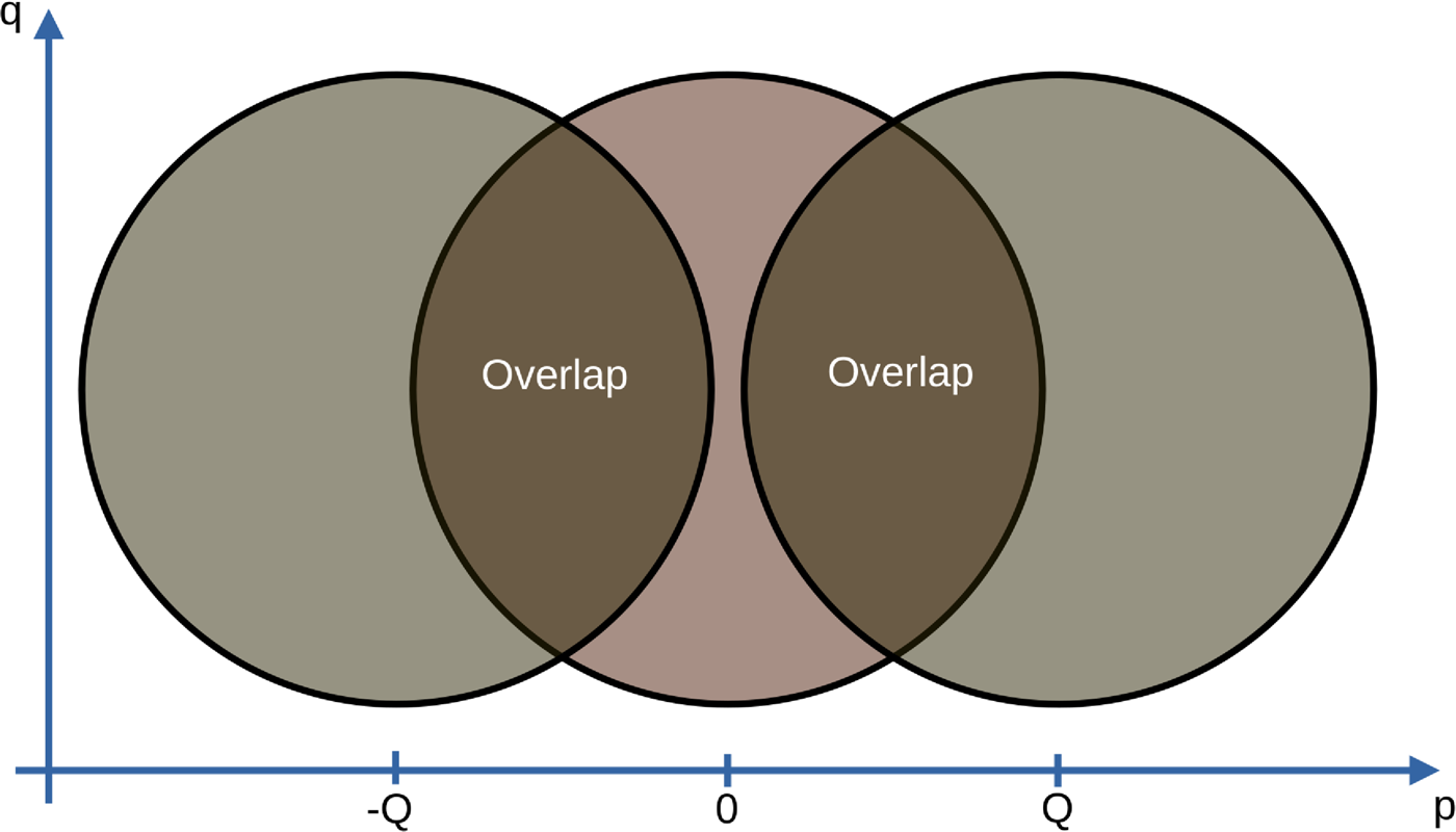
Fig. 1. Double overlap regions in the planes of the Fourier transformed 4D data cube are defined by three circles of the size of the probe-forming aperture. The distance Q between the circles is determined by the currently considered spatial frequency of the scan raster and defines the spatial frequency of Φ reconstructed in this plane of the data cube. Potential triple overlaps for small Q need to be excluded.
The ptychographic SSB reconstruction is a linear function of the input data since the result is obtained with a sequence of linear transformations, such as Fourier transforms, element-wise multiplication, and summation (Pennycook et al., Reference Pennycook, Lupini, Yang, Murfitt, Jones and Nellist2015). Such linear functions are particularly suitable for incremental processing since they are additive. Mathematically, the complete input data can be understood as the sum of smaller individual data portions that are padded with zeros to fill the shape of the complete data set. Additive functions allow to calculate the complete result by accumulating the processing results of zero-padded portions in any subdivision and order. Furthermore, intermediate results can be extracted at any desired stage from the yet incomplete sum of results.
However, directly processing zero-padded data this way is very inefficient for computationally demanding algorithms such as ptychography employing large 4D-STEM data, because the processing effort and memory consumption is amplified by the number of subdivisions. For that reason, the algorithm should be reformulated to process smaller input data portions without zero-padding. The additivity and homogeneity of linear functions gives ample freedom to restructure the underlying data processing flow toward this goal, allowing development of mathematically equivalent implementations that are optimized for live imaging.
In the particular case of SSB ptychography, individual spatial frequencies of the result  $\Phi ( \vec {r})$ are extracted from spatial frequencies of signals at specific scattering angle ranges within the double overlaps (Rodenburg et al., Reference Rodenburg, McCallum and Nellist1993; Pennycook et al., Reference Pennycook, Lupini, Yang, Murfitt, Jones and Nellist2015) introduced in Figure 1.
Suppose we have the intensity of diffraction patterns present as 4D data, which is written as  ${\bf D}_{xy} \in {\opf R}^{m \times n} \ {\rm where} \ x \in [ s_x] ,\; y \in [ s_y]$ and the notation [s x] represents the set of natural numbers not exceeding s x − 1. That is, [s x] : = {0, 1, …, s x − 1} with the total number of elements s x. The indices x, y represent the scan position index, with the total number of scanning steps being s x and s y in each direction. Each matrix D is a diffraction pattern (d pq) where p and q represent the pixel index on the detector with dimension m × n. Each pixel index p q corresponds to a scattering angle, or equivalently, spatial frequency in the specimen.
We can write the Fourier transform with respect to the scan raster as
 $$( f_{\,pq}) _{kl} = \sum_{x = 0}^{s_x-1} \sum_{y = 0}^{s_y-1} ( d_{\,pq}) _{xy} \, {\rm e}^{-{\rm i}2\pi( {xk}/{s_x} + {yl}/{s_y} ) },\; $$
where k and l denote the spatial frequencies in the scan dimension, taking the places of x and y. Therefore, we obtain a 4D data set in the spatial frequency domain, that is,  ${\bf F}_{kl} \in {\opf C}^{m\times n}$.
The next step in SSB is to apply a filter  ${\bf B}_{kl} \in {\opf C}^{m \times n}$ for each tuple of spatial frequencies kl that calculates the weighted average of the spatial frequency signal over specific ranges of pixels, that is scattering angles pq, that can have positive or negative weight as defined by the trotters. It should be noted that the structure of this filter is different for each tuple of spatial frequencies.
Using (2), we can write the reconstruction in the Fourier domain p kl as
 $$\eqalign{\,p_{kl} & = \sum_{\,p = 0}^{m-1} \sum_{q = 0}^{n-1} ( f_{\,pq}) _{kl} ( b_{\,pq}) _{kl}\cr & = \sum_{\,p = 0}^{m-1} \sum_{q = 0}^{n-1} \left[\sum_{x = 0}^{s_x-1} \sum_{y = 0}^{s_y-1} ( d_{\,pq} ) _{xy} \, {\rm e}^{-{\rm i}2\pi( {xl}/{s_x} + {yk}/{s_y}) }\right]( b_{\,pq}) _{kl}\cr & = \sum_{x = 0}^{s_x-1} \sum_{y = 0}^{s_y-1} \left[\sum_{\,p = 0}^{m-1} \sum_{q = 0}^{n-1}( b_{\,pq}) _{kl}( d_{\,pq}) _{xy} \right]{\rm e}^{-{\rm i}2\pi( {xk}/{s_x} + {yl}/{s_y}) }.}$$
The reformulation is given by interchanging the summation and the index dimension of detector and the index of scan points in the real and frequency domain, respectively. This nested summation can be pruned without changing the result by skipping parts that are known to yield zero, for example calculations for empty double overlap regions. Note that p kl essentially represents the Fourier coefficients of iΦxy in equation (1) which are potentially affected by aberrations of the probe-forming system.
The inner part of equation (3) can be implemented with a matrix product between B and D. The outer sum over x and y can then be subdivided and reordered to process the input data D incrementally in smaller portions. Numerically, the filter matrix Bkl can be stored efficiently as a sparse matrix since the trotters for the highest frequencies are often empty (no overlap), and, for many frequencies, the double overlap region where the filter is nonzero, is small.
As an intermediate summary, this formulation translates the SSB scheme to a matrix product of a partial input data matrix with a sparse matrix containing the double overlap regions. Elements of a Fourier transform are then applied to the result of this matrix product. This generates a partial reconstruction result in the frequency domain that covers the entire field of view. The partial reconstructions for all partial input data portions are accumulated in a global buffer using a sum, as described above. For a live view of the reconstruction in the spatial domain, the contents of this buffer can be inversely Fourier transformed at any desired time to show the transmission function of the specimen within the weak phase object approximation.
We used LiberTEM (Clausen et al., Reference Clausen, Weber, Ruzaeva, Migunov, Baburajan, Bahuleyan, Caron, Chandra, Dey, Halder, Katz, Levin, Nord, Ophus, Peter, Schyndel van, Shin, Sunku, Müller-Caspary and Dunin-Borkowski2020a) as a data processing framework since it is optimized for MapReduce-like approaches and designed with live data processing capabilities in mind (Clausen et al., Reference Clausen, Weber, Ruzaeva, Migunov, Baburajan, Bahuleyan, Caron, Chandra, Halder, Nord, Müller-Caspary and Dunin-Borkowski2020b). LiberTEM user-defined functions (UDFs) provide the application programming interface (API) to efficiently implement operations that follow the described pattern: A method to process a stack of frames that is called repeatedly, task data to store constant data such as the sparse matrix for the double overlaps, result buffers of arbitrary type and shape, and user-defined merging operations to generate a result of arbitrary complexity from partial results. Furthermore, LiberTEM allows to update a result display each time a partial result is merged. UDFs for first moment analysis and virtual detectors were already implemented before for offline data analysis.
To run the UDFs on live data, we implemented a prototype live UDF back-end that allows to run a set of UDFs on data from a Quantum Detectors Merlin for EM Medipix3 for electron microscopy (Plackett et al., Reference Plackett, Horswell, Gimenez, Marchal, Omar and Tartoni2013; Quantum Detectors, 2019). It uses multiple CPU cores for decoding the raw data from the detector, and a single GPU for the main processing task, which was sufficient for this application. A production-ready version with support for multiple processing nodes, further enhanced use of multiple CPUs and multiple GPUs similar to the offline data processing capabilities of LiberTEM is being designed at the time of writing and will be published as open-source as a part of LiberTEM.
For comparison, ePIE (Maiden & Rodenburg, Reference Maiden and Rodenburg2009) based ptychographic reconstructions have been performed in post-processing as it can reconstruct both the complex object transmission function and the complex illumination, still presuming single interaction of probe and specimen, but considering an arbitrary complex object transmission function. This was done to check whether the straightforward SSB approach compromises the quality of the result compared with more advanced ptychographic schemes. It has to be noted that, as an iterative method, ePIE is not suitable for live imaging in the current realizations.
Material System
We demonstrate live processing using two different specimens. First, indium selenide (In2Se3) was used to highlight the advantages of live ptychography and center of mass in comparison to conventional STEM (Ye et al., Reference Ye, Soeda, Nakamura and Nittono1998). Second, a strontium titanate (SrTiO3) lamella with the electron beam incident along the [100] axis for a more quantitative analysis was used. The latter is stable and provides good contrast in conventional STEM for comparison and adjustments, is well-characterized, and at the same time can highlight the ability to also resolve the light oxygen columns that are difficult to image with reliable contrast by conventional STEM techniques (Browning et al., Reference Browning, Pennycook, Chisholm, McGIBBON and McGIBBON1995). Too small double overlap regions with an area of less than 10 px were omitted in live processing to avoid the introduction of excessive noise. This can be understood as a band-pass filter applied to exclude the high frequencies close to the transfer limit of SSB ptychography which corresponds to twice the radius of the probe-forming aperture.
Experimental Setup
First moment imaging and ptychography require the correct alignment and calibration of the scan (specimen) coordinate system with respect to the detector coordinate system. The convergence angle of the incident probe was measured with a polycrystalline gold specimen. Employing parallel illumination first, the (111) gold diffraction ring was used to calibrate the diffraction space assuming a lattice constant of gold of 0.4083 nm (Villars & Cenzual, Reference Villars and Cenzual2016). With the known wavelength, the convergence semi-angle was determined to 22.1 mrad from a Ronchigram recorded in the same STEM setting as used in the actual experiment.
The rotation of the detector coordinate system with respect to the scan axes was determined by minimizing the curl of the first moment vector field and making sure that the divergence of the field is negative at atom positions. Note that, in theory, the curl of purely electrostatic fields should vanish. The pixel size in the scan dimension was taken from the STEM control software during live processing and verified by comparison with the known lattice constant of SrTiO3. The residual scan distortion, that is, the translation of the diffraction pattern as a whole during scanning, was not compensated for since it turned out to be negligible at the atomic-resolution STEM magnifications used in this analysis.
Data were acquired at a probe-corrected FEI Titan 80-300 STEM (Heggen et al., Reference Heggen, Luysberg and Tillmann2016) operated at 300 kV. The microscope was equipped with a Medipix Merlin for EM detector operated at an acquisition rate for a single diffraction pattern of 1 kHz in continuous mode. The scan size was 128 × 128 scan points and the recorded diffraction patterns had a dimension of 256 × 256 pixel. In addition, the high-angle annular dark-field (HAADF) signal has been recorded with a Fischione Model 3000 detector covering an angular range of 121.7 mrad to approximately 200 mrad. The upper limit is defined by apertures of the microscope rather than by the outer radius of the detector. The run time for each step of the data processing flow was measured using the line-profiler Python package.
Results
Live Processing
The performance of our approach is demonstrated in Figure 2 which depicts (a) the structure of In2Se3 together with the projected potential and (b) snapshots of the reconstructed phase in nanosheets of this material using SSB ptychography at different stages of the scan. The reconstruction is performed progressively such that only the diffraction patterns of incoming scan pixels are processed and added to the final reconstruction according to equation (3) in which all pixels are affected. Whereas current research in the field of materials science explores ultrathin In2Se3 as a candidate for 2D ferroelectrics, this specimen was chosen due to its robustness against electron dose for the methodological development. The data in Figure 2b were taken from a live video recorded during the STEM session, being available as the Supplementary material.
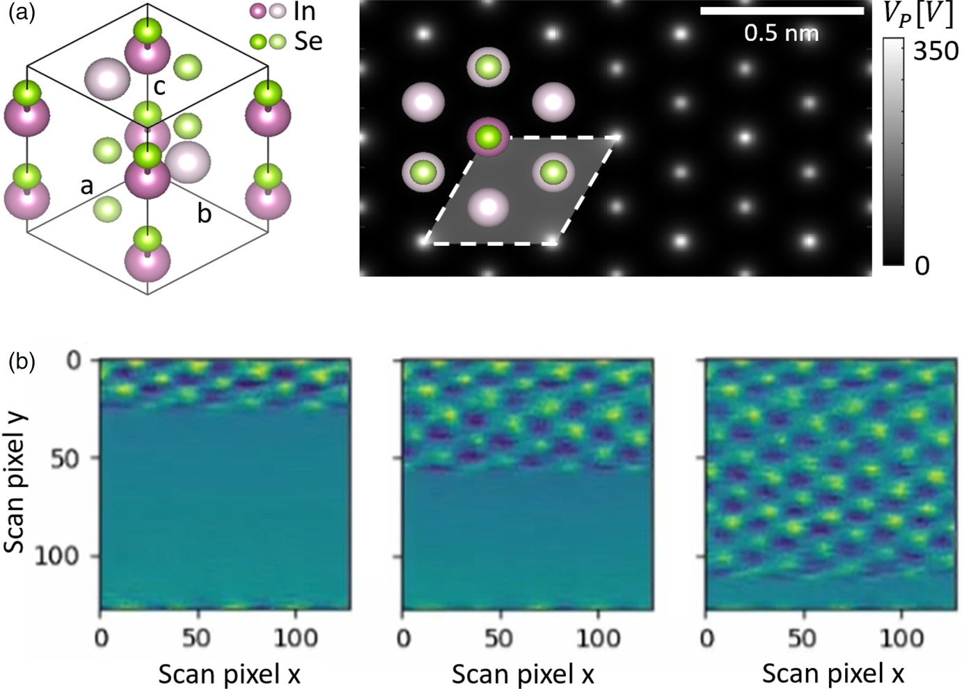
Fig. 2. Investigation of In2Se3 nanosheets. (a) 3D view of the unit cell (left) and electrostatic potential projected along  $\vec {c}$(right). Note the different densities of atoms in c-direction at different sites. (b) Snapshots of live ptychography (phase) using the SSB scheme at different stages of the scan.
In general, the quality of the ptychographic reconstruction strongly depends on matching the position and radius of the (usually circular) aperture function on the detector with the double overlap regions. Even small deviations lead to a mismatch between the mask borders and the edges of the zero-order disk, which adds noise and reconstruction errors from those erroneous border pixels. A precise alignment can be done, for example using a position-averaged diffraction pattern or by recording the bright-field disc with the specimen removed from the field of view, as in our analyses.
It must be pointed out that a partial SSB reconstruction only approximates the result because not all spatial frequencies have been completely sampled at this point. However, it is already possible to see the atom columns in the partial reconstructions. This allows time- and dose-efficient live focusing and navigation to regions of interest on specimens. In Figure 3, complete reconstructions of In2Se3 are shown. All atom columns can be seen clearly in the bright-field images, in the divergence of the first moment and in the phase of the object transmission function obtained by SSB ptychography. All signals were calculated live from the 4D-STEM data stream.

Fig. 3. Live imaging of In2Se3 nanosheets at atomic resolution for a 128 × 128 STEM scan. The atom columns are visible in all methods. The semi-convergence angle was 22.1 mrad.
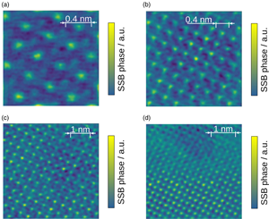
Figure 4 depicts the phase of ptychographic SSB reconstructions of SrTiO3 performed live while changing microscope parameters such as the STEM magnification (scan pixel size) in Figures 4a–4c, and the probe focus in Figure 4d. The full video showing live updating during continuous scanning while microscope parameters are changed is available in the Supplementary material.
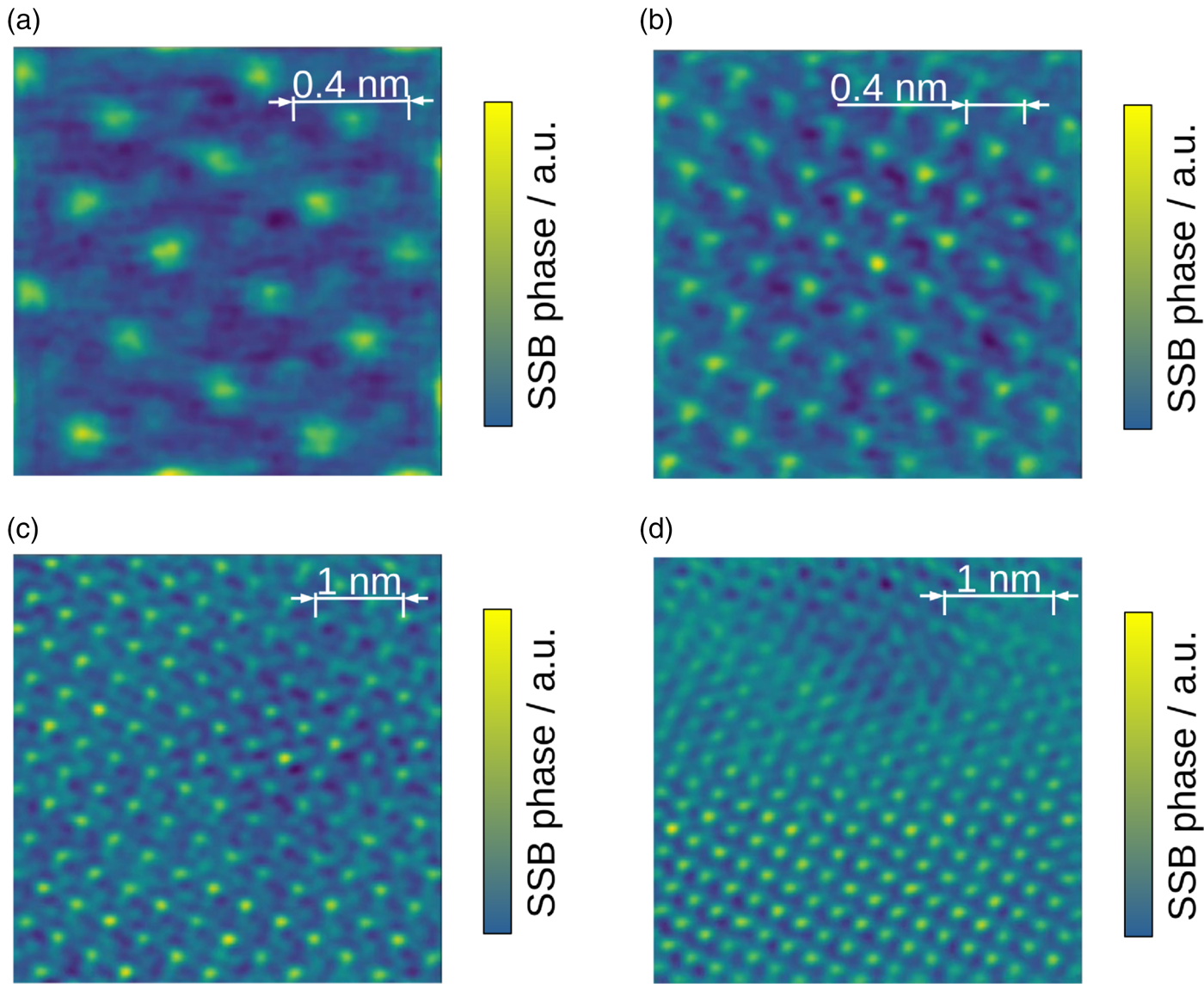
Fig. 4. Live variation of microscope parameters on SrTiO3: During live reconstruction the parameters for SSB were not changed. From (a) to (c), the magnification is reduced. If the magnification is reduced further, SSB fails. In (d), the focus is changed during acquisition. The semi-convergence angle was 22.1 mrad.
Although the inherent reconstruction parameters are naturally robust against a change of the probe focus for direct ptychography schemes that do not intend to correct aberrations, a magnification change influences the relation between a spatial frequency in the reconstruction in pixel coordinates, and the pixel distance in sample coordinates. This means that the geometry of a double overlap region that contains the signal to reconstruct a certain spatial frequency in the result changes with magnification. In the strict sense, changing the magnification without updating the scan step size (and double overlap masks) in the reconstruction is, therefore, mathematically inaccurate. In practice, however, it is desirable to be able to lower the magnification so as to navigate coarsely to a specimen region of interest without a new calibration or pre-calculation of the masks Bkl in equation (3) to be time-efficient, and then observe or record details after switching back to the correct magnification again. Therefore, we studied to which extent the reconstruction is robust against a magnification change despite keeping the internal SSB parameters unchanged in Figures 4a–4c. It showcases that the structural contrast is in general maintained. A possible future development with only a moderate effort could be pre-defining double overlap masks for common magnifications in order to build a look-up table that solves inaccuracies. We assume without loss of generality regarding the algorithmic structure, that live processing is required at a dedicated magnification being equal to the final recording where data are actually stored, and mention a certain robustness against changes of the scan pixel size as a valuable side note.
Computational Details
In our implementation, the sparse matrix product was the throughput-limiting step. By using an efficient GPU implementation from cupyx.scipy.sparse (CuPy), this could be accelerated sufficiently to allow processing of over 1,000 frames per second at suitable parameters, enabling for live imaging using a Medipix3 sensor.
The memory consumption of the current SSB ptychography implementation scales as  ${\cal O}( N)$ with the number of scan points at a constant aspect ratio since the number of spatial frequencies to reconstruct scales linearly with the number of scan points, and each reconstructed frequency adds a double overlap region. These regions sample the diffraction data more densely when extracting more spatial frequencies, meaning that the average number of nonzero entries per trotter is roughly constant for a given pixel size and beam parameters. As the processing time for dense-sparse matrix products roughly scales linearly with the number of nonzero entries in the sparse matrix and the number of vectors in the dense matrix, SSB scales poorly with ${\cal O}( N^{2})$ in computation time with the number of scan points.
The size of the matrix containing the double overlap regions is highly dependent upon the acquisition parameters in the present implementation. A larger camera length increases the Ronchigram size, consequently increasing nonzero entries. The relationship between scan pixel size and the convergence angle changes the spatial frequency limit above which no double overlaps occur. The less often spatial frequencies create double overlaps, the smaller the matrix B becomes. In this study, the scan area for live processing was limited to a size of 128 × 128 and microscope parameters were chosen to keep the matrix size low enough to fit into the GPU RAM.
Post-Processing
We concentrated up to this point, solely on the live evaluation in order to facilitate optimization of experimental parameters during the session. This avoided the need for saving vast amounts of 4D-STEM data that would have required significant disc space due to the continuous nature of the experiments. During the experiments, only a few reliable data sets were recorded. To verify the reliability of our approach, we compared the post-processing of the recorded data against the live experiment to determine if the inherent parameters used in post-processing, such as the Ronchigram position and radius, are in sufficient agreement with those of the live results.
In Figure 5, the post-processing of In2Se3 data is shown. Here, the two different atom columns highlighted in Figure 2a can be seen in the first moment vector field (Fig. 5a), in its divergence (Fig. 5b), and in the HAADF image (Fig. 5c). The phase of the SSB reconstruction (Fig. 5d) also yields site-specific contrast, which is more pronounced than in the live imaging result in Figure 3d. Recalling that SSB ptychography relies on the weak phase object approximation in equation (1) that breaks down already at the thinnest of specimen as to a quantitative interpretability, conclusions from relative phases among different atomic sites need to be drawn with great care.
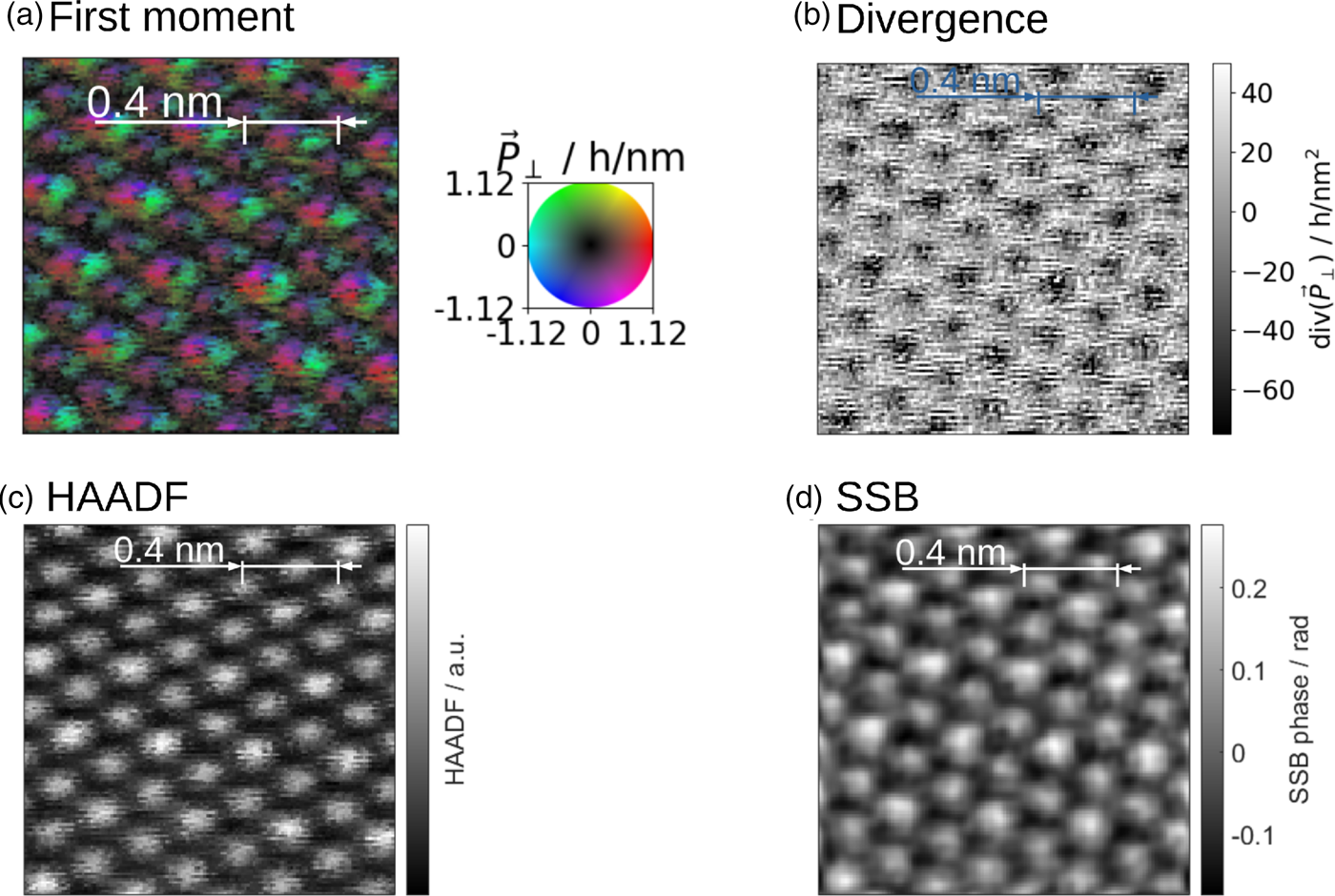
Fig. 5. Post-processing of In2Se3. In all images, the positions of the two different atom columns of In2Se3 can be seen.
In Figure 6, a comparison between different signals as well as between live imaging and post-processing of SrTiO3 is shown. Strontium titanate enables the evaluation of the different imaging modes regarding their capability for simultaneous imaging of light oxygen columns and comparably heavy Sr and Ti oxide columns, adding to the results obtained for In2Se3 in Figure 5. The first moment vector field (Fig. 6a) predominantly shows the heavy atom columns as sinks. The fact that this vector field also contains sinks at the oxygen sites becomes visible in the divergence map in Figure 6b, whereas the HAADF signal recorded separately with the conventional annular detector in Figure 6c visualizes only the heavy-atom sites of Sr and Ti oxide. In the post-processed SSB (Fig. 6d), the oxygen columns can be easily determined simultaneously with the heavy sites. The live SSB (Fig. 6g) has some noise, but the oxygen columns are still visible. Moreover, a comparison of the conventional HAADF in Figure 6c with the annular dark-field signal generated by a virtual annular detector applied to the 4D-STEM data in Figure 6f demonstrates that practically all main contrast mechanisms exploiting low- as well as high-angle scattering can be captured by the 4D-STEM imaging mode.
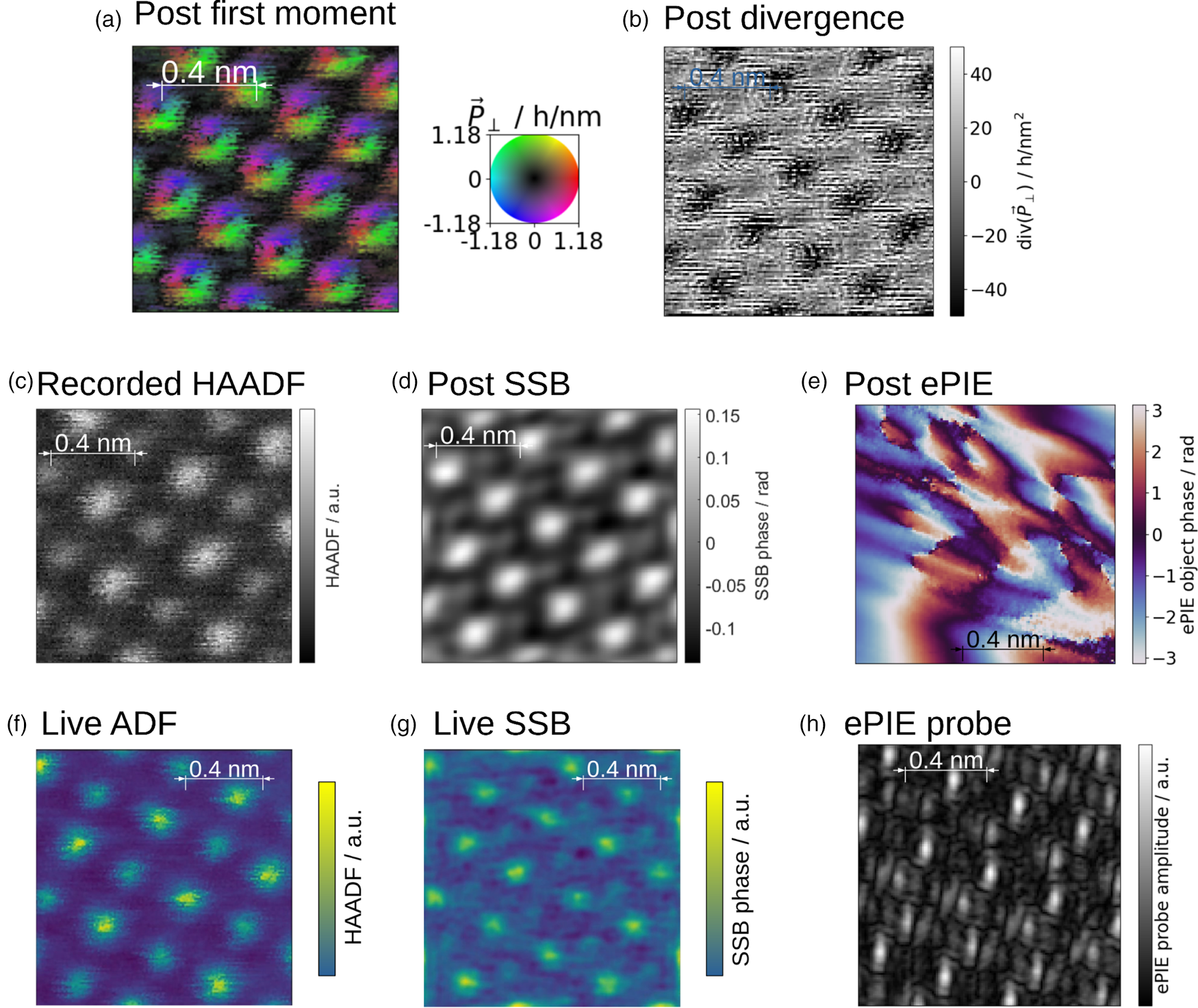
Fig. 6. Comparison between live imaging and post-processing on SrTiO3. In all images except (e), the positions of the strontium and the titanium oxide atom columns are clearly visible. The position of the oxygen columns can only be seen in the SSB results (d,g) and in the divergence of the first moment (b). The ePIE result does not show any information in the phase object. (h) The amplitude of the probe from the ePIE reconstruction shows some lattice information. The ePIE reconstruction has a 4° rotation compared with the other post-processed results due to the rotation angle. This owes to the implementation of dealing with the scan rotation. The semi-convergence angle was 22.1 mrad, the sample thickness was approximately 25 nm, determined by comparing the PACBED with simulation as shown in Figure 7.
Earlier we stated that the live ptychographic reconstruction exploits the SSB algorithm, because it is a noniterative, linear and direct scheme that allows for in situ processing. However, the weak phase object interaction model given by equation (1) is a seemingly drastic limitation of this approach. In the analysis of post-processing data, it is beneficial to explore whether a ptychographic scheme based more on an advanced interaction model, neglecting computational hardware constraints for the moment, could have been the better choice for live ptychography. To this end, we used the ePIE algorithm to reconstruct the SrTiO3 data as shown in Figure 6e. The standard ePIE implementation clearly does not give a reasonable result, at least for the usual reconstruction settings reported in the literature that we used here. To explore this in more detail, the sample thickness was determined to approximately 25 nm by comparing the experimental position averaged convergent beam electron diffraction (PACBED) with a thickness-dependent simulation as in Figure 7. Consequently, the specimen thickness was far beyond the validity of both the weak phase object approximation and the single-slice model used in ePIE. At first sight, it is nevertheless surprising that the latter approach performs worse, since one must consider it more advanced than the weak phase model from the viewpoint of scattering theory. In fact, ePIE tries to iteratively find both the probe and the object transmission function in such a way that the modulus of the Fourier transform of their product agrees best with all details of the experimental diffraction data. When dynamical scattering sets in, this multiplicative interaction scheme is incapable of delivering the details of the diffraction pattern, so that the algorithm does not converge to a reliable solution. In this particular case, ePIE has put some lattice information in the probe (Fig. 6h). This will be studied in the next subsection by means of simulations.

Fig. 7. Comparison of the PACBED of the scan in Figure 6 with simulation: The best match is achieved at a simulated thickness of 25 nm.
To summarize the experimental results, performing live ptychography using the SSB method had originally been motivated by computational aspects, but, contrary to expectations, it also turns out to be more robust against the violation of the weak phase object approximation and dynamical scattering. Of course, this only holds for qualitative imaging, but it is a significant advantage in practice where suitable structural contrast is obtained also at elevated specimen thickness for both light and heavy atomic columns.
Simulation Studies
Partial Reconstruction
As the implementation of live ptychography based on equation (3) maps the result of single scan points successively to the final reconstruction, a simulation study has been conducted in which we investigated the accuracy of the reconstructed phase in already scanned regions in dependence of the scan progress. A synthetic data set has been simulated, based on an SrTiO3 unit cell as a starting point. Then, a five by five super cell was created by repetition and the phase grating (Fig. 8) has been calculated. Two artificial spatial frequencies were added to the phase grating, one with a wavelength of a single unit cell and one with a wavelength of the super cell. To eliminate dynamical scattering in this conceptual study, a 4D-STEM simulation with 20 × 20 scan points per unit cell was performed using only one slice with a thickness of one unit cell along electron beam direction [001]. Finally, partial SSB reconstructions have been performed using the full range of scan pixels in vertical directions, but only portions of 20 scan pixels horizontally, mimicking a reconstruction during progressive scanning as depicted in Figure 9. An animation calculated from 100 single pixel columns is available in the Supplementary material.

Fig. 8. Phase grating that was used for the simulation for the partial SSB-reconstructions in Figure 9.

Fig. 9. Visualization of accumulation of partial reconstructions using a synthetic data set of simulated SrTiO3 combined with long-range potential modulation. The left column shows the reconstruction of disjoint subsets of the input data, and the right one the accumulated result until all data is processed and the complete result is obtained. An animation with smaller subdivisions is available in the Supplementary material.
Figure 9 contains the individual blocks of the 20 scan pixel wide reconstructions in the left-hand column, and the accumulated result on the right-hand side with the scan progressing from top to bottom. Consequently, the phase bottom right is the final reconstruction for the full scan, obtained by our cumulative approach which we found to be identical to a reconstruction using the conventional treatment employing the whole 4D scan. Only here, the low, medium, and atomic-scale spatial frequencies are reconstructed correctly without artifacts. In that respect, it is instructive to explore the partial reconstructions in Figure 9. Since we used subsets that equal the size of a single unit cell, spatial frequencies down to the synthetic one with a period of one unit cell appear at least qualitatively in all partial reconstructions. The sharp edges between the available data and the yet-missing region have resulted in a ringing effect near the edges known as the Gibbs-phenomenon. A closer look at the left column of Figure 9 exhibits that these artifacts largely interfere destructively during accumulation as seen, for example by a maximum at horizontal scan pixel 20 in the top row and a minimum at this position in the row below. Consequently, ringing artifacts become less obvious in the full reconstruction on the right within the region that has already been scanned. Therefore, it is already possible to visualize the atomic structure and partly meso-scale phase variations for partial scans, making it possible to navigate on the sample and visually interpret results in a real experiment.
Real specimens and scan regions do not usually fulfill periodic boundary conditions which still apply to the full scan of Figure 9. Therefore, Figure 10 shows the impact of selecting different reconstruction areas by simulating the reconstruction of a smaller scan area that is not aligned with the underlying lattice. SSB reconstructs the specimen with an assumption of a periodic boundary condition and cannot reconstruct spatial frequencies above a certain threshold, as previously discussed. Trying to reconstruct a field of view where wrapping around the edges creates a discontinuity, that is frequencies higher than SSB can reconstruct, leads to reconstruction artifacts as seen in Figure 9. Quantitatively, the difference between the ground truth taken from the marked rectangle of the full reconstruction in Figure 10a and a reconstruction that solely employs the scan pixels therein, as seen in Figure 10b is mapped in Figure 10c and can take significant values of 5–10% of the phase itself in the present example.
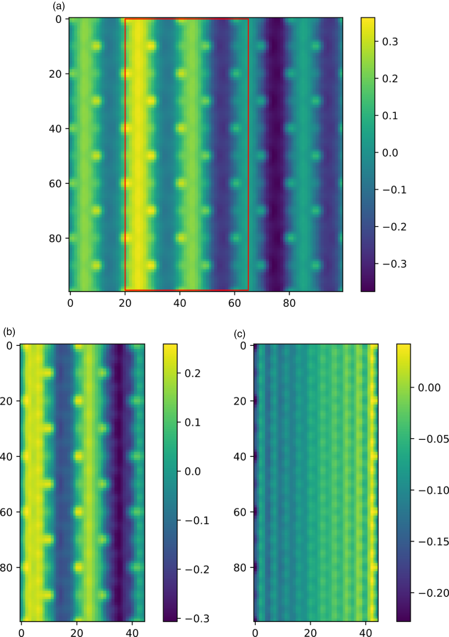
Fig. 10. Reconstruction limited to a cutout from the data in both reconstructed area and input data, as opposed to partial reconstruction of the area of the full data set in Figure 9. (a) The selected cutout area from the full reconstruction, (b) the reconstruction limited to this area, and (c) the difference between the two. This demonstrates how a discontinuity from wrapping around at the edges for a periodic boundary condition creates reconstruction artifacts due to the high-frequency cutoff of SSB.
As a solution, the field of view where an accurate reconstruction is required can be surrounded by a smooth transition to a zero-valued buffer area so that the presence of spatial frequencies above the resolution limit is minimized when the reconstruction area is wrapped around at the edges. In future studies, a Lanczos filtering (Duchon, Reference Duchon1979) scheme could be added for our live ptychography approach.
Thickness Effects
A comprehensive algorithmic review is not our focus but touching briefly on the findings in conjunction with Figure 6 we elucidate the impact of dynamical scattering, or, equivalently, specimen thickness, on different signals. A multislice simulation (Rosenauer & Schowalter, Reference Rosenauer and Schowalter2007) has been performed for SrTiO3 in [001] projection employing the experimental parameters and using 20 × 20 scan pixels. The data were evaluated for thicknesses of 1 and 30 nm, addressing both the kinematic case and the situation of elevated thickness in our experiment. The results have been compiled in Figure 11.
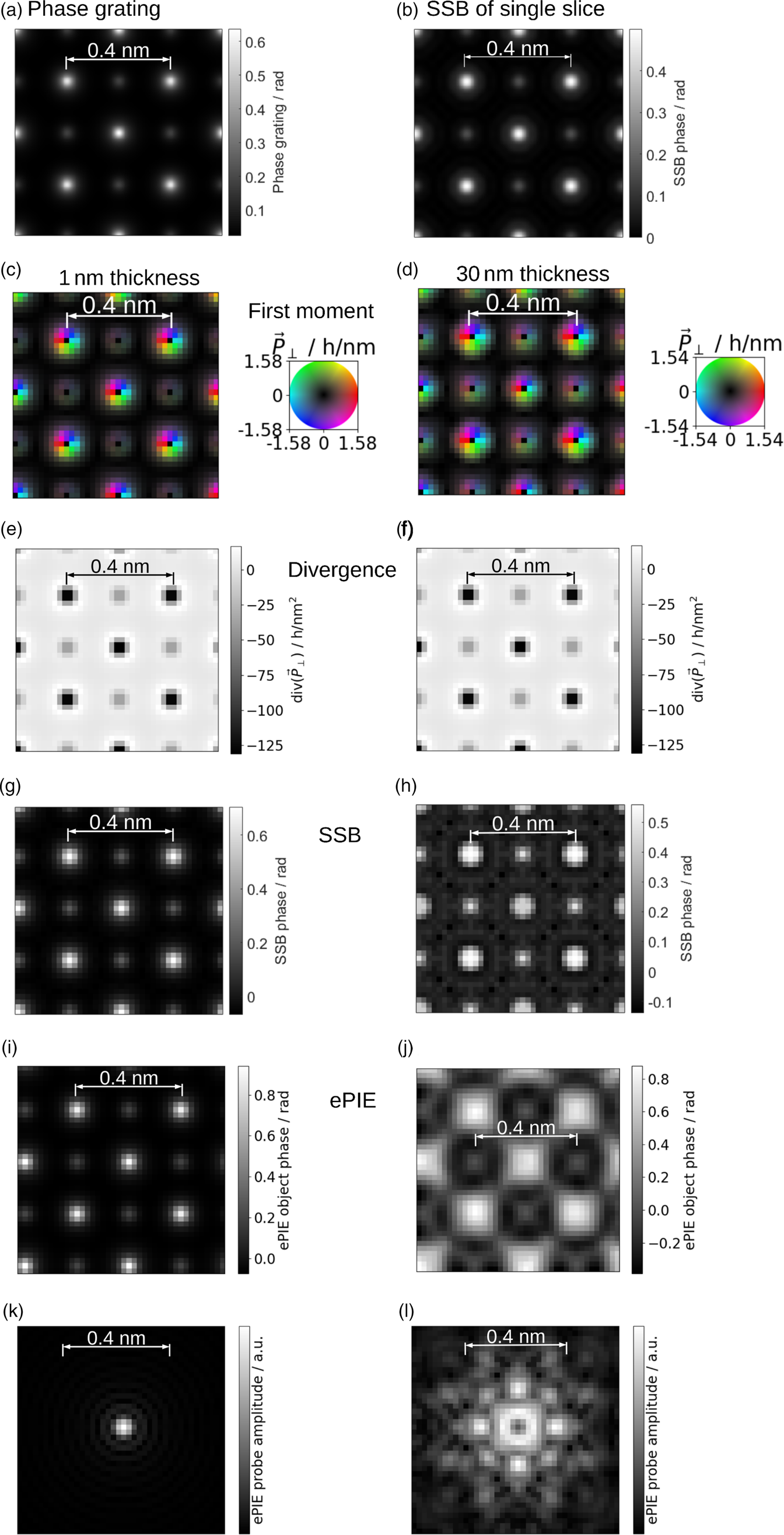
Fig. 11. Simulations for SrTiO3: (a) Phase grating used for multislice simulation, (b) SSB from a single slice simulation using also the weak phase approximation in the simulation, (c,d) First moment, (e,f) Divergence of first moment, (g,h) SSB without using weak phase approximation in the simulation of the 4D-STEM-data, (i,j) phase object from ePIE, (k,l) probe amplitude from ePIE, (c,e,g,i,k) 1 nm sample thickness, and (d,f,h,j,l) 30 nm sample thickness. The simulation parameters where chosen to match those used in the experiments. Additionally, the following parameters were used: 22.1 mrad semi-convergence angle and 20 by 20 scan points per unit cell.
Figure 11a shows the phase grating used in the multislice simulation for structural reference. In Figure 11b, we added the theoretical result that would be obtained for SSB ptychography in case all methodological premises were fulfilled in practice. That is, we generated a 4D-STEM data set by means of the weak phase approximation in equation (1) for a single slice with the thickness of one SrTiO3 unit cell and performed the SSB reconstruction. Note that this is identical to the phase Φ in equation (1), low-pass filtered with a circular aperture that has twice the radius of the probe-forming aperture.
Figures 11c–11j show the results of evaluating the 1 nm (left column) and the 30 nm data (right column) using different methods aligned row-wise. As can be expected from former studies employing first moment-based imaging (Müller et al., Reference Müller, Krause, Beche, Schowalter, Galioit, Löffler, Verbeeck, Zweck, Schattschneider and Rosenauer2014; Müller-Caspary et al., Reference Müller-Caspary, Krause, Grieb, Löffler, Schowalter, Béché, Galioit, Marquardt, Zweck, Schattschneider, Verbeeck and Rosenauer2017) of centrosymmetric structures, Figures 11c–11f resemble the atomic structure in terms of momentum transfer vector maps and their divergences with the atoms being sites of central fields. This is preserved in qualitative manner only for more elevated thicknesses. Note that Figures 11c and 11e are proportional to the probe-convoluted distributions of the projected electric field and charge density, respectively.
Similarly, the SSB reconstructions in Figures 11g and 11h yield reliable structural contrast at both low and elevated thickness despite the violation of the weak phase approximation in equation (1), which confirms our interpretation in the post-processing section. However, already the result in Figure 11g should be considered as qualitative except for the oxygen sites. Note that the probe had been focused on the specimen surface in the simulation. Because the SSB reconstruction considers the 30 nm thick specimen as a single slice here, the optimum focus would have been at some depth inside the specimen which is one reason why atomic sites appear slightly broader (Fig. 11h).
The situation is different for the ePIE results in Figures 11i and 11j. Whereas the reconstruction for the thin specimen in Figure 11i represents the phase excellently and can be considered quantitative within the general framework of validity of ePIE, the algorithm has severe difficulties in reconstructing the object transmission function at 30 nm thickness in Figure 11j. In Figure 11k, the reconstructed probe looks like an airy disc. This is the result of an aberration-free probe, limited only by an aperture in diffraction space, and that was used in the simulation. In Figure 11l, sample information is transferred to the probe. This further confirms our observations concerning ePIE in the post-processing section by simulation. However, Figures 6e, 6h give even less information from the specimen than Figures 11j, 11l, which can be attributed to Poisson noise neglected in the simulation, residual aberrations, and importantly, different manners of separating probe and object which starts to fail when dynamical scattering sets in. To conclude, selecting the SSB scheme for live imaging of structural contrast can also be supported from the simulation point of view.
Low Dose
The performance of the SSB reconstruction and the divergence of the first moment was checked in a low-dose simulation (Fig. 12). At 1,000 electrons per Å2 (Figs. 12a, 12b), the heavy-atom columns are visible. At this dose, the SSB reconstruction gives stronger contrast than the divergence of the first moment. At 10,000 electrons per Å2 (Figs. 12c, 12d), also the oxygen atom columns are visible. The SSB reconstruction and the divergence of the first moment shows similar performance at this dose.
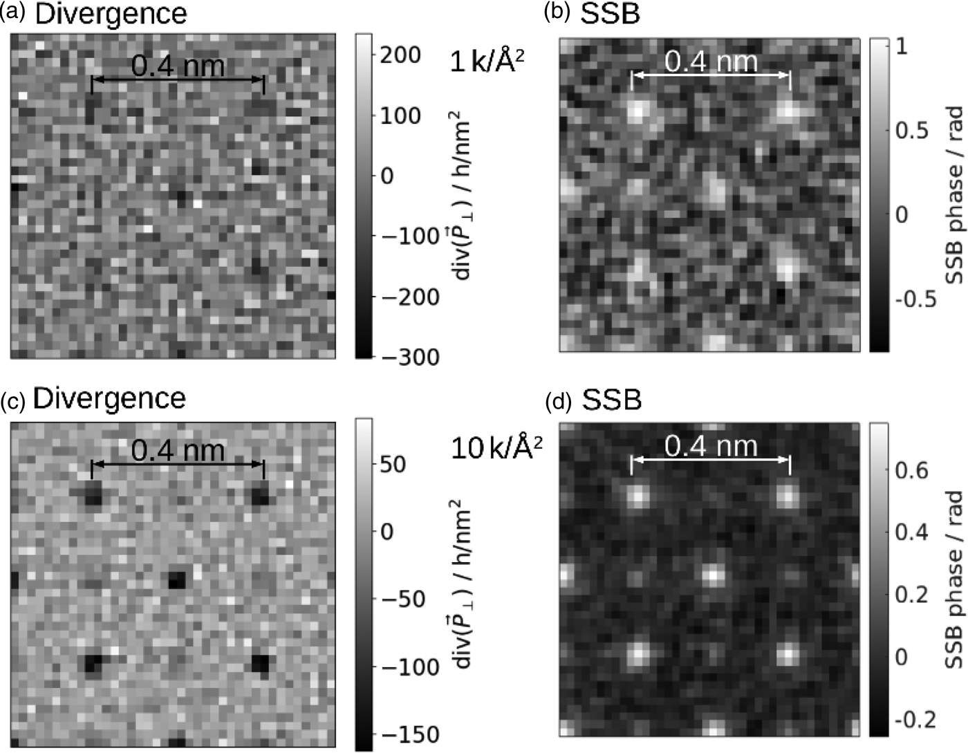
Fig. 12. Low dose simulation for SrTiO3: (a,c) Divergence of first moment, (b,d) SSB without using weak phase approximation in the simulation of the 4D-STEM-data, (a,b) at 1,000 electrons per Å2 and (c,d) at 10,000 electrons per Å2. The simulation parameters where the same as in Figure 11c.
Discussion
The digitization that took place decades ago with key developments such as charge-coupled device (CCD) cameras and computer controlling, processing and visualization in STEM denotes one of the drastic paradigm changes in electron microscopy. It enabled the live assessment of recorded data and transformed an optimization of experimental parameters from multiple sessions to a quick feedback loop taking only several minutes within a single session. Surprisingly, innovative hardware associated with an increase of the dimensionality of the recorded data has, to some extent, put us back to ancient workflows for advanced methodologies. A major challenge for contemporary imaging in the era of Big Data is, thus, to make current ex situ multidimensional evaluations capable for live imaging. Within this context, the present work shall be seen as a first step that demonstrates the feasibility of such a workflow using a rather straightforward example. Our work highlights the ongoing push toward high-performance computational methods in electron microscopy that are driven by an increasing camera performance (Weber et al., Reference Weber, Clausen and Dunin-Borkowski2020). That includes suitable software frameworks, connections, storage, processing hardware, and know-how in computer science and engineering to be used in synergy with established and future imaging methodologies.
Several important general conclusions can be drawn from the present study. First, adequate computational hardware is already available for this purpose, given that the mathematical formulation can be adapted to make use of it efficiently. Second, and most importantly, open and well-defined software interfaces which were available for the hardware used here, are key prerequisites to implement nonstandard imaging concepts developed in science into established infrastructures. Third, it can be beneficial to exploit partly simplistic models to achieve live imaging capabilities, exemplified here by the use of the SSB algorithm for a materials science case. On the one hand, it violates inherent assumptions significantly; on the other hand, the qualitative nature of the results is better than one might expect from the weak phase approximation. In particular, the present setup can be considered to be highly beneficial for low-dose ptychographic live imaging of challenging specimen in the fields of structural biology and soft matter in Cryo electron microscopy. A suitable experimental setup with open software interfaces to tap the data stream of a 4D-Cryo-STEM experiment was unfortunately not available to the authors to enable the inclusion of respective examples in the present report. On the other hand, this would not change the methodological setup worked out in this paper using solid-state examples.
The current implementation mainly served to investigate the fundamental feasibility and characteristics of ptychography for live imaging. Integrating the parameter selection and results display in to existing instrument control software could be the next steps to improve the usability, making it more practical to apply routinely in microscopy. In that respect, live focusing, stigmation, and, prospectively, correction of further aberrations based on ptychography are possible. Furthermore, the implementation can be extended to include mitigation of artifacts from the edges that are demonstrated in Figure 10.
Existing LiberTEM UDFs that were previously only used for offline processing were applied to live data without modification, proving a long-standing design goal of LiberTEM (Clausen et al., Reference Clausen, Weber, Ruzaeva, Migunov, Baburajan, Bahuleyan, Caron, Chandra, Halder, Nord, Müller-Caspary and Dunin-Borkowski2020b). In particular, the UDF interface allowed to disentangle details of the data logistics from the numerical and scientific aspects of the used algorithms. The prototype data decoder and UDF runner could easily keep up with the data rate of the Merlin detector. UDFs with low computational load such as virtual detectors or first moments remained at single-digit CPU load percentages. That means much higher data rates are likely to be possible with a suitable distributed UDF runner implementation. This will be required to support multi-chip cameras such as the Gatan K2 or K3 IS or X-Spectrum Lambda. Computationally intensive operations like ptychography are more challenging to scale to such data rates.
The poor scaling behavior of the current SSB implementation has proven to be a limiting factor. For illustration, doubling the scan resolution at constant aspect ratio quadruples the number of scan points and results in 16x increased computation time. In future, an implementation that significantly reduces the computational load would be highly desirable to make this technique useful for mainstream data analysis. Ideally, there would be a constant memory consumption independent of scan area and  ${\cal O}( N)$ or ${\cal O}( N \log N)$ scaling for computation effort as a function of the number of scan points.
Summary
Live imaging of central 4D-STEM signals such as the ptychographic phase, first moments, their divergence and rotation, as well as flexible virtual detectors has been demonstrated. A direct processing of the data stream of a Medipix3 chip mounted in an aberration-corrected STEM was implemented. An enhanced version is available open-source under https://github.com/LiberTEM/LiberTEM-live. A prototype was used to generate the live results and is available upon request. The live imaging capability could be demonstrated for two materials science cases In2Se3 and SrTiO3, where single-sideband ptychography proved surprisingly robust against imaging at elevated specimen thicknesses around 20 nm. It is anticipated that the live imaging approach presented here, and the transfer of such direct workflows to further imaging methods, can also enhance imaging in life sciences where, for example, ptychography is a promising candidate for high-contrast, low-dose imaging of weakly scattering objects without compromising spatial resolution.
Supplementary material
To view supplementary material for this article, please visit https://doi.org/10.1017/S1431927621012423.
Acknowledgments
Knut Müller-Caspary, Achim Strauch, and Benjamin März were supported by funding from the Initiative and Network Fund of the Helmholtz Association (Germany) under contract VH-NG-1317 (moreSTEM project). Dieter Weber, Alexander Clausen, Arya Bangun, Benjamin März, and Knut Müller-Caspary acknowledge support from Helmholtz within the project “Ptychography 4.0” under contract ZT-I-0025. Dieter Weber, Alexander Clausen, and Rafal Dunin-Borkowski received funding from the European Union's Horizon 2020 research and innovation programme under grant agreements No. 823717 – ESTEEM3 and No. 780487 – VIDEO.


 Open access