


1. Introduction
The $\lambda$
-calculus has been historically conceived as an equational theory of functions, so that reduction had an ancillary role in Church’s view, and it was a tool for studying the theory
$\lambda$
-calculus has been historically conceived as an equational theory of functions, so that reduction had an ancillary role in Church’s view, and it was a tool for studying the theory $\beta$
, see Barendregt (Reference Barendregt1984, Ch. 3). The development of functional programming languages like Lisp and ML, and of proof assistants like LCF, has brought a new, different interest in the
$\beta$
, see Barendregt (Reference Barendregt1984, Ch. 3). The development of functional programming languages like Lisp and ML, and of proof assistants like LCF, has brought a new, different interest in the $\lambda$
-calculus and its reduction theory.
$\lambda$
-calculus and its reduction theory.
The cornerstone of this change in perspective is Plotkin’s (1975), where the functional parameter passing mechanism is formalized by the call-by-value rewrite rule $\beta_v$
, allowing reduction only if the argument term is a value, that is a variable or an abstraction. In Plotkin (Reference Plotkin1975), it is also introduced the notion of weak evaluation, namely no reduction in the body of a function (i.e., of an abstraction).
$\beta_v$
, allowing reduction only if the argument term is a value, that is a variable or an abstraction. In Plotkin (Reference Plotkin1975), it is also introduced the notion of weak evaluation, namely no reduction in the body of a function (i.e., of an abstraction).
This is now the standard evaluation implemented by functional programming languages, where values are the terms of interest (and the normal forms for weak evaluation in the closed case). Full $\beta_v$
reduction is instead the basis of proof assistants like Coq, where normal forms are the result of interest. More generally, the computational perspective on
$\beta_v$
reduction is instead the basis of proof assistants like Coq, where normal forms are the result of interest. More generally, the computational perspective on $\lambda$
-calculus has given a central role to reduction, whose theory provides a sound framework for reasoning about program transformations, such as compiler optimizations or parallel implementations.
$\lambda$
-calculus has given a central role to reduction, whose theory provides a sound framework for reasoning about program transformations, such as compiler optimizations or parallel implementations.
The rich variety of computational effects in actual implementations of functional programming languages brings further challenges. This dramatically affects the theory of reduction of the calculi formalizing such features, whose proliferation makes it difficult to focus on suitably general issues. A major change here is the discovery by Moggi (Reference Moggi1988, 1989, Reference Moggi1991) of a whole family of calculi that are based on a few common traits, combining call-by-value with the abstract notion of effectful computation represented by a monad, which has shown to be quite successful. But Moggi’s computational $\lambda$
-calculus is an equational theory in the broader sense; much less is known of the reduction theory of such calculi: this is the focus of our paper.
$\lambda$
-calculus is an equational theory in the broader sense; much less is known of the reduction theory of such calculi: this is the focus of our paper.
The Computational Calculus. Since Moggi’s seminal work, computational $\lambda$
-calculi have been developed as a foundation of programming languages, formalizing both functional and non-functional features, see e.g. Wadler and Thiemann (Reference Wadler and Thiemann2003), Benton et al. (Reference Benton, Hughes and Moggi2002), starting a thread in the literature that is still growing. The basic idea of computational
$\lambda$
-calculi have been developed as a foundation of programming languages, formalizing both functional and non-functional features, see e.g. Wadler and Thiemann (Reference Wadler and Thiemann2003), Benton et al. (Reference Benton, Hughes and Moggi2002), starting a thread in the literature that is still growing. The basic idea of computational $\lambda$
-calculi is to distinguish values and computations, so that programs, represented by closed terms, are thought of as functions from values to computations. Intuitively, computations embody a richer structure than values and do form a larger set in which values can be embedded. On the other hand, the essence of programming is composition; to compose functions from values to computations we need a mechanism to uniformly extend them to functions of computations, while preserving their original behavior over the (image of) values.
$\lambda$
-calculi is to distinguish values and computations, so that programs, represented by closed terms, are thought of as functions from values to computations. Intuitively, computations embody a richer structure than values and do form a larger set in which values can be embedded. On the other hand, the essence of programming is composition; to compose functions from values to computations we need a mechanism to uniformly extend them to functions of computations, while preserving their original behavior over the (image of) values.
To model these concepts, Moggi used the categorical notion of monad, abstractly representing the extension of the space of values to that of computations, and the associated Kleisli category, whose morphisms are functions from values to computations, which are the denotations of programs. Syntactically, following Wadler (Reference Wadler1995), we can express these ideas by means of a call-by-value $\lambda$
-calculus with two sorts of terms: values, ranged over by V,W, namely variables or abstractions, and computations denoted by L,M,N. Computations are formed by means of two operators: values are embedded into computations by means of the operator
$\lambda$
-calculus with two sorts of terms: values, ranged over by V,W, namely variables or abstractions, and computations denoted by L,M,N. Computations are formed by means of two operators: values are embedded into computations by means of the operator $ unit$
written return in Haskell programming language, whose name refers to the unit of a monad in categorical terms; a computation
$ unit$
written return in Haskell programming language, whose name refers to the unit of a monad in categorical terms; a computation
![]() is formed by the binary operator
is formed by the binary operator
![]() , called bind (
, called bind ( $\texttt{>>=}$
in Haskell), representing the application to M of the extension to computations of the function
$\texttt{>>=}$
in Haskell), representing the application to M of the extension to computations of the function $\lambda x.N$
.
$\lambda x.N$
.
The Monadic Laws. The operational understanding of these new operators is that evaluating
![]() , which in Moggi’s notation reads
, which in Moggi’s notation reads
![]() , amounts to first evaluating M until a computation of the form
, amounts to first evaluating M until a computation of the form
![]() is reached, representing the trivial computation that returns the value V. Then V is passed to N by binding x to V, as expressed by the identity:
is reached, representing the trivial computation that returns the value V. Then V is passed to N by binding x to V, as expressed by the identity:
This is the first of the three monadic laws in Wadler (Reference Wadler1995). The remaining laws are
To understand these two last rules, let us define the composition (named Kleisli composition in category theory) of the functions
![]() and
and
![]() as
as
where we can freely assume that x is not free in N.
Equality (2) (identity) implies that
![]() , which paired with the instance of (1):
, which paired with the instance of (1):
![]() (where
(where
![]() is the usual congruence generated by the renaming of bound variables), tells that
is the usual congruence generated by the renaming of bound variables), tells that
![]() is the identity of composition
is the identity of composition
![]() .
.
Equality (3) (associativity) implies:
namely that composition
![]() is associative.
is associative.
The monadic laws correspond to the three equalities in the definition of a Kleisli triple (Moggi Reference Moggi1991), which is an equivalent presentation of monads (MacLane Reference MacLane1997). Indeed, Moggi’s calculus is the internal language of a suitable category equipped with a (strong) monad T, and with enough structure to internalize the morphisms of the respective Kleisli category. As such, it is a simply typed
![]() -calculus, where T is the type constructor associating with each type A the type TA of computations over A. Therefore,
-calculus, where T is the type constructor associating with each type A the type TA of computations over A. Therefore,
![]() and
and
![]() are polymorphic operators with respective types (Wadler Reference Wadler1992, Reference Wadler1995):
are polymorphic operators with respective types (Wadler Reference Wadler1992, Reference Wadler1995):
The Computational Core. The dynamics of
![]() -calculi is usually defined as a reduction relation on untyped terms. Moggi’s preliminary report (Moggi Reference Moggi1988) specifies both an equational and, in Section 6, a reduction system even if only the former is thoroughly investigated and appears in (Moggi Reference Moggi1989, Reference Moggi1991), while reduction is briefly treated for an untyped fragment of the calculus. However, when stepping from the typed calculus to the untyped one, we need to be careful by avoiding meaningless terms to creep into the syntax, so jeopardizing the calculus theory. For example: what should be the meaning of
-calculi is usually defined as a reduction relation on untyped terms. Moggi’s preliminary report (Moggi Reference Moggi1988) specifies both an equational and, in Section 6, a reduction system even if only the former is thoroughly investigated and appears in (Moggi Reference Moggi1989, Reference Moggi1991), while reduction is briefly treated for an untyped fragment of the calculus. However, when stepping from the typed calculus to the untyped one, we need to be careful by avoiding meaningless terms to creep into the syntax, so jeopardizing the calculus theory. For example: what should be the meaning of
![]() where both M and N are computations? What about
where both M and N are computations? What about
![]() for any V? Shall we have functional applications of any kind?
for any V? Shall we have functional applications of any kind?
To answer these questions, in de' Liguoro and Treglia (2020) typability is taken as syntactic counterpart of being meaningful: inspired by ideas in Scott (Reference Scott, Hindley and Seldin1980), the untyped computational
![]() -calculus is a special case of the typed one, where there are just two types D and TD, related by the type equation
-calculus is a special case of the typed one, where there are just two types D and TD, related by the type equation
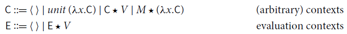
![]() , that is Moggi’s isomorphism of the call-by-value reflexive object (see Moggi Reference Moggi1988, Section 5). With such a proviso, we get the following syntax:
, that is Moggi’s isomorphism of the call-by-value reflexive object (see Moggi Reference Moggi1988, Section 5). With such a proviso, we get the following syntax:
If we assume that all variables have type D, then it is easy to see that all terms in
![]() have type
have type
![]() , which is consistent with the substitution of variables with values in (1). On the other hand, considering the typing of
, which is consistent with the substitution of variables with values in (1). On the other hand, considering the typing of
![]() and
and
![]() in (4), terms in
in (4), terms in
![]() have type TD. As we have touched above, there is some variety in notation among computational
have type TD. As we have touched above, there is some variety in notation among computational
![]() -calculi; we choose the above syntax because it explicitly embodies the essential constructs of a
-calculi; we choose the above syntax because it explicitly embodies the essential constructs of a
![]() -calculus with monads, but for functional application, which is definable: see Section 3 for further explanations. We dub the calculus computational core, noted
-calculus with monads, but for functional application, which is definable: see Section 3 for further explanations. We dub the calculus computational core, noted
![]() .
.
From Equalities to Reduction. Similarly to Moggi (Reference Moggi1988) and Sabry and Wadler (Reference Sabry and Wadler1997), the reduction rules in the computational core
![]() are the relation obtained by orienting the monadic laws from left to right. We indicate by
are the relation obtained by orienting the monadic laws from left to right. We indicate by
![]() ,
,
![]() , and
, and
![]() the rules corresponding to (1), (2), and (3), respectively. The contextual closure of these rules, noted
the rules corresponding to (1), (2), and (3), respectively. The contextual closure of these rules, noted
![]() , has been proved confluent in de' Liguoro and Treglia (2020), which implies that equal terms have a common reduct and the uniqueness of normal forms.
, has been proved confluent in de' Liguoro and Treglia (2020), which implies that equal terms have a common reduct and the uniqueness of normal forms.
In Plotkin (Reference Plotkin1975) call-by-value reduction
![]() is an intermediate concept between the equational theory and the evaluation relation
is an intermediate concept between the equational theory and the evaluation relation
![]() , that models an abstract machine. Evaluation consists of persistently choosing the leftmost
, that models an abstract machine. Evaluation consists of persistently choosing the leftmost
![]() -redex that is not in the scope of an abstraction, i.e., evaluation is weak.
-redex that is not in the scope of an abstraction, i.e., evaluation is weak.
The following crucial result bridges reduction (hence, the foundational calculus) with evaluation (implemented by an ideal programming language):
Such a result (Corollary 1 in Plotkin Reference Plotkin1975) comes from an analysis of the reduction properties of
![]() , namely standardization.
, namely standardization.
As we will see, the rules induced by associativity and identity make the behavior of the reduction in
![]() – and the study of its operational properties – nontrivial in the setting of any monadic
– and the study of its operational properties – nontrivial in the setting of any monadic
![]() -calculus. The issues are inherent to the rules coming from the monadic laws (2) and (3), independently of the syntactic representation of the calculus that internalizes them. The difficulty appears clearly if we want to follow a similar route to Plotkin (Reference Plotkin1975), as we discuss next.
-calculus. The issues are inherent to the rules coming from the monadic laws (2) and (3), independently of the syntactic representation of the calculus that internalizes them. The difficulty appears clearly if we want to follow a similar route to Plotkin (Reference Plotkin1975), as we discuss next.
Reduction vs. Evaluation. Following Felleisen (Reference Felleisen1988), reduction
![]() and evaluation
and evaluation
![]() of
of
![]() can be defined as the closure of the reduction rules under arbitrary and evaluation contexts, respectively. Consider the following grammars:
can be defined as the closure of the reduction rules under arbitrary and evaluation contexts, respectively. Consider the following grammars:
where the hole
![]() can be filled by terms in
can be filled by terms in
![]() , only. Observe that the closure under evaluation context
, only. Observe that the closure under evaluation context
![]() is precisely weak reduction.
is precisely weak reduction.
Weak reduction of
![]() , however, turns out to be nondeterministic, nonconfluent, and its normal forms are not unique. The following is a counterexample to all such properties – see Section 5 for further examples.
, however, turns out to be nondeterministic, nonconfluent, and its normal forms are not unique. The following is a counterexample to all such properties – see Section 5 for further examples.
Such an issue is not specific to the syntax of the computational core . The same phenomena show up with the let-notation, more commonly used in computational calculi. Here, evaluation, usually called sequencing, is the reduction defined by the following contexts (Filinski Reference Filinski1996; Jones et al. Reference Jones, Shields, Launchbury, Tolmach, MacQueen and Cardelli1998; Levy et al. Reference Levy, Power and Thielecke2003):
Examples similar to the one above can be reproduced. We give the details in Example 5.3.
1.1 Content and contributions
The focus of this paper is an operational analysis of two crucial properties of a term M:
(i). M returns a value ( i.e.
![]() , for some V value).
, for some V value).
(ii). M has a normal form ( i.e.
![]() , for some N
, for some N
![]() -normal).
-normal).
As in Accattoli et al. (Reference Accattoli, Faggian and Guerrieri2019), the cornerstone of our analysis are factorization results (also called semi-standardization in the literature): any reduction sequence can be reorganized so as to first performing specific steps and then everything else.
Via factorization, we show the key result (6), analogous to (5), relating reduction and evaluation:
We then analyze the property of having a normal form (normalization), and define a family of normalizing strategies, i.e., subreductions that are guaranteed to reach a normal form, if any exists.
On the Rewrite Theory of Computational Calculi. In this paper, we study the rewrite theory of a specific computational calculus, namely
![]() . We expose a number of issues, which we argue to be intrinsic to the monadic rules of computational calculi, namely associativity and identity. Indeed, the same issues which we expose in
. We expose a number of issues, which we argue to be intrinsic to the monadic rules of computational calculi, namely associativity and identity. Indeed, the same issues which we expose in
![]() , also appear in other computational calculi, as we discuss in Section 5, where we take as reference the calculus in Sabry and Wadler (Reference Sabry and Wadler1997), which we recall in Section 3.1. We expect that the solutions we propose for
, also appear in other computational calculi, as we discuss in Section 5, where we take as reference the calculus in Sabry and Wadler (Reference Sabry and Wadler1997), which we recall in Section 3.1. We expect that the solutions we propose for
![]() could be adapted also there.
could be adapted also there.
Surface Reduction. The form of weak reduction that we defined in the previous section (sequencing) is standard in the literature. In this paper, we study also a less strict form of weak reduction, namely surface reduction, which is less constrained and better behaved then sequencing. Surface reduction disallows reduction under the
![]() operator only, and not under abstractions. Intuitively, weak reduction does not act in the body of a function, while surface reduction does not act in the scope of return. As we discuss in Section 3.1, it can also be seen as a more natural extension of call-by-value weak reduction to a computational calculus.
operator only, and not under abstractions. Intuitively, weak reduction does not act in the body of a function, while surface reduction does not act in the scope of return. As we discuss in Section 3.1, it can also be seen as a more natural extension of call-by-value weak reduction to a computational calculus.
Surface reduction is well studied in the literature because it naturally arises when interpreting
![]() -calculus into linear logic, and indeed the name surface (which we take from Simpson Reference Simpson and Giesl2005) is reminiscent of a similar notion in calculi based on linear logic (Ehrhard and Guerrieri Reference Ehrhard and Guerrieri2016; Simpson Reference Simpson and Giesl2005). In Section 4, we will make explicit the correspondence with such calculi, showing that the
-calculus into linear logic, and indeed the name surface (which we take from Simpson Reference Simpson and Giesl2005) is reminiscent of a similar notion in calculi based on linear logic (Ehrhard and Guerrieri Reference Ehrhard and Guerrieri2016; Simpson Reference Simpson and Giesl2005). In Section 4, we will make explicit the correspondence with such calculi, showing that the
![]() operator (from the computational core) behaves exactly like a bang
operator (from the computational core) behaves exactly like a bang
![]() (from linear logic).
(from linear logic).
Identity and Associativity. Our analysis exposes the operational role of the rules associated to the monadic laws of identity and associativity.
(i) To compute a value, only
![]() steps are necessary.
steps are necessary.
(ii) To compute a normal form,
![]() steps do not suffice: associativity (i.e.,
steps do not suffice: associativity (i.e.,
![]() steps) is necessary.
steps) is necessary.
Hence, the rule associated to the identity law turns out to be operationally irrelevant.
Normalization. The study of normalization is more complex than that of evaluation and requires some sophisticated techniques. We highlight some specific contributions.
• We define two families of normalizing strategies in
![]() . The first one, quite constrained, relies on an iteration of weak reduction
. The first one, quite constrained, relies on an iteration of weak reduction
![]() . The second one, more liberal, is based on an iteration of surface reduction
. The second one, more liberal, is based on an iteration of surface reduction
![]() . The definition and proof of normalization is parametric on either.
. The definition and proof of normalization is parametric on either.
• The technical difficulty in the proofs for normalization comes from the fact that neither weak nor surface reduction is deterministic. To deal with that we rely on a fine quantitative analysis of the number of
![]() steps, which we carry-on when we study factorization in Section 6.
steps, which we carry-on when we study factorization in Section 6.
The most challenging proofs in the paper are those related to normalization via surface reduction. The effort is justified by the interest in a larger and more versatile strategy, which then does not induce a single abstract machine but subsumes several ones, each following a different reduction policy. It thus facilitates reasoning about optimization techniques and parallel implementation.
A Roadmap. Let us summarize the structure of the paper.
Section 2 contains the background notions which are relevant to our paper.
Section 3 gives the formal definition of the computational core
![]() and its reduction.
and its reduction.
In Sections 4 and 5, we analyze the properties of weak and surface reduction. We first study
![]() , and then we move to the whole
, and then we move to the whole
![]() , where associativity and identity also come to play, and issues appear.
, where associativity and identity also come to play, and issues appear.
In Section 6 we study several factorization results. The cornerstone of our construction is surface factorization (Theorem 6.1). We then further refine this result, first by postponing the
![]() steps which are not
steps which are not
![]() steps, and then with a form of weak factorization.
steps, and then with a form of weak factorization.
In Section 7, we study evaluation and analyze some relevant consequences of this result. We actually provide two different ways to deterministically compute a value. The first way is the one given by (6), via an evaluation context. The second way requires no contextual closure at all: simply applying
![]() - and
- and
![]() -rules will return a value, if possible.
-rules will return a value, if possible.
In Section 8 we study normalization and normalizing strategies.
Section 9 concludes with final discussions and related work.
2. Preliminaries
2.1 Basics on rewriting
We recall here some standard definitions and notations in rewriting that we shall use in this paper (see for instance Terese 2003 or Baader and Nipkow Reference Baader and Nipkow1998 for details).
Rewriting System. An abstract rewriting system (ARS) is a pair
![]() consisting of a set A and a binary relation
consisting of a set A and a binary relation
![]() on A whose pairs are written
on A whose pairs are written
![]() and called steps. A
and called steps. A
![]() -sequence from
-sequence from
![]() is a sequence
is a sequence
![]() of
of
![]() steps, where
steps, where
![]() or
or
![]() for some
for some
![]() ,
,
![]() for all
for all
![]() and
and
![]() (in particular, the sequence is empty for
(in particular, the sequence is empty for
![]() , i.e.
, i.e.
![]() ). We denote by
). We denote by
![]() (resp.
(resp.
![]() ;
;
![]() ) the transitive-reflexive (resp. reflexive; transitive) closure of
) the transitive-reflexive (resp. reflexive; transitive) closure of
![]() , and
, and
![]() stands for the transpose of
stands for the transpose of
![]() , that is,
, that is,
![]() if
if
![]() . We write
. We write
![]() for a
for a
![]() -sequence
-sequence
![]() of
of
![]() steps. If
steps. If
![]() are binary relations on
are binary relations on
![]() then
then
![]() denotes their composition, i.e.
denotes their composition, i.e.
![]() if there exists
if there exists
![]() such that
such that
![]() . We often set
. We often set
![]() .
.
A relation
![]() is deterministic if for each
is deterministic if for each
![]() there is at most one
there is at most one
![]() such that
such that
![]() . It is confluent if
. It is confluent if
![]() .
.
We say that
![]() is
is
![]() -normal (or a
-normal (or a
![]() -normal form, noted
-normal form, noted
![]() ) if
) if
![]() for all
for all
![]() , that is, there is no
, that is, there is no
![]() such that
such that
![]() ; and we say that
; and we say that
![]() has a normal form u if
has a normal form u if
![]() with u
with u
![]() -normal. Confluence implies that each
-normal. Confluence implies that each
![]() has unique normal form, if any exists.
has unique normal form, if any exists.
Normalization. Let
![]() be an ARS. In general, a term may or may not reduce to a normal form. And if it does, not all reduction sequences necessarily lead to a normal form. A term is weakly or strongly normalizing, depending on if it may or must reduce to normal form. If a term
be an ARS. In general, a term may or may not reduce to a normal form. And if it does, not all reduction sequences necessarily lead to a normal form. A term is weakly or strongly normalizing, depending on if it may or must reduce to normal form. If a term
![]() is strongly normalizing, any choice of steps will eventually lead to a normal form. However, if
is strongly normalizing, any choice of steps will eventually lead to a normal form. However, if
![]() is weakly normalizing, how do we compute a normal form? This is the problem tackled by normalization and normalizing strategies: by repeatedly performing only specific steps, a normal form will be computed, provided that
is weakly normalizing, how do we compute a normal form? This is the problem tackled by normalization and normalizing strategies: by repeatedly performing only specific steps, a normal form will be computed, provided that
![]() can reduce to any. We recall two important notions of normalization.
can reduce to any. We recall two important notions of normalization.
Definition 2.1 (Normalizing). Let
![]() be an ARS and
be an ARS and
![]() .
.
(1)
![]() is strongly
is strongly
![]() -normalizing (or terminating) if every maximal
-normalizing (or terminating) if every maximal
![]() -sequence from
-sequence from
![]() ends in a normal form ( i.e. ,
ends in a normal form ( i.e. ,
![]() has no infinite
has no infinite
![]() -sequence).
-sequence).
(2)
![]() is weakly
is weakly
![]() -normalizing (or just normalizing) if there exists a
-normalizing (or just normalizing) if there exists a
![]() -sequence from
-sequence from
![]() that ends in a
that ends in a
![]() -normal form ( i.e. , t has a
-normal form ( i.e. , t has a
![]() -normal form).
-normal form).
Reduction
![]() is strongly (resp. weakly) normalizing if so is every
is strongly (resp. weakly) normalizing if so is every
![]() . Reduction
. Reduction
![]() is uniformly normalizing if every weakly
is uniformly normalizing if every weakly
![]() -normalizing
-normalizing
![]() is also strongly
is also strongly
![]() -normalizing.
-normalizing.
Clearly, strong normalization implies weak normalization, and any deterministic reduction is uniformly normalizing.
A normalizing strategy for
![]() is a reduction strategy which, given a term
is a reduction strategy which, given a term
![]() , is guaranteed to reach its
, is guaranteed to reach its
![]() -normal form, if any exists.
-normal form, if any exists.
Definition 2.2 (Normalizing strategies) A subreduction
![]() is a normalizing strategy for
is a normalizing strategy for
![]() if
if
![]() has the same normal forms as
has the same normal forms as
![]() , and for all
, and for all
![]() , if t has a
, if t has a
![]() -normal form, then every maximal
-normal form, then every maximal
![]() -sequence from t ends in a
-sequence from t ends in a
![]() -normal form.
-normal form.
Note that in Definition 2.2,
![]() need not be deterministic, and
need not be deterministic, and
![]() and
and
![]() need not be confluent.
need not be confluent.
Factorization. In this paper, we will extensively use factorization results.
Definition 2.3 (Factorization, postponement). Let
![]() be an ARS with
be an ARS with
![]() . Relation
. Relation
![]() satisfies
satisfies
![]() -factorization, written
-factorization, written
![]() , if
, if
Relation
![]() postpones after
postpones after
![]() , written
, written
![]() , if
, if
It is an easy result that
![]() -factorization is equivalent to postponement, which is a more convenient way to express it.
-factorization is equivalent to postponement, which is a more convenient way to express it.
Lemma 2.4. The following are equivalent (for any two relations
![]() ):
):
(1) Postponement:
![]() .
.
(2) Factorization:
![]() .
.
Hindley (Reference Hindley1964) first noted that a local property implies factorization. Let
![]() . We say that
. We say that
![]() strongly postpones after
strongly postpones after
![]() , if
, if
Lemma 2.5 (Hindley Reference Hindley1964).
![]() implies
implies
![]() .
.
Observe that the following are special cases of strong postponement. The first one is linear in
![]() ; we refer to it as linear postponement. In the second one, recall that
; we refer to it as linear postponement. In the second one, recall that
![]() .
.
(1)
![]() .
.
(2)
![]() .
.
Linear variants of postponement can easily be adapted to quantitative variants, which allow us to “count the steps” and are useful to establish termination properties. We do this in Section 6.3.
Diamonds. We recall also another quantitative result, which we will use.
Fact 2.6 (Newman 1842). In an ARS
![]() , if
, if
![]() is quasi-diamond, then it has random descent, where quasi-diamond and random descent are defined below.
is quasi-diamond, then it has random descent, where quasi-diamond and random descent are defined below.
(1)
Quasi-Diamond: For all
![]() , if
, if
![]() , then
, then
![]() or
or
![]() for some
for some
![]() .
.
(2)
Random Descent: For all
![]() , all maximal
, all maximal
![]() -sequences from
-sequences from
![]() have the same number of steps, and all end in the same normal form, if any exists.
have the same number of steps, and all end in the same normal form, if any exists.
Clearly, if
![]() is quasi-diamond then it is confluent and uniformly normalizing.
is quasi-diamond then it is confluent and uniformly normalizing.
Postponement, Confluence and Commutation. Both postponement and confluence are commutation properties. Two relations
![]() and
and
![]() on
on
![]() commute if
commute if

So, a relation
![]() is confluent if and only if it commutes with itself. Postponement and commutation can be defined in terms of each other, simply taking
is confluent if and only if it commutes with itself. Postponement and commutation can be defined in terms of each other, simply taking
![]() for
for
![]() and
and
![]() for
for
![]() (
(
![]() postpones after
postpones after
![]() if and only if
if and only if
![]() commutes with
commutes with
![]() ). As propounded in Reference van Oostromvan Oostrom (2020b), this fact allows for proving postponement by means of decreasing diagrams (van Oostrom Reference van Oostrom1994, Reference van Oostrom2008). This is a powerful and general technique to prove commutation properties: it reduces the problem of showing commutation to a local test; in exchange for localization, diagrams need to be decreasing with respect to a labeling.
). As propounded in Reference van Oostromvan Oostrom (2020b), this fact allows for proving postponement by means of decreasing diagrams (van Oostrom Reference van Oostrom1994, Reference van Oostrom2008). This is a powerful and general technique to prove commutation properties: it reduces the problem of showing commutation to a local test; in exchange for localization, diagrams need to be decreasing with respect to a labeling.
Definition 2.7 (Decreasing). Let
![]() and
and
![]() . The pair of relations
. The pair of relations
![]() is decreasing if for some well-founded strict order
is decreasing if for some well-founded strict order
![]() on the set of labels
on the set of labels
![]() the following holds:
the following holds:
where
![]() for any
for any
![]() , and
, and
![]() .
.
Theorem 2.8 (Decreasing diagram van Oostrom Reference van Oostrom1994). A pair of relations
![]() commutes if it is decreasing.
commutes if it is decreasing.
Modularizing Confluence. A classic tool to modularize a proof of confluence is Hindley–Rosen lemma: the union of confluent reductions is itself confluent if they all commute with each other.
Lemma 2.9 (Hindley--Rosen). Let
![]() and
and
![]() be relations on a set A. If
be relations on a set A. If
![]() and
and
![]() are confluent and commute with each other, then
are confluent and commute with each other, then
![]() is confluent.
is confluent.
Like for postponement, strong commutation implies commutation.
Lemma 2.10 (Strong commutation Hindley Reference Hindley1964). Strong commutation (
![]() ) implies commutation.
) implies commutation.
2.2 Basics on the  -calculus
We recall the syntax and some relevant notions of the
![]() -calculus, taking Plotkin’s call-by-value (CbV, for short)
-calculus, taking Plotkin’s call-by-value (CbV, for short)
![]() -calculus (Plotkin Reference Plotkin1975) as a concrete example.
-calculus (Plotkin Reference Plotkin1975) as a concrete example.
Terms and values are mutually generated by the grammars below.
where x ranges over a countably infinite set
![]() of variables. Terms of shape TS and
of variables. Terms of shape TS and
![]() are called applications and abstractions, respectively. In
are called applications and abstractions, respectively. In
![]() ,
,
![]() binds the occurrences of x in T. The set of free ( i.e. non-bound) variables of a term T is denoted by
binds the occurrences of x in T. The set of free ( i.e. non-bound) variables of a term T is denoted by
![]() . Terms are identified up to (clash-avoiding) renaming of their bound variables (
. Terms are identified up to (clash-avoiding) renaming of their bound variables (
![]() -congruence).
-congruence).
Reduction.
• Contexts (with exactly one hole
![]() ) are generated by the grammar
) are generated by the grammar
![]() stands for the term obtained from
stands for the term obtained from
![]() by replacing the hole with the term T (possibly capturing some free variables of T).
by replacing the hole with the term T (possibly capturing some free variables of T).
• A rule
![]() is a binary relation on
is a binary relation on
![]() , also noted
, also noted
![]() , writing
, writing
![]() ; R is called a
; R is called a
![]() -redex.
-redex.
• A reduction step
![]() is the closure of
is the closure of
![]() under contexts
under contexts
![]() . Explicitly, if
. Explicitly, if
![]() then
then
![]() if
if
![]() and
and
![]() , for some context
, for some context
![]() and some
and some
![]() .
.
The Call-by-Value
![]() -calculus. The CbV
-calculus. The CbV
![]() -calculus is the rewrite system
-calculus is the rewrite system
![]() , the set of terms
, the set of terms
![]() equipped with
equipped with
![]() -reduction
-reduction
![]() , that is, the contextual closure of the rule
, that is, the contextual closure of the rule
![]() :
:
where
![]() is the term obtained from T by capture-avoiding substitution of V for the free occurrences of x in T. Notice that here
is the term obtained from T by capture-avoiding substitution of V for the free occurrences of x in T. Notice that here
![]() -redexes can be fired only when the argument is a value.
-redexes can be fired only when the argument is a value.
Weak evaluation (which does not reduce in the body of a function) evaluates closed terms to values. In the literature of CbV, there are three main weak schemes: reducing from left to right, as defined by Plotkin (Reference Plotkin1975), from right to left (Leroy Reference Leroy1990), or in an arbitrary order (Lago and Martini Reference Lago and Martini2008). Left contexts
![]() , right contexts
, right contexts
![]() , and (arbitrary order) weak contexts
, and (arbitrary order) weak contexts
![]() are, respectively, defined by
are, respectively, defined by
Given a rule
![]() on
on
![]() , weak reduction
, weak reduction
![]() is the closure of
is the closure of
![]() under weak contexts
under weak contexts
![]() ; non-weak reduction
; non-weak reduction
![]() is the closure of
is the closure of
![]() under contexts
under contexts
![]() that are not weak. Left and non-left reductions (
that are not weak. Left and non-left reductions (
![]() and
and
![]() ), right and non-right reductions (
), right and non-right reductions (
![]() and
and
![]() ) are defined analogously.
) are defined analogously.
Note that
![]() and
and
![]() are deterministic, whereas
are deterministic, whereas
![]() is not.
is not.
CbV Weak Factorization. Factorization of
![]() allows for a characterization of the terms which reduce to a value. Convergence below is a remarkable consequence of factorization.
allows for a characterization of the terms which reduce to a value. Convergence below is a remarkable consequence of factorization.
Theorem 2.11 (Weak left factorization Plotkin Reference Plotkin1975).
(1) Left Factorization of
![]() :
:
![]() .
.
(2) Value Convergence:
![]() for some value V if and only if
for some value V if and only if
![]() for some value V’.
for some value V’.
The same results hold for
![]() and
and
![]() in place of
in place of
![]() .
.
Since the
![]() -normal forms of closed terms are exactly closed values, Theorem 2.11.2 means that every closed term T
-normal forms of closed terms are exactly closed values, Theorem 2.11.2 means that every closed term T
![]() -reduces to a value if and only if
-reduces to a value if and only if
![]() -reduction from T terminates.
-reduction from T terminates.
3. The Computational Core
We recall the syntax and the reduction of the computational core, shortly
![]() , introduced in de' Liguoro and Treglia (2020).
, introduced in de' Liguoro and Treglia (2020).
We use a notation slightly different from the one used in de' Liguoro and Treglia (2020) (and recalled in Section 1). Such a syntactical change is convenient both to present the calculus in a more familiar fashion, and to establish useful connections between
![]() and two well-known calculi, namely Simpson’s calculus (Simpson Reference Simpson and Giesl2005) and Plotkin’s call-by-value
and two well-known calculi, namely Simpson’s calculus (Simpson Reference Simpson and Giesl2005) and Plotkin’s call-by-value
![]() -calculus (Plotkin Reference Plotkin1975).
-calculus (Plotkin Reference Plotkin1975).
The equivalence between the current presentation of
![]() and de' Liguoro and Treglia (2020) is detailed in Appendix E.
and de' Liguoro and Treglia (2020) is detailed in Appendix E.
Definition 3.1 (Terms of
![]() ). Terms of the computational core consist of two sorts of expressions:
). Terms of the computational core consist of two sorts of expressions:

where x ranges over a countably infinite set
![]() of variables. We set
of variables. We set
![]() ;
;
![]() and
and
![]() are the sets of free variables occurring in V and M, respectively, and are defined as usual. Terms are identified up to clash-avoiding renaming of bound variables (
are the sets of free variables occurring in V and M, respectively, and are defined as usual. Terms are identified up to clash-avoiding renaming of bound variables (
![]() -congruence).
-congruence).
The unary operator
![]() is just another notation for
is just another notation for
![]() as presented in Section 1 it coerces a value V into a computation
as presented in Section 1 it coerces a value V into a computation
![]() , sometimes called returned value.
, sometimes called returned value.
Remark 3.2 (Application). A computation VM is a restricted form of application, corresponding to the term
![]() in Wadler (1995) (see Section 1) where there is no functional application. The reason is that the bind
in Wadler (1995) (see Section 1) where there is no functional application. The reason is that the bind
![]() represents an effectful form of application, such that by redefining the unit and bind one obtains an actual evaluator for the desired computational effects (Wadler 1995). This restriction may seem a strong limitation because we apparently cannot express iterated applications: (VM)N is not well formed in
represents an effectful form of application, such that by redefining the unit and bind one obtains an actual evaluator for the desired computational effects (Wadler 1995). This restriction may seem a strong limitation because we apparently cannot express iterated applications: (VM)N is not well formed in
![]() . However, application among computations is definable in
. However, application among computations is definable in
![]() :
:
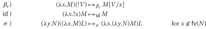
Reduction. The operational semantics of
![]() puts together rules corresponding to the monad laws.
puts together rules corresponding to the monad laws.
Definition 3.3 (Reduction). Relation
![]() is the union of the following rules:
is the union of the following rules:
For every
![]() , reduction
, reduction
![]() is the contextual closure of
is the contextual closure of
![]() , where contexts are defined as follows:
, where contexts are defined as follows:
All reductions in Definition 3.3 are binary relations on
![]() , thanks to the proposition below.
, thanks to the proposition below.
Proposition 3.4. The set of computations
![]() is closed under substitution and reduction:
is closed under substitution and reduction:
(1) If
![]() and
and
![]() , then
, then
![]() .
.
(2) For every
![]() , if
, if
![]() , then:
, then:
![]() if and only if
if and only if
![]() .
.
Proof. Point 1 (formally proved by induction on M) holds because
![]() just replaces a value, x, with another value,
just replaces a value, x, with another value,
![]() . Point 2 is proved by induction on the context for
. Point 2 is proved by induction on the context for
![]() , using Point 1.
, using Point 1.![]()
The computational core
![]() is the rewriting system
is the rewriting system
![]() .
.
Proposition 3.5 (Confluence, de’ Liguoro and Treglia Reference de’ Liguoro and Treglia2020). Reduction
![]() is confluent.
is confluent.
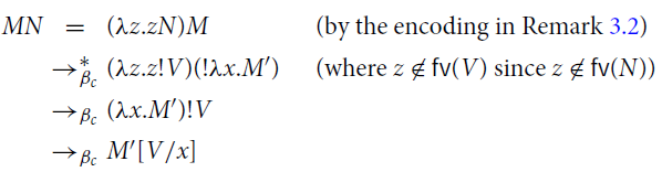
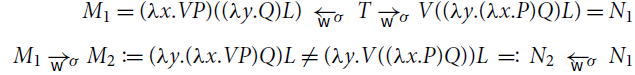
Remark 3.6 (
![]() and
and
![]() ). The relation between
). The relation between
![]() of the computational core and
of the computational core and
![]() of Plotkin’s CbV
of Plotkin’s CbV
![]() -calculus is investigated in Appendix F. To give a taste of it, we show with an example how
-calculus is investigated in Appendix F. To give a taste of it, we show with an example how
![]() -reduction is simulated by
-reduction is simulated by
![]() -reduction, possibly with more steps. Since
-reduction, possibly with more steps. Since
![]() is a relation on
is a relation on
![]() (Proposition 3.4), no computation N will ever reduce to any value V; however, reduction to values is represented by a reduction
(Proposition 3.4), no computation N will ever reduce to any value V; however, reduction to values is represented by a reduction
![]() , where
, where
![]() is the coercion of value V into a computation. Let us assume that
is the coercion of value V into a computation. Let us assume that
![]() and
and
![]() . We have:
. We have:
Similarly, in Plotkin’s CbV
![]() -calculus, if
-calculus, if
![]() and
and
![]() , then
, then
![]() .
.
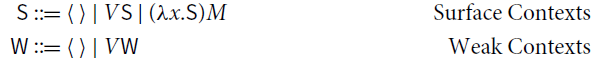
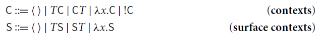
Surface and Weak Reduction. As we shall see in the next sections, there are two natural restrictions of
![]() : weak reduction
: weak reduction
![]() which does not fire in the scope of
which does not fire in the scope of
![]() , and surface reduction
, and surface reduction
![]() , which does not fire in the scope of
, which does not fire in the scope of
![]() . The former is the evaluation usually studied in CbV
. The former is the evaluation usually studied in CbV
![]() -calculus (Theorem 2.11). The latter is the natural evaluation in linear logic, and in Simpson’s calculus, whose relation with
-calculus (Theorem 2.11). The latter is the natural evaluation in linear logic, and in Simpson’s calculus, whose relation with
![]() we discuss in Section 4.
we discuss in Section 4.
Surface and weak contexts are, respectively, defined by the grammars
For
![]() , weak reduction
, weak reduction
![]() is the closure of
is the closure of
![]() under weak contexts
under weak contexts
![]() , surface reduction
, surface reduction
![]() is its closure under surface contexts
is its closure under surface contexts
![]() . non-surface reduction
. non-surface reduction
![]() is the closure of
is the closure of
![]() under contexts
under contexts
![]() that are not surface. Similarly, nonweak reduction
that are not surface. Similarly, nonweak reduction
![]() is the closure of
is the closure of
![]() under contexts
under contexts
![]() that are not weak.
that are not weak.
Clearly,
![]() . Note that
. Note that
![]() is a deterministic relation, while
is a deterministic relation, while
![]() is not.
is not.
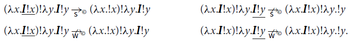
Example 3.7. To clarify the difference between surface and weak, let us consider the term
![]() , where
, where
![]() , and two different
, and two different
![]() steps from it. We underline the fired redex.
steps from it. We underline the fired redex.
Surface reduction can be seen as the natural counterpart of weak reduction in calculi with let-constructors or explicit substitutions, as we show in Section 3.1.
Remark 3.8 (Weak contexts). In the CbV
![]() -calculus (see Section 2.2,), weak contexts can be given in three forms, according to the order in which redexes that are not in the scope of abstractions are fired:
-calculus (see Section 2.2,), weak contexts can be given in three forms, according to the order in which redexes that are not in the scope of abstractions are fired:
![]() . When the grammar of terms is restricted to computations, the three coincide. So, in
. When the grammar of terms is restricted to computations, the three coincide. So, in
![]() there is only one definition of weak context, and weak, left and right reductions coincide.
there is only one definition of weak context, and weak, left and right reductions coincide.
In Sections 4 and 5, we analyze the properties of weak and surface reduction. We first study
![]() , and then we move to the whole
, and then we move to the whole
![]() , where
, where
![]() and
and
![]() also come to play.
also come to play.
Notation. In the rest of the paper, we adopt the following notation:
3.1 The computational core vs. computational calculi with let-notation
It is natural to compare the computational core
![]() with other untyped computational calculi, and wonder if the analysis of the rewriting theory of
with other untyped computational calculi, and wonder if the analysis of the rewriting theory of
![]() we present in this paper applies to them. There is indeed a rich literature on computational calculi refining Moggi’s
we present in this paper applies to them. There is indeed a rich literature on computational calculi refining Moggi’s
![]() (Moggi 1988 Reference Moggi1989, Reference Moggi1991), most of them use the let -constructor. A standard reference is Sabry and Wadler’s
(Moggi 1988 Reference Moggi1989, Reference Moggi1991), most of them use the let -constructor. A standard reference is Sabry and Wadler’s
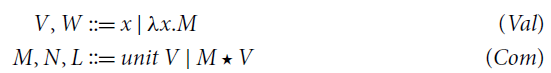
![]() (Sabry and Wadler Reference Sabry and Wadler1997, Section 5), which we display in Figure 1.
(Sabry and Wadler Reference Sabry and Wadler1997, Section 5), which we display in Figure 1.

Figure 1.
![]() : Syntax and reduction.
: Syntax and reduction.
![]() has a two sorted syntax that separates values (i.e., variables and abstractions) and computations. The latter are either let-expressions (aka explicit substitutions, capturing monadic binding), or applications (of values to values), or coercions [V] of values V into computations ([V] is the notation for
has a two sorted syntax that separates values (i.e., variables and abstractions) and computations. The latter are either let-expressions (aka explicit substitutions, capturing monadic binding), or applications (of values to values), or coercions [V] of values V into computations ([V] is the notation for
![]() in Sabry and Wadler (Reference Sabry and Wadler1997), so it corresponds to
in Sabry and Wadler (Reference Sabry and Wadler1997), so it corresponds to
![]() in
in
![]() ).
).
• The reduction rules in
![]() are the usual
are the usual
![]() and
and
![]() from Plotkin’s call-by-value
from Plotkin’s call-by-value
![]() -calculus (Plotkin Reference Plotkin1975), plus the oriented version of three monad laws:
-calculus (Plotkin Reference Plotkin1975), plus the oriented version of three monad laws:
![]() ,
,
![]() ,
,
![]() (see Figure 1).
(see Figure 1).
• Reduction
![]() is the contextual closure of the union of these rules.
is the contextual closure of the union of these rules.
To state a correspondence between
![]() and
and
![]() , consider the translations in Figure 2: translation
, consider the translations in Figure 2: translation
![]() from
from
![]() to
to
![]() (resp.
(resp.
![]() from
from
![]() to
to
![]() ) is defined via the auxiliary encoding
) is defined via the auxiliary encoding
![]() (resp.
(resp.
![]() ) for values. The translations induce an equational correspondence by adding
) for values. The translations induce an equational correspondence by adding
![]() -equality to
-equality to
![]() . More precisely, let
. More precisely, let
![]() be the closure of the rule
be the closure of the rule
![]() (below left) under contexts
(below left) under contexts
![]() (below right).
(below right).
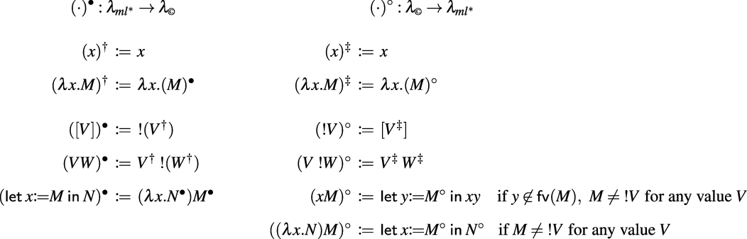
Figure 2. Translations between
![]() and
and
![]() .
.
Let
![]() be the reflexive transitive and symmetric closure of the reduction
be the reflexive transitive and symmetric closure of the reduction
![]() , and similarly for
, and similarly for
![]() with respect to
with respect to
![]() .
.
Proposition 3.9. The following hold:
(1)
![]() for every computation M in
for every computation M in
![]() ;
;
(2)
![]() for every computation P in
for every computation P in
![]() ;
;
(3)
![]() implies
implies
![]() , for every computations M, N in
, for every computations M, N in
![]() ;
;
(4)
![]() implies
implies
![]() , for every computations P, Q in
, for every computations P, Q in
![]() .
.
Proof. (1) By induction on M in
![]() .
.
(2) By induction on P in
![]() .
.
(3) We prove that
![]() implies
implies
![]() , by induction on the definition of
, by induction on the definition of
![]() .
.
(4) We prove that
![]() implies
implies
![]() , by induction on the definition of
, by induction on the definition of
![]() .
.![]()
Proposition 3.9 establishes a precise correspondence between the equational theories of
![]() (including
(including
![]() -conversion) and
-conversion) and
![]() . We had to consider
. We had to consider
![]() since
since
(where
![]() is the reflexive transitive and symmetric closure of
is the reflexive transitive and symmetric closure of
![]() ) and so condition (1) in Proposition 3.9 would not hold if we replace
) and so condition (1) in Proposition 3.9 would not hold if we replace
![]() with
with
![]() .
.
Remark 3.10 (Some intricacies). The correspondence between the reduction theories of
![]() (possibly including
(possibly including
![]() ) and
) and
![]() is not immediate and demands further investigations since, according to the terminology in Sabry and Wadler (1997), there is no Galois connection: Proposition 3.9 where we replace
is not immediate and demands further investigations since, according to the terminology in Sabry and Wadler (1997), there is no Galois connection: Proposition 3.9 where we replace
![]() with
with
![]() , and
, and
![]() with
with
![]() does not hold. More precisely:
does not hold. More precisely:
• the condition corresponding to Point 1, namely
![]() , fails since
, fails since
![]() when
when
![]() for any value V, see (7) above;
for any value V, see (7) above;
• the condition corresponding to Point 3, namely
![]() implies
implies
![]() , fails because
, fails because
![]() but
but
![]() .
.
Surface vs. Weak Reduction. In this paper, we study not only weak but also surface reduction, as the latter has better rewriting properties than the former. Surface reduction in
![]() can be seen as a natural counterpart to Plotkin’s weak reduction in calculi with the let-constructor, such as
can be seen as a natural counterpart to Plotkin’s weak reduction in calculi with the let-constructor, such as
![]() . Intuitively, a term of the form
. Intuitively, a term of the form
![]() can be interpreted as syntactic sugar for
can be interpreted as syntactic sugar for
![]() , however, in the expression
, however, in the expression
![]() , it is not obvious that weak reduction should avoid firing redexes in N. The distinction between
, it is not obvious that weak reduction should avoid firing redexes in N. The distinction between
![]() and let allows for a clean interpretation of weak reduction: it forbids reduction under
and let allows for a clean interpretation of weak reduction: it forbids reduction under
![]() , but not under let, which is compatible with surface reduction in
, but not under let, which is compatible with surface reduction in
![]() .
.
Technically, when we embed
![]() in the computational core via the translation
in the computational core via the translation
![]() in Figure 2, weak reduction
in Figure 2, weak reduction
![]() in
in
![]() (defined as the restriction of
(defined as the restriction of
![]() that does not fire under
that does not fire under
![]() ) corresponds to surface reduction
) corresponds to surface reduction
![]() in
in
![]() : if
: if
![]() then
then
![]() but not necessarily
but not necessarily
![]() . Indeed, consider
. Indeed, consider
![]() in
in
![]() , with
, with
![]() ; then
; then
![]() , which is not a weak step, in
, which is not a weak step, in
![]() .
.
4. The Operational Properties of
Since
![]() -reduction is the engine of any
-reduction is the engine of any
![]() -calculus, we start our analysis of the rewriting theory of
-calculus, we start our analysis of the rewriting theory of
![]() by studying the properties of
by studying the properties of
![]() and its surface restriction
and its surface restriction
![]() . As we show in this section,
. As we show in this section,
![]() and
and
![]() have already been studied in the literature: there is an exact correspondence with Simpson’s calculus (Simpson Reference Simpson and Giesl2005), which stems from Girard’s linear logic (Girard Reference Girard1987). Indeed, the operator
have already been studied in the literature: there is an exact correspondence with Simpson’s calculus (Simpson Reference Simpson and Giesl2005), which stems from Girard’s linear logic (Girard Reference Girard1987). Indeed, the operator
![]() in Simpson (Reference Simpson and Giesl2005) (modeling the bang operator from linear logic) behaves exactly as the the operator
in Simpson (Reference Simpson and Giesl2005) (modeling the bang operator from linear logic) behaves exactly as the the operator
![]() in
in
![]() (modeling
(modeling
![]() in computational calculi). It is easily seen that
in computational calculi). It is easily seen that
![]() , that is,
, that is,
![]() when considering only
when considering only
![]() reduction, is nothing but the restriction of the bang calculus to computations. Thus,
reduction, is nothing but the restriction of the bang calculus to computations. Thus,
![]() has the same operational properties as
has the same operational properties as
![]() . In particular, surface factorization and confluence for
. In particular, surface factorization and confluence for
![]() are inherited from the corresponding properties of
are inherited from the corresponding properties of
![]() in Simpson’s calculus.
in Simpson’s calculus.
The Bang Calculus. We call bang calculus the fragment of Simpson’s linear
![]() -calculus (Simpson Reference Simpson and Giesl2005) without linear abstraction. It has also been studied in Ehrhard and Guerrieri (Reference Ehrhard and Guerrieri2016), Guerrieri and Manzonetto (Reference Guerrieri and Manzonetto2019), Faggian and Guerrieri (Reference Faggian and Guerrieri2021), Guerrieri and Olimpieri (Reference Guerrieri and Olimpieri2021) (with the name bang calculus, which we adopt), and it is closely related to Levy’s Call-by-Push-Value (Levy Reference Levy1999).
-calculus (Simpson Reference Simpson and Giesl2005) without linear abstraction. It has also been studied in Ehrhard and Guerrieri (Reference Ehrhard and Guerrieri2016), Guerrieri and Manzonetto (Reference Guerrieri and Manzonetto2019), Faggian and Guerrieri (Reference Faggian and Guerrieri2021), Guerrieri and Olimpieri (Reference Guerrieri and Olimpieri2021) (with the name bang calculus, which we adopt), and it is closely related to Levy’s Call-by-Push-Value (Levy Reference Levy1999).
We briefly recall the bang calculus
![]() . Terms
. Terms
![]() are defined by
are defined by
Contexts (
![]() ) and surface contexts (
) and surface contexts (
![]() ) are generated by the grammars:
) are generated by the grammars:
The reduction
![]() is the closure under context
is the closure under context
![]() of the rule
of the rule
Surface reduction
![]() is the closure of the rule
is the closure of the rule
![]() under surface contexts
under surface contexts
![]() . non-surface reduction
. non-surface reduction
![]() is the closure of the rule
is the closure of the rule
![]() under contexts
under contexts
![]() that are not surface. Surface reduction factorizes
that are not surface. Surface reduction factorizes
![]() .
.
Theorem 4.1 (Surface factorization Simpson Reference Simpson and Giesl2005). In
![]() :
:
(1) Surface factorization of
![]() :
:
![]() .
.
(2) Bang convergence:
![]() for some term R if and only if
for some term R if and only if
![]() for some term S.
for some term S.
Surface reduction is nondeterministic, but satisfies the diamond property of Fact 2.6.
Theorem 4.2 (Confluence and diamond Simpson Reference Simpson and Giesl2005). In
![]() :
:
• reduction
![]() is confluent;
is confluent;
• reduction
![]() is quasi-diamond (and hence confluent).
is quasi-diamond (and hence confluent).
Restriction to Computations. The restriction of the bang calculus to computations, i.e.,
![]() is exactly the same as the fragment of
is exactly the same as the fragment of
![]() with
with
![]() -rule as unique reduction rule, i.e.
-rule as unique reduction rule, i.e.
![]() .
.
First, observe that the set of computations
![]() defined in Section 3 is a subset of the terms
defined in Section 3 is a subset of the terms
![]() , and moreover it is closed under
, and moreover it is closed under
![]() reduction (exactly as in Proposition 3.4). Second, observe that the restriction of contexts and surface contexts to computations, gives exactly the grammar defined in Section 3. Then
reduction (exactly as in Proposition 3.4). Second, observe that the restriction of contexts and surface contexts to computations, gives exactly the grammar defined in Section 3. Then
![]() and
and
![]() are in fact the same, and for every
are in fact the same, and for every
![]() :
:
•
![]() if and only if
if and only if
![]() .
.
•
![]() if and only if
if and only if
![]() .
.
Hence,
![]() in
in
![]() inherits the operational properties of
inherits the operational properties of
![]() , in particular surface factorization and the quasi-diamond property of
, in particular surface factorization and the quasi-diamond property of
![]() (Theorems 4.1 and 4.2). We will use both extensively.
(Theorems 4.1 and 4.2). We will use both extensively.
Fact 4.3 (Properties of
![]() and of its restriction). In
and of its restriction). In
![]() :
:
• reduction
![]() is nondeterministic and confluent;
is nondeterministic and confluent;
• reduction
![]() is quasi-diamond (and hence confluent);
is quasi-diamond (and hence confluent);
• reduction
![]() satisfies surface factorization:
satisfies surface factorization:
![]() .
.
•
![]() for some value V if and only if
for some value V if and only if
![]() for some value W.
for some value W.
In Sections 6 and 7, we shall generalize and refine the last two points, respectively, to reduction
![]() instead of
instead of
![]() .
.
5. Operational Properties of
, Weak and Surface Reduction
We study evaluation and normalization in
![]() via factorization theorems (Section 6), which are based on both weak and surface reductions. The construction we develop in the next sections demands more work than one may expect. This is due to the fact that the rules induced by the monadic laws of associativity and identity make the analysis of the reduction properties nontrivial. In particular – as anticipated in the introduction – weak reduction does not factorize
via factorization theorems (Section 6), which are based on both weak and surface reductions. The construction we develop in the next sections demands more work than one may expect. This is due to the fact that the rules induced by the monadic laws of associativity and identity make the analysis of the reduction properties nontrivial. In particular – as anticipated in the introduction – weak reduction does not factorize
![]() , and has severe drawbacks, which we explain next. Surface reduction behaves better, but still present difficulties. In the rest of this section, we examine their respective properties.
, and has severe drawbacks, which we explain next. Surface reduction behaves better, but still present difficulties. In the rest of this section, we examine their respective properties.
5.1 Weak reduction: the impact of associativity and identity
Weak (left) reduction (Section 2.2) is one of the most common and studied way to implement evaluation in CbV, and more generally in calculi with effects.
Weak
![]() reduction
reduction
![]() , that is, the closure of
, that is, the closure of
![]() under weak contexts is a deterministic relation. However, when including the rules induced by the monadic equation of associativity and identity, the reduction is nondeterministic, nonconfluent, and normal forms are not unique.
under weak contexts is a deterministic relation. However, when including the rules induced by the monadic equation of associativity and identity, the reduction is nondeterministic, nonconfluent, and normal forms are not unique.
This is somehow surprising, given the prominent role of such a reduction in the literature of calculi with effects. Notice that the issues only come from
![]() and
and
![]() , not from
, not from
![]() . To resume:
. To resume:
(1) Reductions
![]() and
and
![]() are nondeterministic, but are both confluent.
are nondeterministic, but are both confluent.
(2)
![]() are nondeterministic, nonconfluent, and their normal forms are not unique, i.e., adding
are nondeterministic, nonconfluent, and their normal forms are not unique, i.e., adding
![]() , weak reductions lose confluence and uniqueness of normal forms.
, weak reductions lose confluence and uniqueness of normal forms.
Example 5.1 (Non-confluence). An example of the nondeterminism of
![]() is the following:
is the following:
Because of the
![]() rule, weak reductions
rule, weak reductions
![]() and
and
![]() are not confluent and their normal forms are not unique (Point 2 above). Indeed, consider
are not confluent and their normal forms are not unique (Point 2 above). Indeed, consider
![]() where
where
![]() and
and
![]() . Then,
. Then,
where
![]() and
and
![]() are different
are different
![]() -normal forms (clearly,
-normal forms (clearly,
![]() ).
).
Reduction
![]() (like
(like
![]() , Theorem 2.11.1) admits weak factorization (Fact F.2 in Appendix F)
, Theorem 2.11.1) admits weak factorization (Fact F.2 in Appendix F)
This is not the case for
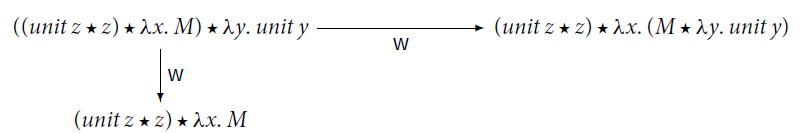
![]() . The following counterexample is due to van Oostrom (Reference van Oostrom2020a).
. The following counterexample is due to van Oostrom (Reference van Oostrom2020a).
Example 5.2 (Nonfactorization van Oostrom Reference van Oostrom2020a). Reduction
![]() does not admit weak factorization. Consider the reduction sequence
does not admit weak factorization. Consider the reduction sequence
M is
![]() -normal and cannot reduce to
-normal and cannot reduce to
![]() by only performing
by only performing
![]() steps (note that
steps (note that
![]() is
is
![]() -normal), hence it is impossible to factorize the sequence from M to
-normal), hence it is impossible to factorize the sequence from M to
![]() as
as
![]() .
.
Let: Different Notation, Same Issues. We stress that the issues are inherent to the associativity and identity rules, not to the specific syntax of
![]() . Exactly the same issues appear in Sabry and Wadler’s
. Exactly the same issues appear in Sabry and Wadler’s
![]() (Sabry and Wadler Reference Sabry and Wadler1997) (see our Figure 1), as we show in the example below.
(Sabry and Wadler Reference Sabry and Wadler1997) (see our Figure 1), as we show in the example below.
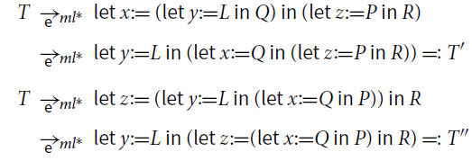
Example 5.3 (Evaluation context in
![]() -notation). In
-notation). In
![]() -notation, the standard evaluation is sequencing (Filinski Reference Filinski1996; Jones et al. Reference Jones, Shields, Launchbury, Tolmach, MacQueen and Cardelli1998; Levy et al. Reference Levy, Power and Thielecke2003), which exactly corresponds to weak reduction in
-notation, the standard evaluation is sequencing (Filinski Reference Filinski1996; Jones et al. Reference Jones, Shields, Launchbury, Tolmach, MacQueen and Cardelli1998; Levy et al. Reference Levy, Power and Thielecke2003), which exactly corresponds to weak reduction in
![]() . The evaluation context for sequencing is
. The evaluation context for sequencing is
We write
![]() for the closure of the
for the closure of the
![]() rules (in Figure 1
) under contexts
rules (in Figure 1
) under contexts
![]() . We observe two problems, the first one due to the rule
. We observe two problems, the first one due to the rule
![]() , the second one to the rule
, the second one to the rule
![]() .
.
(1)
Non-confluence
. Because of the associative rule
![]() , reduction
, reduction
![]() is nondeterministic, nonconfluent, and normal forms are not unique. Consider the following term
is nondeterministic, nonconfluent, and normal forms are not unique. Consider the following term
There are two weak redexes in T, the overlined and the underlined one. Therefore,
where T’ are T” different
![]() -normal forms.
-normal forms.
(2)
Non-factorization
. Because of the
![]() -rule, factorization w.r.t. sequencing does not hold. That is, a reduction sequence
-rule, factorization w.r.t. sequencing does not hold. That is, a reduction sequence
![]() cannot be reorganized as weak steps followed by non-weak steps. Consider the following variation on van Oostrom’s Example 5.2:
cannot be reorganized as weak steps followed by non-weak steps. Consider the following variation on van Oostrom’s Example 5.2:
M is
![]() -normal and cannot reduce to z z by only performing
-normal and cannot reduce to z z by only performing
![]() steps (note that
steps (note that
![]() is
is
![]() -normal), so it is impossible to factorize the sequence form M to zz as
-normal), so it is impossible to factorize the sequence form M to zz as
![]() .
.
5.2 Surface reduction
In
![]() , surface reduction is nondeterministic, but confluent, and well-behaving.
, surface reduction is nondeterministic, but confluent, and well-behaving.
Fact 5.4 (Nondeterminism). For
![]() ,
,
![]() is nondeterministic (because in general more than one surface redex can be fired).
is nondeterministic (because in general more than one surface redex can be fired).
We now analyze confluence of surface reduction. We will use confluence of
![]() (Point 2 below) in Section 8 (Theorem 8.13).
(Point 2 below) in Section 8 (Theorem 8.13).
Proposition 5.5 (Confluence of surface reductions).
(1) Each of the reductions
![]() ,
,
![]() ,
,
![]() is confluent.
is confluent.
(2) Reductions
![]() and
and
![]() are confluent.
are confluent.
(3) Reduction
![]() is confluent.
is confluent.
(4) Reduction
![]() is not confluent.
is not confluent.
Proof. We rely on confluence of
![]() (by Theorem 4.2), and on Hindley–Rosen Lemma (Lemma 2.9). We prove commutation via strong commutation (Lemma 2.10). The only delicate point is the commutation of
(by Theorem 4.2), and on Hindley–Rosen Lemma (Lemma 2.9). We prove commutation via strong commutation (Lemma 2.10). The only delicate point is the commutation of
![]() with
with
![]() (Points 3 and 4).
(Points 3 and 4).
(1)
![]() is locally confluent and terminating, and so confluent;
is locally confluent and terminating, and so confluent;
![]() is quasi-diamond (in the sense of Fact 2.6), and hence also confluent.
is quasi-diamond (in the sense of Fact 2.6), and hence also confluent.
(2) It is easily verified that
![]() and
and
![]() strongly commute and similarly for
strongly commute and similarly for
![]() and
and
![]() . The claim then follows by Hindley–Rosen Lemma.
. The claim then follows by Hindley–Rosen Lemma.
(3)
![]() strongly commutes with
strongly commutes with
![]() . This point is delicate because to close a diagram of the shape
. This point is delicate because to close a diagram of the shape
![]() may require a
may require a
![]() step, see Example 5.7. The claim then follows by Hindley–Rosen Lemma.
step, see Example 5.7. The claim then follows by Hindley–Rosen Lemma.
(4) A counterexample is provided by the same diagram mentioned in the previous point (Example 5.7), requiring a
![]() step to close.
step to close.![]()
Example 5.6. Let us give an example for nondeterminism and confluence of surface reduction.
(1) Non-determinism: Consider the term
![]() where R and R’ are any redexes.
where R and R’ are any redexes.
(2) Confluence: Consider the same term as in Example 5.1:
![]() . Then,
. Then,
Now we can close the diagram:
Example 5.7. In the following counterexample to confluence of
![]() , where
, where
![]() , the
, the
![]() -redex overlaps with the
-redex overlaps with the
![]() -redex. The corresponding steps are surface (and even weak) and the only way to close the diagram is by means of a
-redex. The corresponding steps are surface (and even weak) and the only way to close the diagram is by means of a
![]() step, which is also surface (but not weak).
step, which is also surface (but not weak).
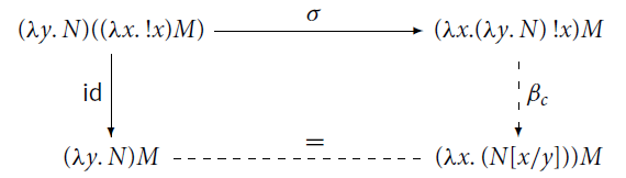
Note that
![]() , and so
, and so
![]() , since
, since
![]() is the term obtained from
is the term obtained from
![]() by renaming its bound variable y to x.
by renaming its bound variable y to x.
This is also a counterexample to confluence of
![]() and of
and of
![]() .
.
In Section 6, we prove that surface reduction does factorize
![]() , similarly to what happens for Simpson’s calculus (Theorem 4.1). Surface reduction also has a drawback: it does not allows us to separate
, similarly to what happens for Simpson’s calculus (Theorem 4.1). Surface reduction also has a drawback: it does not allows us to separate
![]() and
and
![]() steps. This fact makes it difficult to reason about returning a value.
steps. This fact makes it difficult to reason about returning a value.
Example 5.8 (An issue with surface reduction). Consider the term
![]() , which is normal for
, which is normal for
![]() and in particular for
and in particular for
![]() , but
, but
Here it is not possible to postpone a step
![]() after a step
after a step
![]() .
.
5.3 Confluence properties of
,
and
Finally, we briefly revisit the confluence of
![]() , already established in de' Liguoro and Treglia (2020), in order to analyze the confluence properties of the different subsystems too. This completes the analysis given in Proposition 5.5. In Section 8, we will use confluence of
, already established in de' Liguoro and Treglia (2020), in order to analyze the confluence properties of the different subsystems too. This completes the analysis given in Proposition 5.5. In Section 8, we will use confluence of
![]() (Theorem 8.14).
(Theorem 8.14).
Proposition 5.9 (Confluence of
![]() ,
,
![]() and
and
![]() ).
).
(1) Each of the reductions
![]() ,
,
![]() ,
,
![]() is confluent.
is confluent.
(2) Reductions
![]() and
and
![]() are confluent.
are confluent.
(3) Reduction
![]() is confluent.
is confluent.
(4) Reduction
![]() is not confluent.
is not confluent.
Proof. We rely on confluence of
![]() (by Theorem 4.2), and on Hindley–Rosen Lemma (Lemma 2.9). We prove commutation via strong commutation (Lemma 2.10). The only delicate point is again the commutation of
(by Theorem 4.2), and on Hindley–Rosen Lemma (Lemma 2.9). We prove commutation via strong commutation (Lemma 2.10). The only delicate point is again the commutation of
![]() with
with
![]() (Points 3 and 4).
(Points 3 and 4).
(1)
![]() is locally confluent and terminating, and so confluent.
is locally confluent and terminating, and so confluent.
![]() is quasi-diamond in the sense of Fact 2.6, and hence confluent.
is quasi-diamond in the sense of Fact 2.6, and hence confluent.
(2) It is easily verified that
![]() and
and
![]() strongly commute, and
strongly commute, and
![]() and
and
![]() do as well. The claim then follows by Hindley–Rosen Lemma.
do as well. The claim then follows by Hindley–Rosen Lemma.
(3)
![]() strongly commutes with
strongly commutes with
![]() . This point is delicate because to close a diagram of the shape
. This point is delicate because to close a diagram of the shape
![]() may require a
may require a
![]() step (see Example 5.7). The claim then follows by Hindley–Rosen Lemma.
step (see Example 5.7). The claim then follows by Hindley–Rosen Lemma.
(4) A counterexample is provided by the same diagram mentioned in the previous point (Example 5.7), requiring a
![]() step to close.
step to close.![]()
6. Surface and Weak Factorization
In this section, we prove several factorization results for
![]() . Surface factorization is the cornerstone for the subsequent development. It is proved in Section 6.1.
. Surface factorization is the cornerstone for the subsequent development. It is proved in Section 6.1.
Theorem 6.1. [Surface factorization in
![]() ] Reduction
] Reduction
![]() admits surface factorization:
admits surface factorization:
We then refine this result first by postponing
![]() steps that are not also
steps that are not also
![]() steps, and then by means of weak factorization (on surface steps). This further phases serve two purposes:
steps, and then by means of weak factorization (on surface steps). This further phases serve two purposes:
(1) to postpone non-weak
![]() steps after weak
steps after weak
![]() steps, and
steps, and
(2) to separate weak
![]() and
and
![]() steps, by postponing
steps, by postponing
![]() steps after
steps after
![]() steps, and
steps, and
(3) to perform a fine analysis of quantitative properties, namely the number of
![]() steps.
steps.
We will need Points 1 and 2 to define evaluation relations (Section 7) and Point 3 to define normalizing strategies (Section 8).
Technical Lemmas. We shall often exploit some basic properties of contextual closure, which we collect here. In any variant of the
![]() -calculus, if a step
-calculus, if a step
![]() is obtained by the closure of a rule
is obtained by the closure of a rule
![]() under a non-empty context (i.e., a context other than the hole), then T and T’ have the same shape, that is, they are both applications or both abstractions or both variables or both !-terms.
under a non-empty context (i.e., a context other than the hole), then T and T’ have the same shape, that is, they are both applications or both abstractions or both variables or both !-terms.
Fact 6.2 (Shape preservation) Let
![]() be a rule and
be a rule and
![]() be its contextual closure. Assume
be its contextual closure. Assume
![]() where
where
![]() and
and
![]() . Then T and T’ have the same shape.
. Then T and T’ have the same shape.
An easy-to-verify consequence of Fact 6.2 in
![]() is the following.
is the following.
Lemma 6.3 (Redexes preservation). Let
![]() and
and
![]() : M is a
: M is a
![]() -redex if and only if N is a
-redex if and only if N is a
![]() -redex.
-redex.
Proof. See the Appendix, namely Corollary B.2 for
![]() , and Lemma C.1 for
, and Lemma C.1 for
![]() .
.![]()
Lemma 6.3 is false if we replace the hypothesis
![]() with
with
![]() . Indeed, consider
. Indeed, consider
![]() : N is a
: N is a
![]() -redex but M is not.
-redex but M is not.
Notice the following inclusions, which we will use freely.
Fact 6.4.
![]() and
and
![]() , because a weak context is necessarily a surface context (but a surface context need not be a weak context, e.g. the surface context
, because a weak context is necessarily a surface context (but a surface context need not be a weak context, e.g. the surface context
![]() is not weak).
is not weak).
6.1 Surface factorizations in
, modularly
We prove surface factorization in
![]() . We already know that surface factorization holds for
. We already know that surface factorization holds for
![]() (Fact 4.3), so we can rely on it, and work modularly, following the approach proposed in Accattoli et al. (Reference Accattoli, Faggian and Guerrieri2021). The tests for call-by-name head factorization and call-by-value weak factorization in Accattoli et al. (Reference Accattoli, Faggian and Guerrieri2021) easily adapt to surface factorization in
(Fact 4.3), so we can rely on it, and work modularly, following the approach proposed in Accattoli et al. (Reference Accattoli, Faggian and Guerrieri2021). The tests for call-by-name head factorization and call-by-value weak factorization in Accattoli et al. (Reference Accattoli, Faggian and Guerrieri2021) easily adapt to surface factorization in
![]() , yielding the following convenient test. It modularly establishes surface factorization of a reduction
, yielding the following convenient test. It modularly establishes surface factorization of a reduction
![]() , where
, where
![]() is a new reduction added to
is a new reduction added to
![]() . Details of the proof are in Appendices B.2 and B.3.
. Details of the proof are in Appendices B.2 and B.3.
Proposition 6.5 (A modular test for surface factorization with
![]() ) Let
) Let
![]() be the contextual closure of a rule
be the contextual closure of a rule
![]() . Reduction
. Reduction
![]() satisfies surface factorization (that is,
satisfies surface factorization (that is,
![]() ) if:
) if:
(1) Surface factorization of
![]() :
:
![]() .
.
(2)
![]() is substitutive:
is substitutive:
![]()
(3) Root linear swap:
![]() .
.
We will use the following easy property (an instance of Lemma B.4 in the Appendix).
Lemma 6.6. Let
![]() be the contextual closure of rules
be the contextual closure of rules
![]() . Then,
. Then,
![]() implies
implies
![]() .
.
Root Lemmas. Lemmas 6.7 and 6.8 below provide everything we need to verify the conditions of the modular test in Proposition 6.5, and so to establish surface factorization in
![]() .
.
Lemma 6.7 (
![]() -Roots). Let
-Roots). Let
![]() . The following holds:
. The following holds:
Proof. We have
![]() . Since L is a
. Since L is a
![]() -redex, M also is a
-redex, M also is a
![]() -redex (Lemma 6.3). So
-redex (Lemma 6.3). So
![]() , where for only one
, where for only one
![]()
![]() and otherwise
and otherwise
![]() , for
, for
![]() (by Fact B.1 in the Appendix). Therefore,
(by Fact B.1 in the Appendix). Therefore,
![]() .
.![]()
Lemma 6.8 (
![]() -Roots). Let
-Roots). Let
![]() . The following holds:
. The following holds:
Proof. We have
![]() . Since L is an
. Since L is an
![]() -redex, M also is (Lemma 6.3). So,
-redex, M also is (Lemma 6.3). So,
![]() for some
for some
![]() . Therefore,
. Therefore,
![]() .
.![]()
Let us make explicit the content of the two lemmas above. By instantiating
![]() in Lemmas 6.7 and 6.8, and combining them with Lemma 6.6, we obtain the following facts:
in Lemmas 6.7 and 6.8, and combining them with Lemma 6.6, we obtain the following facts:
Fact 6.9.
![]() implies
implies
![]() and so (Lemma 6.6)
and so (Lemma 6.6)
![]() implies
implies
![]() ( i.e. strong postponement holds).
( i.e. strong postponement holds).
(2)
![]() implies
implies
![]() and so (Lemma 6.6)
and so (Lemma 6.6)
![]() implies
implies
![]() .
.
(3)
![]() implies
implies
![]() .
.
Fact 6.10. (1)
![]() implies
implies
![]() , and so (Lemma 6.6)
, and so (Lemma 6.6)
![]() implies
implies
![]() ( i.e. strong postponement holds).
( i.e. strong postponement holds).
(2)
![]() implies
implies
![]() , and so (Lemma 6.6)
, and so (Lemma 6.6)
![]() implies
implies
![]() .
.
(3)
![]() implies
implies
![]() .
.
Surface Factorization of
![]() . We can now combine the facts above concerning
. We can now combine the facts above concerning
![]() and
and
![]() steps, using the modular approach proposed in Accattoli et al. (Reference Accattoli, Faggian and Guerrieri2021) (see Theorem B.3 in the Appendix), to prove surface factorization of
steps, using the modular approach proposed in Accattoli et al. (Reference Accattoli, Faggian and Guerrieri2021) (see Theorem B.3 in the Appendix), to prove surface factorization of
![]() .
.
Lemma 6.11 (Surface factorization of
![]() ) Surface factorization of
) Surface factorization of
![]() holds, because:
holds, because:
(1) Surface factorization of
![]() holds (that is,
holds (that is,
![]() ).
).
(2) Surface factorization of
![]() holds (that is,
holds (that is,
![]() ).
).
(3) Linear swap:
![]() .
.
(4) Linear swap:
![]() .
.
Proof. Points 1 and 2 follow from Fact 6.9.1 and Fact 6.10.1, respectively, by (linear) strong postponement (Lemma 2.5). Point 3 is Fact 6.9.2. Point 4 is Fact 6.10.2.![]()
Surface Factorization of
![]() , Modularly. We are now ready to use the modular test for surface factorization with
, Modularly. We are now ready to use the modular test for surface factorization with
![]() (Proposition 6.5) to prove Theorem 6.1.
(Proposition 6.5) to prove Theorem 6.1.
Theorem 6.1. [Surface factorization in
![]() ] Reduction
] Reduction
![]() admits surface factorization:
admits surface factorization:
Proof. All conditions in Proposition 6.5 hold, namely
(1) Surface factorization of
![]() holds by Lemma 6.11.
holds by Lemma 6.11.
(2) Substitutivity:
![]() and
and
![]() are substitutive (the proof is immediate).
are substitutive (the proof is immediate).
(3) Root linear swap: for
![]() ,
,
![]() by Fact 6.9.3 and Fact 6.10.3.
by Fact 6.9.3 and Fact 6.10.3.![]()
Interestingly, the same machinery can also be used to prove another surface factorization result, which says that surface factorization, when applied to
![]() only, does not create
only, does not create
![]() steps.
steps.
Proposition 6.12 (Surface factorization of
![]() ). Reduction
). Reduction
![]() admits surface factorization:
admits surface factorization:
Proof. All conditions in Proposition 6.5 hold, namely
(1) Surface factorization of
![]() holds by Fact 6.9.1 and strong postponement (Lemma 2.5).
holds by Fact 6.9.1 and strong postponement (Lemma 2.5).
(2) Substitutivity:
![]() is substitutive (the proof is immediate).
is substitutive (the proof is immediate).
(3) Root linear swap:
![]() by Fact 6.9.3.
by Fact 6.9.3.![]()
The fact that two similar factorization results (Theorem 6.1 and Proposition 6.12) can be proven by means of the same modular test (Proposition 6.5) fed on similar lemmas shows one of the benefits of our modular approach: passing from one result to the other is smooth and effortless.
6.2 A closer look at
steps, via postponement
We show a postponement result for
![]() steps on which evaluation (Section 7) and normalization (Section 8) rely. Note that
steps on which evaluation (Section 7) and normalization (Section 8) rely. Note that
![]() overlaps with
overlaps with
![]() . We define
. We define
![]() as a
as a
![]() step that is not
step that is not
![]() .
.
Clearly,
![]() . In the proofs, it is convenient to split
. In the proofs, it is convenient to split
![]() into steps that are also
into steps that are also
![]() steps, and those that are not.
steps, and those that are not.
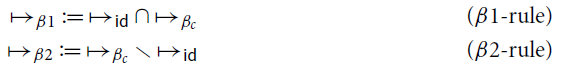
Notice that
![]() .
.
We prove that
![]() steps can be postponed after both
steps can be postponed after both
![]() and
and
![]() steps, by using van Oostrom’s decreasing diagrams technique (van Oostrom Reference van Oostrom1994, Reference van Oostrom2008) (Theorem 2.8). The proof closely follows van Oostrom’s proof of the postponement of
steps, by using van Oostrom’s decreasing diagrams technique (van Oostrom Reference van Oostrom1994, Reference van Oostrom2008) (Theorem 2.8). The proof closely follows van Oostrom’s proof of the postponement of
![]() after β (Reference van Oostromvan Oostrom 2020b).
after β (Reference van Oostromvan Oostrom 2020b).
Theorem 6.13 (Postponement of
![]() ). If
). If
![]() , then
, then
![]() .
.
Proof. Let
![]() and let
and let
![]() . We equip the labels
. We equip the labels
![]() with the following (well-founded) order
with the following (well-founded) order
We prove that the pair of relations
![]() is decreasing by checking the following three local commutations hold (the technical details are in the Appendix):
is decreasing by checking the following three local commutations hold (the technical details are in the Appendix):
(1)
![]() (see Lemma C.3);
(see Lemma C.3);
(2)
![]() (see Lemma C.4);
(see Lemma C.4);
(3)
![]() (see Lemma C.5).
(see Lemma C.5).
Hence, by Theorem 2.8, the relations
![]() and
and
![]() commute. That is,
commute. That is,
![]() postpones after
postpones after
![]() :
:
Or equivalently (Lemma 2.4),
![]() .
.![]()
Corollary 6.14 (Surface factorization
![]() postponement). If
postponement). If
![]() , then
, then
![]() .
.
Proof. Immediate consequence of
![]() -postponement (Theorem 6.13) and of surface factorization of the resulting initial
-postponement (Theorem 6.13) and of surface factorization of the resulting initial
![]() -sequence (Proposition 6.12).
-sequence (Proposition 6.12).![]()
6.3 Weak factorization
Thanks to surface factorization plus
![]() -postponement (Corollary 6.14), every
-postponement (Corollary 6.14), every
![]() -sequence can be rearranged so that it starts with an
-sequence can be rearranged so that it starts with an
![]() -sequence. We show now that such an initial
-sequence. We show now that such an initial
![]() -sequence can in turn be factorized into weak steps followed by non-weak steps. This weak factorization result will be used in Section 7 to obtain evaluation via weak
-sequence can in turn be factorized into weak steps followed by non-weak steps. This weak factorization result will be used in Section 7 to obtain evaluation via weak
![]() steps (Theorem 7.6).
steps (Theorem 7.6).
Remarkably, weak factorization of an
![]() -sequence preserves the number of
-sequence preserves the number of
![]() steps. This property has no role with respect to evaluation, but it will be crucial when we investigate normalizing strategies in Section 8. For this reason, we include it in the statement of Theorem 6.16.
steps. This property has no role with respect to evaluation, but it will be crucial when we investigate normalizing strategies in Section 8. For this reason, we include it in the statement of Theorem 6.16.
Quantitative Linear Postponement. Let us take an abstract point of view. The condition in Lemma 2.5 – Hindley’s strong postponement – can be refined into quantitative (linear) variants, which allow us to “count the steps” and are useful to establish termination properties.
Lemma 6.15 (Linear postponement). Let
![]() be an ARS with
be an ARS with
![]() .
.
• If
![]() , then
, then
![]() implies
implies
![]() and the two sequences have the same number of
and the two sequences have the same number of
![]() steps.
steps.
• For all
![]() with L a set of indices, let
with L a set of indices, let
![]() and
and
 and
and
 . Assume
Then,
![]() implies
implies
![]() and the two sequences have the same number of
and the two sequences have the same number of
![]() steps, for each
steps, for each
![]() .
.
Observe that in (8), the last step is
![]() , not necessarily
, not necessarily
![]() .
.
Weak Factorization. We show two kinds of weak factorization: a surface
![]() sequence can be reorganized, so that non-weak
sequence can be reorganized, so that non-weak
![]() steps are postponed after the weak ones; and a weak
steps are postponed after the weak ones; and a weak
![]() sequence can in turn be rearranged so that weak
sequence can in turn be rearranged so that weak
![]() steps are before weak
steps are before weak
![]() steps.
steps.
Theorem 6.16 (Weak factorization).
(1) If
![]() then
then
![]() where all steps are surface, and the two sequences have the same number of
where all steps are surface, and the two sequences have the same number of
![]() steps.
steps.
(2) If
![]() then
then
![]() , and the two sequences have the same number of
, and the two sequences have the same number of
![]() steps.
steps.
Proof. In both claims, we use Lemma 6.15. Its linearity allows us to count the
![]() steps. In the proof, we write
steps. In the proof, we write
![]() (resp.
(resp.
![]() ) for
) for
![]() (resp.
(resp.
![]() ).
).
(1) Let
![]() (i.e.,
(i.e.,
![]() is a surface step whose redex is in the scope of a
is a surface step whose redex is in the scope of a
![]() ). We prove linear postponement:
). We prove linear postponement:
Assume
![]() : M and L have the same shape, which is not
: M and L have the same shape, which is not
![]() , otherwise no weak or surface step from M is possible. We examine the cases.
, otherwise no weak or surface step from M is possible. We examine the cases.
- The step
![]() has empty context:
has empty context:
-
![]() Then,
Then,
![]() , and
, and
![]() with
with
![]() . Therefore,
. Therefore,
![]() .
.
-
![]() . Then,
. Then,
![]() , and
, and
![]() where exactly one among
where exactly one among
![]() reduces to V, P, Q, respectively, the other two are unchanged. So,
reduces to V, P, Q, respectively, the other two are unchanged. So,
![]() .
.
- The step
![]() has nonempty context. Necessarily, we have
has nonempty context. Necessarily, we have
![]() , with
, with
![]() :
:
- Case
![]() with
with
![]() and
and
![]() , then
, then
![]() .
.
- Case
![]() with
with
![]() . We conclude by i.h. .
. We conclude by i.h. .
Observe that we have proved more than (9), namely we proved
So, we conclude that the two sequences have the same number of
![]() steps, by Lemma 6.15.
steps, by Lemma 6.15.
(2) We prove
![]() similarly to Point 1 and conclude by Lemma 6.15.
similarly to Point 1 and conclude by Lemma 6.15.![]()
Combining Points 1 and 2 in Theorem 6.16, we deduce that
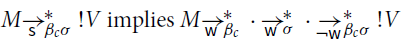
and the two sequences from M to
![]() have the same number of
have the same number of
![]() steps.
steps.
7. Returning a Value
In this section, we focus on values. They are the terms of interest in the CbV
![]() -calculus. Also, for weak reduction there, closed values are exactly the normal forms of closed terms, i.e., of programs.
-calculus. Also, for weak reduction there, closed values are exactly the normal forms of closed terms, i.e., of programs.
In a computational setting such as
![]() , we are interested in knowing if a term M returns a value, i.e. if
, we are interested in knowing if a term M returns a value, i.e. if
![]() for some value V, noted
for some value V, noted
![]() (the computation
(the computation
![]() is sometimes called a returned value, in that it is the coercion of a value V to the computational level). Since a term may be reduced in several ways and so its reduction graph can become quite complicated, it is natural to search for deterministic reductions to return a value. Hence, the question is if M returns a value, is there a deterministic reduction (called evaluation) from M that is guaranteed to return a value? The answer is positive. In fact, there are two such reductions:
is sometimes called a returned value, in that it is the coercion of a value V to the computational level). Since a term may be reduced in several ways and so its reduction graph can become quite complicated, it is natural to search for deterministic reductions to return a value. Hence, the question is if M returns a value, is there a deterministic reduction (called evaluation) from M that is guaranteed to return a value? The answer is positive. In fact, there are two such reductions:
![]() and
and
![]() (Theorem 7.4 below).
(Theorem 7.4 below).
Recall that
![]() is the union of two rules without any contextual closure. Thanks to their simple reduction graph, deterministic reductions are quite useful in particular for proving negative results such as showing that a computation cannot return a value.
is the union of two rules without any contextual closure. Thanks to their simple reduction graph, deterministic reductions are quite useful in particular for proving negative results such as showing that a computation cannot return a value.
Fact 7.1. In
![]() , reductions
, reductions
![]() ,
,
![]() ,
,
![]() , and
, and
![]() are deterministic.
are deterministic.
In
![]() one of the reasons for the interest in values is that, akin to the CbV
one of the reasons for the interest in values is that, akin to the CbV
![]() -calculus, closed ( i.e. , without free variables) returned values are exactly the closed normal forms for weak reductions
-calculus, closed ( i.e. , without free variables) returned values are exactly the closed normal forms for weak reductions
![]() and
and
![]() . This is a consequence of the following syntactic characterizations of normal forms.
. This is a consequence of the following syntactic characterizations of normal forms.
Proposition 7.2.
A computation is normal for reduction
![]() (resp.
(resp.
![]() ;
;
![]() ) if and only if it is of the form
) if and only if it is of the form
![]() (resp.
(resp.
![]() ;
;
![]() ) defined below, where
) defined below, where
![]() denotes a computation
denotes a computation
![]() for any
for any
![]() .
.
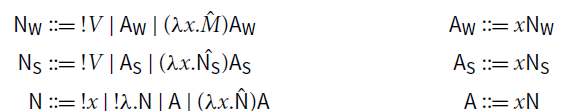
Proof. The right-to-left part is proved by induction on
![]() (resp.
(resp.
![]() ;
;
![]() ). The left-to-right part follows easily from the observation that every computation can be written in a unique way as
). The left-to-right part follows easily from the observation that every computation can be written in a unique way as
![]() for some
for some
![]() and some values
and some values
![]() .
.![]()
Corollary 7.3 (Closed normal forms). Let
![]() . A closed computation is
. A closed computation is
![]() -normal if and only if it is a returned value.
-normal if and only if it is a returned value.
Proof. Computations of shape
![]() and
and
![]() have a free variable. So, according to Proposition 7.2, closed returned values are all and only the closed normal forms for
have a free variable. So, according to Proposition 7.2, closed returned values are all and only the closed normal forms for
![]() and
and
![]() .
.
Moreover, since every closed computation M can be written in a unique way as
![]() for some
for some
![]() and some closed values
and some closed values
![]() , if M is
, if M is
![]() -normal or
-normal or
![]() -normal then
-normal then
![]() (otherwise
(otherwise
![]() would be a
would be a
![]() -redex), hence M is a returned value.
-redex), hence M is a returned value.![]()
Corollary 7.3 means that reductions
![]() behave differently only on open computations (that is, with at least one free variable).
behave differently only on open computations (that is, with at least one free variable).
We can now state the main result in this section. Sections 7.1 and 7.2 are devoted to prove it.
Theorem 7.4 (Returning a value). The following are equivalent:
(1) M returns a value, i.e.
![]() .
.
(2) The maximal
![]() -sequence from M is finite and ends in a returned value
-sequence from M is finite and ends in a returned value
![]() .
.
(3) The maximal
![]() -sequence from M is finite and ends in a returned value
-sequence from M is finite and ends in a returned value
![]() .
.
Proof.
![]() is Theorem7.6 below, which we prove in forthcoming Section 7.1.
is Theorem7.6 below, which we prove in forthcoming Section 7.1.
![]() is Proposition 7.10 below, which we prove in forthcoming Section 7.2.
is Proposition 7.10 below, which we prove in forthcoming Section 7.2.
![]() is trivial.
is trivial.
Note that Theorem 7.4 (and hence the analysis that will follow) is not restricted to closed terms. Indeed, an open term may well return a value. For example,
![]() or
or
![]() or
or
![]() .
.
7.1 Values via weak
steps
Thanks to factorization, we can prove that
![]() steps suffice to return a value. This is an immediate consequence of surface factorization plus
steps suffice to return a value. This is an immediate consequence of surface factorization plus
![]() postponement (Corollary 6.14), and weak factorization (Theorem 6.16), and the fact that non-weak steps,
postponement (Corollary 6.14), and weak factorization (Theorem 6.16), and the fact that non-weak steps,
![]() steps, and
steps, and
![]() steps cannot produce
steps cannot produce
![]() -terms.
-terms.
Lemma 7.5.
If
![]() with a step that is not
with a step that is not
![]() , then
, then
![]() for some value W.
for some value W.
Proof. Indeed, one can easily check the following (recall that
![]() ).
).
• If
![]() , then
, then
![]() for some value W (proof by induction on M).
for some value W (proof by induction on M).
• If
![]() , then
, then
![]() for some value W (proof by induction on M).
for some value W (proof by induction on M).
• If
![]() , then
, then
![]() for some value W (by shape preservation, Fact 6.2).
for some value W (by shape preservation, Fact 6.2).![]()
Theorem 7.6 (Values via weak
![]() steps). The following are equivalent:
steps). The following are equivalent:
(1)
![]() for some
for some
![]() ;
;
(2)
![]() for some
for some
![]() .
.
Proof. Point 2 trivially implies Point 1, as
![]() . Let us show that Point 1 entails Point 2.
. Let us show that Point 1 entails Point 2.
If
![]() then
then
![]() by surface factorization plus
by surface factorization plus
![]() postponement (Corollary 6.14). By weak factorization (Theorem 6.16.1-2), we have
postponement (Corollary 6.14). By weak factorization (Theorem 6.16.1-2), we have
By iterating Lemma 7.5 from
![]() backward (and since
backward (and since
![]() ), we have that all terms in the sequence from M’ to
), we have that all terms in the sequence from M’ to
![]() are
are
![]() -terms. So in particular, M’ has shape
-terms. So in particular, M’ has shape
![]() for some value W.
for some value W.![]()
Remark 7.7. Theorem 7.6 was already claimed in de' Liguoro and Treglia (2020), for closed terms. However, the inductive argument there (which does not use any factorization) is fallacious, it does not suffice to produce a complete proof in the case where
![]() .
.
7.2 Values via
root steps
We also show an alternative way to evaluate a term in
![]() . Let us call root steps the rules
. Let us call root steps the rules
![]() and
and
![]() . The first two suffice to return a value, without the need for any contextual closure.
. The first two suffice to return a value, without the need for any contextual closure.
Note that this property holds only because terms are restricted to computations (for example, in Plotkin’s CbV
![]() -calculus, (II)(II) can be reduced, but it is not itself a redex, so
-calculus, (II)(II) can be reduced, but it is not itself a redex, so
![]() ).
).
Looking closer at the proof of Corollary 7.3, we observe that any closed ( i.e. without free variables) computation has the following property: it is either a returned value (when
![]() ), or a
), or a
![]() -redex (when
-redex (when
![]() ) or a
) or a
![]() -redex (when
-redex (when
![]() ). More generally, the same holds for any (possibly open) computation that returns a value (Corollary 7.9 below).
). More generally, the same holds for any (possibly open) computation that returns a value (Corollary 7.9 below).
Lemma 7.8. Assume
![]() for some value W. Then,
for some value W. Then,
• either
![]() ,
,
• or
![]() and
and
![]() , for some value U.
, for some value U.
Thus,
![]() , where
, where
![]() and the
and the
![]() ’s are abstractions, and if
’s are abstractions, and if
![]() then
then
![]() .
.
Corollary 7.9 (Progression via root steps). If M returns a value ( i.e.
![]() for some value W), then M is either a
for some value W), then M is either a
![]() -redex, or a
-redex, or a
![]() -redex, or it has shape
-redex, or it has shape
![]() for some value V.
for some value V.
Proof. By Theorem 7.6,
![]() for some value W’. By Lemma 7.8, we conclude.
for some value W’. By Lemma 7.8, we conclude.![]()
Corollary 7.9 states a progression results: a
![]() -sequence from M may only end in a
-sequence from M may only end in a
![]() -term. We still need to verify that such a sequence terminates.
-term. We still need to verify that such a sequence terminates.
Proposition 7.10 (Weak steps and root steps). If
![]() then
then
![]() . Moreover, the two sequences have the same number of
. Moreover, the two sequences have the same number of
![]() steps.
steps.
Proof. By induction on the number k of
![]() steps. If
steps. If
![]() the claim holds trivially. Otherwise,
the claim holds trivially. Otherwise,
![]() and by i.h.
and by i.h.
• If M is
![]() -redex, then
-redex, then
![]() by determinism of
by determinism of
![]() (Fact 7.1), and the claim is proved.
(Fact 7.1), and the claim is proved.
• If M is a
![]() -redex, observe that by Lemma 7.8,
-redex, observe that by Lemma 7.8,
-
![]() , and
, and
-
![]() .
.
We apply all possible
![]() steps starting from M, obtaining
steps starting from M, obtaining
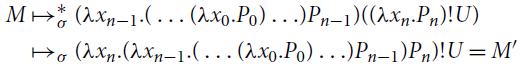
which is a
![]() -redex, so
-redex, so
![]() (note that we used the hypothesis on free variables of
(note that we used the hypothesis on free variables of
![]() ). We observe that
). We observe that
![]() . We conclude, by using (10) and the fact that
. We conclude, by using (10) and the fact that
![]() is deterministic (Fact 7.1).
is deterministic (Fact 7.1).![]()
The converse of Proposition 7.10 is also true and immediate. We can finally prove that root steps
![]() and
and
![]() suffice to return a value, without the need for any contextual closure.
suffice to return a value, without the need for any contextual closure.
Theorem 7.11 (Values via root
![]() steps). The following are equivalent:
steps). The following are equivalent:
(1)
![]() for some
for some
![]() ;
;
(2)
![]() for some
for some
![]() .
.
Proof. Trivially (2)
![]() (1). Conversely, (1)
(1). Conversely, (1)
![]() (2) Proposition 7.10 and Theorem 7.6.
(2) Proposition 7.10 and Theorem 7.6.![]()
7.3 Observational equivalence
We now adapt the notion of observational equivalence, introduced in Plotkin (Reference Plotkin1975) for the CbV
![]() -calculus, to
-calculus, to
![]() . Informally, two terms are observationally equivalent if they can be substituted for each other in all contexts without observing any difference in their behavior. For a computation M in
. Informally, two terms are observationally equivalent if they can be substituted for each other in all contexts without observing any difference in their behavior. For a computation M in
![]() , the “behavior” of interest is returning a value:
, the “behavior” of interest is returning a value:
![]() for some value V, also noted
for some value V, also noted
![]() .
.
Definition 7.12 (Observational equivalence). Let
![]() . We say that M and N are observationally equivalent, noted
. We say that M and N are observationally equivalent, noted
![]() , if for every context
, if for every context
![]() if and only if
if and only if
![]() .
.
A consequence of Theorem 7.6 is that the behavior of interest in Definition 7.12 can be equivalently defined as
![]() for some value V, instead of
for some value V, instead of
![]() : the resulting notion of observational equivalence would be exactly the same. The definition using
: the resulting notion of observational equivalence would be exactly the same. The definition using
![]() instead of
instead of
![]() is more in the spirit of Plotkin’s original one for the CbV
is more in the spirit of Plotkin’s original one for the CbV
![]() -calculus (Plotkin Reference Plotkin1975). Reduction
-calculus (Plotkin Reference Plotkin1975). Reduction
![]() is deterministic, and for closed terms it terminates if and only if it ends in a returned value (Corollary 7.3). Hence, for closed terms, returning a value amounts to say that their evaluation
is deterministic, and for closed terms it terminates if and only if it ends in a returned value (Corollary 7.3). Hence, for closed terms, returning a value amounts to say that their evaluation
![]() halts.
halts.
The advantage of our Definition 7.12 is that it allows us to prove an important property of observational equivalence – the fact that it contains the equational theory of
![]() (Corollary 7.15)—in a very easy way, thanks to the following obvious lemma and adequacy (Theorem 7.14).
(Corollary 7.15)—in a very easy way, thanks to the following obvious lemma and adequacy (Theorem 7.14).
Lemma 7.13 (Value persistence). For every value V, if
![]() then
then
![]() for some value W.
for some value W.
Proof. In
![]() , no redex has shape
, no redex has shape
![]() for any value V, hence the step
for any value V, hence the step
![]() is obtained via a non-empty contextual closure. By shape preservation (Fact 6.2),
is obtained via a non-empty contextual closure. By shape preservation (Fact 6.2),
![]() for some value W.
for some value W.![]()
An easy argument, similar to that in Crary (Reference Crary2009) (which in turn simplifies the one in 1975) gives:
Theorem 7.14 (Adequacy). If
![]() then
then
![]() if and only if
if and only if
![]() .
.
Proof. Suppose
![]() , that is,
, that is,
![]() for some value
for some value
![]() . Therefore,
. Therefore,
![]() and so
and so
![]() .
.
Conversely, suppose
![]() , that is,
, that is,
![]() for some value V. By confluence of
for some value V. By confluence of
![]() (Proposition 3.5), since
(Proposition 3.5), since
![]() , there is
, there is
![]() such that
such that
![]() and
and
![]() . Since
. Since
![]() is a returned value, so is L by value persistence (Lemma 7.13). Therefore,
is a returned value, so is L by value persistence (Lemma 7.13). Therefore,
![]() .
.![]()
Corollary 7.15 (Observational equivalence contains equational theory). If
![]() then
then
![]() .
.
Proof. As
![]() , there are
, there are
![]() such that
such that
![]() , where
, where
![]() . Hence, for every context
. Hence, for every context
![]() . By adequacy (Theorem 7.14),
. By adequacy (Theorem 7.14),
![]() if and only if
if and only if
![]() for all
for all
![]() . Thus,
. Thus,
![]() .
.![]()
The converse of Corollary 7.15 fails. Indeed,
![]() but
but
![]() .
.
8. Normalization and Normalizing Strategies
In this section, we study normalization and normalizing strategies in
![]() .
.
Reduction
![]() is obtained by adding
is obtained by adding
![]() and
and
![]() to
to
![]() . What is the role of
. What is the role of
![]() steps and
steps and
![]() steps with respect to normalization in
steps with respect to normalization in
![]() ? Perhaps surprisingly, despite the fact that both
? Perhaps surprisingly, despite the fact that both
![]() and
and
![]() are strongly normalizing (Proposition 8.6 below), their role is quite different.
are strongly normalizing (Proposition 8.6 below), their role is quite different.
(1) Unlike the case of terms returning a value we studied in Section 7,
![]() steps do not suffice to capture
steps do not suffice to capture
![]() -normalization, in that
-normalization, in that
![]() steps may turn a
steps may turn a
![]() -normalizing term into one that is not
-normalizing term into one that is not
![]() -normalizing. That is,
-normalizing. That is,
![]() steps are essential to normalization in
steps are essential to normalization in
![]() (Section 8.2).
(Section 8.2).
(2)
![]() steps instead are irrelevant for normalization in
steps instead are irrelevant for normalization in
![]() , in the sense that they play no role. Indeed, a term has a
, in the sense that they play no role. Indeed, a term has a
![]() -normal form if and only if it has a
-normal form if and only if it has a
![]() -normal form (Section 8.1).
-normal form (Section 8.1).
Taking into account both Points 1 and 2, in Section 8.3 we define two families of normalizing strategies in
![]() . The first one, quite constrained, relies on an iteration of weak reduction
. The first one, quite constrained, relies on an iteration of weak reduction
![]() . The second one, more liberal, is based on an iteration of surface reduction
. The second one, more liberal, is based on an iteration of surface reduction
![]() . The interest of a rather liberal strategy is that it provides a more versatile framework to reason about program transformations, or optimization techniques such as parallel implementation.
. The interest of a rather liberal strategy is that it provides a more versatile framework to reason about program transformations, or optimization techniques such as parallel implementation.
Technical Lemmas: Preservation of Normal Forms. We collect here some properties of preservation of (full, weak and surface) normal forms, which we will use along the section. The easy proofs are in Appendix D.
Lemma 8.1
Assume
![]() .
.
(1) M is
![]() -normal if and only if N is
-normal if and only if N is
![]() -normal.
-normal.
(2) If M is
![]() -normal, so is N.
-normal, so is N.
Lemma 8.2. If
![]() , then: M is
, then: M is
![]() -normal if and only if so is N.
-normal if and only if so is N.
Lemma 8.2 fails if we replace
![]() with
with
![]() . Indeed,
. Indeed,
![]() for some M
for some M
![]() -normal does not imply that N is
-normal does not imply that N is
![]() -normal, as we will Example 8.8.
-normal, as we will Example 8.8.
Lemma 8.3.
Let
![]() . If
. If
![]() then: M is
then: M is
![]() -normal if and only if N is
-normal if and only if N is
![]() -normal.
-normal.
8.1 Irrelevance of
steps for normalization
We show that postponement of
![]() steps (Theorem 6.13) implies that
steps (Theorem 6.13) implies that
![]() steps have no impact on normalization, i.e., whether a term M has or not a
steps have no impact on normalization, i.e., whether a term M has or not a
![]() -normal form. Indeed, saying that M has a
-normal form. Indeed, saying that M has a
![]() -normal form is equivalent to say that M has a
-normal form is equivalent to say that M has a
![]() -normal form.
-normal form.
On the one hand, if
![]() and N is
and N is
![]() -normal, to reach a
-normal, to reach a
![]() -normal form it suffices to extend the reduction with
-normal form it suffices to extend the reduction with
![]() steps to a
steps to a
![]() -normal form (since
-normal form (since
![]() is terminating, Proposition 8.6). Notice that here we use Lemma 8.1. On the other hand, the proof that
is terminating, Proposition 8.6). Notice that here we use Lemma 8.1. On the other hand, the proof that
![]() -normalization implies
-normalization implies
![]() -normalization is trickier, because
-normalization is trickier, because
![]() -normal forms are not preserved by performing a
-normal forms are not preserved by performing a
![]() step backward (the converse of Lemma 8.1.2 is false). Here is a counterexample.
step backward (the converse of Lemma 8.1.2 is false). Here is a counterexample.
Example 8.4. Consider
![]() , where
, where
![]() is
is
![]() -normal (actually
-normal (actually
![]() -normal) but
-normal) but
![]() is not
is not
![]() -normal.
-normal.
Consequently, the fact that M has a
![]() -normal form N means (by postponement of
-normal form N means (by postponement of
![]() ) that
) that
![]() for some P that Lemma 8.1 guarantees to be
for some P that Lemma 8.1 guarantees to be
![]() -normal only, not
-normal only, not
![]() -normal. To prove that M has a
-normal. To prove that M has a
![]() -normal form is not even enough to take the
-normal form is not even enough to take the
![]() -normal form of P, because a
-normal form of P, because a
![]() step can create a
step can create a
![]() -redex. To solve the problem, we need the following technical lemma.
-redex. To solve the problem, we need the following technical lemma.
Lemma 8.5.
Assume
![]() , where
, where
![]() , and N is
, and N is
![]() -normal. If M is not
-normal. If M is not
![]() -normal, then there exist M’ and N’ such that either
-normal, then there exist M’ and N’ such that either
![]() or
or
![]() .
.
We also use that
![]() and
and
![]() are strongly normalizing (Proposition 8.6). Instead of proving that
are strongly normalizing (Proposition 8.6). Instead of proving that
![]() and
and
![]() are – separately – so, we state a more general result (its proof is in Appendix D).
are – separately – so, we state a more general result (its proof is in Appendix D).
Proposition 8.6 (Termination of
![]() ). Reduction
). Reduction
![]() is strongly normalizing.
is strongly normalizing.
Now we have all the elements to prove the following.
Theorem 8.7 (Irrelevance of
![]() for normalization). The following are equivalent:
for normalization). The following are equivalent:
(1) M is
![]() -normalizing;
-normalizing;
(2) M is
![]() -normalizing.
-normalizing.
Proof.
![]() : If M is
: If M is
![]() -normalizing, then
-normalizing, then
![]() for some
for some
![]() -normal N. By postponement of
-normal N. By postponement of
![]() steps (Theorem 6.13), for some P we have
steps (Theorem 6.13), for some P we have
By Lemma 8.1.1, P is
![]() -normal in (11).
-normal in (11).
For any sequence of the form (11), let
![]() , where
, where
![]() and
and
![]() are the lengths of the maximal
are the lengths of the maximal
![]() -sequence and of the maximal
-sequence and of the maximal
![]() -sequence from P, respectively; they are well-defined because
-sequence from P, respectively; they are well-defined because
![]() and
and
![]() are strongly normalizing (Proposition 8.6).
are strongly normalizing (Proposition 8.6).
We proceed by induction on w(P) ordered lexicographically to prove that
![]() for some P’
for some P’
![]() -normal (and so M is
-normal (and so M is
![]() -normalizing).
-normalizing).
- If
![]() then
then
![]() , so P is
, so P is
![]() -normal and hence
-normal and hence
![]() -normal.
-normal.
- If
![]() , then P is
, then P is
![]() -normal and hence
-normal and hence
![]() -normal.
-normal.
- Otherwise
![]() with
with
![]() . By Lemma 8.5,
. By Lemma 8.5,
![]() for some P’ with
for some P’ with
![]() : indeed,
: indeed,
![]() or
or
![]() . By i.h. , we can conclude.
. By i.h. , we can conclude.
![]() : As M is
: As M is
![]() -normalizing,
-normalizing,
![]() for some
for some
![]() -normal N. As
-normal N. As
![]() is strongly normalizing (Proposition 8.6),
is strongly normalizing (Proposition 8.6),
![]() for some P
for some P
![]() -normal. By Lemma 8.1.1-2, P is also
-normal. By Lemma 8.1.1-2, P is also
![]() -normal and
-normal and
![]() -normal. Summing up,
-normal. Summing up,
![]() with P
with P
![]() -normal, i.e., M is
-normal, i.e., M is
![]() -normalizing.
-normalizing.![]()
8.2 The essential role of σ steps for normalization
In λ©, for normalization, σ steps play a crucial role, unlike ι steps. Indeed, σ steps can unveil “hidden” βc-redexes in a term. Let us see this with an example, where we consider a term that is βc-normal but diverging in λ© and this divergence is “unblocked” by a σ step.
Example 8.8. [Normalization in λ©] Let
![]() . Consider the σ step
. Consider the σ step
Mz is βc-normal, but not ©-normal. In fact, Mz is diverging in λ© (that is, it is not ©-normalizing):
Note that the σ step is weak and that Nz is normal for
![]() but not for
but not for
![]() .
.
The fact that a σ step can unblock a hidden βc-redex is not limited to open terms. Indeed,
![]() is closed and βc-normal, but divergent in λ©:
is closed and βc-normal, but divergent in λ©:
Example 8.8 shows that, contrary to ι steps, σ steps are essential to determine whether a term has or not a normal form in λ©. This fact is in accordance with the semantics. First, it can be shown that the term Mz above and Δ!Δ are observational equivalent. Second, the denotational models and type systems studied in Ehrhard (Reference Ehrhard2012), de' Liguoro and Treglia (2020) (which are compatible with λ©) interpret Mz in the same way as Δ!Δ, which is a βc-divergent term. It is then reasonable to expect that the two terms have the same operational behavior in λ©. Adding σ steps to βc-reduction is a way to obtain this: both Mz and Δ!Δ are divergent in λ©. Said differently, σ-reduction restricts the set of ©-normal forms, so as to exclude some βc-normal (but not βcσ-normal) forms that are semantically meaningless.
Actually, σ-reduction can only restrict the set of terms having a normal form: it may turn a βc-normal form into a term that diverges in λ©, but it cannot turn a βc-diverging term into a λ©-normalizing one. To prove this (Proposition 8.10), we rely on the following lemma.
Lemma 8.9. If M is not βc-normal and
![]() , then L is not βc-normal and
, then L is not βc-normal and
![]() implies
implies
![]() .
.
Roughly, Lemma 8.9 says that a σ step on a term that is not βc-normal cannot erase a βc-redex, and hence it can be postponed. Lemma 8.9 does not contradict Example 8.8: the former talks about a σ step on a term that is not βc-normal, whereas the start terms in Example 8.8 are βc-normal.
Proposition 8.10. If a term is βcσ-normalizing (resp. strongly βcσ-normalizing), then it is βc-normalizing (resp. strongly βc-normalizing).
Proof. As
![]() , any infinite βc-sequence is an infinite βcσ-sequence. So, if M is not strongly βc-normalizing, it is not strongly βcσ-normalizing.
, any infinite βc-sequence is an infinite βcσ-sequence. So, if M is not strongly βc-normalizing, it is not strongly βcσ-normalizing.
We prove now the part of the statement about normalization. If M is βcσ-normalizing, there exists a reduction sequence
![]() with N βcσ-normal. Let
with N βcσ-normal. Let
![]() be the number of steps in
be the number of steps in
![]() , and let
, and let
![]() be the number of βc steps after the last σ step in
be the number of βc steps after the last σ step in
![]() (when
(when
![]() is just the length of
is just the length of
![]() ). We prove by induction on
). We prove by induction on
![]() ordered lexicographically that M is βc-normalizing. There are three cases.
ordered lexicographically that M is βc-normalizing. There are three cases.
(1) If
![]() contains only βc steps (
contains only βc steps (
![]() ), then
), then
![]() and we are done.
and we are done.
(2) If
![]() (
(
![]() ends with a nonempty sequence of σ steps), then L is βc-normal by Lemma 8.9, as N is βc-normal; by i.h. applied to the sequence
ends with a nonempty sequence of σ steps), then L is βc-normal by Lemma 8.9, as N is βc-normal; by i.h. applied to the sequence
![]() , M is βc-normalizing.
, M is βc-normalizing.
(3) Otherwise
![]() is the last σ step in
is the last σ step in
![]() , followed by a βc step). By Lemma 8.9, either there is a sequence
, followed by a βc step). By Lemma 8.9, either there is a sequence
![]() , then
, then
![]() and then
and then
![]() . In both cases
. In both cases
![]() , so by i.h. M is βc-normalizing.
, so by i.h. M is βc-normalizing.![]()
8.3 Normalizing strategies
Irrelevance of ι steps (Theorem 8.7) implies that to define a normalizing strategy for λ©, it suffices to define a normalizing strategy for βcσ. We do so by iterating either surface or weak reduction. Our definition of βcσ-normalizing strategy and the proof of normalization (Theorem 8.14) is parametric on either.
The difficulty here is that both weak and surface reduction are nondeterministic. The key property we need in the proof is that the reduction we iterate is uniformly normalizing (see Definition 2.1). We first establish that this holds for weak and surface reduction. While uniform normalization is easy to prove for the former, it is nontrivial for the latter, its proof is rather sophisticated. Here we reap the fruits of the careful analysis of the number of βc steps in Section 6.3. Finally, we formalize the strategies and tackle normalization.
Notation. Since we are now only concerned with βcσ steps, for the sake of readability in the rest of the section, we often write
![]() and
and
![]() for
for
![]() and
and
![]() , respectively.
, respectively.
Understanding Uniform Normalization. The fact that
![]() and
and
![]() are uniformly normalizing is key in the definition of normalizing strategy and deserves some discussion.
are uniformly normalizing is key in the definition of normalizing strategy and deserves some discussion.
The heart of the normalization proof is that if M has a
![]() -normal form N, we can perform surface steps and reach a surface normal form. Note that surface factorization only guarantees that there exists a
-normal form N, we can perform surface steps and reach a surface normal form. Note that surface factorization only guarantees that there exists a
![]() -sequence such that if
-sequence such that if
![]() then
then
![]() , where L is
, where L is
![]() -normal. The existential quantification is crucial here because
-normal. The existential quantification is crucial here because
![]() is not a deterministic reduction. Uniform normalization of
is not a deterministic reduction. Uniform normalization of
![]() transforms the existential into a universal quantification: if M has a
transforms the existential into a universal quantification: if M has a
![]() -normal form (and so a fortiori a surface normal form), then every sequence of
-normal form (and so a fortiori a surface normal form), then every sequence of
![]() steps will terminate. The normalizing strategy then iterates this process, performing surface reduction on the subterms of a surface normal form, until we obtain a
steps will terminate. The normalizing strategy then iterates this process, performing surface reduction on the subterms of a surface normal form, until we obtain a
![]() -normal form.
-normal form.
Uniform Normalization of Weak and Surface Reduction
We prove that both weak and surface reduction are uniformly normalizing, i.e., for
![]() , if a term M is
, if a term M is
![]() -normalizing, then it is strongly
-normalizing, then it is strongly
![]() -normalizing. In both cases, the proof relies on the fact that all maximal
-normalizing. In both cases, the proof relies on the fact that all maximal
![]() -sequences from a given term M have the same number of βc steps.
-sequences from a given term M have the same number of βc steps.
Fact 8.11 (Number of βc steps). Given a
![]() -sequence
-sequence
![]() , the number of its βc steps is finite if and only if
, the number of its βc steps is finite if and only if
![]() is finite.
is finite.
Proof. The right-to-left implication is obvious. The left-to-right is an immediate consequence of the fact that
![]() is strongly normalizing (Proposition 8.6).
is strongly normalizing (Proposition 8.6).![]()
A maximal
![]() -sequence from M is either infinite or ends in a
-sequence from M is either infinite or ends in a
![]() -normal form. Theorem 8.13 states that for
-normal form. Theorem 8.13 states that for
![]() , all maximal
, all maximal
![]() -sequences from the same term M have the same behavior, also quantitatively (with respect to the number of βc steps). The proof relies on the following lemma. Recall that weak reduction is not confluent (Example 5.1); however,
-sequences from the same term M have the same behavior, also quantitatively (with respect to the number of βc steps). The proof relies on the following lemma. Recall that weak reduction is not confluent (Example 5.1); however,
![]() is deterministic.
is deterministic.
Lemma 8.12. (Invariant). Given
![]() , every sequence
, every sequence
![]() where N is
where N is
![]() -normal has the same number k of βc steps. Moreover,
-normal has the same number k of βc steps. Moreover,
(1) the unique maximal
![]() -sequence from M has length k, and
-sequence from M has length k, and
(2) there exists a sequence
![]() for some
for some
![]() .
.
Proof. The argument is illustrated in Figure 3. Let k be the number of βc steps in a sequence
![]() where N is
where N is
![]() -normal. By weak factorization (Theorem 6.16.2) there is a sequence
-normal. By weak factorization (Theorem 6.16.2) there is a sequence
![]() with the same number k of βc steps. As N is
with the same number k of βc steps. As N is
![]() -normal, so is L (Lemma 8.2). Thus,
-normal, so is L (Lemma 8.2). Thus,
![]() is a maximal
is a maximal
![]() -sequence from M, and it is unique because
-sequence from M, and it is unique because
![]() is deterministic.
is deterministic.![]()

Figure 3: Weak reduction.
Theorem 8.13. (Uniform normalization).
(1) Reduction
![]() is uniformly normalizing.
is uniformly normalizing.
(2) Reduction
![]() is uniformly normalizing.
is uniformly normalizing.
Moreover, all maximal
![]() -sequences (resp. all maximal
-sequences (resp. all maximal
![]() -sequences) from the same term M have the same number of βc steps.
-sequences) from the same term M have the same number of βc steps.
Proof. We write
![]() (resp.
(resp.
![]() ) for
) for
![]() (resp.
(resp.
![]() ).
).
Claim 1. Let
![]() where N is
where N is
![]() -normal, and so, in particular
-normal, and so, in particular
![]() -normal. By Lemma 8.12,
-normal. By Lemma 8.12,
![]() where
where
![]() is the (unique) maximal
is the (unique) maximal
![]() -sequence from M. We prove that no
-sequence from M. We prove that no
![]() -sequence from M may have more than k βc steps. Indeed, every sequence
-sequence from M may have more than k βc steps. Indeed, every sequence
![]() can be factorized (Theorem 6.16.2) as
can be factorized (Theorem 6.16.2) as
![]() with the same number of βc steps as
with the same number of βc steps as
![]() , and
, and
![]() is a prefix of the maximal
is a prefix of the maximal
![]() -sequence
-sequence
![]() from M (since
from M (since
![]() is deterministic).
is deterministic).
We deduce that no infinite
![]() -sequence from M is possible (by Fact 8.11).
-sequence from M is possible (by Fact 8.11).
Claim 2. Assume that
![]() with N
with N
![]() -normal. Recall that
-normal. Recall that
![]() is confluent (Proposition 5.5.2), so N is the unique
is confluent (Proposition 5.5.2), so N is the unique
![]() -normal form of M.
-normal form of M.
First, by induction on N, we prove that given a term M,
(#) all sequences
![]() have the same number of βc steps.
have the same number of βc steps.
Let
![]() be two such sequences. Figure 4 illustrates the argument. By weak factorization (Theorem 6.16.1), there is a sequence
be two such sequences. Figure 4 illustrates the argument. By weak factorization (Theorem 6.16.1), there is a sequence
![]() (resp.
(resp.
![]() ) with the same number of βc steps as
) with the same number of βc steps as
![]() (resp.
(resp.
![]() ), and whose steps are all surface. Note that
), and whose steps are all surface. Note that
![]() and
and
![]() are
are
![]() -normal (by Lemma 8.3, because N is in particular
-normal (by Lemma 8.3, because N is in particular
![]() -normal), and so in particular
-normal), and so in particular
![]() -normal. By Lemma 8.12,
-normal. By Lemma 8.12,
![]() ,
,
![]() have the same number k of βc steps, and so do the sequences
have the same number k of βc steps, and so do the sequences
![]() and
and
![]() .
.
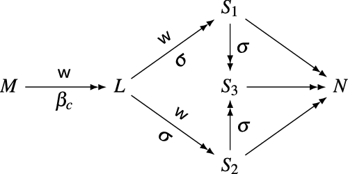
Figure 4: Surface reduction.
To prove (#), we show that the sequences
![]() and
and
![]() have the same number of βc steps.
have the same number of βc steps.
By confluence of
![]() (Proposition 5.5.1),
(Proposition 5.5.1),
![]() , for some
, for some
![]() , and (by confluence of
, and (by confluence of
![]() , Proposition 5.5.2) there is a sequence
, Proposition 5.5.2) there is a sequence
![]() . By Lemma 8.2, since
. By Lemma 8.2, since
![]() are
are
![]() -normal, terms in these sequences are
-normal, terms in these sequences are
![]() -normal, and so all steps are not only surface, but also
-normal, and so all steps are not only surface, but also
![]() steps. That is,
steps. That is,
![]() ,
,
![]() and
and
![]() . Hence,
. Hence,
![]() have the same shape by Fact 6.2.
have the same shape by Fact 6.2.
We examine the shape of N, and prove claim (#) by showing that
![]() and
and
![]() have the same number of βc steps as
have the same number of βc steps as
![]() (note that the sequences
(note that the sequences
![]() and
and
![]() have no βc steps).
have no βc steps).
•
![]() . In this case,
. In this case,
![]() , and the claim (#) is immediate.
, and the claim (#) is immediate.
•
![]() , and
, and
![]() . We have
. We have
![]() and
and
![]() . Since P and Q are
. Since P and Q are
![]() -normal, by i.h. we have:
-normal, by i.h. we have:
- the two sequences
![]() and
and
![]() have the same number of βc steps, and similarly
have the same number of βc steps, and similarly
![]() and
and
![]() . Hence,
. Hence,
![]() and
and
![]() have the same number of βc steps.
have the same number of βc steps.
- Similarly,
![]() and
and
![]() have the same number of βc steps.
have the same number of βc steps.
This completes the proof of (#). We now can conclude that
![]() is uniformly normalizing. If the term M has a sequence
is uniformly normalizing. If the term M has a sequence
![]() where N is
where N is
![]() -normal, then no
-normal, then no
![]() -sequence can have more βc steps than
-sequence can have more βc steps than
![]() , because given any sequence
, because given any sequence
![]() then (by confluence of
then (by confluence of
![]() )
)
![]() , and (by #)
, and (by #)
![]() has the same number of βc steps as
has the same number of βc steps as
![]() . Hence, all
. Hence, all
![]() -sequences from M are finite.
-sequences from M are finite.![]()
Normalizing strategies
We are ready to define and deal with normalizing strategies for λ©. Our definition is inspired, and generalizes, the stratified strategy proposed in Guerrieri (Reference Guerrieri2015), Guerrieri et al. (Reference Guerrieri, Paolini and Ronchi Della Rocca2017), which iterates weak reduction (there called head reduction) according to a more strict discipline.
Iterated
![]() -Reduction. We define a family of normalizing strategies, parametrically on the reduction to iterate, which can be surface or weak. Let
-Reduction. We define a family of normalizing strategies, parametrically on the reduction to iterate, which can be surface or weak. Let
![]() . Reduction
. Reduction
![]() is defined as follows, by iterating
is defined as follows, by iterating
![]() in the left-to-right order (Theorem 8.14 then shows that
in the left-to-right order (Theorem 8.14 then shows that
![]() is a normalizing strategy).
is a normalizing strategy).
(1) If M is not
![]() -normal:
-normal:

(2) If M is
![]() -normal (below, “
-normal (below, “
![]() -normal” means
-normal” means
![]() or
or
![]() with L βcσ-normal):
with L βcσ-normal):

Theorem 8.14 (Normalization for βcσ). Assume
![]() where N is
where N is
![]() -normal. Let
-normal. Let
![]() . Then, every maximal
. Then, every maximal
![]() -sequence from M ends in N.
-sequence from M ends in N.
Proof. By induction on the term N. Let
![]() be a maximal
be a maximal
![]() -sequence from M.
-sequence from M.
We write
,
,
and
for
, respectively. We observe that
Indeed, from
![]() , by
, by
![]() -factorization, we have that
-factorization, we have that
![]() . Since N is
. Since N is
![]() -normal, so is L (by Lemma 8.3) and (**) follows by uniform normalization of
-normal, so is L (by Lemma 8.3) and (**) follows by uniform normalization of
![]() (Theorem 8.13).
(Theorem 8.13).
Let
![]() be the maximal prefix of
be the maximal prefix of
![]() such that
such that
![]() . Since it is finite,
. Since it is finite,
![]() is
is
![]() , where
, where
![]() is
is
![]() -normal. Let
-normal. Let
![]() be the sequence such that
be the sequence such that
![]() .
.
Note that all terms in
![]() are
are
![]() -normal (by repeatedly using Lemma 8.3 from
-normal (by repeatedly using Lemma 8.3 from
![]() ), hence
), hence
![]() , and (by shape preservation, Fact 6.2) all terms in
, and (by shape preservation, Fact 6.2) all terms in
![]() have the same shape as
have the same shape as
![]() .
.
By confluence of
![]() (Proposition 5.9.2),
(Proposition 5.9.2),
![]() . Again, all terms in this sequence are
. Again, all terms in this sequence are
![]() -normal, by repeatedly using Lemma 8.3 from
-normal, by repeatedly using Lemma 8.3 from
![]() . So,
. So,
![]() , and (by shape preservation, Fact 6.2)
, and (by shape preservation, Fact 6.2)
![]() and N have the same shape.
and N have the same shape.
We have established that
![]() and all terms in
and all terms in
![]() have the same shape as N. Now we examine the possible cases for N.
have the same shape as N. Now we examine the possible cases for N.
•
![]() , and
, and
![]() . Trivially
. Trivially
![]() .
.
•
![]() and
and
![]() with
with
![]() . Since
. Since
![]() is βcσ-normal, by i.h. every maximal
is βcσ-normal, by i.h. every maximal
![]() -sequence from P terminates in
-sequence from P terminates in
![]() , and so every maximal
, and so every maximal
![]() -sequence from
-sequence from
![]() terminates in
terminates in
![]() . Since the sequence
. Since the sequence
![]() is a maximal
is a maximal
![]() -sequence, we have that
-sequence, we have that
![]() is as follows
is as follows
•
![]() and
and
![]() , with
, with
![]() and
and
![]() . Since
. Since
![]() and
and
![]() are both βcσ-normal, by i.h. :
are both βcσ-normal, by i.h. :
- every maximal
![]() -sequence from P ends in
-sequence from P ends in
![]() . So every
. So every
![]() -sequence from
-sequence from
![]() eventually reaches
eventually reaches
![]() ;
;
- every maximal
![]() -sequence from Q ends in
-sequence from Q ends in
![]() . So every
. So every
![]() -sequence from
-sequence from
![]() eventually reaches
eventually reaches
![]() .
.
Therefore
![]() is as follows
is as follows
•
![]() and
and
![]() . Similar to the previous one.
. Similar to the previous one.![]()
From a normalizing strategy for
![]() (Theorem 8.14), we derive a normalizing strategy in λ©.
(Theorem 8.14), we derive a normalizing strategy in λ©.
Corollary 8.15 (Normalization for λ©) Let
![]() . If M is ©-normalizing, then any maximal
. If M is ©-normalizing, then any maximal
![]() -sequence from M followed by any maximal
-sequence from M followed by any maximal
![]() -sequence ends in the ©-normal form of M.
-sequence ends in the ©-normal form of M.
Proof. By Theorem 8.14, every maximal
![]() -sequence from M ends in a
-sequence from M ends in a
![]() -normal form L. Since
-normal form L. Since
![]() is strongly normalizing (Proposition 8.6), every maximal
is strongly normalizing (Proposition 8.6), every maximal
![]() -sequence from L ends in a
-sequence from L ends in a
![]() -normal form N, which is also
-normal form N, which is also
![]() -normal by Lemma 8.1. Therefore, N is ©-normal and this is the unique ©-normal form of M since
-normal by Lemma 8.1. Therefore, N is ©-normal and this is the unique ©-normal form of M since
![]() is confluent (Proposition 5.9.3).
is confluent (Proposition 5.9.3).![]()
9. Conclusions and Related Work
9.1 Discussion: reduction and evaluation
In computational calculi, it is standard practice to define evaluation as weak reduction, aka sequencing (Dal Lago et al. Reference Dal Lago, Gavazzo and Levy2017; Filinski Reference Filinski1996; Jones et al. Reference Jones, Shields, Launchbury, Tolmach, MacQueen and Cardelli1998; Levy et al. Reference Levy, Power and Thielecke2003). Despite the prominent role that weak reduction has in the literature, in particular for calculi with effects, what one discovers when analyzing the rewriting properties is somehow unexpected. As we observe in Section 5, where we consider both the computational core λ© (de' Liguoro and Treglia 2020), and a widely recognized reference such as the calculus
![]() by Sabry and Wadler (Reference Sabry and Wadler1997) (in turn inspired by Moggi Reference Moggi1988, Reference Moggi1989, Reference Moggi1991), while full reduction is confluent, the closure of the rules under evaluation contexts turns out to be non-deterministic, non-confluent, and its normal forms are not unique. The issues come from the monadic rules of identity and associativity, hence they are common to all computational calculi.
by Sabry and Wadler (Reference Sabry and Wadler1997) (in turn inspired by Moggi Reference Moggi1988, Reference Moggi1989, Reference Moggi1991), while full reduction is confluent, the closure of the rules under evaluation contexts turns out to be non-deterministic, non-confluent, and its normal forms are not unique. The issues come from the monadic rules of identity and associativity, hence they are common to all computational calculi.
A Bridge between Evaluation and Reduction. On the one hand, computational λ-calculi have an unrestricted non-deterministic reduction that generates the equational theory of the calculus, studied for foundational and semantic purposes. On the other hand, weak reduction models evaluation in an ideal programming language. It is then natural to wonder what is the relation between reduction and evaluation. This is the first contribution of this paper. We establish a bridge between evaluation and reduction via a factorization theorem stating that every reduction can be rearranged so as to bring forward weak reduction steps.
We focused on the rewriting theory of a specific computational calculus, namely the computational core λ© (de' Liguoro and Treglia 2020). We expect that our results and approach can be adapted also to other computational calculi such as
![]() . This demands further investigations. Transferring the results is not immediate because the correspondence between the two calculi is not direct with respect to the rewriting (see Remark 3.10).
. This demands further investigations. Transferring the results is not immediate because the correspondence between the two calculi is not direct with respect to the rewriting (see Remark 3.10).
9.2 Technical contributions
We studied the rewriting theory of the computational core λ© introduced in de' Liguoro and Treglia (2020), a variant of Moggi’s λc-calculus Moggi (Reference Moggi1988), focusing on two questions:
• how to reach values?
• how to reach normal forms?
For the first point, we show that weak βc-reduction is enough (Section 7). For the second question, we define a family of normalizing strategies (Section 8).
We have faced the issues caused by identity and associativity rules (which internalize the monadic rules in the syntax) and dealt with them by means of factorization techniques.
We have investigated in depth the structure of normalizing reductions, and we assessed the role of the σ-rule (aka associativity) as computational and not merely structural. We found out that it plays at least three distinct, independent roles in λ©:
• σ unblocks “premature” βc-normal forms so as to guarantee that there are not ©-normalizing terms whose semantics is the same as diverging terms, as we have seen in Section 8.2;
• it internalizes the associativity of Kleisli composition into the calculus, as a syntactic reduction rule, as explained in Section 1 after Equation (3);
• it “simulates” the contextual closure of the βc-rule for terms that reduce to a value, as we have seen in Theorem 7.4.
9.3 Related work
Relation with Moggi’s Calculus. Since our focus is on operational properties and reduction theory, we chose the computational core λ© (de' Liguoro and Treglia 2020) among the different variants of computational calculi in the literature inspired by Moggi’s seminal work (Moggi 1988 Reference Moggi1989, Reference Moggi1991). Indeed, the computational core λ© has a “minimal” syntax that internalizes Moggi’s original idea of deriving a calculus from the categorical model consisting of the Kleisli category of a (strong) monad. For instance, λ© does not have to consider both a pure and a (potentially) effectful functional application. So, λ© has less syntactic constructors and less reductions rules with respect to other computational calculi, and this simplifies our operational study.
Let us discuss the difference between λ© and Moggi’s λc. As observed in Sections 1 and 3, the first formulation of λc and of its reduction relation was introduced in Moggi (Reference Moggi1988), where it is formalized by using let-constructor. Indeed, this operator is not just a syntactical sugar for the application of λ-abstraction. In fact, it represents the extension to computations of functions from values to computations, therefore interpreting Kleisli composition. Combining let with ordinary abstraction and application is at the origin of the complexity of the reduction rules in Moggi (Reference Moggi1988). On the other hand, this allows extensionality to be internalized. Adding the η-rule to λ© breaks confluence, as shown in de' Liguoro and Treglia (2020).
Besides using let or not, a major difference of λ© with respect to λc is the neat distinction among the two syntactical sorts of terms, restricting the combination of values and non-values since the very definition of the grammar of the language. In spite of these differences, in de' Liguoro and Treglia (2019, Section 9) it has been proved that there exists an interpretation of λc into λ© that preserves the reduction, while there is a reverse translation that preserves convertibility, only.
Other Related Work. Sabry and Wadler (Reference Sabry and Wadler1997) is the first work on the computational calculus to put on center stage the reduction. Still the focus of the paper are the properties of the translation between that and the monadic metalanguage – the reduction theory itself is not investigated.
In Herbelin and Zimmermann (Reference Herbelin, Zimmermann and Curien2009) a different refinement of λc has been proposed. Its reduction rules are divided into a purely operational, a structural and an observational system. It is proved that the purely operational system suffices to reduce any closed term to a value. This result is similar to our Theorem 7.6, with weak βc steps corresponding to head reduction in Herbelin and Zimmermann (Reference Herbelin, Zimmermann and Curien2009). Interestingly, the analogous of our rule σ is part of the structural system, while the rule corresponding to our
![]() is generalized and considered as an observational rule. Unlike our work, normalization is not studied in Herbelin and Zimmermann (Reference Herbelin, Zimmermann and Curien2009).
is generalized and considered as an observational rule. Unlike our work, normalization is not studied in Herbelin and Zimmermann (Reference Herbelin, Zimmermann and Curien2009).
Surface reduction is a generalization of weak reduction that comes from linear logic. We inherit surface factorization from the linear λ-calculus in Simpson (Reference Simpson and Giesl2005). Such a reduction has been recently studied in several variants of the λ-calculus, especially for semantic purposes (Accattoli and Guerrieri Reference Accattoli and Guerrieri2016; Accattoli and Paolini Reference Accattoli and Paolini2012; Bucciarelli et al. Reference Bucciarelli, Kesner, Ros, Viso, Nakano and Sagonas2020; Carraro and Guerrieri Reference Carraro and Guerrieri2014; Ehrhard and Guerrieri Reference Ehrhard and Guerrieri2016; Guerrieri and Manzonetto Reference Guerrieri and Manzonetto2019; Guerrieri and Olimpieri Reference Guerrieri and Olimpieri2021; Guerrieri Reference Guerrieri2019).
Regarding the σ-rule, in Carraro and Guerrieri (Reference Carraro and Guerrieri2014) two commutation rules are added to Plotkin’s CbV λ-calculus in order to remove meaningless normal forms – the resulting calculus is called shuffling. The commutative rule there called
![]() is literally the same as σ here. In the setting of the shuffling calculus, properties such as the fact that all maximal surface
is literally the same as σ here. In the setting of the shuffling calculus, properties such as the fact that all maximal surface
![]() -reduction sequences from the same term M have the same number of
-reduction sequences from the same term M have the same number of
![]() steps, and so such a reduction is uniformly normalizing, were known via semantic tools (Carraro and Guerrieri Reference Carraro and Guerrieri2014; Guerrieri Reference Guerrieri2019), namely non-idempotent intersection types. In this paper, we give the first syntactic proof of such a result.
steps, and so such a reduction is uniformly normalizing, were known via semantic tools (Carraro and Guerrieri Reference Carraro and Guerrieri2014; Guerrieri Reference Guerrieri2019), namely non-idempotent intersection types. In this paper, we give the first syntactic proof of such a result.
A relation between the computational calculus, Simpson (Reference Simpson and Giesl2005) and other linear calculi are well known in the literature, see for example Egger et al. (Reference Egger, Møgelberg, Simpson, Grädel and Kahle2009), Sabry and Wadler (Reference Sabry and Wadler1997), Maraist et al. (Reference Maraist, Odersky, Turner and Wadler1999).
In de' Liguoro and Treglia (2020), Theorem 8.4 states that any closed term returns a value if and only if it is convergent according to a big-step operational semantics. That proof is incomplete and needs a more complex argument via factorization, as we do here to prove Theorem 7.6 (from which that statement in de’ Liguoro and Treglia Reference de’ Liguoro and Treglia2020 easily follows).
Acknowledgements. We are in debt with Vincent van Oostrom, for the technical issues he pinpointed, and for his many insightful technical suggestions. We also thank the referees for their valuable comments. This work was partially supported by the ANR project PPS: ANR-19-CE48-0014.
Note
Precisely, Accattoli studies the relation between the kernel calculus
![]() and the value substitution calculus
and the value substitution calculus
![]() , i.e. CbV and the kernel extended with explicit substitutions. The syntax is slightly different, but not in an essential way.
, i.e. CbV and the kernel extended with explicit substitutions. The syntax is slightly different, but not in an essential way.
APPENDIX
APPENDIX A. General properties of the contextual closure
Shape Preservation. We start by recalling a basic but key property of contextual closure. If a step
![]() is obtained by closure under non-empty context of a rule
is obtained by closure under non-empty context of a rule
![]() , then it preserves the shape of the term. We say that T and T’ have the same shape if both terms are an application (resp. an abstraction, an variable, a term of shape
, then it preserves the shape of the term. We say that T and T’ have the same shape if both terms are an application (resp. an abstraction, an variable, a term of shape
![]() ).
).
Fact 6.2. (Shape preservation). Let
![]() be a rule and
be a rule and
![]() be its contextual closure. Assume
be its contextual closure. Assume
![]() where
where
![]() and
and
![]() Then T and
Then T and
![]() have the same shape.
have the same shape.
Note that a root step
![]() is both a weak and a surface step.
is both a weak and a surface step.
The implication in the previous lemma cannot be reversed as the following example shows:
M is a σ-redex, but N is not.
Substitutivity. A relation
![]() on terms is substitutive if
on terms is substitutive if
An obvious induction on the shape of terms shows the following Barendregt (Reference Barendregt1984, p. 54).
Fact A.1 (Substitutive) Let
![]() be the contextual closure of
be the contextual closure of
![]() .
.
(1) If
![]() is substitutive then
is substitutive then
![]() is substitutive:
is substitutive:
![]() implies
implies
![]() .
.
(2) If
![]() then
then
![]() .
.
APPENDIX B. Properties of the syntax
In this section, we consider the set of terms
![]() (the same syntax as the full bang calculus, as defined in Section 4), endowed with a generic reduction
(the same syntax as the full bang calculus, as defined in Section 4), endowed with a generic reduction
![]() (from a generic rule
(from a generic rule
![]() ). We study some properties that hold in general in
). We study some properties that hold in general in
![]() .
.
Terms are generated by the grammar:
Contexts (
![]() ), surface contexts (
), surface contexts (
![]() ) and weak contexts (
) and weak contexts (
![]() ) are generated by the grammars:
) are generated by the grammars:
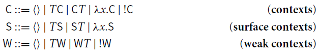
If
![]() is a rule, the reduction
is a rule, the reduction
![]() its the closure under context
its the closure under context
![]() . Surface reduction
. Surface reduction
![]() (resp. weak reduction
(resp. weak reduction
![]() ) is the closure of
) is the closure of
![]() under surface contexts
under surface contexts
![]() (resp. weak contexts
(resp. weak contexts
![]() ). Non-surface reduction
). Non-surface reduction
![]() (resp. non-weak reduction
(resp. non-weak reduction
![]() ) is the closure of
) is the closure of
![]() under contexts
under contexts
![]() that are not surface (resp. not weak).
that are not surface (resp. not weak).
B.1 Shape preservation for internal steps in .
Fact 6.2 (p. 19) implies that
![]() and
and
![]() steps always preserve the shape of terms. We recall that we write
steps always preserve the shape of terms. We recall that we write
![]() to indicate the step
to indicate the step
![]() obtained by empty contextual closure. The following property immediately follows from Fact 6.2.
obtained by empty contextual closure. The following property immediately follows from Fact 6.2.
Fact B.1 (Internal Steps) Let
![]() be a rule and
be a rule and
![]() be its contextual closure. The following hold for
be its contextual closure. The following hold for
![]() .
.
(1) Reduction
![]() preserves the shapes of terms.
preserves the shapes of terms.
(2) There is no T such that
![]() , for any variable x.
, for any variable x.
(3)
![]() implies
implies
![]() and
and
![]() .
.
(4)
![]() implies
implies
![]() and
and
![]() .
.
(5)
![]() implies
implies
![]() , with either (i)
, with either (i)
![]() (and
(and
![]() ) or (ii)
) or (ii)
![]() (and
(and
![]() ). Moreover,
). Moreover,
![]() and
and
![]() have the same shape, and so
have the same shape, and so
![]() and
and
![]() .
.
Corollary B.2. Let
![]() be a rule and
be a rule and
![]() be its contextual closure. Assume
be its contextual closure. Assume
![]() or
or
![]() .
.
• T is a
![]() -redex if and only if S is.
-redex if and only if S is.
• T is a σ-redex if and only if S is.
Proof. The left-to-right direction follows from Fact B.1.1. The right-to-left direction is obtained by repetitively applying Fact B.1.3-5.![]()
B.2 Surface Factorization, Modularly
In an abstract setting, let us consider a rewrite system
![]() where
where
![]() . Under which condition
. Under which condition
![]() admits factorization, assuming that both
admits factorization, assuming that both
![]() and
and
![]() do? That is, if
do? That is, if
![]() and
and
![]()
![]() -factorize ( i.e.
-factorize ( i.e.
![]() and
and
![]() ), is it the case that
), is it the case that
![]() (where
(where
![]() and
and
![]() )? To deal with this question, a technique for proving factorization for compound systems in a modular way has been introduced in Accattoli et al. (Reference Accattoli, Faggian and Guerrieri2021). The approach can be seen as an analog – for factorization – of the classical technique for confluence based on Hindley–Rosen lemma: if
)? To deal with this question, a technique for proving factorization for compound systems in a modular way has been introduced in Accattoli et al. (Reference Accattoli, Faggian and Guerrieri2021). The approach can be seen as an analog – for factorization – of the classical technique for confluence based on Hindley–Rosen lemma: if
![]() are
are
![]() -factorizing reductions, their union
-factorizing reductions, their union
![]() also is, provided that two local conditions of commutation hold.
also is, provided that two local conditions of commutation hold.
Theorem B.3 (Modular factorization, abstractly Accattoli et al. Reference Accattoli, Faggian and Guerrieri2021). Let
![]() and
and
![]() be
be
![]() -factorizing reductions. Let
-factorizing reductions. Let
![]() , and
, and
![]() . The union
. The union
![]() satisfies factorization
satisfies factorization
![]() if the following swaps hold
if the following swaps hold
Extensions of the bang calculus. Following Faggian and Guerrieri (Reference Faggian and Guerrieri2021), we now consider a calculus
![]() , where
, where
![]() and
and
![]() is the contextual closure of a new rule
is the contextual closure of a new rule
![]() . Theorem B.3 states that the compound system
. Theorem B.3 states that the compound system
![]() satisfies surface factorization if
satisfies surface factorization if
![]() ,
,
![]() , and the two linear swaps hold. We know that
, and the two linear swaps hold. We know that
![]() always hold. We now show that verifying the linear swaps reduces to a single simple test, leading to Proposition 6.5.
always hold. We now show that verifying the linear swaps reduces to a single simple test, leading to Proposition 6.5.
First, we observe that each linear swap condition can be tested by considering for the surface step only
![]() , that is, only the closure of
, that is, only the closure of
![]() under empty context. This is expressed in the following lemma, where we include also a useful variant.
under empty context. This is expressed in the following lemma, where we include also a useful variant.
Lemma B.4 (Root linear swaps). In
![]() , let
, let
![]() be the contextual closure of rules
be the contextual closure of rules
![]() .
.
(1)
![]() implies
implies
![]() .
.
(2) Similarly,
![]() implies
implies
![]() .
.
Proof. Assume
![]() . If U is the redex, the claim holds by assumption. Otherwise, we prove
. If U is the redex, the claim holds by assumption. Otherwise, we prove
![]() , by induction on the structure of U . Observe that both M and N have the same shape as U (by Property 6.2).
, by induction on the structure of U . Observe that both M and N have the same shape as U (by Property 6.2).
•
![]() (hence
(hence
![]() and
and
![]() ). We have two cases.
). We have two cases.
(1) Case
![]() . By Fact B.1, either
. By Fact B.1, either
![]() or
or
![]() .
.
a. Assume
![]() .
.
We have
![]() , and we conclude by i.h. .
, and we conclude by i.h. .
b. Assume
![]() .
.
Then
![]() .
.
(2) Case
![]() . Similar to the above.
. Similar to the above.
•
![]() (hence
(hence
![]() and
and
![]() ). We conclude by i.h. .
). We conclude by i.h. .
Cases
![]() or
or
![]() do not apply.
do not apply.![]()
As we study
![]() , one of the linear swap is
, one of the linear swap is
![]() . We show that any
. We show that any
![]() linearly swaps after
linearly swaps after
![]() as soon as
as soon as
![]() is substitutive.
is substitutive.
Lemma B.5 (Swap with
![]() ). If
). If
![]() is substitutive, then
is substitutive, then
![]() always holds.
always holds.
Proof. We prove
![]() , and conclude by Lemma B.4.
, and conclude by Lemma B.4.
Assume
![]() . We want to prove
. We want to prove
![]() . By Fact B.1,
. By Fact B.1,
![]() and either
and either
![]() or
or
![]() .
.
• In the first case,
![]() , with
, with
![]() . So,
. So,
![]() and we conclude by substitutivity of
and we conclude by substitutivity of
![]() (Fact A.1.1).
(Fact A.1.1).
• In the second case,
![]() with
with
![]() . Therefore,
. Therefore,
![]() , and we conclude by Fact A.1.2.
, and we conclude by Fact A.1.2.![]()
Summing up, since surface factorization for
![]() is known, we obtain the following compact test for surface factorization in extensions of
is known, we obtain the following compact test for surface factorization in extensions of
![]() .
.
Proposition B.6 (A modular test for surface factorization). Let
![]() be
be
![]() -reduction and
-reduction and
![]() be the contextual closure of a rule
be the contextual closure of a rule
![]() . The reduction
. The reduction
![]() satisfies surface factorization if:
satisfies surface factorization if:
(1) Surface factorization of
![]() :
:
![]()
(2)
![]() is substitutive:
is substitutive:
![]()
(3) Root linear swap:
![]() .
.
B.3 Restriction to computations
In
![]() , let
, let
![]() be a rule and
be a rule and
![]() be its contextual closure. The restriction of reduction to computations preserves
be its contextual closure. The restriction of reduction to computations preserves
![]() steps. Thus, all properties that hold for
steps. Thus, all properties that hold for
![]() (e.g. Fact B.1 and Corollary B.2) also hold for
(e.g. Fact B.1 and Corollary B.2) also hold for
![]() .
.
In particular, Proposition 6.5 is immediate consequence of Proposition B.6.
APPENDIX C. Properties of reduction in λ©
We now consider λ©, that is
![]() . As we have just seen above, the properties we have studied in Appendix B also hold when restricting reduction to computations. Moreover, λ© satisfies also specific properties that do not hold in general, as the following.
. As we have just seen above, the properties we have studied in Appendix B also hold when restricting reduction to computations. Moreover, λ© satisfies also specific properties that do not hold in general, as the following.
Lemma C.1. Let
![]() and
and
![]() : M is a
: M is a
![]() -redex (resp. a ι-redex) if and only if L is.
-redex (resp. a ι-redex) if and only if L is.
Proof. If M is a
![]() -redex, this means that
-redex, this means that
![]() where
where
![]() , hence L is a
, hence L is a
![]() -redex. Moreover, if M is a ι-redex, then
-redex. Moreover, if M is a ι-redex, then
![]() , hence by Fact B.1
, hence by Fact B.1
![]() for any V’. Thus L is a ι-redex.
for any V’. Thus L is a ι-redex.
Let us prove that if L is a
![]() -redex, so is M. Since
-redex, so is M. Since
![]() , by Fact B.1, M is an application; we have the following cases:
, by Fact B.1, M is an application; we have the following cases:
(i) either
![]() where
where
![]() ;
;
(ii) or
![]() where
where
![]() .
.
Case (i.) is impossible because otherwise
![]() for some value V, by Fact B.1, such that
for some value V, by Fact B.1, such that
![]() , but such a V does not exist. Therefore, we are necessarily in case (ii.), i.e., M is a
, but such a V does not exist. Therefore, we are necessarily in case (ii.), i.e., M is a
![]() -redex. Moreover, if L is a ι-redex, then
-redex. Moreover, if L is a ι-redex, then
![]() , hence N is an application, and so is P by Fact B.1.
, hence N is an application, and so is P by Fact B.1.![]()
Note that Lemma C.1 is false if we replace the hypothesis
![]() with
with
![]() . Indeed, consider
. Indeed, consider
![]() : L is a
: L is a
![]() -redex but M is not.
-redex but M is not.
Lemma C.2. There is no
![]() such that
such that
![]() .
.
Proof. By induction on
![]() , proving that for every M such that
, proving that for every M such that
![]() ,
,
![]() .
.![]()
C.1 Postponement of ι, Technical Lemmas
Lemma C.3 (ι vs. β 1).
![]()
Proof. We set the notation
![]() .
.
The proof is by induction on L. Cases:
•
![]() . Then, there are two possibilities.
. Then, there are two possibilities.
Either
![]() then
then
Or
![]() with
with
![]() , and then
, and then
The case
![]() with
with
![]() is impossible by Lemma C.2.
is impossible by Lemma C.2.
•
![]() where
where
![]() . In this case note that necessarily
. In this case note that necessarily
![]() where
where
![]() . Otherwise, it should have been
. Otherwise, it should have been
![]() , but the ι step is impossible because
, but the ι step is impossible because
![]() . By i.h. , since
. By i.h. , since
![]() , we have
, we have
![]() ; hence
; hence
![]() .
.
•
![]() where
where
![]() is not root steps, that is:
is not root steps, that is:
(a) either
![]() and
and
![]() ;
;
(b) or
![]() and
and
![]() .
.
By Fact 6.2, M, L, N are applications. So, M has the following shape:
(1)
![]() with
with
![]()
(2)
![]() with
with
![]()
(3)
![]()
We distinguish six sub-cases:
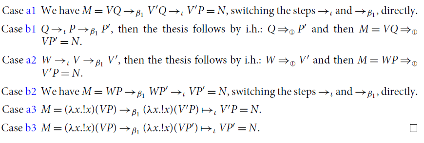
Lemma C.4 (ι vs.
![]() ).
).
![]()
Proof. We set the notation
![]() . The proof is by induction on L. Note that if
. The proof is by induction on L. Note that if
![]() there is no
there is no
![]() reduction from it, so this case is not in the scope of the induction. Cases:
reduction from it, so this case is not in the scope of the induction. Cases:
•
![]() . Then, there are three possibilities.
. Then, there are three possibilities.
(i)
![]() with
with
![]()
(ii)
![]() with
with
![]()
(iii)
![]()
So by analyzing each of the three cases above, we can postpone the
![]() step as follows:
step as follows:
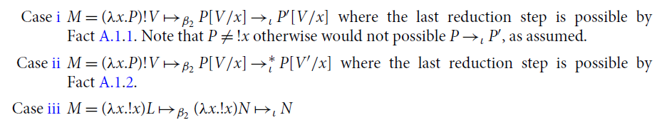
•
![]() where
where
![]() . In this case, note that M has necessary the shape
. In this case, note that M has necessary the shape
![]() where
where
![]() . Otherwise, M should have been
. Otherwise, M should have been
![]() , but it is impossible by definition of
, but it is impossible by definition of
![]() since
since
![]() . The thesis follows by induction, since we have
. The thesis follows by induction, since we have
![]()
![]() .
.
•
![]() where
where
![]() is not root steps, that is:
is not root steps, that is:
(a) either
![]() and
and
![]() ;
;
(b) or
![]() and
and
![]() .
.
By Fact 6.2, M, L, N are applications. So, M has the following shape:
(1)
![]() with
with
![]()
(2)
![]() with
with
![]()
(3)
![]()
We distinguish six subcases:
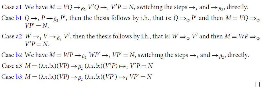
Lemma C.5 (ι vs. σ).
![]()
Proof. We set the notation
![]() .
.
The proof is by induction on L. We distinguishing if the last
![]() is a root step or not.
is a root step or not.
If
![]() , then
, then
![]() and
and
![]() . Thus, there are seven cases for M:
. Thus, there are seven cases for M:
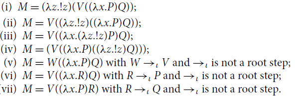
So by analyzing each of the seven cases above, we can postpone the
![]() step as follows:
step as follows:
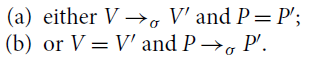
Consider the case
![]() with
with
![]() . So, note that M has necessary the shape
. So, note that M has necessary the shape
![]() where
where
![]() . Otherwise, M should have been
. Otherwise, M should have been
![]() , but it is impossible by definition of
, but it is impossible by definition of
![]() since
since
![]() . The thesis follows by i.h. , since
. The thesis follows by i.h. , since
![]() .
.
The last case to consider is
![]() where
where
![]() is not root steps, that is:
is not root steps, that is:
By Fact 6.2, M, L, N are applications. So, M has one of the following shapes:
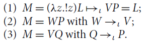
Hence, combining Points a and b with Points 1 to 3, we distinguish six subcases:
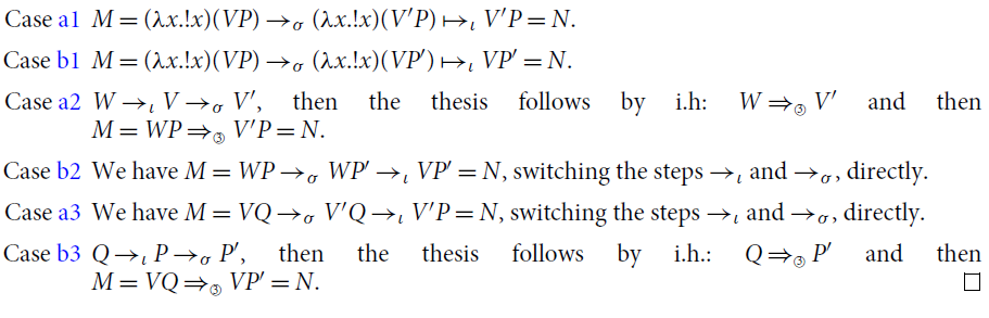
APPENDIX D. Normalization of λ©
Lemma 8.3. Let
![]() . If
. If
![]() N then:
N then:
![]() - normal if and only if N is
- normal if and only if N is
![]() - normal.
- normal.
Proof. By easy induction on the shape of M. Observe that M and N have the same shape because the step
![]() is not a root step.
is not a root step.
•
![]() and
and
![]() : the claim is trivial.
: the claim is trivial.
•
![]() and
and
![]() . Either
. Either
![]() (and
(and
![]() ) or
) or
![]() (and
(and
![]() ). Assume M = VP is
). Assume M = VP is
![]() -normal. Since V and P are
-normal. Since V and P are
![]() -normal, by i.h. so are V’ and P’. Moreover, N is not a redex, by Corollary B.2, so N is normal. Assuming
-normal, by i.h. so are V’ and P’. Moreover, N is not a redex, by Corollary B.2, so N is normal. Assuming
![]() normal is similar.
normal is similar.![]()
Fact D.1. The reduction ι is quasi-diamond. Therefore, if ![]() where N is ι-normal, then any maximal ι-sequence from S ends in N, in k steps.
where N is ι-normal, then any maximal ι-sequence from S ends in N, in k steps.
Lemma 8.1. Assume
![]() .
.
(1) M is β c -normal if and only if N is β c -normal.
(2) If M is σ-normal, so is N.
Proof. Easy to prove by induction on the structure of terms.![]()
Fact D.2 (Shape preservation of ι-sequences). If S is not an ι-redex, and
![]() then no term in the sequence is an ι-redex, and so N has the same shape as S:
then no term in the sequence is an ι-redex, and so N has the same shape as S:
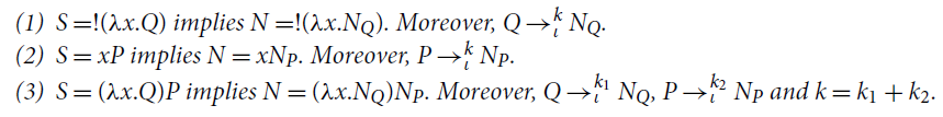
Lemma 8.5. Assume
![]() , where
, where
![]() , and N is
, and N is
![]() -normal. If M is not
-normal. If M is not
![]() -normal, then there exist
-normal, then there exist
![]() and
and
![]() such that either
such that either
![]() or
or
![]() .
.
Proof. The proof is by induction on M.
Assume M is a is a σ-redex, i.e.
![]() where V is an abstraction.
where V is an abstraction.
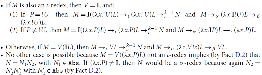
Assume M is not a σ-redex. We examine the shape of S and use Fact D.2.
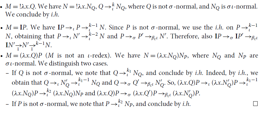
Proposition 8.6. (Termination of
![]() ). Reduction
). Reduction
![]() is strongly normalizing.
is strongly normalizing.
Proof. We define two sizes
![]() and
and
![]() for any term M.
for any term M.
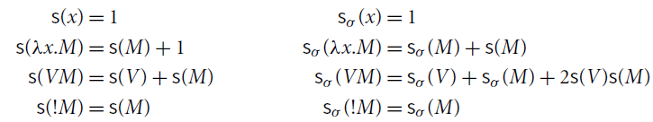
Note that
![]() and
and
![]() for any term M. It easy to check that if
for any term M. It easy to check that if
![]() , then
, then
![]() , where
, where
![]() is the strict lexicographical order on
is the strict lexicographical order on
![]() . Indeed, if
. Indeed, if
![]() , then
, then
![]() ; and if
; and if
![]() then
then
![]() and
and
![]() . The proof is by straightforward induction on M. We show only the root cases, the other cases follow from the i.h. immediately.
. The proof is by straightforward induction on M. We show only the root cases, the other cases follow from the i.h. immediately.
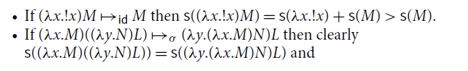
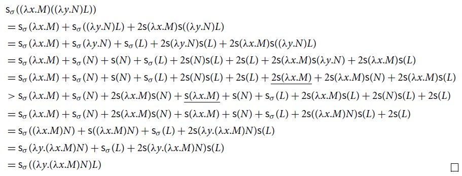
APPENDIX E. Notational Equivalence between λ© and de' Liguoro and Treglia (2020)
Here we recall the calculus introduced in de' Liguoro and Treglia (2020) (see also our Section 1), henceforth denoted by
![]() , and formalize that
, and formalize that
![]() is isomorphic to the computational core λ©. In other words, λ© (as defined in Section 3) is nothing but another presentation of
is isomorphic to the computational core λ©. In other words, λ© (as defined in Section 3) is nothing but another presentation of
![]() , with just a different notation.
, with just a different notation.
First, we recall the syntax of
![]() , with
, with
![]() and
and
![]() operators:
operators:
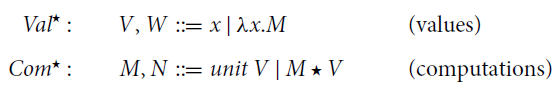
We set
![]() . Contexts are defined in Section 1. Reductions in
. Contexts are defined in Section 1. Reductions in
![]() are the contextual closures of the rules (1), (2), and (3) on p. 2, oriented left-to-right, giving rise to reductions
are the contextual closures of the rules (1), (2), and (3) on p. 2, oriented left-to-right, giving rise to reductions
![]() ,
,
![]() , and
, and
![]() , respectively. We set
, respectively. We set
![]() .
.
Consider the translation
![]() from
from
![]() to
to
![]() , and conversely, the translation
, and conversely, the translation
![]() from
from
![]() to
to
![]() :
:
Table E1: Translations between λ© and
![]()
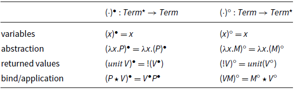
Essentially, translating terms of
![]() in terms of the computational core λ© rewrites
in terms of the computational core λ© rewrites
![]() as
as
![]() , and reverts the order in
, and reverts the order in
![]() .
.
Proposition E.1. The following holds:
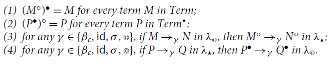
Table F1: Translations between the computational core λ© and the kernel of the Call-by-Value λ-calculus

Proof. Immediate by definition unfolding.
APPENDIX F. Computational versus Call-by-Value
Here we formalize the relation between a fragment of the computational core λ© and Plotkin’s call-by-value (CbV, for short) λ-calculus (Plotkin Reference Plotkin1975).
The fragment of λ© that includes just βc as only reduction rule, i.e.
![]() , is also isomorphic to the kernel of Plotkin’s CbV λ-calculus, which is the restriction of
, is also isomorphic to the kernel of Plotkin’s CbV λ-calculus, which is the restriction of
![]() (see Section 2.2) to the set of terms
(see Section 2.2) to the set of terms
![]() defined as follows (note that
defined as follows (note that
![]() ).
).
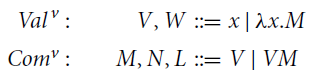
To establish such an isomorphism, consider the translation
![]() from
from
![]() to
to
![]() , and conversely, the translation
, and conversely, the translation
![]() from
from
![]() to
to
![]() .
.
Essentially, the translation
![]() simply forgets the operator
simply forgets the operator
![]() , and dually the translation
, and dually the translation
![]() adds a
adds a
![]() in front of each value that is not in the functional position of an application. These two translations form an isomorphism.
in front of each value that is not in the functional position of an application. These two translations form an isomorphism.
Proposition F.1.
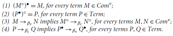
Proof. Immediate by definition unfolding.![]()
Observe also that the restriction of weak context to
![]() give exactly the grammar defined in Section 3, and this for all three weak contexts (
give exactly the grammar defined in Section 3, and this for all three weak contexts (
![]() ), which all collapse in the same shape. Thus, Proposition F.1 also holds when
), which all collapse in the same shape. Thus, Proposition F.1 also holds when
![]() and
and
![]() are replaced by
are replaced by
![]() and
and
![]() , respectively. As a consequence, since
, respectively. As a consequence, since
![]() is deterministic in
is deterministic in
![]() and
and
![]() weak factorizes (Theorem 2.11.1),
weak factorizes (Theorem 2.11.1),
Fact F.2 (Properties of βc and its restriction). In λ©:
• reduction
![]() is deterministic;
is deterministic;
• reduction
![]() satisfies weak factorization:
satisfies weak factorization:
![]() .
.
Call-by-Value versus its Kernel. The CbV kernel – and so
![]() – is as expressive as the CbV λ-calculus, as we discuss below. This result was already shown by Accattoli (Reference Accattoli2015).1
– is as expressive as the CbV λ-calculus, as we discuss below. This result was already shown by Accattoli (Reference Accattoli2015).1
With respect to its kernel, Plotkin’s CbV λ-calculus is more liberal in that application is unrestricted (left-hand side need not be a value). The kernel has the same expressive power as CbV calculus because the full syntax of Plotkin’s CbV can be encoded into the restricted one the CbV kernel and because the CbV kernel can simulate every reduction sequence of Plotkin’s full CbV.
Formally, consider the translation
![]() from Plotkin’s CbV λ-calculus to its kernel.
from Plotkin’s CbV λ-calculus to its kernel.
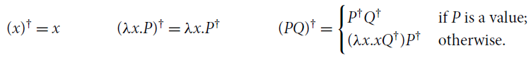
Proposition F.3 (Simulation of the CbV λ-calculus into its kernel). For every term P in Plotkin’s CbV λ-calculus, if
![]() then
then
![]() and
and
![]() .
.


 Open access