


1. Introduction
The two essential properties of a type theory, consistency and decidability of type checking, follow from three simpler ones: type preservation, strong normalization, and confluence. In dependent type theories, however, confluence is often needed to prove type preservation and strong normalization, making all three properties interdependent if termination is used in the confluence proof. This circularity can be broken in two ways: by proving all properties together within a single induction (Goguen Reference Goguen1994); or by proving confluence on untyped terms first, and then successively type preservation, confluence on typed terms, and strong normalization. We develop the latter way here, focusing on untyped confluence.
In a previous paper, we have investigated the case of a terminating set of left-linear rules for which critical pairs can be shown joinable by using rules from ${\mathcal{R}}$
. In the same paper, we explained that allowing us the use of arbitrary
${\mathcal{R}}$
. In the same paper, we explained that allowing us the use of arbitrary $\beta$
-steps for joining critical pairs would require a more complex notion of critical pair, and that parallel critical pairs cannot suffice in general. The goal of this paper is therefore to address the case of possibly non-terminating left-linear rules, or of terminating left-linear rules whose critical pairs cannot be joined without using
$\beta$
-steps for joining critical pairs would require a more complex notion of critical pair, and that parallel critical pairs cannot suffice in general. The goal of this paper is therefore to address the case of possibly non-terminating left-linear rules, or of terminating left-linear rules whose critical pairs cannot be joined without using $\beta$
-steps.
$\beta$
-steps.
Because beta reductions do not terminate for pure lambda terms, and rewrite rules may have critical pairs, the only available tool for proving confluence in this case is based on van Oostrom’s decreasing diagrams (van Oostrom Reference van Oostrom1994). Van Oostrom’s theorem is abstract: its application to non-terminating term rewriting relations conceals many difficulties, as is stressed in (Appel et al. Reference Appel, van Oostrom and Simonsen2010). An essential aspect of our methodology is to exhibit the rewrite relation for which confluence results from an analysis of its critical pairs. Here, this relation is orthogonal higher-order rewriting which pairs up nicely with beta reductions, whose confluence proof by Tait and Martin Löf was actually based on a dedicated notion of orthogonal reductions that they called parallel. A general notion of orthogonal rewriting was introduced in (Terese 2003), called multi-step rewriting. Multi-step rewriting aims at overcoming the limitations of left-linear, critical pair free rewriting systems introduced in (Huet and Lévy Reference Huet and Lévy1991), also called orthogonal systems. The main idea is to package several rewriting steps together, using possibly different left-linear rules provided they do not overlap, therefore achieving orthogonality inside a given multi-step by definition of rewriting. Orthogonal rewriting, as defined here, is a variation of the same idea in which the use of a single rule is allowed in a given multi-step. It turns out that the analysis of confluence becomes then much easier, and that fewer critical pairs need to be considered. The analysis of orthogonal rewriting and the corresponding Nested Critical Pair Theorem are essential technical contributions of this paper. This lemma shows that critical pairs of orthogonal rewriting may need overlapping left-hand sides of rules horizontally (at parallel positions), as well as vertically (at an increasing sequence of ancestor positions). As a consequence, nested critical pairs may be infinitely many.
Our main theoretical result is then that higher-order rewriting in combination with beta reduction is confluent on untyped terms if all its nested higher-order critical pairs admit decreasing rewrite diagrams. It is, however, possible to stick to non-nested higher-order critical pairs for rules belonging to a terminating subset, as in (Ferey and Jouannaud Reference Ferey and Jouannaud2019). The technique is illustrated with practical examples showing the strength and limits of the result.
Our computational model based on untyped higher-order reductions is recalled in Section 2, which contains a brief statement of our main result. Higher-order orthogonal reductions are defined in Section 3, which culminates with the nested critical peak theorem. Confluence is studied in Section 4: after recalling the notion of decreasing diagrams, algebraic properties of reductions are developed before giving the confluence theorem holding in our computational model.
2. Computational Model
We aim at rewriting terms of an untyped lambda calculus ${{\lambda{\mathcal{F}}}}$
generated by three pairwise disjoint sets, a signature
${{\lambda{\mathcal{F}}}}$
generated by three pairwise disjoint sets, a signature ${\mathcal{F}}$
of function symbols, a set
${\mathcal{F}}$
of function symbols, a set ${\mathcal{X}}$
of variables, and a set
${\mathcal{X}}$
of variables, and a set ${\mathcal{Z}}$
of meta-variables.
${\mathcal{Z}}$
of meta-variables.
2.1 Terms ${{\lambda{\mathcal{F}}}}$
is a mix of the annotated lambda-calculus and Klop’s combinatory reduction systems (Klop Reference Klop1980) which extends the calculus introduced in (Ferey and Jouannaud Reference Ferey and Jouannaud2019) by having annotated abstractions to faithfully abstract dependently typed calculi whose confluence properties are our real target.
${{\lambda{\mathcal{F}}}}$
is a mix of the annotated lambda-calculus and Klop’s combinatory reduction systems (Klop Reference Klop1980) which extends the calculus introduced in (Ferey and Jouannaud Reference Ferey and Jouannaud2019) by having annotated abstractions to faithfully abstract dependently typed calculi whose confluence properties are our real target.
Terms are those of an untyped lambda calculus equipped with a binary abstraction $\lambda x\!:\!u.v$
, whose first argument u is an arbitrary term called annotation, and enriched with
$\lambda x\!:\!u.v$
, whose first argument u is an arbitrary term called annotation, and enriched with ${\mathcal{F}}$
-headed terms of the form
${\mathcal{F}}$
-headed terms of the form $f(\overline{u})$
with
$f(\overline{u})$
with $f\in{\mathcal{F}}$
and meta-terms of the form
$f\in{\mathcal{F}}$
and meta-terms of the form $Z[\overline{v}]$
with
$Z[\overline{v}]$
with $Z\in{\mathcal{Z}}$
. Only variables can be abstracted over. Elements of the vocabulary have arities, denoted by vertical bars as in
$Z\in{\mathcal{Z}}$
. Only variables can be abstracted over. Elements of the vocabulary have arities, denoted by vertical bars as in $|a|$
. Variables have arity zero. The grammar of terms is the following:
$|a|$
. Variables have arity zero. The grammar of terms is the following:
 \begin{equation*}u,v := x ~|~ (u\; v) ~|~ \lambda x \!:\!u . v ~|~ f(\overline{u}) ~|~ Z[\overline{v}]\quad\mbox{where $x\in{\mathcal{X}}$, $f\in{\mathcal{F}}$, $|\overline{u}|=|f|$, $Z\in{\mathcal{Z}}$, and $|\overline{v}|\leq |Z|$}\end{equation*}
As is usual, we do not duplicate parentheses, writing $f(x\;y)$
for
$f(x\;y)$
for $f((x\;y))$
. This is the only case where an application does not carry its own parentheses along.
$f((x\;y))$
. This is the only case where an application does not carry its own parentheses along. ${{\lambda{\mathcal{F}}}}$
is introduced with a unary abstraction in (Ferey and Jouannaud Reference Ferey and Jouannaud2019). Our abstraction operator
${{\lambda{\mathcal{F}}}}$
is introduced with a unary abstraction in (Ferey and Jouannaud Reference Ferey and Jouannaud2019). Our abstraction operator $''\lambda x:.''$
has arity 2, the first argument being the annotation and the second the body. As is always the case in typed lambda calculi, the scope of the abstraction is reduced to its second argument: renaming the variable x by a fresh variable y in
$''\lambda x:.''$
has arity 2, the first argument being the annotation and the second the body. As is always the case in typed lambda calculi, the scope of the abstraction is reduced to its second argument: renaming the variable x by a fresh variable y in $\lambda x:u.v$
amounts to rename the bounded occurrences of x by y in the body only. Our syntax is slightly richer than that of the
$\lambda x:u.v$
amounts to rename the bounded occurrences of x by y in the body only. Our syntax is slightly richer than that of the $\lambda$
-calculus in order to enable abstracting step by step derivations in dependently typed lambda calculi by derivations in
$\lambda$
-calculus in order to enable abstracting step by step derivations in dependently typed lambda calculi by derivations in ${{\lambda{\mathcal{F}}}}$
(we know of no confluence preserving encoding of dependently typed derivations into the untyped lambda calculus with a unary abstraction). Annotations come into play when analyzing ancestor peaks in Sections 4.5.2 and 4.5.3. The calculus without annotation being itself an abstraction of
${{\lambda{\mathcal{F}}}}$
(we know of no confluence preserving encoding of dependently typed derivations into the untyped lambda calculus with a unary abstraction). Annotations come into play when analyzing ancestor peaks in Sections 4.5.2 and 4.5.3. The calculus without annotation being itself an abstraction of ${{\lambda{\mathcal{F}}}}$
, all results presented here adapt straightforwardly to that calculus by forgetting annotations (in which case,
${{\lambda{\mathcal{F}}}}$
, all results presented here adapt straightforwardly to that calculus by forgetting annotations (in which case, $\lambda x.$
becomes a unary operator, whose first argument is now its body). We use this facility unannounced in examples originating from non-dependent typed lambda calculi.
$\lambda x.$
becomes a unary operator, whose first argument is now its body). We use this facility unannounced in examples originating from non-dependent typed lambda calculi.
Unlike function symbols and Klop’s meta-variables, meta-variables here have an arity which is not fixed, but bounded. This handy feature used in <sc>Dedukti</sc> (Dowek 2016) provides a simple syntax for expressions of the form $(\ldots(X\;a_1)\ldots a_n)$
. For example, if
$(\ldots(X\;a_1)\ldots a_n)$
. For example, if $|Z|=1$
, the two terms f(Z) and
$|Z|=1$
, the two terms f(Z) and $f(\lambda x:nat.Z[x])$
–standing for
$f(\lambda x:nat.Z[x])$
–standing for $f(\lambda x:nat.(Z~x))$
– coexist (and are different in the absence of extensionality –<sc>Dedukti</sc> is not extensional). The example described in Section 2.12 shows that this allows us more concise rules by using different arities for different occurrences of the same meta-variable in a rule, hence avoiding useless
$f(\lambda x:nat.(Z~x))$
– coexist (and are different in the absence of extensionality –<sc>Dedukti</sc> is not extensional). The example described in Section 2.12 shows that this allows us more concise rules by using different arities for different occurrences of the same meta-variable in a rule, hence avoiding useless $\eta$
-expansions.
$\eta$
-expansions.
We use the small letters $f,g,\ldots$
for function symbols and
$f,g,\ldots$
for function symbols and $x,y,\ldots$
for variables and reserve capital letters
$x,y,\ldots$
for variables and reserve capital letters $X,Y,\ldots$
for meta-variables. When convenient, a small letter like x may denote any variable in
$X,Y,\ldots$
for meta-variables. When convenient, a small letter like x may denote any variable in ${\mathcal{X}}\!\cup\!{\mathcal{Z}}$
. We use the notation
${\mathcal{X}}\!\cup\!{\mathcal{Z}}$
. We use the notation $|\_|$
to denote various quantities besides arities, such as the length of a list, the size of an expression or the cardinality of a set. Given a list
$|\_|$
to denote various quantities besides arities, such as the length of a list, the size of an expression or the cardinality of a set. Given a list $\overline{u}$
,
$\overline{u}$
, $\overline{u}[m..n]$
denotes the finite sublist
$\overline{u}[m..n]$
denotes the finite sublist $u_m, \ldots u_n$
, and
$u_m, \ldots u_n$
, and $\overline{u}[m..n]\!\setminus\!\{i_1,\dots,i_p\}$
the sublist of
$\overline{u}[m..n]\!\setminus\!\{i_1,\dots,i_p\}$
the sublist of $\overline{u}[m..n]$
whose elements
$\overline{u}[m..n]$
whose elements $u_{i_j}$
for
$u_{i_j}$
for $j\!\in\![1..p]$
have been filtered out.
$j\!\in\![1..p]$
have been filtered out. $\overline{u}$
may be omitted, in which case it is the list of natural numbers. We use the notation
$\overline{u}$
may be omitted, in which case it is the list of natural numbers. We use the notation $\{a_1,\ldots, a_n\}$
for enumerated sets or multisets and identify
$\{a_1,\ldots, a_n\}$
for enumerated sets or multisets and identify $\{a\}$
with a.
$\{a\}$
with a.
Arities extend naturally to all terms, writing ar(t) for the arity of an arbitrary term t, by induction on their structure: $ar({\lambda x:s. t})=1+ar({t}), \;ar({X[\overline{t}]}) =|X|-|\overline{t}| \mbox{ and } ar({(u\;v)}) = ar({x}) = ar({f(\overline{u})}) = 0.$
2.2 Positions
Positions in terms are words over the natural numbers, using $\cdot$
for concatenation,
$\cdot$
for concatenation, ${\Lambda}$
for the empty word,
${\Lambda}$
for the empty word, $\leq_{{\mathcal{P}}}$
for the prefix order (above),
$\leq_{{\mathcal{P}}}$
for the prefix order (above), $\geq_{{\mathcal{P}}}$
(below) for its inverse,
$\geq_{{\mathcal{P}}}$
(below) for its inverse, $<_{{\mathcal{P}}}$
and
$<_{{\mathcal{P}}}$
and $ >_{{\mathcal{P}}}$
for their respective strict parts, and
$ >_{{\mathcal{P}}}$
for their respective strict parts, and $p\#q$
for
$p\#q$
for $\lnot( >_{{\mathcal{P}}} \!\lor\! \leq_{{\mathcal{P}}})$
(parallel). These orders are extended to sets of positions as follows:
$\lnot( >_{{\mathcal{P}}} \!\lor\! \leq_{{\mathcal{P}}})$
(parallel). These orders are extended to sets of positions as follows: $P \geq_{{\mathcal{P}}} Q$
(
$P \geq_{{\mathcal{P}}} Q$
( $P >_{{\mathcal{P}}} Q$
,
$P >_{{\mathcal{P}}} Q$
, $P\leq_{{\mathcal{P}}} Q$
,
$P\leq_{{\mathcal{P}}} Q$
, $P<_{{\mathcal{P}}} Q$
, respectively), where Q is a set of parallel positions, iff
$P<_{{\mathcal{P}}} Q$
, respectively), where Q is a set of parallel positions, iff $\forall p\in P\;\exists q\in Q$
such that
$\forall p\in P\;\exists q\in Q$
such that $p \geq_{{\mathcal{P}}} q$
(
$p \geq_{{\mathcal{P}}} q$
( $p >_{{\mathcal{P}}} q$
,
$p >_{{\mathcal{P}}} q$
, $p\leq_{{\mathcal{P}}} q$
,
$p\leq_{{\mathcal{P}}} q$
, $p<_{{\mathcal{P}}} q, respectively)$
. We denote by
$p<_{{\mathcal{P}}} q, respectively)$
. We denote by $P_{\rm min}$
the subset of minimal positions of a set of positions P, and by
$P_{\rm min}$
the subset of minimal positions of a set of positions P, and by $P|_Q$
, where Q is a subset of parallel positions of P, the set
$P|_Q$
, where Q is a subset of parallel positions of P, the set $\{o : \exists q\in Q \mbox{ such that }q\cdot o\in P\}$
.
$\{o : \exists q\in Q \mbox{ such that }q\cdot o\in P\}$
.
Meta-variables having an arity, positions in the meta-term $Z[\overline{t}]$
are no different from positions in the term
$Z[\overline{t}]$
are no different from positions in the term $f(\overline{t})$
. As usual,
$f(\overline{t})$
. As usual, $p^n$
denotes the concatenation of p with itself
$p^n$
denotes the concatenation of p with itself $(n-1)$
-times.
$(n-1)$
-times.
Given a term M, we use ${{\mathcal{V}}}ar({M})$
and
${{\mathcal{V}}}ar({M})$
and $M{\mathcal{V}} ar(M)$
for its sets of free variables and of meta-variables, respectively, M(p) for its symbol at position p,
$M{\mathcal{V}} ar(M)$
for its sets of free variables and of meta-variables, respectively, M(p) for its symbol at position p, $M|_p$
for its subterm at position p,
$M|_p$
for its subterm at position p, $M[N]_p$
for the term obtained by replacing
$M[N]_p$
for the term obtained by replacing $M|_p$
by N in M, and
$M|_p$
by N in M, and ${{\mathcal{P}}}os({M})$
,
${{\mathcal{P}}}os({M})$
, ${{\mathcal{V}}{\mathcal{P}}}os({{M}})$
,
${{\mathcal{V}}{\mathcal{P}}}os({{M}})$
, $M{\mathcal{P}} os(M)$
for the following respective sets of positions of M: all positions, the positions of free variables, and of meta-variables. A term M is pure if no variable of M is bound twice or occurs both bound and free, ground if
$M{\mathcal{P}} os(M)$
for the following respective sets of positions of M: all positions, the positions of free variables, and of meta-variables. A term M is pure if no variable of M is bound twice or occurs both bound and free, ground if ${{\mathcal{V}}}ar({M})\!=\!\varnothing$
, closed if
${{\mathcal{V}}}ar({M})\!=\!\varnothing$
, closed if $M{\mathcal{V}} ar(M)\!=\!\varnothing$
, and linear if
$M{\mathcal{V}} ar(M)\!=\!\varnothing$
, and linear if $|M{\mathcal{P}} os(M)|\!=\!|M{\mathcal{V}} ar(M)|$
.
$|M{\mathcal{P}} os(M)|\!=\!|M{\mathcal{V}} ar(M)|$
.
For example $f(X[a,b])(1)=X$
while
$f(X[a,b])(1)=X$
while $f(X[a,b])|_{1}=X[a,b]$
and
$f(X[a,b])|_{1}=X[a,b]$
and $f(X[a,b])|_{1\cdot 1}=a$
.
$f(X[a,b])|_{1\cdot 1}=a$
.
2.3 Substitutions
Substitutions are arity-preserving, capture-avoiding homomorphisms written as $\sigma\!=\!\{x_1\!\mapsto\! M_1, \ldots,x_n\!\mapsto\! M_n\}$
, or
$\sigma\!=\!\{x_1\!\mapsto\! M_1, \ldots,x_n\!\mapsto\! M_n\}$
, or $\sigma\!=\!\{\overline{x}\mapsto\overline{M}\}$
, where
$\sigma\!=\!\{\overline{x}\mapsto\overline{M}\}$
, where $ar(M_i)\geq |x_i|$
. Note that
$ar(M_i)\geq |x_i|$
. Note that $x_i$
denotes here an element of
$x_i$
denotes here an element of ${\mathcal{X}}\cup{\mathcal{Z}}$
.
${\mathcal{X}}\cup{\mathcal{Z}}$
. ${{\mathcal{D}}}om({{\sigma}})=\{x_1,\ldots,x_n\}\subseteq {\mathcal{X}}\cup{\mathcal{Z}}$
is the domain of
${{\mathcal{D}}}om({{\sigma}})=\{x_1,\ldots,x_n\}\subseteq {\mathcal{X}}\cup{\mathcal{Z}}$
is the domain of $\sigma$
while
$\sigma$
while ${{\mathcal{R}}}an({{\sigma}})=\bigcup_{i=1}^{i=n}{{\mathcal{V}}}ar({M_i})$
is its image. A substitution
${{\mathcal{R}}}an({{\sigma}})=\bigcup_{i=1}^{i=n}{{\mathcal{V}}}ar({M_i})$
is its image. A substitution $\sigma$
can be restricted to or deprived from (meta-)variables in some set V, written
$\sigma$
can be restricted to or deprived from (meta-)variables in some set V, written $\sigma_{|V}$
and
$\sigma_{|V}$
and $\sigma_{\setminus V}$
, respectively. As in
$\sigma_{\setminus V}$
, respectively. As in $\lambda$
-calculus, substituting in terms requires renaming bound variables to avoid capturing free ones. Then,
$\lambda$
-calculus, substituting in terms requires renaming bound variables to avoid capturing free ones. Then, $x_i\sigma = t_i$
and
$x_i\sigma = t_i$
and $y\sigma=y$
if
$y\sigma=y$
if $y\not\in{{\mathcal{D}}}om({{\sigma}})$
;
$y\not\in{{\mathcal{D}}}om({{\sigma}})$
; $f(\overline{t})\sigma=f(\overline{t}\sigma)$
;
$f(\overline{t})\sigma=f(\overline{t}\sigma)$
; $(u\;v)\sigma = (u\sigma\;v\sigma)$
; and
$(u\;v)\sigma = (u\sigma\;v\sigma)$
; and $(\lambda x:t . u)\sigma = \lambda x:t\sigma.u\sigma$
if
$(\lambda x:t . u)\sigma = \lambda x:t\sigma.u\sigma$
if $x\not\in{{\mathcal{D}}}om({{\sigma}})\cup{{\mathcal{R}}}an({{\sigma}})$
(otherwise, as announced, x must be renamed in the term
$x\not\in{{\mathcal{D}}}om({{\sigma}})\cup{{\mathcal{R}}}an({{\sigma}})$
(otherwise, as announced, x must be renamed in the term $\lambda x:t.u$
). Assuming now
$\lambda x:t.u$
). Assuming now $Z\mapsto \lambda \overline{x}:\overline{t}.s\in~\sigma$
, where s is not an abstraction and
$Z\mapsto \lambda \overline{x}:\overline{t}.s\in~\sigma$
, where s is not an abstraction and $|\overline{x}|=|\overline{t}|=n$
, the additional rule for meta-variables, inspired from Klop’s definition of substitutions in the case of fixed arities (Klop Reference Klop1980), is as follows:
$|\overline{x}|=|\overline{t}|=n$
, the additional rule for meta-variables, inspired from Klop’s definition of substitutions in the case of fixed arities (Klop Reference Klop1980), is as follows:
-
• Case 1: $|\overline{u}|=m\leq n$
, then
$Z[\overline{u}]\sigma=\lambda\overline{x}[m\!+\!1..n]:\overline{t}[m\!+\!1..n].s\{\overline{x}[1..m]\mapsto\overline{u}\sigma\}$
,
$|\overline{u}|=m\leq n$
, then
$Z[\overline{u}]\sigma=\lambda\overline{x}[m\!+\!1..n]:\overline{t}[m\!+\!1..n].s\{\overline{x}[1..m]\mapsto\overline{u}\sigma\}$
,


hence delaying the replacement of those arguments of Z that are missing.
-
• Case 2:
$m>n$
: since
$ar({s})\geq |Z|-|\overline{x}| \geq|\overline{u}|-|\overline{x}|> 0$
,
$s = Y[\overline{s}]$
and
$\overline{u} =\overline{v}\,\overline{w}$
with
$|\overline{v}| = n$
and
$|Y|-|\overline{s}| \geq|\overline{w}|$
. Then
$Z[\overline{u}]\sigma =Y[\overline{s}\{\overline{x}\mapsto\overline{v}\sigma\},\overline{w}\sigma]$
.


Substitutions are extended to sequences of terms and to substitutions in the natural way. We use postfix notation for the application of $\sigma$
to a term t, writing
$\sigma$
to a term t, writing $t\sigma$
, or to a vector of terms
$t\sigma$
, or to a vector of terms $\overline{t}$
, writing
$\overline{t}$
, writing $\overline{t}\sigma$
, or to a substitution
$\overline{t}\sigma$
, or to a substitution $\tau$
, writing
$\tau$
, writing $\tau\sigma$
, and call
$\tau\sigma$
, and call $t\sigma$
(resp.,
$t\sigma$
(resp., $\overline{t}\sigma$
,
$\overline{t}\sigma$
, $\tau\sigma$
) the instance of t (resp.,
$\tau\sigma$
) the instance of t (resp., $\overline{t}, \tau$
) by
$\overline{t}, \tau$
) by $\sigma$
. The notation
$\sigma$
. The notation ${{\mathcal{P}}}os({\sigma})$
will have the obvious meaning of a sequence of
${{\mathcal{P}}}os({\sigma})$
will have the obvious meaning of a sequence of ${{\mathcal{D}}}om({{\sigma}})$
-indexed sets of positions.
${{\mathcal{D}}}om({{\sigma}})$
-indexed sets of positions.
Let for example s be the term $f(X[(x\;y),y])$
, where the meta-variable X has two arguments,
$f(X[(x\;y),y])$
, where the meta-variable X has two arguments, $(x\;y)$
and y, and
$(x\;y)$
and y, and $\sigma$
be the substitution
$\sigma$
be the substitution $\{X\mapsto \lambda x'y'z'.g(x',y',z'), y\mapsto a\}$
, assuming X has arity 3. Then, we get
$\{X\mapsto \lambda x'y'z'.g(x',y',z'), y\mapsto a\}$
, assuming X has arity 3. Then, we get $s\sigma=f(\lambda z'.g((x\;y)\sigma,y\sigma,z'\sigma))=f(\lambda z'.g((x\;a),a,z'))$
. Let us now compare
$s\sigma=f(\lambda z'.g((x\;y)\sigma,y\sigma,z'\sigma))=f(\lambda z'.g((x\;a),a,z'))$
. Let us now compare $s\sigma$
with the instance by
$s\sigma$
with the instance by $\sigma$
of the term
$\sigma$
of the term $u=f((X\;(x\;y))\;y)$
, in which X is applied successively to
$u=f((X\;(x\;y))\;y)$
, in which X is applied successively to $(x\;y)$
and y. Then
$(x\;y)$
and y. Then $u\sigma= f((\lambda x'y'z'.g(x',y',z')\;(x\;a))\;a)$
. We can see that
$u\sigma= f((\lambda x'y'z'.g(x',y',z')\;(x\;a))\;a)$
. We can see that $u\sigma$
reduces to
$u\sigma$
reduces to $s\sigma$
in two
$s\sigma$
in two $\beta$
-steps (anticipating the next section): substitutions of meta-variables hide those reductions. This actually has positive impacts on confluence in practice, as we shall discover.
$\beta$
-steps (anticipating the next section): substitutions of meta-variables hide those reductions. This actually has positive impacts on confluence in practice, as we shall discover.
2.4 Splitting terms
Definition 1. Given a term u, a set $P=\{p_i\}_{i=1}^{i=n}$
of parallel positions in u such that
$P=\{p_i\}_{i=1}^{i=n}$
of parallel positions in u such that $\forall i\;\forall q<_{{\mathcal{P}}} p_i: u(q)\not\in{\mathcal{Z}}$
is called set of splitting positions of u.
$\forall i\;\forall q<_{{\mathcal{P}}} p_i: u(q)\not\in{\mathcal{Z}}$
is called set of splitting positions of u.
The term obtained by splitting u along P is $\underline{u}_{P}=u[Z_1[\overline{x_1}]]_{p_1}\ldots[Z_n[\overline{x_n}]]_{p_n}$
(cutting out below P) and its associated substitution is
$\underline{u}_{P}=u[Z_1[\overline{x_1}]]_{p_1}\ldots[Z_n[\overline{x_n}]]_{p_n}$
(cutting out below P) and its associated substitution is $\overline{u}^{P}=\{Z_i\mapsto\lambda \overline{x_i}. u|_{p_i}\}_{i=1}^{i=n}$
(cutting out above P), where,
$\overline{u}^{P}=\{Z_i\mapsto\lambda \overline{x_i}. u|_{p_i}\}_{i=1}^{i=n}$
(cutting out above P), where, $\forall i\in[1,n]$
,
$\forall i\in[1,n]$
, $\overline{x_i}$
is the list of all variables of
$\overline{x_i}$
is the list of all variables of $u|_{p_i}$
bound in u on the path from
$u|_{p_i}$
bound in u on the path from $p_i$
to its root, and
$p_i$
to its root, and $Z_i$
is a fresh meta-variable of arity
$Z_i$
is a fresh meta-variable of arity $|\overline{x_i}|$
.
$|\overline{x_i}|$
.
The definition of substitution for meta-variables ensures that $\underline{u}_{P}\overline{u}^{P}\!=\!u$
, which justifies writing
$\underline{u}_{P}\overline{u}^{P}\!=\!u$
, which justifies writing $u\!=\!u[u|_P]_P$
as a familiar shorthand.
$u\!=\!u[u|_P]_P$
as a familiar shorthand.
Splitting allows us to rewrite independently above and below the set of positions P, the abstractions introduced by $\underline{u}_{P}$
protecting in the subterms
$\underline{u}_{P}$
protecting in the subterms $u|_P$
the occurrences of variables bound above P.
$u|_P$
the occurrences of variables bound above P.
2.5 Reductions
Given a binary relation $\longrightarrow$
on terms, called rewriting, we use:
$\longrightarrow$
on terms, called rewriting, we use: $\longleftarrow$
for its inverse;
$\longleftarrow$
for its inverse; $\longleftrightarrow$
for its closure by symmetry;
$\longleftrightarrow$
for its closure by symmetry; $\mathop{\longrightarrow\!\!\!\!\!\!\!\longrightarrow}^{}_{}$
for its closure by reflexivity and transitivity; and
$\mathop{\longrightarrow\!\!\!\!\!\!\!\longrightarrow}^{}_{}$
for its closure by reflexivity and transitivity; and $\mathop{\,\longleftrightarrow\!\!\!\!\!\!\!\!\!\!\!\longleftrightarrow\,}^{}_{}$
for its closure by reflexivity, symmetry and transitivity (also called convertibility). Rewriting terms extends to substitutions as expected.
$\mathop{\,\longleftrightarrow\!\!\!\!\!\!\!\!\!\!\!\longleftrightarrow\,}^{}_{}$
for its closure by reflexivity, symmetry and transitivity (also called convertibility). Rewriting terms extends to substitutions as expected.
A term s is in normal form if there is no t such that $s\displaystyle{\mathop{\longrightarrow}^{}_{}}t$
. If it is not, we define a (not necessarily unique) normal form for s as a term t in normal form such that
$s\displaystyle{\mathop{\longrightarrow}^{}_{}}t$
. If it is not, we define a (not necessarily unique) normal form for s as a term t in normal form such that $s\mathop{\longrightarrow\!\!\!\!\!\!\!\longrightarrow}^{}_{} t$
.
$s\mathop{\longrightarrow\!\!\!\!\!\!\!\longrightarrow}^{}_{} t$
.
A rewriting relation is terminating if all its reduction sequences $t_0\mathop{\longrightarrow}^{}_{}t_1\mathop{\longrightarrow}^{}_{} \ldots\mathop{\longrightarrow}^{}_{}t_n$
are finite. Termination garantees the existence of normal forms for every term.
$t_0\mathop{\longrightarrow}^{}_{}t_1\mathop{\longrightarrow}^{}_{} \ldots\mathop{\longrightarrow}^{}_{}t_n$
are finite. Termination garantees the existence of normal forms for every term.
A peak (resp., local peak) is a triple of terms s.t. $s\;\;\;\; \mathop{^{}_{}\!\!\!\!\!\longleftarrow\!\!\!\!\!\!\!\longleftarrow} u \mathop{\longrightarrow\!\!\!\!\!\!\!\longrightarrow}^{}_{} t$
(resp.,
$s\;\;\;\; \mathop{^{}_{}\!\!\!\!\!\longleftarrow\!\!\!\!\!\!\!\longleftarrow} u \mathop{\longrightarrow\!\!\!\!\!\!\!\longrightarrow}^{}_{} t$
(resp., $s \mathop{\longleftarrow}^{}_{} u\mathop{\longrightarrow}^{}_{} t$
). Two terms s,t are joinable if
$s \mathop{\longleftarrow}^{}_{} u\mathop{\longrightarrow}^{}_{} t$
). Two terms s,t are joinable if $s\mathop{\longrightarrow\!\!\!\!\!\!\!\longrightarrow}^{}_{} u\quad \mathop{^{}_{}\!\!\!\!\!\longleftarrow\!\!\!\!\!\!\!\longleftarrow} t$
for some u. Confluence is the property that every two convertible terms are joinable. Confluence garantees the unicity of normal forms for every term.
$s\mathop{\longrightarrow\!\!\!\!\!\!\!\longrightarrow}^{}_{} u\quad \mathop{^{}_{}\!\!\!\!\!\longleftarrow\!\!\!\!\!\!\!\longleftarrow} t$
for some u. Confluence is the property that every two convertible terms are joinable. Confluence garantees the unicity of normal forms for every term.
Arrow signs used for rewriting may be decorated, below by a name, and above by positions at which rewriting takes place, as in $s\displaystyle{\mathop{\longrightarrow}^{p}_{i}} t$
(rewriting s at position p with rule i) or by a property that these positions satisfy, as in
$s\displaystyle{\mathop{\longrightarrow}^{p}_{i}} t$
(rewriting s at position p with rule i) or by a property that these positions satisfy, as in $u\displaystyle \mathop{\longrightarrow\!\!\!\!\!\!\!\longrightarrow}^{\geq_{{\mathcal{P}}} p}_{R}v$
(rewrites from u to v with rules in R take place below p).
$u\displaystyle \mathop{\longrightarrow\!\!\!\!\!\!\!\longrightarrow}^{\geq_{{\mathcal{P}}} p}_{R}v$
(rewrites from u to v with rules in R take place below p).
Two different kinds of reductions coexist in ${{\lambda{\mathcal{F}}}}$
, functional and higher-order reductions. Both are meant to operate on closed terms. However, rewriting open terms will sometimes be needed, in which case rewriting is intended to rewrite all their closed instances at once.
${{\lambda{\mathcal{F}}}}$
, functional and higher-order reductions. Both are meant to operate on closed terms. However, rewriting open terms will sometimes be needed, in which case rewriting is intended to rewrite all their closed instances at once.
2.6 Functional reductions
Functional reduction is the relation on terms generated by the rule $(\lambda x\!:\!u.v\;\;w) \displaystyle{\mathop{\longrightarrow}^{}_{\beta_\alpha}} v\{x\mapsto w\}$
. The usually omitted
$(\lambda x\!:\!u.v\;\;w) \displaystyle{\mathop{\longrightarrow}^{}_{\beta_\alpha}} v\{x\mapsto w\}$
. The usually omitted $\alpha$
-index stresses that renaming bound variables, called
$\alpha$
-index stresses that renaming bound variables, called $\alpha$
-conversion, is built-in. The argument u, which plays no effective rÔle here, will often be omitted as well.
$\alpha$
-conversion, is built-in. The argument u, which plays no effective rÔle here, will often be omitted as well.
As is customary (Miller Reference Miller1991), the particular case for which w is a variable is denoted by ${{\beta^0}}$
. Note that instantiating a
${{\beta^0}}$
. Note that instantiating a ${{\beta^0}}$
-step may yield a full
${{\beta^0}}$
-step may yield a full $\beta$
-step. For example,
$\beta$
-step. For example, $s=(\lambda x:u.(\lambda y:v.g(y)\;x)\;a)\displaystyle{\mathop{\longrightarrow}^{1\cdot 1}_{{{\beta^0}}}} (\lambda x:u.g(x)\;a)\displaystyle{\mathop{\longrightarrow}^{{\Lambda}}_{\beta}} g(a)$
while
$s=(\lambda x:u.(\lambda y:v.g(y)\;x)\;a)\displaystyle{\mathop{\longrightarrow}^{1\cdot 1}_{{{\beta^0}}}} (\lambda x:u.g(x)\;a)\displaystyle{\mathop{\longrightarrow}^{{\Lambda}}_{\beta}} g(a)$
while $s\displaystyle{\mathop{\longrightarrow}^{{\Lambda}}_{\beta}}(\lambda y:v.g(y)\;a)\displaystyle{\mathop{\longrightarrow}^{{\Lambda}}_{\beta}} g(a)$
. This is our main motivation for using Klop’s notion of substitution for meta-variables, among whose numerous benefits is the elimination of
$s\displaystyle{\mathop{\longrightarrow}^{{\Lambda}}_{\beta}}(\lambda y:v.g(y)\;a)\displaystyle{\mathop{\longrightarrow}^{{\Lambda}}_{\beta}} g(a)$
. This is our main motivation for using Klop’s notion of substitution for meta-variables, among whose numerous benefits is the elimination of ${{\beta^0}}$
-steps that are now hidden under the carpet.
${{\beta^0}}$
-steps that are now hidden under the carpet.
We will also use a particular case of extensionality, for meta-variables only:
 \begin{equation*}\lambda z\!:\!a.X[\overline{v},z]=_{M\eta} X[\overline{v}] \mbox{ if $|X|>|\overline{v}|$, {z} fresh}\end{equation*}
The rÔle of $M\eta$
is to identify two meta-terms having a different number of subterms, as is made possible by our notion of meta-variable with maximum arity. Clearly,
$M\eta$
is to identify two meta-terms having a different number of subterms, as is made possible by our notion of meta-variable with maximum arity. Clearly, $M\eta$
is not a sound rule of the annotated
$M\eta$
is not a sound rule of the annotated $\lambda$
-calculus, since it equates
$\lambda$
-calculus, since it equates $\lambda z\!:\!a.X[\overline{v},z]$
with
$\lambda z\!:\!a.X[\overline{v},z]$
with $\lambda z\!:\!bX[\overline{v}.z]$
for arbitrary annotations a and b. Identification of such meta-terms will be important later to join critical pairs; this will be our only use of
$\lambda z\!:\!bX[\overline{v}.z]$
for arbitrary annotations a and b. Identification of such meta-terms will be important later to join critical pairs; this will be our only use of $M\eta$
. In this context, the (sound) property needed is the following:
$M\eta$
. In this context, the (sound) property needed is the following:
Lemma 2. Let s,t be terms such that $s|_p=\lambda z:a.X[\overline{v},z]$
and
$s|_p=\lambda z:a.X[\overline{v},z]$
and $t=s[X[\overline{v}]]_p$
,
$t=s[X[\overline{v}]]_p$
, $\sigma$
a closed substitution of the form
$\sigma$
a closed substitution of the form $X \mapsto \lambda \overline{x}z:a.v$
(omitting annotations for
$X \mapsto \lambda \overline{x}z:a.v$
(omitting annotations for $\overline{x}$
). Then,
$\overline{x}$
). Then, $u\sigma\!=\!v\sigma$
.
$u\sigma\!=\!v\sigma$
.
Proof. We get: $\lambda z:u.X[\overline{v},z]\sigma= \lambda z:u.v\{\overline{x}\mapsto\overline{v}\sigma\}=X[\overline{v}]\sigma$
, showing that the annotation does not play a rÔle on appropriate closed instances.
$\lambda z:u.X[\overline{v},z]\sigma= \lambda z:u.v\{\overline{x}\mapsto\overline{v}\sigma\}=X[\overline{v}]\sigma$
, showing that the annotation does not play a rÔle on appropriate closed instances.
One particular case where $\sigma$
must be of the above form, hence allowing to use Lemma 2, is when there is a single annotation possible, which encodes the calculus without annotations. This is the case of the example described in Section 2.12 whose critical pairs are computed in Section 4.3.
$\sigma$
must be of the above form, hence allowing to use Lemma 2, is when there is a single annotation possible, which encodes the calculus without annotations. This is the case of the example described in Section 2.12 whose critical pairs are computed in Section 4.3.
Otherwise, it must be proved that $\sigma$
must be of the above form, hence possibly requiring some typing argument.
$\sigma$
must be of the above form, hence possibly requiring some typing argument.
2.7 Patterns
Higher-order reductions result from rules whose left-hand sides are higher-order patterns in Miller’s or Nipkow’s sense (Mayr and Nipkow Reference Mayr and Nipkow1998), although they need not be typed here:
Definition 3. (Pattern)
A pre-redex of arity n in a term L is an unapplied meta-term $Z[\overline{x}]$
whose arguments
$Z[\overline{x}]$
whose arguments $\overline{x}$
are n pairwise distinct variables. A pre-pattern is a
$\overline{x}$
are n pairwise distinct variables. A pre-pattern is a $\beta$
-normal term all of whose meta-variables occur in pre-redexes. A pattern is a ground pre-pattern which is neither a pre-redex nor an abstraction, that is, is not headed by a meta-variable or
$\beta$
-normal term all of whose meta-variables occur in pre-redexes. A pattern is a ground pre-pattern which is neither a pre-redex nor an abstraction, that is, is not headed by a meta-variable or $\lambda$
.
$\lambda$
.
We assume, as does Nipkow, that patterns are $\beta$
-normal, which allows us to eliminate critical pairs of users’ rules with the
$\beta$
-normal, which allows us to eliminate critical pairs of users’ rules with the $\beta$
-rule. Note also that patterns are ground: free variables are not needed, one can use meta-variables of arity zero instead. Pre-patterns pop up naturally in pattern matching and unification, since patterns must be deconstructed.
$\beta$
-rule. Note also that patterns are ground: free variables are not needed, one can use meta-variables of arity zero instead. Pre-patterns pop up naturally in pattern matching and unification, since patterns must be deconstructed.
Erasing types from a Nipkow’s pattern yields a pattern in our sense, since his pre-redexes being of base type, they cannot be applied. This restriction is important for matching and unification of patterns (Ferey and Jouannaud Reference Ferey and Jouannaud2019).
Observe that pre-redexes in pre-patterns occur at parallel positions, whose set plays a key rÔle:
Definition 4. (Fringe)
The fringe $F_L$
of a pre-pattern L is the set of parallel positions of its pre-redexes. We denote by
$F_L$
of a pre-pattern L is the set of parallel positions of its pre-redexes. We denote by ${{\mathcal{F}}{\mathcal{P}}}os({L})\!=\!\{p\!\in\!{{\mathcal{P}}}os({L}) : p\!\not\geq_{{\mathcal{P}}}\!F_L\}$
the set of functional positions of L.
${{\mathcal{F}}{\mathcal{P}}}os({L})\!=\!\{p\!\in\!{{\mathcal{P}}}os({L}) : p\!\not\geq_{{\mathcal{P}}}\!F_L\}$
the set of functional positions of L.
For convenience, we define $F_\beta=\{1\!\cdot\! 1,1\!\cdot\! 2, 2\}$
.
$F_\beta=\{1\!\cdot\! 1,1\!\cdot\! 2, 2\}$
.
Example 1. The term $L=f(\lambda x:a.\lambda y:b. \lambda z:c.g(X[x,y,z],X[x,y]))$
is a pattern. Its pre-redexes are the subterms X[x,y,z] and X[x,y]. Its fringe is the set
$L=f(\lambda x:a.\lambda y:b. \lambda z:c.g(X[x,y,z],X[x,y]))$
is a pattern. Its pre-redexes are the subterms X[x,y,z] and X[x,y]. Its fringe is the set $F_L=\{1\!\cdot\! 2^3\!\cdot\!1, 1\!\cdot\! 2^3\!\cdot\! 2\}$
. The term
$F_L=\{1\!\cdot\! 2^3\!\cdot\!1, 1\!\cdot\! 2^3\!\cdot\! 2\}$
. The term $f(g(\lambda x:a.\lambda y:b. \lambda z:c.g(X[x,y,z]))\;\;(a\;X))$
is also a pattern, and its fringe is the set
$f(g(\lambda x:a.\lambda y:b. \lambda z:c.g(X[x,y,z]))\;\;(a\;X))$
is also a pattern, and its fringe is the set $\{1^3\!\cdot\! 2^3\!\cdot\!1, 1\!\cdot\! 2\!\cdot\!2\}$
. Terms
$\{1^3\!\cdot\! 2^3\!\cdot\!1, 1\!\cdot\! 2\!\cdot\!2\}$
. Terms $f(\lambda x.x \;\;a)$
,
$f(\lambda x.x \;\;a)$
, $f(\lambda x.X[x,x])$
, f(X[a]), f(X[Y]), and
$f(\lambda x.X[x,x])$
, f(X[a]), f(X[Y]), and $f(X\;Y)$
are no patterns.
$f(X\;Y)$
are no patterns.
Note that the set of functional positions coincides with its first-order version, and that patterns have a nonempty set of functional positions. Since patterns are ground terms, for all pre-redexes $Z[\overline{x}]=L|_p$
at position
$Z[\overline{x}]=L|_p$
at position $p\in F_L$
in the pattern L, the variables
$p\in F_L$
in the pattern L, the variables $\overline{x}$
are all locally bound above p in L.
$\overline{x}$
are all locally bound above p in L.
2.8 Higher-order matching and unification of patterns
Given a term u and a pattern L, the search for a substitution $\sigma$
such that
$\sigma$
such that $L\sigma=u$
, called a match of
$L\sigma=u$
, called a match of $L=u$
, is a matching problem. Since L is ground, the domain of
$L=u$
, is a matching problem. Since L is ground, the domain of $\sigma$
is a set of meta-variables, and therefore, matching reduces to the textual replacement of the meta-variables in
$\sigma$
is a set of meta-variables, and therefore, matching reduces to the textual replacement of the meta-variables in ${{\mathcal{D}}}om({{L}})$
by their value followed by some
${{\mathcal{D}}}om({{L}})$
by their value followed by some ${{\beta^0}}$
-steps: matching a term against a pattern is called higher-order pattern matching. An algorithm is given in (Ferey and Jouannaud Reference Ferey and Jouannaud2019) for the syntax adopted here.
${{\beta^0}}$
-steps: matching a term against a pattern is called higher-order pattern matching. An algorithm is given in (Ferey and Jouannaud Reference Ferey and Jouannaud2019) for the syntax adopted here.
Given now two patterns – or pre-patterns – L,G, the search for a substitution $\sigma$
such that
$\sigma$
such that $L\sigma=G\sigma$
, called a solution of
$L\sigma=G\sigma$
, called a solution of $L=G$
, is a unification problem. Again, the terms obtained by textual replacement of the meta-variables in
$L=G$
, is a unification problem. Again, the terms obtained by textual replacement of the meta-variables in ${{\mathcal{D}}}om({{L}})$
and
${{\mathcal{D}}}om({{L}})$
and ${{\mathcal{D}}}om({{G}})$
by their value cannot be exactly equal since
${{\mathcal{D}}}om({{G}})$
by their value cannot be exactly equal since ${{{\beta^0}}}$
steps need to be performed: unification of patterns is called higher-order unification. An algorithm is given in (Ferey and Jouannaud Reference Ferey and Jouannaud2019) which computes a most general higher-order unifier, that is a substitution
${{{\beta^0}}}$
steps need to be performed: unification of patterns is called higher-order unification. An algorithm is given in (Ferey and Jouannaud Reference Ferey and Jouannaud2019) which computes a most general higher-order unifier, that is a substitution $\theta$
of which any solution
$\theta$
of which any solution $\sigma$
is an instance:
$\sigma$
is an instance: $\sigma=\theta\tau$
for some
$\sigma=\theta\tau$
for some $\tau$
(up to variable renaming). Again,
$\tau$
(up to variable renaming). Again, $L\sigma, G\sigma, L\theta\tau$
, and
$L\sigma, G\sigma, L\theta\tau$
, and $G\theta\tau$
are all equal (up to variable renaming),
$G\theta\tau$
are all equal (up to variable renaming), ${{\beta^0}}$
-equality steps being hidden.
${{\beta^0}}$
-equality steps being hidden.
By incorporating ${{\beta^0}}$
-steps to the substitution calculus, we got rid of them. They will not show up anywhere, hence eliminating a technical burden of a previous definition of untyped higher-order rewriting (Assaf et al. Reference Assaf, Dowek, Jouannaud and Liu2018). Matching and unification of simply typed patterns is due to Miller (Miller Reference Miller1991), see also (Nipkow Reference Nipkow1991).
${{\beta^0}}$
-steps to the substitution calculus, we got rid of them. They will not show up anywhere, hence eliminating a technical burden of a previous definition of untyped higher-order rewriting (Assaf et al. Reference Assaf, Dowek, Jouannaud and Liu2018). Matching and unification of simply typed patterns is due to Miller (Miller Reference Miller1991), see also (Nipkow Reference Nipkow1991).
2.9 Higher-order reductions
Definition 5. (Rule)
A (higher-order) rule is a triple $i\!:\!L\!\rightarrow\! R$
, where i is its (possibly omitted) name, the left-hand side L is a pattern, and the right-hand side R is a ground term such that
$i\!:\!L\!\rightarrow\! R$
, where i is its (possibly omitted) name, the left-hand side L is a pattern, and the right-hand side R is a ground term such that $M{\mathcal{V}} ar(R)\subseteq M{\mathcal{V}} ar(L)$
. The rule is left-linear if L is linear.
$M{\mathcal{V}} ar(R)\subseteq M{\mathcal{V}} ar(L)$
. The rule is left-linear if L is linear.
So, rules are pairs of (specific) ground terms, and their left-hand sides must be headed by a function symbol or an application, but cannot be $\beta$
-reducible. Both terms may have meta-variables, but do not admit free variables. This allows us to clearly separate the object language (which has no meta-variables), from the meta-language (which has meta-variables). Rules, critical pairs, and splittings belong to the meta-language.
$\beta$
-reducible. Both terms may have meta-variables, but do not admit free variables. This allows us to clearly separate the object language (which has no meta-variables), from the meta-language (which has meta-variables). Rules, critical pairs, and splittings belong to the meta-language.
Definition 6. (Higher-order untyped rewriting)
Given a term u, a position $p\!\in\!{{\mathcal{P}}}os({u})$
, and a rule
$p\!\in\!{{\mathcal{P}}}os({u})$
, and a rule $i\!:\!L\!\rightarrow\!R$
, u rewrites with i at p, written
$i\!:\!L\!\rightarrow\!R$
, u rewrites with i at p, written $u \displaystyle{\mathop{\longrightarrow}^{p}_{i}} v$
or
$u \displaystyle{\mathop{\longrightarrow}^{p}_{i}} v$
or $u \displaystyle{\mathop{\longrightarrow}^{p}_{L \rightarrow R}} v$
, iff
$u \displaystyle{\mathop{\longrightarrow}^{p}_{L \rightarrow R}} v$
, iff $u|_p \!=\!L\gamma$
for some substitution
$u|_p \!=\!L\gamma$
for some substitution $\gamma$
, and
$\gamma$
, and $v\!=\!u[R\gamma]_p$
. We write
$v\!=\!u[R\gamma]_p$
. We write $u \displaystyle{\mathop{\longrightarrow}^{p}_{{\mathcal{R}}}} v$
for
$u \displaystyle{\mathop{\longrightarrow}^{p}_{{\mathcal{R}}}} v$
for $\exists i\in {\mathcal{R}}, u\displaystyle{\mathop{\longrightarrow}^{p}_{i}}v$
. Let’s now make our splitting notations fully explicit. Whenever
$\exists i\in {\mathcal{R}}, u\displaystyle{\mathop{\longrightarrow}^{p}_{i}}v$
. Let’s now make our splitting notations fully explicit. Whenever $u \displaystyle{\mathop{\longrightarrow}^{p}_{i}} v$
, we have by definition:
$u \displaystyle{\mathop{\longrightarrow}^{p}_{i}} v$
, we have by definition:
-
•
$\underline{u}_{p} = u[X[\overline{x}]]_p$
and
$\overline{u}^{p} = \{X \mapsto \lambda \overline{x}.u|_p\}$
with
$\overline{x}$
the variables bound above p in u and X a fresh meta-variable of arity
$|\overline{x}|$
. -
•
$u = \underline{u}_{p}\overline{u}^{p} = \underline{u}_{p}\{X \mapsto \lambda \overline{x}.u|_p\} = \underline{u}_{p}\{X \mapsto \lambda \overline{x}. L\gamma\}$
-
•
$v = \underline{u}_{p}\{X \mapsto \lambda \overline{x}.R\gamma\}$
, hence
$\underline{v}_{p} = \underline{u}_{p}$
,
$\overline{v}^{p} = \{X \mapsto \lambda \overline{x}.R\gamma\}$
and
$v|_p = R\gamma$
.


Example 2 (Nipkow Reference Nipkow1991) Let $L\!=\!\mathtt{der}(\lambda x. \mathtt{times}(A, F[x]))\rightarrow\mathtt{times}(A, \mathtt{der}(\lambda y.F[y]))\!=\!R$
and
$L\!=\!\mathtt{der}(\lambda x. \mathtt{times}(A, F[x]))\rightarrow\mathtt{times}(A, \mathtt{der}(\lambda y.F[y]))\!=\!R$
and $\sigma=\{A\mapsto 2, F\mapsto \lambda x.x\}$
be the identity substitution for F. Then,
$\sigma=\{A\mapsto 2, F\mapsto \lambda x.x\}$
be the identity substitution for F. Then, $L\sigma= \mathtt{der}(\lambda x. \mathtt{times}(\mathtt{2},x))$
and
$L\sigma= \mathtt{der}(\lambda x. \mathtt{times}(\mathtt{2},x))$
and $R\sigma=\mathtt{times}(\mathtt{2},\mathtt{der}(\lambda y.y))$
, hence
$R\sigma=\mathtt{times}(\mathtt{2},\mathtt{der}(\lambda y.y))$
, hence $\mathtt{der}(\lambda x.\mathtt{times}(\mathtt{2},x)) \displaystyle{\mathop{\longrightarrow}^{}_{}}\mathtt{times}(\mathtt{2},\mathtt{der}(\lambda y.y))$
.
$\mathtt{der}(\lambda x.\mathtt{times}(\mathtt{2},x)) \displaystyle{\mathop{\longrightarrow}^{}_{}}\mathtt{times}(\mathtt{2},\mathtt{der}(\lambda y.y))$
.
Note the simplicity of this definition of higher-order rewriting, which is exactly the same as the definition of rewriting for first-order terms. In sharp contrast with Nipkow, we observe that we do not need matching explicitly modulo ${{\beta^0}}$
, since the corresponding
${{\beta^0}}$
, since the corresponding ${{\beta^0}}$
-steps are now hidden in Klop’s definition of substitution for meta-variables. Besides, we do not assume that u, or v, is
${{\beta^0}}$
-steps are now hidden in Klop’s definition of substitution for meta-variables. Besides, we do not assume that u, or v, is $\beta$
-normal -or even
$\beta$
-normal -or even ${{\beta^0}}$
-normal-, entirely or up to position p. Two reasons prevent it: first,
${{\beta^0}}$
-normal-, entirely or up to position p. Two reasons prevent it: first, $\beta$
-normal forms may not exist; and second, the techniques we use rely on monotonicity and stability properties, which would not be satisfied were normalization steps used in the definition.
$\beta$
-normal forms may not exist; and second, the techniques we use rely on monotonicity and stability properties, which would not be satisfied were normalization steps used in the definition.
Example 3 (Lambda calculus)
The trivial encoding, as a higher-order rule in our language, of the beta-rule is $(\lambda x : W.U[x]\;\; V) \rightarrow U[V]$
does not work: the left-hand side is not a pattern, since it is not
$(\lambda x : W.U[x]\;\; V) \rightarrow U[V]$
does not work: the left-hand side is not a pattern, since it is not $\beta$
-normal. The seemingly better encoding
$\beta$
-normal. The seemingly better encoding $(U\; V) \rightarrow U[V]$
, whose left-hand side is
$(U\; V) \rightarrow U[V]$
, whose left-hand side is $\beta$
-normal, does not work either, since the pre-redex U is applied, which is also forbidden. We must therefore, as is usual, encode application as a binary operator
$\beta$
-normal, does not work either, since the pre-redex U is applied, which is also forbidden. We must therefore, as is usual, encode application as a binary operator $@$
. The beta-rule then becomes
$@$
. The beta-rule then becomes $@(U,V)\rightarrow U[V]$
, using the facility that U has an arity at most 1 (and not equal to 1). We can now notice that this rule does not overlap itself except trivially, hence has no critical pairs by itself.
$@(U,V)\rightarrow U[V]$
, using the facility that U has an arity at most 1 (and not equal to 1). We can now notice that this rule does not overlap itself except trivially, hence has no critical pairs by itself.
This example shows the possibility to encode the beta rule in order to study its properties as a higher-order rule by extending the language with the symbol $@$
. Using instead the encoding
$@$
. Using instead the encoding $\beta: (\lambda x : W.U[x]\;\; V) \rightarrow U[V]$
, its left-hand side is only missing the property that patterns are beta-normal. But few properties of higher-order rewriting require that left-hand sides of higher-order rules are beta-normal. To avoid unnecessary repetitions, we use this remark in the sequel by explicitly mentioning which are properties of
$\beta: (\lambda x : W.U[x]\;\; V) \rightarrow U[V]$
, its left-hand side is only missing the property that patterns are beta-normal. But few properties of higher-order rewriting require that left-hand sides of higher-order rules are beta-normal. To avoid unnecessary repetitions, we use this remark in the sequel by explicitly mentioning which are properties of ${\mathcal{R}}\cup\beta$
and which are properties of
${\mathcal{R}}\cup\beta$
and which are properties of ${\mathcal{R}}$
alone.
${\mathcal{R}}$
alone.
2. 10 Basic properties of higher-order rewriting
All coming properties are true of rules in ${\mathcal{R}}\cup\beta$
.
${\mathcal{R}}\cup\beta$
.
Lemma 7 (Splitting)
Let $s \displaystyle{\mathop{\longrightarrow}^{q}_{L\rightarrow R}} t$
and
$s \displaystyle{\mathop{\longrightarrow}^{q}_{L\rightarrow R}} t$
and $K\subseteq{{\mathcal{P}}}os({s})$
such that
$K\subseteq{{\mathcal{P}}}os({s})$
such that $q\in K$
. Then,
$q\in K$
. Then, $\overline{s}^{K} \displaystyle{\mathop{\longrightarrow}^{}_{L\rightarrow R}} \sigma$
and
$\overline{s}^{K} \displaystyle{\mathop{\longrightarrow}^{}_{L\rightarrow R}} \sigma$
and $t = \underline{s}_{K}\sigma$
.
$t = \underline{s}_{K}\sigma$
.
Lemma 8 (Monotonicity)
Let $s\displaystyle{\mathop{\longrightarrow}^{p}_{}}t$
and u a term such that
$s\displaystyle{\mathop{\longrightarrow}^{p}_{}}t$
and u a term such that $q\!\in\!{{\mathcal{P}}}os({u})$
. Then,
$q\!\in\!{{\mathcal{P}}}os({u})$
. Then, $u[s]_q \;\displaystyle{\mathop{\longrightarrow}^{q\cdot p}_{}}\; u[t]_q$
.
$u[s]_q \;\displaystyle{\mathop{\longrightarrow}^{q\cdot p}_{}}\; u[t]_q$
.
By $u[s]_q$
, we of course mean
$u[s]_q$
, we of course mean $u[X[\overline{x}]]_q\{X\mapsto \lambda\overline{x}.s\}$
, omitting the annotations of the bound variables that are here useless since they disappear by instantiation, where
$u[X[\overline{x}]]_q\{X\mapsto \lambda\overline{x}.s\}$
, omitting the annotations of the bound variables that are here useless since they disappear by instantiation, where $\overline{x}$
is the set of variables in s which are bound in u.
$\overline{x}$
is the set of variables in s which are bound in u.
Lemma 9 (Stability)
Let $s\displaystyle{\mathop{\longrightarrow}^{p}_{}}t$
and
$s\displaystyle{\mathop{\longrightarrow}^{p}_{}}t$
and $\sigma$
a substitution. Then
$\sigma$
a substitution. Then $s\sigma\displaystyle{\mathop{\longrightarrow}^{p}_{}} t\sigma$
.
$s\sigma\displaystyle{\mathop{\longrightarrow}^{p}_{}} t\sigma$
.
Lemma 10 (Preservation)
Let $u\displaystyle{\mathop{\longrightarrow}^{p}_{i:L\rightarrow R}} v$
and
$u\displaystyle{\mathop{\longrightarrow}^{p}_{i:L\rightarrow R}} v$
and $K\subseteq{{\mathcal{P}}}os({u})$
such that
$K\subseteq{{\mathcal{P}}}os({u})$
such that $\forall k\in K:\,k\!\geq_{{\mathcal{P}}}\!p\!\cdot\! F_L$
. Then
$\forall k\in K:\,k\!\geq_{{\mathcal{P}}}\!p\!\cdot\! F_L$
. Then $\underline{u}_{K}\;\displaystyle{\mathop{\longrightarrow}^{p}_{i}} \;w$
for some w, and
$\underline{u}_{K}\;\displaystyle{\mathop{\longrightarrow}^{p}_{i}} \;w$
for some w, and $v=w\overline{u}^{K}$
.
$v=w\overline{u}^{K}$
.
2.11 Rewrite theories and their confluence
Rewrite theories are used in various type systems, in particular in Dedukti, to define the conversion rule of the calculus, which is, as is customary, untyped.
Definition 11. A ${{\lambda{\mathcal{F}}}}$
-rewrite theory is a pair
${{\lambda{\mathcal{F}}}}$
-rewrite theory is a pair $({\mathcal{F}}, {{{\mathcal{R}}}})$
made of a user’s signature
$({\mathcal{F}}, {{{\mathcal{R}}}})$
made of a user’s signature ${\mathcal{F}}$
and a set
${\mathcal{F}}$
and a set ${{{\mathcal{R}}}}$
of higher-order rewrite rules on that signature, defining the rewrite relation
${{{\mathcal{R}}}}$
of higher-order rewrite rules on that signature, defining the rewrite relation $\displaystyle{\mathop{\longrightarrow}^{}_{{{\lambda{\mathcal{F}}}}}}$
of
$\displaystyle{\mathop{\longrightarrow}^{}_{{{\lambda{\mathcal{F}}}}}}$
of ${{\lambda{\mathcal{F}}}}$
as
${{\lambda{\mathcal{F}}}}$
as $\displaystyle{\mathop{\longrightarrow}^{}_{{{{\mathcal{R}}}}\cup\beta_\alpha}}$
.
$\displaystyle{\mathop{\longrightarrow}^{}_{{{{\mathcal{R}}}}\cup\beta_\alpha}}$
.
A ${{\lambda{\mathcal{F}}}}$
-rewrite theory
${{\lambda{\mathcal{F}}}}$
-rewrite theory $({\mathcal{F}},{\mathcal{R}})$
is left-linear if all rules in
$({\mathcal{F}},{\mathcal{R}})$
is left-linear if all rules in ${{{\mathcal{R}}}}$
are left-linear.
${{{\mathcal{R}}}}$
are left-linear.
The problem we consider is whether a left-linear ${{\lambda{\mathcal{F}}}}$
-rewrite theory is confluent on closed terms and how to show its confluence by inspecting critical pairs of some sort.
${{\lambda{\mathcal{F}}}}$
-rewrite theory is confluent on closed terms and how to show its confluence by inspecting critical pairs of some sort.
We give two successive answers to this question. The first one is a recall, the second one is new and will be developed in the subsequent sections:
A left-linear rewrite theory defines a confluent rewrite relation $\displaystyle{\mathop{\longrightarrow}^{}_{{{\lambda{\mathcal{F}}}}}}$
in the following cases.
$\displaystyle{\mathop{\longrightarrow}^{}_{{{\lambda{\mathcal{F}}}}}}$
in the following cases.
-
(1).
${\mathcal{R}}$
is terminating, and its higher-order critical pairs are joinable with
${\mathcal{R}}$
-steps (Ferey and Jouannaud Reference Ferey and Jouannaud2019); -
(2). nested higher-order critical pairs of
${\mathcal{R}}$
are joinable by decreasing diagrams using
$\displaystyle{\mathop{\longrightarrow}^{}_{{{\lambda{\mathcal{F}}}}}}$
-steps.


In both cases, $=_{\alpha\cup M\eta}$
equational steps may be needed at the bottom of the joinability diagrams.
$=_{\alpha\cup M\eta}$
equational steps may be needed at the bottom of the joinability diagrams.
Nested critical pairs are obtained by overlapping left-hand sides of rules horizontally (as in parallel critical pairs), as well as vertically, see Definition 31 and Lemma 32. Our particular use here of van Oostrom’s decreasing diagrams is introduced in Section 4.1.
The reader must realize that, although dependently typed rules may be terminating – a standard requirement in type theory – their untyped version may be non-terminating. Further, the first confluence criterion forbids $\beta$
-steps for joining critical pairs, a real obstacle in practice. Finally, we will see that we can take advantage of terminating subsets of
$\beta$
-steps for joining critical pairs, a real obstacle in practice. Finally, we will see that we can take advantage of terminating subsets of ${\mathcal{R}}$
, hence subsuming (Ferey and Jouannaud Reference Ferey and Jouannaud2019).
${\mathcal{R}}$
, hence subsuming (Ferey and Jouannaud Reference Ferey and Jouannaud2019).
We may wonder why there is no answer based on parallel critical pairs. There is indeed a noninteresting one (Férey Reference Férey2021): first, the right-hand side of a rewrite rule may not contain a subterm of the form $X[\overline{t}]$
such that some meta-variable Y occurs in
$X[\overline{t}]$
such that some meta-variable Y occurs in $\overline{t}$
, a test that the encoding of the
$\overline{t}$
, a test that the encoding of the $\beta$
rule
$\beta$
rule $@(X\;Y) \rightarrow X[Y]$
fails; second, the critical pairs must satisfy the so-called “Variable condition” which imposes a strong constraint on how a critical pair can be joined; third, it is often the case that nested higher-order critical pairs reduce to parallel critical pairs (or even critical pairs), in which case the “Variable condition” need not be checked, since our result applies then as well.
$@(X\;Y) \rightarrow X[Y]$
fails; second, the critical pairs must satisfy the so-called “Variable condition” which imposes a strong constraint on how a critical pair can be joined; third, it is often the case that nested higher-order critical pairs reduce to parallel critical pairs (or even critical pairs), in which case the “Variable condition” need not be checked, since our result applies then as well.
2.12 The theory of global states
An important example of higher-order system that will illustrate our results is Plotkin and Power’s theory of global states for a single location (Plotkin and Power Reference Plotkin and Power2003). It is described by two types (given for the user’s understanding; they are of no use here), Val for values and A for states, a unary operation lk for looking up a state, a binary operation ud for updating a state, and five higher-order rules which satisfy our format:
 \begin{equation*}\begin{array}{rcl|rcl}lk &:& (Val \rightarrow A) \rightarrow A \quad&\quad ud &:& Val, A \rightarrow A\end{array}\end{equation*} $lk(\lambda v.t)$
looks up the state, binds its value to v, and continues with t while ud(v,t) updates the state to v, and continues with t. In the rules below, we use U,V,W (resp. X)(resp. Y) for meta-variables of arity 0 (resp. 1) (resp. 2).
$lk(\lambda v.t)$
looks up the state, binds its value to v, and continues with t while ud(v,t) updates the state to v, and continues with t. In the rules below, we use U,V,W (resp. X)(resp. Y) for meta-variables of arity 0 (resp. 1) (resp. 2).

Our presentation is a simplification of Hamana’s (Hamana Reference Hamana2017), making use of the property that meta-variables may have a bounded arity. This rewrite theory is proved confluent when terms are typed with weak polymorphism by Hamana, and in a sorted framework in (Ferey and Jouannaud Reference Ferey and Jouannaud2019), for which arguments of type Val are instantiated by constants so as to guarantee termination. This example illustrates the gain in using nested critical pairs when the rewrite theory is non-terminating: our result applies for any instantiation of arguments of type Val.
2.13 Encoding and decoding
Another example of higher-order system, which illustrates the kind of applications targeted in <sc>Dedukti</sc>, is obtained by shallow encoding (and decoding) terms of some given functional language, we choose here a lambda calculus reduced to its application operator $@$
. Since the encoding is shallow, the binder of the encoded calculus is just that of the encoding calculus, here
$@$
. Since the encoding is shallow, the binder of the encoded calculus is just that of the encoding calculus, here ${{\lambda{\mathcal{F}}}}$
.
${{\lambda{\mathcal{F}}}}$
.
It is described by two types (given for the user’s understanding; they are of no use here), Term for $\lambda$
-terms and Code for encoded
$\lambda$
-terms and Code for encoded $\lambda$
-terms. Codes are built using two constructors,
$\lambda$
-terms. Codes are built using two constructors, $@$
and
$@$
and $\mathsf{\Lambda}$
. Two unary operations
$\mathsf{\Lambda}$
. Two unary operations $\mathsf{\Downarrow}$
and
$\mathsf{\Downarrow}$
and $\mathsf{\Uparrow}$
allow us use to encode a term and decode a code, respectively.
$\mathsf{\Uparrow}$
allow us use to encode a term and decode a code, respectively.
 \begin{equation*}\begin{array}{rcl|rcl}\mathsf{\Lambda} &:& (Term \rightarrow Code) \rightarrow Code\quad&\quad@ &:& Code \rightarrow Code \rightarrow Code\\\mathsf{\Downarrow} &:& Term \rightarrow Code\quad&\quad\mathsf{\Uparrow} &:& Code \rightarrow Term\end{array}\end{equation*}
The following six higher-order rules satisfy our format:

Again, we will show that this rewrite theory is confluent by inspecting its nested critical pairs, some of which will be joinable by using beta rewrite steps, therefore illustrating the other advantage of the present method.
3. Orthogonal Rewriting
Since beta-reductions do not terminate on untyped terms, van Oostrom’s technique relying on the existence of a decreasing diagram for each local peak will be our main tool for analyzing confluence of ${{\lambda{\mathcal{F}}}}$
. Its use requires labeling all rewrite steps (van Oostrom Reference van Oostrom1994), we shall see later how.
${{\lambda{\mathcal{F}}}}$
. Its use requires labeling all rewrite steps (van Oostrom Reference van Oostrom1994), we shall see later how.
Using van Oostrom’s technique is made difficult by the presence of rewrite rules whose right-hand sides are non-linear, because non-linearities make it impossible to have decreasing diagrams for the so-called ancestor peaks. The solution relies on the use of a new relation whose confluence implies that of ${{\lambda{\mathcal{F}}}}$
, so that redexes duplicated by non-linear right-hand sides can be reduced in a single rewrite step. Then, because
${{\lambda{\mathcal{F}}}}$
, so that redexes duplicated by non-linear right-hand sides can be reduced in a single rewrite step. Then, because $\beta$
-reductions can stack up redexes that were previously at parallel positions, we need to define a notion of simultaneous reduction of several non-overlapping redexes in a term. For instance, given the rewrite rule
$\beta$
-reductions can stack up redexes that were previously at parallel positions, we need to define a notion of simultaneous reduction of several non-overlapping redexes in a term. For instance, given the rewrite rule $f(g(f(x))) \rightarrow x$
, we can rewrite simultaneously the blue- and red-headed redexes in the term
$f(g(f(x))) \rightarrow x$
, we can rewrite simultaneously the blue- and red-headed redexes in the term $m({f}(g(f(c{}))),{f}(g(f(d{}))))$
and get m(c,d). We can also rewrite simultaneously, in the term
$m({f}(g(f(c{}))),{f}(g(f(d{}))))$
and get m(c,d). We can also rewrite simultaneously, in the term ${f}(g(f({f}(g(f(c{}))){})))$
the blue- and red-headed redexes and get c. But, because the rule has a critical pair, the term f(g(f(g(f(c))))) contains two overlapping redexes at positions
${f}(g(f({f}(g(f(c{}))){})))$
the blue- and red-headed redexes and get c. But, because the rule has a critical pair, the term f(g(f(g(f(c))))) contains two overlapping redexes at positions ${\Lambda}$
and
${\Lambda}$
and $1\cdot 1$
, which cannot be both reduced at the same time.
$1\cdot 1$
, which cannot be both reduced at the same time.
When two redexes do not overlap, their positions are called orthogonal: the examples above show us that two redexes are othogonal in a term u iff u can be split at a position p, yielding the term $\underline{u}_{p}$
and the substitution
$\underline{u}_{p}$
and the substitution $\overline{u}^{p}$
, with one redex in
$\overline{u}^{p}$
, with one redex in $\underline{u}_{p}$
and the other one in
$\underline{u}_{p}$
and the other one in $\overline{u}^{p}$
. Splitting u along a set of parallel positions P ensures that the redexes in
$\overline{u}^{p}$
. Splitting u along a set of parallel positions P ensures that the redexes in $\underline{u}_{P}$
and those in
$\underline{u}_{P}$
and those in $\overline{u}^{P}$
do not interact. Since the rules are left-linear, these redexes can then be reduced simultaneously.
$\overline{u}^{P}$
do not interact. Since the rules are left-linear, these redexes can then be reduced simultaneously.
The idea of orthogonal rewriting appears in the literature under at least two different other names, parallel reductions and multi-step rewriting. Parallel reductions were introduced by Tait and Martin-Löf to show confluence of the pure $\lambda$
-calculus. Van Oostrom’s multi-step rewriting generalizes this construction for both concrete and abstract rewriting relations. These generalizations are extensively studied in (Terese 2003), where they are used for analyzing orthogonal rewrite relations, as well as, more generally, orthogonal rewrite steps of non-orthogonal rewrite relations, whether operating on first-order terms, higher-order terms or term-graphs. Note that the notion of othogonality of steps is trivial in left-linear critical pair free rewrite systems, like the
$\lambda$
-calculus. Van Oostrom’s multi-step rewriting generalizes this construction for both concrete and abstract rewriting relations. These generalizations are extensively studied in (Terese 2003), where they are used for analyzing orthogonal rewrite relations, as well as, more generally, orthogonal rewrite steps of non-orthogonal rewrite relations, whether operating on first-order terms, higher-order terms or term-graphs. Note that the notion of othogonality of steps is trivial in left-linear critical pair free rewrite systems, like the $\lambda$
-calculus: the absence of critical pairs implies that any two steps are orthogonal. We refer to (Terese 2003) for a comprehensive survey of the literature on this subject.
$\lambda$
-calculus: the absence of critical pairs implies that any two steps are orthogonal. We refer to (Terese 2003) for a comprehensive survey of the literature on this subject.
Our coming definition of orthogonal rewriting ensures orthogonality of steps by splitting terms, and records its construction in a label that generalizes the notion of position of a single rewrite step. This makes sense because we define orthogonal rewriting of a given rewrite rule, not of a given rewrite system as with multi-step rewriting – we would then need to record pairs made of a rule name and the positions at which that rule applies. A major advantage of our definition is that it eases the critical pair analysis. A potential disadvantage is that some rewrite theories might be proved confluent by using critical multi-pairs (whatever they are) but not with nested critical pairs, the kind of critical pairs associated with orthogonal rewriting that we are going to define soon.
3.1 Product of positions
We introduce here an operation on positions that belongs to the folklore of term rewriting although it is never used explicitly to our knowledge. It will play a key rÔle for defining orthogonal rewriting.
Definition 12. Let u be a term, K a set of splitting positions in u, P a set of positions in $\underline{u}_{K}$
such that
$\underline{u}_{K}$
such that $\forall p\in P\;\forall k\in K:\; p\not\geq_{{\mathcal{P}}} k$
, and
$\forall p\in P\;\forall k\in K:\; p\not\geq_{{\mathcal{P}}} k$
, and $Q=\{Q_k\}_{k\in K}$
, such that for each
$Q=\{Q_k\}_{k\in K}$
, such that for each $k\in K$
,
$k\in K$
, $Q_k$
is a set of positions in
$Q_k$
is a set of positions in $u|_k$
. We define the product of P,Q via K, denoted
$u|_k$
. We define the product of P,Q via K, denoted $P\otimes_K Q$
, to be the set of positions
$P\otimes_K Q$
, to be the set of positions $P\cup \{k\cdot q : k\in K \mbox{ and } q\in Q_k\}$
.
$P\cup \{k\cdot q : k\in K \mbox{ and } q\in Q_k\}$
.
Lemma 13. $P\otimes_K Q$
is a set of positions in u.
$P\otimes_K Q$
is a set of positions in u.
To ensure Lemma 13, $Q_k$
, for
$Q_k$
, for $k\in K$
, is a set of positions in
$k\in K$
, is a set of positions in $u|_k$
, not in
$u|_k$
, not in $\underline{u}_{k}$
as could have been expected: the abstractions in
$\underline{u}_{k}$
as could have been expected: the abstractions in $\underline{u}_{k}$
that disappear by instantiation must be eliminated for the product to return a set of positions in u. But it will be convenient in the following to consider
$\underline{u}_{k}$
that disappear by instantiation must be eliminated for the product to return a set of positions in u. But it will be convenient in the following to consider $Q_k$
as a set of positions in
$Q_k$
as a set of positions in $\underline{u}_{k}$
as well. The reader will pardon this abuse that aims at simplifying the notations.
$\underline{u}_{k}$
as well. The reader will pardon this abuse that aims at simplifying the notations.
In the sequel, we are often given a term s and a closed substitution $\sigma$
. Then, the set of positions of meta-variables in s is a splitting set for the term
$\sigma$
. Then, the set of positions of meta-variables in s is a splitting set for the term $u=s\sigma$
. Given P and Q satisfying the conditions of Definition 12, we then often write
$u=s\sigma$
. Given P and Q satisfying the conditions of Definition 12, we then often write $P\otimes_s Q$
instead of
$P\otimes_s Q$
instead of $P\otimes_K Q$
.
$P\otimes_K Q$
.
Example 4. Let $s={f}(\lambda x:Z. h(X[x]),{g}(b,Y))$
,
$s={f}(\lambda x:Z. h(X[x]),{g}(b,Y))$
, $\sigma=\{X\mapsto \lambda y.{g}({a},y), Y\mapsto h({a})\}$
, hence
$\sigma=\{X\mapsto \lambda y.{g}({a},y), Y\mapsto h({a})\}$
, hence $s\sigma={f}(\lambda x:Z. h({g}({a},x)),{g}(b,h({a})))$
. Take
$s\sigma={f}(\lambda x:Z. h({g}({a},x)),{g}(b,h({a})))$
. Take $K=\{1 \cdot 2 \cdot 1, 2^2\}$
,
$K=\{1 \cdot 2 \cdot 1, 2^2\}$
, $P=\{{\Lambda}, 2\}$
,
$P=\{{\Lambda}, 2\}$
, $Q_X=\{{\Lambda},1\}$
, and
$Q_X=\{{\Lambda},1\}$
, and $Q_Y=\{1\}$
. Then,
$Q_Y=\{1\}$
. Then, $P\otimes_K Q= \{{\Lambda},2\}\cup\{1 \cdot 2 \cdot 1\cdot\{{\Lambda}, 1\}, 2^2\cdot 1\}=\{{\Lambda}, 2, 1 \cdot 2 \cdot 1, 1 \cdot 2 \cdot 1^2,2^21\}$
. The symbols at positions of P,Q, and
$P\otimes_K Q= \{{\Lambda},2\}\cup\{1 \cdot 2 \cdot 1\cdot\{{\Lambda}, 1\}, 2^2\cdot 1\}=\{{\Lambda}, 2, 1 \cdot 2 \cdot 1, 1 \cdot 2 \cdot 1^2,2^21\}$
. The symbols at positions of P,Q, and $P\otimes_K Q$
appear in blue in
$P\otimes_K Q$
appear in blue in $s, \sigma$
, and
$s, \sigma$
, and $s\sigma$
, respectively.
$s\sigma$
, respectively.
The product can be used to define sets of positions implicitly, using the following property:
Lemma 14. Given a term u, let K be a set of splitting positions in u and $O\!\subseteq\! {{\mathcal{P}}}os({u})$
. Then, there exist unique sets of positions P,Q such that
$O\!\subseteq\! {{\mathcal{P}}}os({u})$
. Then, there exist unique sets of positions P,Q such that $P\!=\!\{p\!\in\!P : p\not\geq_{{\mathcal{P}}} K\}$
and
$P\!=\!\{p\!\in\!P : p\not\geq_{{\mathcal{P}}} K\}$
and $O\!=\!P\otimes_K Q$
.
$O\!=\!P\otimes_K Q$
.
3.2 Orthogonal positions
Rules in this section belong to ${\mathcal{R}}\cup\beta$
.
${\mathcal{R}}\cup\beta$
.
Rewriting takes place at a given position p in a term. Parallel rewriting takes place at a set P of parallel positions. Orthogonal rewriting will take place at a set O of orthogonal positions in a term u, some of which being possibly on a same path from the root of u. Not any set of positions is orthogonal, of course, and indeed orthogonality of a set of positions O must depend upon the rule which is used to rewrite u: there must be enough room so that the left-hand sides at two different positions do not overlap.
Definition 15. Given a set of positions P and a rule $i:L\rightarrow R$
, we say that the position q satisfies the room condition for rule i if
$i:L\rightarrow R$
, we say that the position q satisfies the room condition for rule i if $\forall p\in P$
:
$\forall p\in P$
: $q=p \lor q \not\in p\cdot{{\mathcal{F}}{\mathcal{P}}}os({L})$
, a property denoted by RC(q,P,i). We will also use RC(Q,P,i) for
$q=p \lor q \not\in p\cdot{{\mathcal{F}}{\mathcal{P}}}os({L})$
, a property denoted by RC(q,P,i). We will also use RC(Q,P,i) for $\forall q\in Q:\; RC(q,P,i)$
.
$\forall q\in Q:\; RC(q,P,i)$
.
Note that the case $q\in P$
is possible and will indeed often occur in the sequel in case
$q\in P$
is possible and will indeed often occur in the sequel in case $P=Q$
. Note also that the room condition RC(q,P,i) is equivalent to the more verbose condition
$P=Q$
. Note also that the room condition RC(q,P,i) is equivalent to the more verbose condition $\forall p\in P:\; q\#p \mbox{ or } p \geq_{{\mathcal{P}}} q \mbox{ or } q\geq_{{\mathcal{P}}} p\cdot F_L$
. We shall use whichever one is more convenient.
$\forall p\in P:\; q\#p \mbox{ or } p \geq_{{\mathcal{P}}} q \mbox{ or } q\geq_{{\mathcal{P}}} p\cdot F_L$
. We shall use whichever one is more convenient.
Definition 16 A set $O\subseteq {{\mathcal{P}}}os({s})$
is a set of orthogonal positions for term s wrt rule
$O\subseteq {{\mathcal{P}}}os({s})$
is a set of orthogonal positions for term s wrt rule $i:L\rightarrow R$
-
(1). redex condition:
$\forall p\in P$
, there exists a substitution
$\sigma$
such that
$s|_p=L\sigma$
; -
(2). room condition: RC(O,O,i).


The following simple property will often be used unannounced:
Lemma 17. Suppose O is a set of orthogonal positions for s wrt rule $i:L\rightarrow R$
. Then, either O is a set of parallel positions, or there exists a splitting set K of s such that
$i:L\rightarrow R$
. Then, either O is a set of parallel positions, or there exists a splitting set K of s such that $O=P\otimes_K Q$
and P,Q are sets of orthogonal positions wrt i for
$O=P\otimes_K Q$
and P,Q are sets of orthogonal positions wrt i for $\overline{s}^{K}$
and
$\overline{s}^{K}$
and $\underline{s}_{K}$
, respectively.
$\underline{s}_{K}$
, respectively.
Proof. Any set of parallel positions is a set of orthogonal positions, since it trivially satisfies conditions (1) and (2) of Definition 16. Assume now that O is not a set of parallel positions, hence is nonempty. Let $K=\{q\}$
be a singleton set containing a maximal position q of O. By Lemma 14,
$K=\{q\}$
be a singleton set containing a maximal position q of O. By Lemma 14, $O=P\otimes_K Q$
, where
$O=P\otimes_K Q$
, where $P\subseteq{{\mathcal{P}}}os({\underline{s}_{K}})$
and
$P\subseteq{{\mathcal{P}}}os({\underline{s}_{K}})$
and $Q=\{{\Lambda}\}$
is a set of orthogonal positions for
$Q=\{{\Lambda}\}$
is a set of orthogonal positions for $\overline{s}^{K}$
. Since q satisfies RC(q,O,i) by assumption, property (1) of a set of orthogonal positions holds for P and
$\overline{s}^{K}$
. Since q satisfies RC(q,O,i) by assumption, property (1) of a set of orthogonal positions holds for P and $\underline{s}_{K}$
by Lemma 10, and property (2) holds because
$\underline{s}_{K}$
by Lemma 10, and property (2) holds because $P\subset O$
and O is orthogonal by assumption.
$P\subset O$
and O is orthogonal by assumption.
Note that we use here our convention that Q denotes a set of positions in both $s|_K$
and
$s|_K$
and $\overline{s}^{K}$
, even if it is not formally true. In the sequel, we refrain from mentioning this abuse when using it.
$\overline{s}^{K}$
, even if it is not formally true. In the sequel, we refrain from mentioning this abuse when using it.
Lemma 17 will often be used with a subset of parallel positions of O for splitting set K, which satisfies the room condition automatically.
3.3 Definition of orthogonal rewriting
Rules in this section belong to ${\mathcal{R}}\cup\beta$
.
${\mathcal{R}}\cup\beta$
.
Definition 18.
Parallel rewriting a term s to a term t with rule i at a set of parallel positions $P = \{p_j\}_{j=1}^{n\geq 0}\subseteq{{\mathcal{P}}}os({s})$
, written
$P = \{p_j\}_{j=1}^{n\geq 0}\subseteq{{\mathcal{P}}}os({s})$
, written $s\;\displaystyle{\mathop{\Longrightarrow}^{P}_{i}}\;t$
, is simultaneous higher-order rewriting at all positions in P, that is:
$s\;\displaystyle{\mathop{\Longrightarrow}^{P}_{i}}\;t$
, is simultaneous higher-order rewriting at all positions in P, that is: $s|_{p_j}\displaystyle{\mathop{\longrightarrow}^{}_{i}} t_j$
and
$s|_{p_j}\displaystyle{\mathop{\longrightarrow}^{}_{i}} t_j$
and $t\!=\!s[t_1]_{p_1}\ldots [t_n]_{p_n}$
.
$t\!=\!s[t_1]_{p_1}\ldots [t_n]_{p_n}$
.
Definition 19.
Orthogonal rewriting a term s to a term t with rule i at a set of orthogonal positions $O\!\subseteq\!{{\mathcal{P}}}os({s})$
, written
$O\!\subseteq\!{{\mathcal{P}}}os({s})$
, written $s\displaystyle \mathop{\otimes\!\!\!\Longrightarrow}^{O}_{i}t$
, is the smallest relation equal to
$s\displaystyle \mathop{\otimes\!\!\!\Longrightarrow}^{O}_{i}t$
, is the smallest relation equal to $\displaystyle{\mathop{\Longrightarrow}^{O}_{i}}$
when O is a set of parallel positions, and closed under product along some given set
$\displaystyle{\mathop{\Longrightarrow}^{O}_{i}}$
when O is a set of parallel positions, and closed under product along some given set $K\!\subseteq\!{{\mathcal{P}}}os({s})$
of splitting positions satisfying RC(K,O,i) which is defined as follows:
$K\!\subseteq\!{{\mathcal{P}}}os({s})$
of splitting positions satisfying RC(K,O,i) which is defined as follows:
-
(i)
$O=P\otimes_K Q$
, where
$P\subseteq{{\mathcal{P}}}os({\underline{s}_{K}})$
and
$Q=\{Q_Z\subseteq{{\mathcal{P}}}os({\overline{s}^{K}(Z)})\}_{Z\in{{\mathcal{D}}}om({{\overline{s}^{K}}})}$
;
$\underline{s}_{K}\displaystyle \mathop{\otimes\!\!\!\Longrightarrow}^{P}_{i}v$
, -
(ii)
$\overline{s}^{K}\displaystyle \mathop{\otimes\!\!\!\Longrightarrow}^{Q}_{i}\tau$
, and
$t=v\tau$
.


(extending orthogonal rewriting from terms to substitutions in the natural way.)
Lemma 17 ensures that the recursive calls make sense, while Lemma 13 ensures that $P\otimes_K Q$
, also written
$P\otimes_K Q$
, also written $P\otimes_{\underline{s}_{K}} Q$
, is a subset of
$P\otimes_{\underline{s}_{K}} Q$
, is a subset of ${{\mathcal{P}}}os({s})$
as expected (using here our convention for Q).
${{\mathcal{P}}}os({s})$
as expected (using here our convention for Q).
The meta-variables introduced by splitting s along K are eliminated from $v\tau$
by instantiation, hence
$v\tau$
by instantiation, hence ${{\mathcal{V}}}ar({t})\subseteq{{\mathcal{V}}}ar({s})$
and
${{\mathcal{V}}}ar({t})\subseteq{{\mathcal{V}}}ar({s})$
and $M{\mathcal{V}} ar(t)\subseteq M{\mathcal{V}} ar(s)$
. In particular, if s is closed, then t is closed too. This is a key condition to ensure that orthogonal rewriting does not depend upon the choice of a particular splitting set K, as we shall soon verify.
$M{\mathcal{V}} ar(t)\subseteq M{\mathcal{V}} ar(s)$
. In particular, if s is closed, then t is closed too. This is a key condition to ensure that orthogonal rewriting does not depend upon the choice of a particular splitting set K, as we shall soon verify.
The abstractions introduced in $\overline{s}^{K}$
by splitting play a crucial rÔle here by allowing us to restore the link between a variable x abstracted in s at a position above K, hence in
$\overline{s}^{K}$
by splitting play a crucial rÔle here by allowing us to restore the link between a variable x abstracted in s at a position above K, hence in $\underline{s}_{K}$
, and its instances in
$\underline{s}_{K}$
, and its instances in $s|_K$
, ensuring that
$s|_K$
, ensuring that $s=\underline{s}_{K}\overline{s}^{K}$
.
$s=\underline{s}_{K}\overline{s}^{K}$
.
Notice that minimal positions in O originate either from P or from Q, instead of only from P. This choice aims at generality and will ease the study of critical pairs in Section 4.5.
Orthogonal rewriting reduces to the identity if O is an empty set of positions, to rewriting if O is a singleton set of positions, and to parallel rewriting if O is a set of parallel positions. In the general case, our definition coincides with Tait’s in case $i=\beta$
, and both are indeed expressed in a very similar way. In our definition, the splitting set comes first. Instead, Tait assumes that
$i=\beta$
, and both are indeed expressed in a very similar way. In our definition, the splitting set comes first. Instead, Tait assumes that $s=u\theta$
, and rewrites independently in u and
$s=u\theta$
, and rewrites independently in u and $\theta$
as we do, the splitting set remaining implicit. Making the splitting set explicit becomes an advantage when it comes to generalizing the Critical Pair Lemma.
$\theta$
as we do, the splitting set remaining implicit. Making the splitting set explicit becomes an advantage when it comes to generalizing the Critical Pair Lemma.
Example 5. Let ${\mathcal{R}}\!=\!\{f(x)\!\rightarrow\! x\}$
,
${\mathcal{R}}\!=\!\{f(x)\!\rightarrow\! x\}$
, $s \!=\! \lambda x. f(g(f(x)))$
,
$s \!=\! \lambda x. f(g(f(x)))$
, $t=\lambda x. g(x)$
and
$t=\lambda x. g(x)$
and $O\!=\!\{1, 1\cdot 1\cdot 1\}$
. By splitting s along the singleton set
$O\!=\!\{1, 1\cdot 1\cdot 1\}$
. By splitting s along the singleton set $\{1\!\cdot\! 1\cdot\! 1\}$
, we get
$\{1\!\cdot\! 1\cdot\! 1\}$
, we get $\underline{s}_{1\cdot 1\cdot 1} \!=\! \lambda x.f(g(Z[x])) \displaystyle \mathop{\otimes\!\!\!\Longrightarrow}^{1}_{} \lambda x .g(Z[x])$
,
$\underline{s}_{1\cdot 1\cdot 1} \!=\! \lambda x.f(g(Z[x])) \displaystyle \mathop{\otimes\!\!\!\Longrightarrow}^{1}_{} \lambda x .g(Z[x])$
, $\overline{s}^{1\cdot 1\cdot 1}=\{Z\mapsto \lambda x . f(x)\} \displaystyle \mathop{\otimes\!\!\!\Longrightarrow}^{1}_{} \{Z\mapsto \lambda x. x\}$
, hence
$\overline{s}^{1\cdot 1\cdot 1}=\{Z\mapsto \lambda x . f(x)\} \displaystyle \mathop{\otimes\!\!\!\Longrightarrow}^{1}_{} \{Z\mapsto \lambda x. x\}$
, hence $s\displaystyle \mathop{\otimes\!\!\!\Longrightarrow}^{O}_{}\lambda x.g(Z[x])\{Z\!\mapsto\! \lambda x . x\}\!=\!\lambda x.g(x)\!=\!t$
.
$s\displaystyle \mathop{\otimes\!\!\!\Longrightarrow}^{O}_{}\lambda x.g(Z[x])\{Z\!\mapsto\! \lambda x . x\}\!=\!\lambda x.g(x)\!=\!t$
.
3.4 Monotonicity and stability properties
These properties are of course inherited from higher-order reductions. They hold for ${\mathcal{R}}\cup\beta$
.
${\mathcal{R}}\cup\beta$
.
Lemma 20 (Head montonicity)
Let $s\displaystyle \mathop{\otimes\!\!\!\Longrightarrow}^{P}_{i}t$
with
$s\displaystyle \mathop{\otimes\!\!\!\Longrightarrow}^{P}_{i}t$
with ${\Lambda}\in P_{\rm min}$
. Then,
${\Lambda}\in P_{\rm min}$
. Then, $u[s]_p\displaystyle \mathop{\otimes\!\!\!\Longrightarrow}^{p\cdot P}_{i}u[t]_p$
.
$u[s]_p\displaystyle \mathop{\otimes\!\!\!\Longrightarrow}^{p\cdot P}_{i}u[t]_p$
.
Proof. By Definition 19, $u{[s]_p} = u{[X[\bar x]]_p}\{ X \mapsto \lambda \bar x.s\} {\rm{ }} \to \emptyset { \otimes _p}P = p\cdot Piu{[t]_p}$
.
$u{[s]_p} = u{[X[\bar x]]_p}\{ X \mapsto \lambda \bar x.s\} {\rm{ }} \to \emptyset { \otimes _p}P = p\cdot Piu{[t]_p}$
.
Lemma 21 (Subterm)
Let $u\displaystyle \mathop{\otimes\!\!\!\Longrightarrow}^{P}_{i}v$
and
$u\displaystyle \mathop{\otimes\!\!\!\Longrightarrow}^{P}_{i}v$
and $p \in {P_{{\rm{min}}}}$
. Then,
$p \in {P_{{\rm{min}}}}$
. Then, $u|_p\displaystyle \mathop{\otimes\!\!\!\Longrightarrow}^{P|_p}_{i} v|_p$
.
$u|_p\displaystyle \mathop{\otimes\!\!\!\Longrightarrow}^{P|_p}_{i} v|_p$
.
Proof. Note that $P|_p$
is a set of orthogonal positions when
$P|_p$
is a set of orthogonal positions when $p\in P$
, hence the statement makes sense. The proof is by induction on the definition of orthogonal higher-order rewriting. If
$p\in P$
, hence the statement makes sense. The proof is by induction on the definition of orthogonal higher-order rewriting. If ${\Lambda}\in P$
, then
${\Lambda}\in P$
, then $p={\Lambda}$
and the result holds. If
$p={\Lambda}$
and the result holds. If $u\displaystyle{\mathop{\Longrightarrow}^{P}_{i}}v$
, then the result follows from the definition parallel rewriting. Otherwise, let
$u\displaystyle{\mathop{\Longrightarrow}^{P}_{i}}v$
, then the result follows from the definition parallel rewriting. Otherwise, let $u\displaystyle \mathop{\otimes\!\!\!\Longrightarrow}^{O\otimes_K Q}_{i}v$
, hence
$u\displaystyle \mathop{\otimes\!\!\!\Longrightarrow}^{O\otimes_K Q}_{i}v$
, hence $s\!=\!\underline{u}_{K}\displaystyle \mathop{\otimes\!\!\!\Longrightarrow}^{O}_{i}t$
,
$s\!=\!\underline{u}_{K}\displaystyle \mathop{\otimes\!\!\!\Longrightarrow}^{O}_{i}t$
, $\sigma\!=\!\overline{u}^{K}\displaystyle \mathop{\otimes\!\!\!\Longrightarrow}^{Q}_{i}\tau$
,
$\sigma\!=\!\overline{u}^{K}\displaystyle \mathop{\otimes\!\!\!\Longrightarrow}^{Q}_{i}\tau$
, $u\!=\!s\sigma$
and
$u\!=\!s\sigma$
and $v\!=\!t\tau$
. There are two cases:
$v\!=\!t\tau$
. There are two cases:
-
(1).
$p\!=\!o\cdot q$
with
$o\!\in\! K$
,
$u|_{o}\!=\!X[\overline{x}]$
and
$q\!\in\! Q_{\rm min}$
. By induction hypothesis,
$\sigma(X)|_q\displaystyle \mathop{\otimes\!\!\!\Longrightarrow}^{Q'}_{i} \tau(X)|_q$
. Since
$\sigma(X)|_q =u|_{o\cdot q}=u|_p$
, we are done. -
(2).
$p\in O_{\rm min}$
. By induction hypothesis,
$s|_p\displaystyle \mathop{\otimes\!\!\!\Longrightarrow}^{P'}_{i} t|_p$
. By Definition 19,
$u|_p=s|_p\sigma\displaystyle \mathop{\otimes\!\!\!\Longrightarrow}^{P'\otimes_{s|_p} Q}_{i}t|_p\tau=v|_p$
and we are done.


In both cases, verifying the form of the resulting set of positions is a routine calculation.
The subterm Lemma extends of course to $P_{\rm min}$
itself.
$P_{\rm min}$
itself.
Lemma 22. Orthogonal rewriting is monotonic: $s\displaystyle \mathop{\otimes\!\!\!\Longrightarrow}^{P}_{i}t$
implies
$s\displaystyle \mathop{\otimes\!\!\!\Longrightarrow}^{P}_{i}t$
implies $u[s]_p\displaystyle \mathop{\otimes\!\!\!\Longrightarrow}^{p\cdot P}_{i}u[t]_p$
.
$u[s]_p\displaystyle \mathop{\otimes\!\!\!\Longrightarrow}^{p\cdot P}_{i}u[t]_p$
.
Proof. First, $p\cdot P$
is a set of orthogonal positions since this is true of P. By splitting the term
$p\cdot P$
is a set of orthogonal positions since this is true of P. By splitting the term $u[s]_p$
along the set
$u[s]_p$
along the set $p\cdot P_{\rm min}$
, we get
$p\cdot P_{\rm min}$
, we get $u[s]_p = u[\underline{s}_{P_{\rm min}}]_p\; \overline{s}^{(P_{\rm min})}$
. By Lemma 21 (actually, its extension),
$u[s]_p = u[\underline{s}_{P_{\rm min}}]_p\; \overline{s}^{(P_{\rm min})}$
. By Lemma 21 (actually, its extension), $s|_{P_{\rm min}}\displaystyle \mathop{\otimes\!\!\!\Longrightarrow}^{P|P_{\rm min}}_{i} t|_{P_{\rm min}}$
. We can then conclude with Lemma 20.
$s|_{P_{\rm min}}\displaystyle \mathop{\otimes\!\!\!\Longrightarrow}^{P|P_{\rm min}}_{i} t|_{P_{\rm min}}$
. We can then conclude with Lemma 20.
Monotonicity generalizes straightforwardly to rewriting substitutions:
Lemma 23 (Monotonicity)
Orthogonal rewriting is monotonic: $\sigma\displaystyle \mathop{\otimes\!\!\!\Longrightarrow}^{Q}_{i}\tau$
implies
$\sigma\displaystyle \mathop{\otimes\!\!\!\Longrightarrow}^{Q}_{i}\tau$
implies $u\sigma\displaystyle \mathop{\otimes\!\!\!\Longrightarrow}^{\varnothing\otimes_u Q}_{i}u\tau$
.
$u\sigma\displaystyle \mathop{\otimes\!\!\!\Longrightarrow}^{\varnothing\otimes_u Q}_{i}u\tau$
.
Lemma 24 (Stability)
Let $s\displaystyle \mathop{\otimes\!\!\!\Longrightarrow}^{P}_{i} t$
and
$s\displaystyle \mathop{\otimes\!\!\!\Longrightarrow}^{P}_{i} t$
and $\sigma$
a substitution. Then
$\sigma$
a substitution. Then $s\sigma\displaystyle \mathop{\otimes\!\!\!\Longrightarrow}^{P}_{i}t\sigma$
.
$s\sigma\displaystyle \mathop{\otimes\!\!\!\Longrightarrow}^{P}_{i}t\sigma$
.
Proof. If P is a set of parallel positions, the property follows directly from Lemma 9. Otherwise, $P=O\otimes_K Q$
,
$P=O\otimes_K Q$
, $\underline{s}_{K}\displaystyle \mathop{\otimes\!\!\!\Longrightarrow}^{O}_{i}u$
,
$\underline{s}_{K}\displaystyle \mathop{\otimes\!\!\!\Longrightarrow}^{O}_{i}u$
, $\overline{s}^{K}\displaystyle \mathop{\otimes\!\!\!\Longrightarrow}^{Q}_{i} \theta$
, and
$\overline{s}^{K}\displaystyle \mathop{\otimes\!\!\!\Longrightarrow}^{Q}_{i} \theta$
, and $t=u\theta$
. Since K is a set of parallel positions in
$t=u\theta$
. Since K is a set of parallel positions in ${{\mathcal{P}}}os({s})$
, splitting
${{\mathcal{P}}}os({s})$
, splitting $s\sigma$
yields
$s\sigma$
yields $\underline{s\sigma}_{K}=\underline{s}_{K}\sigma$
and
$\underline{s\sigma}_{K}=\underline{s}_{K}\sigma$
and $\overline{s\sigma}^{K}=\overline{s}^{K}\sigma$
. By induction hypothesis,
$\overline{s\sigma}^{K}=\overline{s}^{K}\sigma$
. By induction hypothesis, $\underline{s}_{K}\sigma\displaystyle \mathop{\otimes\!\!\!\Longrightarrow}^{O}_{i}u\sigma$
and
$\underline{s}_{K}\sigma\displaystyle \mathop{\otimes\!\!\!\Longrightarrow}^{O}_{i}u\sigma$
and $\overline{s}^{K}\sigma\displaystyle \mathop{\otimes\!\!\!\Longrightarrow}^{Q}_{i} \theta\sigma$
. Since splitting uses fresh meta-variables,
$\overline{s}^{K}\sigma\displaystyle \mathop{\otimes\!\!\!\Longrightarrow}^{Q}_{i} \theta\sigma$
. Since splitting uses fresh meta-variables, ${{\mathcal{D}}}om({{\theta}})\cap{{\mathcal{D}}}om({{\sigma}})=\varnothing$
. Hence,
${{\mathcal{D}}}om({{\theta}})\cap{{\mathcal{D}}}om({{\sigma}})=\varnothing$
. Hence, $(u\sigma)\theta\sigma=u\theta\sigma=t\sigma$
. Definition of orthogonal rewriting yields the result.
$(u\sigma)\theta\sigma=u\theta\sigma=t\sigma$
. Definition of orthogonal rewriting yields the result.
Lemma 25 (Linearization)
Let $u\displaystyle \mathop{\otimes\!\!\!\Longrightarrow}^{O}_{i}v$
. Then
$u\displaystyle \mathop{\otimes\!\!\!\Longrightarrow}^{O}_{i}v$
. Then $u\displaystyle \mathop{\longrightarrow\!\!\!\!\!\!\!\longrightarrow}^{}_{i} \;v$
.
$u\displaystyle \mathop{\longrightarrow\!\!\!\!\!\!\!\longrightarrow}^{}_{i} \;v$
.
Proof. By induction on the definition of orthogonal rewriting. If $u\displaystyle{\mathop{\Longrightarrow}^{O}_{i}}v$
, the result is clear. Otherwise,
$u\displaystyle{\mathop{\Longrightarrow}^{O}_{i}}v$
, the result is clear. Otherwise, $O=P\otimes_K Q$
,
$O=P\otimes_K Q$
, $u=s\sigma$
with
$u=s\sigma$
with $s=\underline{u}_{K}$
and
$s=\underline{u}_{K}$
and $\sigma=\overline{u}^{K}$
,
$\sigma=\overline{u}^{K}$
, $s\displaystyle \mathop{\otimes\!\!\!\Longrightarrow}^{P}_{i}t$
,
$s\displaystyle \mathop{\otimes\!\!\!\Longrightarrow}^{P}_{i}t$
, $\sigma\displaystyle \mathop{\otimes\!\!\!\Longrightarrow}^{Q}_{i}\tau$
, and
$\sigma\displaystyle \mathop{\otimes\!\!\!\Longrightarrow}^{Q}_{i}\tau$
, and $v=t\tau$
. By stability,
$v=t\tau$
. By stability, $u=s\sigma \displaystyle \mathop{\otimes\!\!\!\Longrightarrow}^{P}_{i}t\sigma$
, and by monotonicity,
$u=s\sigma \displaystyle \mathop{\otimes\!\!\!\Longrightarrow}^{P}_{i}t\sigma$
, and by monotonicity, $t\sigma\displaystyle \mathop{\otimes\!\!\!\Longrightarrow}^{\varnothing\otimes_t Q}_{i}t\tau=v$
. We conclude by two inductions.
$t\sigma\displaystyle \mathop{\otimes\!\!\!\Longrightarrow}^{\varnothing\otimes_t Q}_{i}t\tau=v$
. We conclude by two inductions.
This proof shows that redexes can be linearized using a top-down strategy: a redex at some position p is always reduced before another redex at a position $p\cdot q$
. We could of course base the proof on the other reduction
$p\cdot q$
. We could of course base the proof on the other reduction $u=s\sigma\displaystyle \mathop{\otimes\!\!\!\Longrightarrow}^{\varnothing\otimes_K Q}_{i} s\tau \displaystyle{\mathop{\Longrightarrow}^{P}_{i}} t\tau=v$
, which would yield a bottom up strategy. Using any other strategy would be possible but require commutation properties that we do not intend to develop here. Next section will provide another way to construct an arbitrary linearization strategy.
$u=s\sigma\displaystyle \mathop{\otimes\!\!\!\Longrightarrow}^{\varnothing\otimes_K Q}_{i} s\tau \displaystyle{\mathop{\Longrightarrow}^{P}_{i}} t\tau=v$
, which would yield a bottom up strategy. Using any other strategy would be possible but require commutation properties that we do not intend to develop here. Next section will provide another way to construct an arbitrary linearization strategy.
3.5 Splitting
All properties in this important section hold for $R\cup\beta$
.
$R\cup\beta$
.
Definition 19 is very flexible in the way splitting the input term is possible, minimal rewriting positions taking place above, and/or below, and/or in parallel with the set of splitting positions. This design choice has an important consequence: our product construction is both horizontal and vertical in the way a set of orthogonal positions can be extended with another by making their product.
We show here that any orthogonal rewrite step $s\displaystyle \mathop{\otimes\!\!\!\Longrightarrow}^{P}_{i}t$
can actually be defined via a canonical splitting, for which the minimal rewriting positions are all (strictly) above the splitting set, all of whose elements are rewrite positions themselves:
$s\displaystyle \mathop{\otimes\!\!\!\Longrightarrow}^{P}_{i}t$
can actually be defined via a canonical splitting, for which the minimal rewriting positions are all (strictly) above the splitting set, all of whose elements are rewrite positions themselves:
Definition 26. Let $P\subseteq{{\mathcal{P}}}os({s})$
be a set of orthogonal positions in s for some rule i, and K a subset of P such that
$P\subseteq{{\mathcal{P}}}os({s})$
be a set of orthogonal positions in s for some rule i, and K a subset of P such that $P=O\otimes_K Q$
. The set K of splitting positions is said to be canonical if
$P=O\otimes_K Q$
. The set K of splitting positions is said to be canonical if $O=P_{\rm min}$
and
$O=P_{\rm min}$
and $K=(P\setminus O)_{\rm min}$
.
$K=(P\setminus O)_{\rm min}$
.
Assuming $O=P_{\rm min}$
is not enough for uniqueness of the canonical splitting set. On the other hand, assuming
$O=P_{\rm min}$
is not enough for uniqueness of the canonical splitting set. On the other hand, assuming $P=(P\setminus P_{\rm min})_{\rm min}$
would imply
$P=(P\setminus P_{\rm min})_{\rm min}$
would imply $O=P_{\rm min}$
, hence give an equivalent definition.
$O=P_{\rm min}$
, hence give an equivalent definition.
Lemma 27 (Canonical splitting)
Let P be a set of orthogonal positions such that $u\displaystyle \mathop{\otimes\!\!\!\Longrightarrow}^{P}_{i}u'$
, and K its canonical splitting such that
$u\displaystyle \mathop{\otimes\!\!\!\Longrightarrow}^{P}_{i}u'$
, and K its canonical splitting such that $P=P_{\rm min}\otimes_K P'$
. Then,
$P=P_{\rm min}\otimes_K P'$
. Then, $u\displaystyle \mathop{\otimes\!\!\!\Longrightarrow}^{P_{\rm min}\otimes_{K} P'}_{i} \!u'$
.
$u\displaystyle \mathop{\otimes\!\!\!\Longrightarrow}^{P_{\rm min}\otimes_{K} P'}_{i} \!u'$
.
Proof. By induction on $|u|$
. The result holds if P is a set of parallel positions, hence
$|u|$
. The result holds if P is a set of parallel positions, hence $P=P_{\rm min}$
, taking
$P=P_{\rm min}$
, taking $K=\varnothing$
and
$K=\varnothing$
and $P'=\varnothing$
.
$P'=\varnothing$
.
Otherwise, $P=O\otimes_{K'}Q$
. Let
$P=O\otimes_{K'}Q$
. Let $s=\underline{u}_{K'}$
,
$s=\underline{u}_{K'}$
, $\sigma=\overline{u}^{K'}$
,
$\sigma=\overline{u}^{K'}$
, $s\displaystyle \mathop{\otimes\!\!\!\Longrightarrow}^{O}_{i}s'$
, and
$s\displaystyle \mathop{\otimes\!\!\!\Longrightarrow}^{O}_{i}s'$
, and $\sigma\displaystyle \mathop{\otimes\!\!\!\Longrightarrow}^{Q}_{i}\sigma'$
for some
$\sigma\displaystyle \mathop{\otimes\!\!\!\Longrightarrow}^{Q}_{i}\sigma'$
for some $s',\sigma'$
, and
$s',\sigma'$
, and $u\!\displaystyle \mathop{\otimes\!\!\!\Longrightarrow}^{O\otimes_s Q}_{i}s'\sigma'$
. Cases
$u\!\displaystyle \mathop{\otimes\!\!\!\Longrightarrow}^{O\otimes_s Q}_{i}s'\sigma'$
. Cases $O\!=\!\varnothing$
or
$O\!=\!\varnothing$
or $Q=\varnothing$
are left to the reader. Otherwise, the case is depicted in Figure 1. Let
$Q=\varnothing$
are left to the reader. Otherwise, the case is depicted in Figure 1. Let $t=\underline{s}_{(O\setminus O_{\rm min})_{\rm min}}$
,
$t=\underline{s}_{(O\setminus O_{\rm min})_{\rm min}}$
, $\tau_1=\overline{s}^{(O\setminus O_{\rm min})_{\rm min}}$
, and
$\tau_1=\overline{s}^{(O\setminus O_{\rm min})_{\rm min}}$
, and $O\!=\!O_{\rm min}\!\otimes_{t} O'$
. By induction hypothesis,
$O\!=\!O_{\rm min}\!\otimes_{t} O'$
. By induction hypothesis, $s\displaystyle \mathop{\otimes\!\!\!\Longrightarrow}^{O_{\rm min}\otimes_{t} O'}_{i}s'$
.
$s\displaystyle \mathop{\otimes\!\!\!\Longrightarrow}^{O_{\rm min}\otimes_{t} O'}_{i}s'$
.
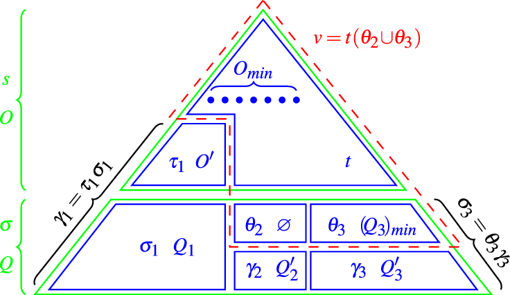
Figure 1. Proof of Lemma 27 with $P'\not=\varnothing$
.
$P'\not=\varnothing$
.
Q may contain positions that are minimal in P. Let $Q\!=\!Q_1\!\uplus\! Q_2\!\uplus\!Q_3$
, where
$Q\!=\!Q_1\!\uplus\! Q_2\!\uplus\!Q_3$
, where $Q_1\! >_{{\mathcal{P}}}\!(O\!\setminus\!O_{\rm min})_{\rm min}$
,
$Q_1\! >_{{\mathcal{P}}}\!(O\!\setminus\!O_{\rm min})_{\rm min}$
, $Q_2 >_{{\mathcal{P}}}O_{\rm min}\land Q_2\#(O\!\setminus\!O_{\rm min})_{\rm min}$
, and
$Q_2 >_{{\mathcal{P}}}O_{\rm min}\land Q_2\#(O\!\setminus\!O_{\rm min})_{\rm min}$
, and $Q_3\#O_{\rm min}$
. Note that
$Q_3\#O_{\rm min}$
. Note that $P_{\rm min}\!=\!O_{\rm min}\!\cup\!(Q_3)_{\rm min}$
. Since meta-variables must occur linearly in s, we split
$P_{\rm min}\!=\!O_{\rm min}\!\cup\!(Q_3)_{\rm min}$
. Since meta-variables must occur linearly in s, we split $\sigma$
as its restrictions
$\sigma$
as its restrictions $\sigma_1, \sigma_2$
, and
$\sigma_1, \sigma_2$
, and $\sigma_3$
to the meta-variables of s which occur above
$\sigma_3$
to the meta-variables of s which occur above $(Q_1)_{\rm min}$
,
$(Q_1)_{\rm min}$
, $(Q_2)_{\rm min}$
, and
$(Q_2)_{\rm min}$
, and $(Q_3)_{\rm min}$
, respectively. Using now successively Lemma 21 for
$(Q_3)_{\rm min}$
, respectively. Using now successively Lemma 21 for $\sigma_2$
and the induction hypothesis for
$\sigma_2$
and the induction hypothesis for $\sigma_3$
, we get
$\sigma_3$
, we get $\sigma_2 \displaystyle \mathop{\otimes\!\!\!\Longrightarrow}^{\varnothing\otimes_{\theta_2} Q'_2}_{i} \theta'_2\gamma'_2=\sigma'_2$
, with
$\sigma_2 \displaystyle \mathop{\otimes\!\!\!\Longrightarrow}^{\varnothing\otimes_{\theta_2} Q'_2}_{i} \theta'_2\gamma'_2=\sigma'_2$
, with $\sigma_2=\theta_2\gamma_2$
(note that
$\sigma_2=\theta_2\gamma_2$
(note that $\theta'_2=\theta_2$
), and
$\theta'_2=\theta_2$
), and $\sigma_3\displaystyle \mathop{\otimes\!\!\!\Longrightarrow}^{(Q_3)_{\rm min}\otimes_{\theta_3} Q'_3}_{i}\theta'_3\gamma'_3\!=\!\sigma'_3$
, with
$\sigma_3\displaystyle \mathop{\otimes\!\!\!\Longrightarrow}^{(Q_3)_{\rm min}\otimes_{\theta_3} Q'_3}_{i}\theta'_3\gamma'_3\!=\!\sigma'_3$
, with $\sigma_3=\theta_3\gamma_3$
. We finally construct v and
$\sigma_3=\theta_3\gamma_3$
. We finally construct v and $\gamma$
, hence defining v’ and
$\gamma$
, hence defining v’ and $\gamma'$
. Let
$\gamma'$
. Let $v=t(\theta_2\cup\theta_3)$
,
$v=t(\theta_2\cup\theta_3)$
, $v'= t'(\theta'_2\cup\theta'_3)$
,
$v'= t'(\theta'_2\cup\theta'_3)$
, $\gamma= \tau_1\sigma_1 \cup \gamma_2\cup\gamma_3$
and
$\gamma= \tau_1\sigma_1 \cup \gamma_2\cup\gamma_3$
and $\gamma'= \tau'_1\sigma'_1 \cup \gamma'_2\cup\gamma'_3$
. Let now
$\gamma'= \tau'_1\sigma'_1 \cup \gamma'_2\cup\gamma'_3$
. Let now $P'\!=\!O'\otimes_{\tau_1}Q_1 \!\cup\! Q'_2\!\cup\! Q'_3$
. Using associativity and stability, we get
$P'\!=\!O'\otimes_{\tau_1}Q_1 \!\cup\! Q'_2\!\cup\! Q'_3$
. Using associativity and stability, we get $u\displaystyle \mathop{\otimes\!\!\!\Longrightarrow}^{P_{\rm min}\otimes_{v}P'}_{i}\!v'\gamma'\!=\!u'$
.
$u\displaystyle \mathop{\otimes\!\!\!\Longrightarrow}^{P_{\rm min}\otimes_{v}P'}_{i}\!v'\gamma'\!=\!u'$
.
An important direct consequence of canonical splitting is that the outcome of an orthogonal rewrite step is entirely determined by its input term and set of orthogonal positions:
Lemma 28 (Functionality)
Let $P\otimes_K Q=P'\otimes_{K'} Q'$
,
$P\otimes_K Q=P'\otimes_{K'} Q'$
, $u\displaystyle \mathop{\otimes\!\!\!\Longrightarrow}^{P\otimes_K Q}_{i}v$
and
$u\displaystyle \mathop{\otimes\!\!\!\Longrightarrow}^{P\otimes_K Q}_{i}v$
and $u\displaystyle \mathop{\otimes\!\!\!\Longrightarrow}^{P'\otimes_{K'} Q'}_{i}v'$
. Then
$u\displaystyle \mathop{\otimes\!\!\!\Longrightarrow}^{P'\otimes_{K'} Q'}_{i}v'$
. Then $v=v'$
.
$v=v'$
.
The product notation has shown itself to be very convenient: we will use it systematically, in particular when P is empty, writing then $s\sigma\displaystyle \mathop{\otimes\!\!\!\Longrightarrow}^{\varnothing\otimes_s Q}_{i}s\tau$
, or when Q is empty, writing
$s\sigma\displaystyle \mathop{\otimes\!\!\!\Longrightarrow}^{\varnothing\otimes_s Q}_{i}s\tau$
, or when Q is empty, writing $s\sigma\displaystyle \mathop{\otimes\!\!\!\Longrightarrow}^{P\otimes_s\varnothing}_{i} t\sigma$
. It will serve as a type-checking device to control complex rewriting calculations.
$s\sigma\displaystyle \mathop{\otimes\!\!\!\Longrightarrow}^{P\otimes_s\varnothing}_{i} t\sigma$
. It will serve as a type-checking device to control complex rewriting calculations.
3.6 Critical peaks
Since patterns are $\beta$
-normal and left-linear, a
$\beta$
-normal and left-linear, a $\beta$
-redex cannot overlap a
$\beta$
-redex cannot overlap a ${\mathcal{R}}$
-redex at a position above its fringe. No wonder here, this is the only purpose of the assumption that patterns are
${\mathcal{R}}$
-redex at a position above its fringe. No wonder here, this is the only purpose of the assumption that patterns are $\beta$
-normal. Further,
$\beta$
-normal. Further, $\beta$
-redexes cannot overlap themselves either, except trivially.
$\beta$
-redexes cannot overlap themselves either, except trivially.
We are therefore interested in overlaps between the rules of ${\mathcal{R}}$
only, throughout the four coming sub-sections which deal successively with the definition of critical peaks, their calculation, their main property, and an example.
${\mathcal{R}}$
only, throughout the four coming sub-sections which deal successively with the definition of critical peaks, their calculation, their main property, and an example.
Our formulation of the definition of orthogonal rewriting has one main purpose: ease the definition of critical pairs and the proof of the associated critical peak property. Generating the minimal nested critical peaks that characterize the confluence of orthogonal rewriting requires computing the overlaps of two orthogonal rewriting steps issuing from a term. Such peaks are defined by two different rules, each left-hand side overlapping alternatively on the other at a set of parallel positions, but not between themselves so that there are two different orthogonal steps issuing from the same term. These overlaps form both horizontal chains when one left-hand side overlaps the other at several parallel positions, and vertical chains when there is an alternation of overlaps between the two left-hand sides.
As usual, overlapping a left-hand side of rule G at a subterm of another $L|_o$
frees the variables of
$L|_o$
frees the variables of $L|_o$
that are bound in L above o. Then, the meta-variables of G need to depend upon those variables, which may require increasing their arity. This is done with an operation called lifting (Ferey and Jouannaud Reference Ferey and Jouannaud2019), introduced first in this context by Nipkow in a slightly different form (Nipkow Reference Nipkow1991).
$L|_o$
that are bound in L above o. Then, the meta-variables of G need to depend upon those variables, which may require increasing their arity. This is done with an operation called lifting (Ferey and Jouannaud Reference Ferey and Jouannaud2019), introduced first in this context by Nipkow in a slightly different form (Nipkow Reference Nipkow1991).
Definition 29. (Lifting)
Given a term L and a list $\overline{x}$
of pairwise different variables such that
$\overline{x}$
of pairwise different variables such that ${{\mathcal{V}}}ar({L})\cap\overline{x}=\varnothing$
, we call lifting of L with respect to
${{\mathcal{V}}}ar({L})\cap\overline{x}=\varnothing$
, we call lifting of L with respect to $\overline{x}$
, denoted by
$\overline{x}$
, denoted by $L\!\uparrow^{\overline{x}}$
, the term
$L\!\uparrow^{\overline{x}}$
, the term $L\sigma_L^{\overline{x}}$
, where
$L\sigma_L^{\overline{x}}$
, where $\sigma_L^{\overline{x}} = \{ Y \mapsto Y'[\overline{x}] : Y \in M{\mathcal{V}} ar(L), Y' \mbox{ fresh},|Y'| = |Y| + |\overline{x}|\}$
.
$\sigma_L^{\overline{x}} = \{ Y \mapsto Y'[\overline{x}] : Y \in M{\mathcal{V}} ar(L), Y' \mbox{ fresh},|Y'| = |Y| + |\overline{x}|\}$
.
Lifting increases by $\overline{x}$
the list of arguments of all meta-variables occurring in L, hence their arity by
$\overline{x}$
the list of arguments of all meta-variables occurring in L, hence their arity by $|\overline{x}|$
, requiring changing their names to fresh ones. Note that lifting preserves pre-patterns.
$|\overline{x}|$
, requiring changing their names to fresh ones. Note that lifting preserves pre-patterns.
Example 6. Lifting the left-hand side $L = ud(V,lk(X))$
of rule (ul) with respect to the variable x gives the term
$L = ud(V,lk(X))$
of rule (ul) with respect to the variable x gives the term $L\!\uparrow^{x} = ud(V'[x],lk(X'[x]))$
, using substitution
$L\!\uparrow^{x} = ud(V'[x],lk(X'[x]))$
, using substitution $\sigma_L^{x} = \{ V \mapsto V'[x], X \mapsto X'[x] \}$
.
$\sigma_L^{x} = \{ V \mapsto V'[x], X \mapsto X'[x] \}$
.
An important property of lifting is the following:
Lemma 30. Assume that $u\displaystyle{\mathop{\longrightarrow}^{p}_{L\rightarrow R}} v$
. Then
$u\displaystyle{\mathop{\longrightarrow}^{p}_{L\rightarrow R}} v$
. Then $u=u[L\!\uparrow^{\overline{x}}\theta]_p$
for some
$u=u[L\!\uparrow^{\overline{x}}\theta]_p$
for some $\theta$
such that
$\theta$
such that ${{\mathcal{R}}}an({{\theta}})\cap\overline{x}=\varnothing$
, where
${{\mathcal{R}}}an({{\theta}})\cap\overline{x}=\varnothing$
, where $\overline{x}$
is the vector of variables bound above p in u.
$\overline{x}$
is the vector of variables bound above p in u.
Proof. By definition of rewriting, $u|_p=L\sigma$
. Let
$u|_p=L\sigma$
. Let $L\!\uparrow^{\overline{x}}=L\tau_L^{\overline{x}}$
. We define the substitution
$L\!\uparrow^{\overline{x}}=L\tau_L^{\overline{x}}$
. We define the substitution $\theta$
such that
$\theta$
such that $X'\mapsto \lambda\overline{x}. v\in\theta$
iff
$X'\mapsto \lambda\overline{x}. v\in\theta$
iff $X\mapsto v\in\sigma$
, where X’ is the renaming of X. Since
$X\mapsto v\in\sigma$
, where X’ is the renaming of X. Since $\tau_L^{\overline{x}}\theta=\sigma$
,
$\tau_L^{\overline{x}}\theta=\sigma$
, $L\!\uparrow^{\overline{x}}\theta=L\sigma$
.
$L\!\uparrow^{\overline{x}}\theta=L\sigma$
. ![]()
Definition 31 (Nested overlaps)
Given two rules $k\!:\!L\rightarrow R$
and
$k\!:\!L\rightarrow R$
and $l\!:\!G\rightarrow D$
in
$l\!:\!G\rightarrow D$
in ${\mathcal{R}}$
, a substitution
${\mathcal{R}}$
, a substitution $\sigma$
and a pure term u such that
$\sigma$
and a pure term u such that $u=_\alpha L\sigma$
, two sets
$u=_\alpha L\sigma$
, two sets $P\!=\!\{p_0={\Lambda}\}\!\uplus\!\{p_i\}_{i\in I}$
and
$P\!=\!\{p_0={\Lambda}\}\!\uplus\!\{p_i\}_{i\in I}$
and $Q\!=\!\{q_j\}_{j\in J}$
of positions in
$Q\!=\!\{q_j\}_{j\in J}$
of positions in ${{\mathcal{F}}{\mathcal{P}}}os({u})$
, two sets
${{\mathcal{F}}{\mathcal{P}}}os({u})$
, two sets $\{V_i\}_{i\in I}$
and
$\{V_i\}_{i\in I}$
and $\{W_j\}_{j\in J}$
such that
$\{W_j\}_{j\in J}$
such that $V_i$
and
$V_i$
and $W_j$
are the lists of (pairwise different) variables bound in u from positions
$W_j$
are the lists of (pairwise different) variables bound in u from positions $p_i$
and
$p_i$
and $q_j$
, respectively, to the root, and two sets
$q_j$
, respectively, to the root, and two sets $\{L_i\}_{i\in I}$
and
$\{L_i\}_{i\in I}$
and $\{G_j\}_{j\in J}$
of renamings of L, G, respectively, that share no meta-variables between themselves nor with
$\{G_j\}_{j\in J}$
of renamings of L, G, respectively, that share no meta-variables between themselves nor with $L=L_0$
, then
$L=L_0$
, then $\langle u, k, P, l, Q, \sigma\rangle$
is a nested overlap of G onto L at positions P,Q iff:
$\langle u, k, P, l, Q, \sigma\rangle$
is a nested overlap of G onto L at positions P,Q iff:
-
(i)
$\sigma$
satisfies the equality
$\bigwedge_{i\in I}u|_{p_i}= L_i\!\uparrow^{V_i}\sigma \land \bigwedge_{j\in J} u|_{q_j}=G_j\!\uparrow^{W_j}\sigma$
; -
(ii)
$\forall j\;\exists i\;(q_j\in p_i\cdot{{\mathcal{F}}{\mathcal{P}}}os({L})))$
and
$\forall j'\neq j\;(q_{j'}\not\in q_{j}\cdot{{\mathcal{F}}{\mathcal{P}}}os({G}))$
; -
(iii)
$\forall i\neq 0\;\exists j$
$(p_i\in q_j\cdot{{\mathcal{F}}{\mathcal{P}}}os({G}))$
and
$\forall i\neq i'\;(p_{i'}\not\in p_i\cdot{{\mathcal{F}}{\mathcal{P}}}os({L}))$
.


The nested overlap is critical if $\sigma$
is a most general higher-order unifier.
$\sigma$
is a most general higher-order unifier.
The particular case of critical nested overlap for which $P=\{{\Lambda}\}$
and Q is empty is said to be trivial. The set of non-trivial critical nested overlaps of rule l onto rule k is denoted by
$P=\{{\Lambda}\}$
and Q is empty is said to be trivial. The set of non-trivial critical nested overlaps of rule l onto rule k is denoted by ${\mathcal{C}} no(k,l)$
.
${\mathcal{C}} no(k,l)$
.
The particular case of non-trivial critical nested overlap for which $P=\{{\Lambda}\}$
and Q is a singleton set is called a critical overlap. Its set is denoted by
$P=\{{\Lambda}\}$
and Q is a singleton set is called a critical overlap. Its set is denoted by ${\mathcal{C}} o(k,l)$
.
${\mathcal{C}} o(k,l)$
.
The particular case of non-trivial critical nested overlap for which $P=\{{\Lambda}\}$
and Q is a nonempty set of parallel positions is called a critical parallel overlap. Its set is denoted by
$P=\{{\Lambda}\}$
and Q is a nonempty set of parallel positions is called a critical parallel overlap. Its set is denoted by ${\mathcal{C}} po(k,l)$
.
${\mathcal{C}} po(k,l)$
.
The particular case of nested overlap for which $P\!\setminus\!{\Lambda}$
is a nonempty set of pairwise parallel positions and Q is a singleton is called a critical 1-nested overlap. Its set is denoted by
$P\!\setminus\!{\Lambda}$
is a nonempty set of pairwise parallel positions and Q is a singleton is called a critical 1-nested overlap. Its set is denoted by ${\mathcal{C}} 1no(k,l)$
.
${\mathcal{C}} 1no(k,l)$
.
Condition (i) does not make visible the fact that matching is not syntactic, but modulo ${{\beta^0}}$
instead, since
${{\beta^0}}$
instead, since ${{\beta^0}}$
-steps are buried inside the definition of substitution for pre-redexes. It says that
${{\beta^0}}$
-steps are buried inside the definition of substitution for pre-redexes. It says that $\sigma$
, hence
$\sigma$
, hence $L\sigma$
, is entirely defined by condition (i), and that the subterms of u at other positions in P are k-redexes, while those at positions in Q are l-redexes. It follows that
$L\sigma$
, is entirely defined by condition (i), and that the subterms of u at other positions in P are k-redexes, while those at positions in Q are l-redexes. It follows that $\sigma$
could be omitted from the tuple
$\sigma$
could be omitted from the tuple $\langle u, k, P, l, Q, \sigma\rangle$
. Condition (ii) says that l-redexes overlap an above k-redex but no other l-redex. Condition (iii) for k-redexes but the topmost one is similar. It follows that P,Q are both sets of orthogonal positions for rules k and l, respectively, a property that is of course expected.
$\langle u, k, P, l, Q, \sigma\rangle$
. Condition (ii) says that l-redexes overlap an above k-redex but no other l-redex. Condition (iii) for k-redexes but the topmost one is similar. It follows that P,Q are both sets of orthogonal positions for rules k and l, respectively, a property that is of course expected.
When P and Q are singleton sets, hence $P=\{{\Lambda}\}$
, u is a usual higher-order overlap between the two rules. In general, the positions
$P=\{{\Lambda}\}$
, u is a usual higher-order overlap between the two rules. In general, the positions $p_i$
and
$p_i$
and $q_j$
keep increasing because of conditions (ii, iii), and the sets
$q_j$
keep increasing because of conditions (ii, iii), and the sets $V_i$
and
$V_i$
and $W_j$
of bound variables keep increasing as well, requiring new fresh meta-variables for each copy of
$W_j$
of bound variables keep increasing as well, requiring new fresh meta-variables for each copy of $L_i$
and
$L_i$
and $G_j$
. This may occur in practice as shown at Example 7.
$G_j$
. This may occur in practice as shown at Example 7.
Trivial critical peaks are not local peaks, since the rewrite takes place on a single side. They are used to establish the base case of the induction showing that critical peaks can be computed.
One may wonder why we call these critical peaks nested rather than orthogonal. First, orthogonality refers explicitly to the absence of critical pairs, so an orthogonal critical pair would be kind of self-contradicting. Another reason is that there is a single rule left-hand side sitting at the top of a seed. Therefore, all redexes occurring in a seed are nested inside that left-hand side’s instance, whether they extend the seed construction vertically or horizontally.
Non-trivial nested critical overlaps give rise to critical local peaks:
Lemma 32. Given $\langle u,k,P,l,Q,\sigma\rangle\in{\mathcal{C}} no(k:L\rightarrow R,l:G \rightarrow D)$
, then
$\langle u,k,P,l,Q,\sigma\rangle\in{\mathcal{C}} no(k:L\rightarrow R,l:G \rightarrow D)$
, then $v\displaystyle \mathop{\Longleftarrow\!\!\!\otimes}^{P}_{k} u=L\sigma \displaystyle \mathop{\otimes\!\!\!\Longrightarrow}^{Q}_{l} w$
. The triple (v,u,w) is called a nested critical peak of rule l onto rule k at positions P,Q while the pair (v,w) is the corresponding nested critical pair.
$v\displaystyle \mathop{\Longleftarrow\!\!\!\otimes}^{P}_{k} u=L\sigma \displaystyle \mathop{\otimes\!\!\!\Longrightarrow}^{Q}_{l} w$
. The triple (v,u,w) is called a nested critical peak of rule l onto rule k at positions P,Q while the pair (v,w) is the corresponding nested critical pair.
Proof. By (i) $u|_{p_i}=L_i\!\uparrow^{V_i}\sigma$
, where
$u|_{p_i}=L_i\!\uparrow^{V_i}\sigma$
, where $L_i\!\uparrow^{V_i}$
is an instance of L by the definition of lifting. Since substitutions compose,
$L_i\!\uparrow^{V_i}$
is an instance of L by the definition of lifting. Since substitutions compose, $u|_{p_i}$
is a k-redex. Similarly,
$u|_{p_i}$
is a k-redex. Similarly, $u|_{q_i}$
is a l-redex. Therefore, P and Q are sets of orthogonal positions for rule (k) by (iii) and for rule (l) by (ii), respectively. The result follows then from the definition of orthogonal rewriting.
$u|_{q_i}$
is a l-redex. Therefore, P and Q are sets of orthogonal positions for rule (k) by (iii) and for rule (l) by (ii), respectively. The result follows then from the definition of orthogonal rewriting. ![]()
The proof shows that lifting substitutions must be applied to the right-hand sides of rules.
Note also that this whole section appears as a genuine generalization of the usual critical pair theory or parallel critical pair theory, apart from the calculation of critical pairs which comes next.
3.7 Calculation of nested overlaps
The previous definition of a nested overlap does not allow us to compute $\sigma$
, hence the critical nested overlaps, since the positions
$\sigma$
, hence the critical nested overlaps, since the positions $p_k$
and
$p_k$
and $q_l$
are positions in
$q_l$
are positions in $L\sigma$
,
$L\sigma$
, $\sigma$
being yet unknown. An algorithm computing these overlaps must therefore proceed by successive unifications, possibly alternating between the two left-hand sides. Computing these overlaps requires then some bookkeeping, both in terms of substitutions and overlapping positions, in order to avoid self-overlaps of L and G. This is achieved by the next definition:
$\sigma$
being yet unknown. An algorithm computing these overlaps must therefore proceed by successive unifications, possibly alternating between the two left-hand sides. Computing these overlaps requires then some bookkeeping, both in terms of substitutions and overlapping positions, in order to avoid self-overlaps of L and G. This is achieved by the next definition:
Definition 33. (Seeds)
Given two rules $k\!:\!L\rightarrow R, l\!:\!G\rightarrow D$
from
$k\!:\!L\rightarrow R, l\!:\!G\rightarrow D$
from ${{{\mathcal{R}}}}$
, the set
${{{\mathcal{R}}}}$
, the set $p{\mathcal{S}}_l^k$
of (k,l)-pre-seeds is the smallest set of tuples
$p{\mathcal{S}}_l^k$
of (k,l)-pre-seeds is the smallest set of tuples $(s,\sigma,P,Q)$
, where P and Q are lists of positions in
$(s,\sigma,P,Q)$
, where P and Q are lists of positions in ${{\mathcal{F}}{\mathcal{P}}}os({s\sigma})$
of L-redexes and G-redexes, respectively, such that
${{\mathcal{F}}{\mathcal{P}}}os({s\sigma})$
of L-redexes and G-redexes, respectively, such that
-
(i)
$p{\mathcal{S}}_l^k$
contains the trivial pre-seed
$\langle L,\varnothing, \{{\Lambda}\},\{\,\}\rangle$
; -
(ii)
$p{\mathcal{S}}_l^k$
is closed under nested overlapping: given
$\langle s, \sigma, P, Q\rangle\in p{\mathcal{S}}_l^k$
, two lists of parallel positions
$\{p_i\in{{\mathcal{F}}{\mathcal{P}}}os({s\sigma}) : p_i\geq_{{\mathcal{P}}} P\cdot F_L\}_{i\in I}$
and
$\{q_j\in{{\mathcal{F}}{\mathcal{P}}}os({s\sigma}) : q_j\geq_{{\mathcal{P}}} Q\cdot F_G {\mbox{ if } Q\neq\varnothing}\}_{j\in J}$
which are not both empty and whose elements are pairwise incomparable, renamings
$\{L_i\}_{i\in I}$
of L and
$\{G_j\}_{j\in J}$
of G such that
$\forall i,j$
,
${{\mathcal{V}}}ar({L_i})$
,
${{\mathcal{V}}}ar({G_j})$
, and
${{\mathcal{V}}}ar({s\sigma})$
are pairwise disjoint sets, and
$\tau$
a most general unifier of the equation
$\bigwedge_{i\in I} (s\sigma)|_{p_i}=L_i\!\uparrow^{V_i} \land \bigwedge_{j\in J}$
$(s\sigma)|_{q_j}=G_j\!\uparrow^{W_j}$
, where
$V_i$
and
$W_j$
denote the variables bound in
$s\sigma$
above
$p_i$
and
$q_j$
, respectively, the non-trivial pre-seed
$\langle s\sigma,\tau, P\cup\{p_i\}_{i\in I}, Q\cup\{q_j\}_{j\in J}\rangle$
belongs to
$p{\mathcal{S}}_l^k$
.


We call seed a triple $\langle u\tau,P,Q\rangle$
where
$\langle u\tau,P,Q\rangle$
where $\langle u,\tau,P,Q\rangle$
is a pre-seed. The term
$\langle u,\tau,P,Q\rangle$
is a pre-seed. The term $u\tau$
is the nested overlap, P contains the positions in
$u\tau$
is the nested overlap, P contains the positions in $u\tau$
of the k-redexes and Q those of the l-redexes. A seed is trivial if
$u\tau$
of the k-redexes and Q those of the l-redexes. A seed is trivial if $Q\!=\!\emptyset$
. The set of seeds is denoted by
$Q\!=\!\emptyset$
. The set of seeds is denoted by ${\mathcal{S}}_l^k$
.
${\mathcal{S}}_l^k$
.
In the recursive definition of pre-seeds, the overlapping substitution $\sigma$
obtained tells us where to overlap next, while the maximal positions in P and Q of these overlaps tell us where to not overlap L and G, respectively. In particular, the initial overlap is impossible with L, unless
$\sigma$
obtained tells us where to overlap next, while the maximal positions in P and Q of these overlaps tell us where to not overlap L and G, respectively. In particular, the initial overlap is impossible with L, unless $k\!=\!l$
, but is possible with G. Subsequent overlaps may involve both L and G.
$k\!=\!l$
, but is possible with G. Subsequent overlaps may involve both L and G.
Since L,G are left-linear, higher-order unification of a lifted copy of G with some subterm of L (or vice-versa) does not instantiate these terms beyond their boundaries. It follows that each redex instance of L (resp., G) must overlap some left-hand side G (resp., L) obtained at the previous run. This remark is a property of the definition when the rules are left-linear; building it in the definition is useless.
Alternating overlaps with L and with G would eliminate some redundancies to the price of storing the run parity in the tuple. In practice, however, that would of course be the natural strategy for computing them.
Example 7 (Rules lu and ul of the theory of global states)
These two rules, like their well-chosen names, overlap themselves ad libitum because the head function symbol of each left-hand side is heading a strict subterm of the other which will be part of the substitution when unifying the rules.
The computation is represented in Figure 2. The color red is used for the left-hand side of (ul), and therefore of its subterms, while blue is used for the left-hand side of (lu). We consider the case where ul stands at the top. We adopt a renaming schema based on the value of a counter used to index the meta-variables and bound variables of each rule in turn. The starting value of the counter, used to index the meta-variables of the left-hand side of rule standing at the top, is zero. The initial rule (ul) is therefore $ud(V_0,lk(Y_0))\rightarrow ud(V_0, Y_0[V_0])$
. Each time a new equation is used, the counter is increased by one. So, the first use of rule (lu) is
$ud(V_0,lk(Y_0))\rightarrow ud(V_0, Y_0[V_0])$
. Each time a new equation is used, the counter is increased by one. So, the first use of rule (lu) is $lk(\lambda v_1.ud(v_1,X_1[v_1]))\rightarrow lk(X_1)$
. Overlapping positions appear then on the tree in violet, with a bullet in the exponent of the function symbol. The first overlap takes place at position 2. Note that both rules are represented in the figure; that’s why the first occurrence of lk has one blue successor with a blue link, and one red successor with a red link. The equation generated is therefore
$lk(\lambda v_1.ud(v_1,X_1[v_1]))\rightarrow lk(X_1)$
. Overlapping positions appear then on the tree in violet, with a bullet in the exponent of the function symbol. The first overlap takes place at position 2. Note that both rules are represented in the figure; that’s why the first occurrence of lk has one blue successor with a blue link, and one red successor with a red link. The equation generated is therefore ${lk(Y_0)}= {lk(\lambda v_1.ud(v_1, X_1[v_1]))}$
. It is displayed on the figure to the right of the first overlapping position. The substitution obtained from this equation is figured as an equality between a pre-redex and its value under the substitution. For
${lk(Y_0)}= {lk(\lambda v_1.ud(v_1, X_1[v_1]))}$
. It is displayed on the figure to the right of the first overlapping position. The substitution obtained from this equation is figured as an equality between a pre-redex and its value under the substitution. For ${Y_0}$
, we get
${Y_0}$
, we get ${\lambda v_1. ud(v_1,X_1[v_1]})={Y_0}$
. This value will of course change when new overlaps will take place successively, until the whole tree of Figure 2 is obtained. We have again fully represented the two rules and the equation generated from the second overlap at position
${\lambda v_1. ud(v_1,X_1[v_1]})={Y_0}$
. This value will of course change when new overlaps will take place successively, until the whole tree of Figure 2 is obtained. We have again fully represented the two rules and the equation generated from the second overlap at position $2\!\cdot\! 1\!\cdot\! 1$
.
$2\!\cdot\! 1\!\cdot\! 1$
.
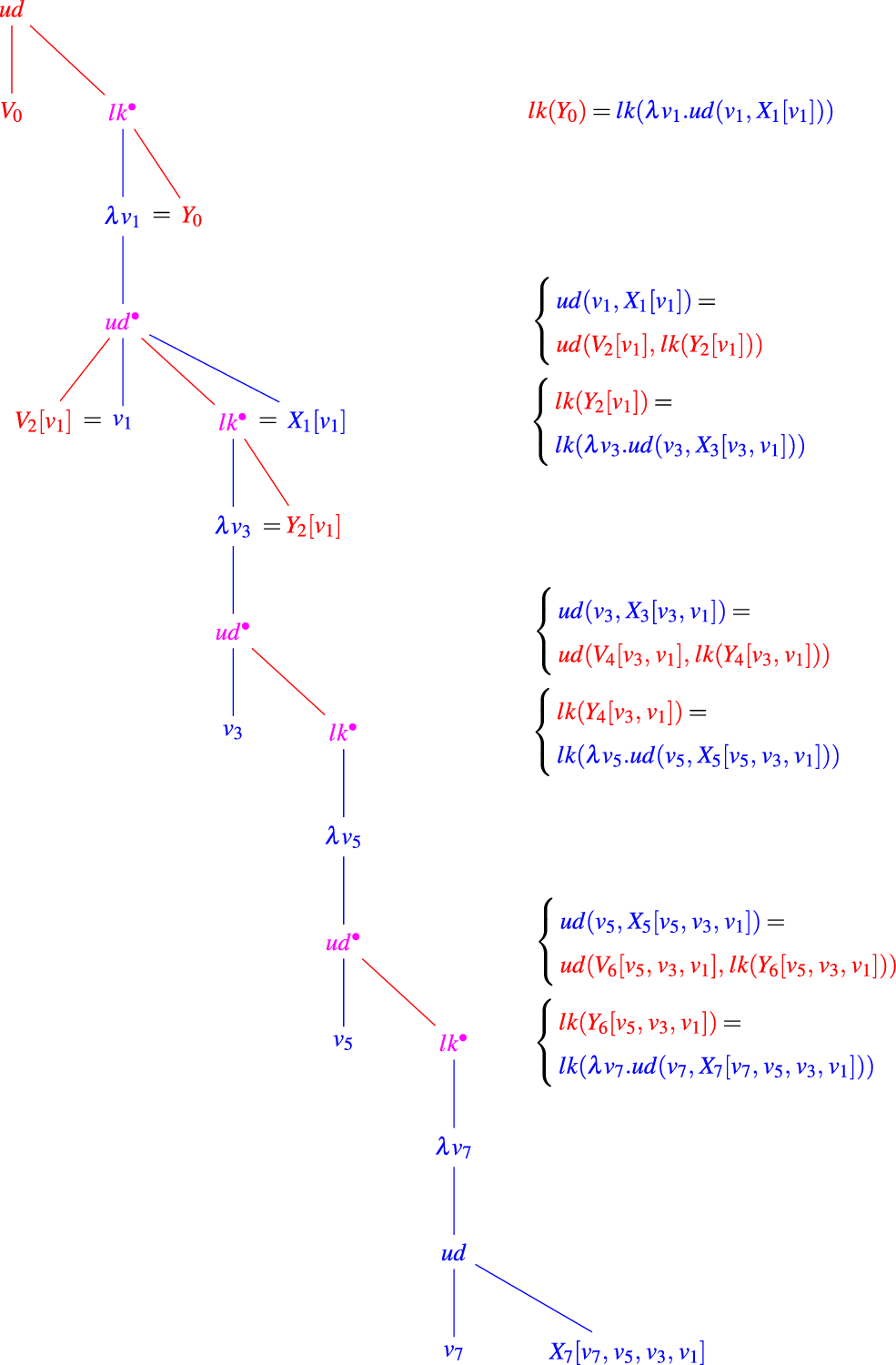
Figure 2. Computation of a nested overlap.
Let us now move to the seeds calculation. The initial pre-seed in $p{\mathcal{S}}^{ul}_{lu}$
is
$p{\mathcal{S}}^{ul}_{lu}$
is $\langle ud(V_0,lk(Y_0)), \varnothing, \{{\Lambda}\}, \{\}\rangle$
. The only possible overlap with ul requires
$\langle ud(V_0,lk(Y_0)), \varnothing, \{{\Lambda}\}, \{\}\rangle$
. The only possible overlap with ul requires $Q_1\!=\!\{2\}$
, a position above the fringe of
$Q_1\!=\!\{2\}$
, a position above the fringe of $ud(V_0,lk(Y_0))$
, and requires no lifting since there is no abstraction above position 2 in
$ud(V_0,lk(Y_0))$
, and requires no lifting since there is no abstraction above position 2 in $ud(V_0,lk(Y_0))$
. The equation obtained is displayed on the figure. Unification yields
$ud(V_0,lk(Y_0))$
. The equation obtained is displayed on the figure. Unification yields $Y_0=\lambda v_1.ud(v_1,X_1[v_1])$
, hence
$Y_0=\lambda v_1.ud(v_1,X_1[v_1])$
, hence $(ud(V_0,lk(\lambda v_1. X_1[v_1])), \{Y_0\mapsto\lambda v_1.ud(v_1,X_1[v_1])\}, \{{\Lambda}\}, \{2\})$
is added to
$(ud(V_0,lk(\lambda v_1. X_1[v_1])), \{Y_0\mapsto\lambda v_1.ud(v_1,X_1[v_1])\}, \{{\Lambda}\}, \{2\})$
is added to $p{\mathcal{S}}^{ul}_{lu}$
, and the computation proceeds with
$p{\mathcal{S}}^{ul}_{lu}$
, and the computation proceeds with $ud(V_0,lk(\lambda v_1. ud(v_1,X_1[v_1])$
, whith a unique possible overlapping position
$ud(V_0,lk(\lambda v_1. ud(v_1,X_1[v_1])$
, whith a unique possible overlapping position $2\cdot 1\cdot 1$
, which generates the equation
$2\cdot 1\cdot 1$
, which generates the equation ${ud(v_1,X_1[v_1])}= {ud(V_2[v_1],lk(Y_2[v_1]))}$
, whose solutions appear on the figure.
${ud(v_1,X_1[v_1])}= {ud(V_2[v_1],lk(Y_2[v_1]))}$
, whose solutions appear on the figure.
Following the picture, the reader can now easily continue the computation.
We finally get four infinite families of seeds, depending upon which left-hand side of rule stands at the top, and which one stands at the bottom. On the figure, (ul) stands at the top and (lu) at the bottom. Here are the four infinite families, where $\overline{v}$
denotes the list
$\overline{v}$
denotes the list $(v_{2n+1}, v_{2n-1},\ldots, v_1)$
, successively, (ul)
$(v_{2n+1}, v_{2n-1},\ldots, v_1)$
, successively, (ul) $\cdots$
(lu), (ul)
$\cdots$
(lu), (ul) $\cdots$
(ul), (lu)
$\cdots$
(ul), (lu) $\cdots$
(lu) and finally (lu)
$\cdots$
(lu) and finally (lu) $\cdots$
(ul):
$\cdots$
(ul):

The seed represented in the figure belongs to the second set. In all these nested overlaps, the set of sets of overlapping positions of (ul), or of (lu), is actually a set of singleton sets of overlapping positions. We have therefore identified both sets without ambiguity with sets of positions. Note also that our counter for indexing the variables and meta-variables is initialized by 0 for the first two seeds, and to 1 for the last two. This explains that we could use the same vector $\overline{v}$
of bound variables for all four seeds and that the last two nested overlappings are subterms of the first two.
$\overline{v}$
of bound variables for all four seeds and that the last two nested overlappings are subterms of the first two.
We now show that the sets of seeds and of critical nested overlappings are one-to-one (up to variable renaming of bound variables). This statement includes trivial critical nested overlappings and trivial seeds in order to facilitate its proof.
Theorem 34. Let R be a higher-order rewriting system such that $k,l\in R$
. Then,
$k,l\in R$
. Then, $\langle s, k, P, l, Q, \sigma\rangle\in{\mathcal{C}} no(l,k) \mbox{ iff }\langle s,P,Q\rangle\in{\mathcal{S}}_l^k$
.
$\langle s, k, P, l, Q, \sigma\rangle\in{\mathcal{C}} no(l,k) \mbox{ iff }\langle s,P,Q\rangle\in{\mathcal{S}}_l^k$
.
Of course, membership should be understood modulo the renaming of bound variables and meta-variables.
Proof. Note first that trivial critical nested overlappings and trivial seeds correspond.
-
•
${\mathcal{S}}_l^k\subseteq {\mathcal{C}} no(l,k)$
. It suffices to show that
${\mathcal{C}} no(l,k)$
is “closed under nested overlapping”. By definition of pre-seeds, let
$\langle s,\sigma, P, Q\rangle\in p{\mathcal{S}}_l^k$
,
$\{p_i\}_i$
and
$\{q_j\}_j$
be sets of positions,
$\{L_i\}_i$
and
$\{G_j\}_j$
be renamings of L,G, and
$\tau$
a substitution satisfying the condition (ii) of Definition 33. Using the induction hypothesis and the above conditions (ii), it is easy to verify that
$\langle s\sigma, k, P, l, Q, \sigma\rangle\in {\mathcal{C}} no(l,k)$
. -
•
${\mathcal{C}} no(l,k) \subseteq {\mathcal{S}}_l^k$
, the converse statement. Let
$\langle s, \sigma, k, P, l, Q\rangle\in p{\mathcal{C}} no(l,k)$
, and consider the sets P’,Q’ of positions in P,Q which are maximal in
$P\cup Q$
. Let
$P\setminus P'=\{p_i\}_i$
and
$Q\setminus Q'=\{q_j\}_j$
. By condition (i) and the fact that
$\sigma$
is minimal,
$\sigma=\theta\tau$
and
$s=t\tau$
, where
$\theta$
is the most general unifier of the equation
$t\!=\!L\theta\land \bigwedge_{i}u|_{p_i}= L_i\!\uparrow^{V_i}\theta \land \bigwedge_{j} u|_{q_j}=G_j\!\uparrow^{W_i}\theta$
. By conditions (ii, iii),
$\langle t, \theta, k, P\setminus P', l, Q\setminus Q'\rangle\in p{\mathcal{C}} no(l,k)$
is a critical nested overlapping. By induction hypothesis,
$\langle t,\theta, P, Q\rangle\in{\mathcal{S}}_l^k$
. By condition (i) and closure under nested overlappings
$\langle t,\tau, P, Q\rangle\in p{\mathcal{S}}_l^k$
, hence
$\langle t\tau=s, P, Q\rangle\in {\mathcal{S}}_l^k$
and we are done.


We could of course define the critical pairs themselves recursively in the same way we have defined the nested overlaps in Definition 33. It is, however, equivalent to rewrite the overlaps with the appropriate lifting of the right-hand sides of rules, which means that each rule needs to be lifted with lifting substitutions, implying that each rule needs infinitely many lifted copies in general.
3.8 Critical peak property
We conclude our study of orthogonal rewriting with the nested critical peak (or critical pair) property:
Theorem 35 (Nested Critical Peak)
Let $s\displaystyle \mathop{\Longleftarrow\!\!\!\otimes}^{\{{\Lambda}\}\cup P}_{k:L\rightarrow R} r \displaystyle \mathop{\otimes\!\!\!\Longrightarrow}^{Q}_{l:G\rightarrow D} t$
with
$s\displaystyle \mathop{\Longleftarrow\!\!\!\otimes}^{\{{\Lambda}\}\cup P}_{k:L\rightarrow R} r \displaystyle \mathop{\otimes\!\!\!\Longrightarrow}^{Q}_{l:G\rightarrow D} t$
with $Q\cap{{\mathcal{F}}{\mathcal{P}}}os({L})\!\neq\!\varnothing$
. Then,
$Q\cap{{\mathcal{F}}{\mathcal{P}}}os({L})\!\neq\!\varnothing$
. Then, $\exists u, v, w, u', v', w'$
,
$\exists u, v, w, u', v', w'$
, $\theta,\sigma, \tau, \gamma, O,O',$
P’, Q’ st:
$\theta,\sigma, \tau, \gamma, O,O',$
P’, Q’ st:
-
(i)
$r\!=\!u\theta, s\!=\!v\sigma, t\!=\!w\tau, u\!=\!u'\gamma, v\!=\!v'\gamma, w\!=\!w'\gamma$
, -
(ii)
$v'\displaystyle \mathop{\Longleftarrow\!\!\!\otimes}^{O}_{k} u' \displaystyle \mathop{\otimes\!\!\!\Longrightarrow}^{O'}_{l} w'$
$is\, a\, nested\, critical\, peak,$
-
(iii)
$\theta$
$is\, a\, substitution\, st$
$\sigma\displaystyle \mathop{\Longleftarrow\!\!\!\otimes}^{P'}_{k}\theta\displaystyle \mathop{\otimes\!\!\!\Longrightarrow}^{Q'}_{l}\tau$
, -
(iv)
$P\!=\!O\otimes_u P'$
and
$Q\!=\!O'\otimes_u Q'$
.


This statement is pictured in Figure 3. The substitution $\theta$
is obtained by splitting r as
$\theta$
is obtained by splitting r as $u\theta$
so that u contains a critical overlap. The substitution
$u\theta$
so that u contains a critical overlap. The substitution $\gamma$
expresses the property that u is an instance of the most general critical peak (v’, u’, w’), hence
$\gamma$
expresses the property that u is an instance of the most general critical peak (v’, u’, w’), hence $u\!=\! u'\gamma$
. These substitutions play different rÔles, the substitution
$u\!=\! u'\gamma$
. These substitutions play different rÔles, the substitution $\theta$
is rewritten while the substitution
$\theta$
is rewritten while the substitution $\gamma$
is not, that is why they are kept separate.
$\gamma$
is not, that is why they are kept separate.
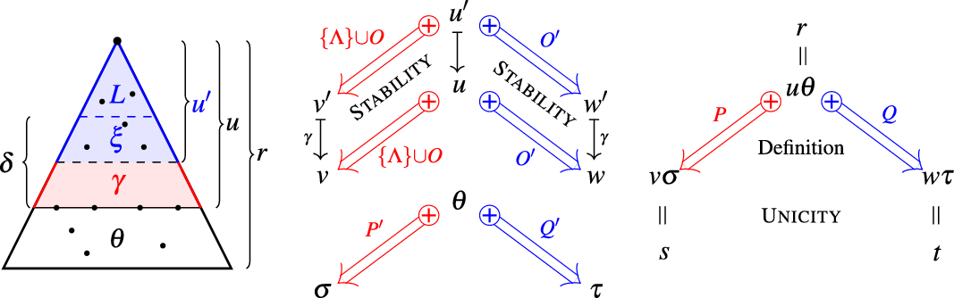
Figure 3. Nested critical peak property.
Proof. By assumption on Q, the two orthogonal rewrites from r overlap. Let $O\!=\!\{O_i\}_{i\in I}$
and
$O\!=\!\{O_i\}_{i\in I}$
and $O'\!=\!\{O'_j\}_{j\in J}$
be the maximal subsets of P and Q, respectively, that satisfy conditions (ii, iii) of Definition 31. Let now
$O'\!=\!\{O'_j\}_{j\in J}$
be the maximal subsets of P and Q, respectively, that satisfy conditions (ii, iii) of Definition 31. Let now $N=((P\!\cup\! Q)\!\setminus\!(O\!\cup\! O'))_{\rm min}$
,
$N=((P\!\cup\! Q)\!\setminus\!(O\!\cup\! O'))_{\rm min}$
, $u=\underline{r}_{N}$
and
$u=\underline{r}_{N}$
and $\theta=\overline{r}^{N}$
, hence
$\theta=\overline{r}^{N}$
, hence $r=u\theta$
.
$r=u\theta$
.
We first show that there exists a substitution $\delta$
such that the tuple
$\delta$
such that the tuple $\langle u,k, \{{\Lambda}\}\cup O, l, O',\delta\rangle$
is a nested overlap, hence satisfies condition (i) of the same definition. Since
$\langle u,k, \{{\Lambda}\}\cup O, l, O',\delta\rangle$
is a nested overlap, hence satisfies condition (i) of the same definition. Since $\{{\Lambda}\}\cup P$
and Q are sets of orthogonal positions, so are their respective subsets
$\{{\Lambda}\}\cup P$
and Q are sets of orthogonal positions, so are their respective subsets $\{{\Lambda}\}\cup O$
and O’. By definition of orthogonal rewriting and maximality of O,O’, the positions
$\{{\Lambda}\}\cup O$
and O’. By definition of orthogonal rewriting and maximality of O,O’, the positions $n\!\in\! N$
do not belong to any set of the form
$n\!\in\! N$
do not belong to any set of the form $p\cdot\{o<_{{\mathcal{P}}} F_L\cup F_G\}$
for some p and o, unless
$p\cdot\{o<_{{\mathcal{P}}} F_L\cup F_G\}$
for some p and o, unless $p = n$
, or
$p = n$
, or $q\cdot\{o<_{{\mathcal{P}}} F_L\cup F_G\}$
for some q and o, unless
$q\cdot\{o<_{{\mathcal{P}}} F_L\cup F_G\}$
for some q and o, unless $q = n$
. Hence,
$q = n$
. Hence, $\{{\Lambda}\}\cup O$
and O’ are sets of orthogonal positions in u, and therefore, by linearity of L and G, the terms in
$\{{\Lambda}\}\cup O$
and O’ are sets of orthogonal positions in u, and therefore, by linearity of L and G, the terms in $\{u|_p: p\in \{{\Lambda}\}\cup O\}$
are k-redexes while the terms
$\{u|_p: p\in \{{\Lambda}\}\cup O\}$
are k-redexes while the terms $\{u|_q\in O'\}$
are l-redexes, hence are instances of L and G, respectively. Let
$\{u|_q\in O'\}$
are l-redexes, hence are instances of L and G, respectively. Let $O=\{o_i\}_{i\in I}$
and
$O=\{o_i\}_{i\in I}$
and $O'=\{o'_j\}_{j\in J}$
,
$O'=\{o'_j\}_{j\in J}$
, $\{L_i\}_{i\in I}$
and
$\{L_i\}_{i\in I}$
and $\{G_j\}_{j\in J}$
be renamings of L and G, respectively, that share no meta-variable between themselves nor with L. Then,
$\{G_j\}_{j\in J}$
be renamings of L and G, respectively, that share no meta-variable between themselves nor with L. Then, $u=L\sigma$
,
$u=L\sigma$
, $u|_{p_i}=L_i\sigma_i$
and
$u|_{p_i}=L_i\sigma_i$
and $u|_j=G_j\tau_j$
. By Lemma 30,
$u|_j=G_j\tau_j$
. By Lemma 30, $u|_{p_i}=L_i\!\uparrow^{V_i}\delta_i$
, where
$u|_{p_i}=L_i\!\uparrow^{V_i}\delta_i$
, where $\overline{V_i}$
is the vector of variables bound above
$\overline{V_i}$
is the vector of variables bound above $p_i$
in u, hence in r, and
$p_i$
in u, hence in r, and $u|_{q_j}=G_j\!\uparrow^{W_j}\delta_j$
, where
$u|_{q_j}=G_j\!\uparrow^{W_j}\delta_j$
, where $\overline{W_i}$
is the vector of variables bound above
$\overline{W_i}$
is the vector of variables bound above $q_j$
in u’, hence in r. Note that lifting is used here to ensure that the free variables coincide in u,
$q_j$
in u’, hence in r. Note that lifting is used here to ensure that the free variables coincide in u, $L\delta$
(there are no free variables),
$L\delta$
(there are no free variables), $L_i\!\uparrow^{V_i}\delta_i$
(whose set of free variables is
$L_i\!\uparrow^{V_i}\delta_i$
(whose set of free variables is $V_i$
) and
$V_i$
) and $G_j\!\uparrow^{V_j}\delta_j$
(whose set of free variables is
$G_j\!\uparrow^{V_j}\delta_j$
(whose set of free variables is $W_j$
). Since the respective domains of these substitutions are pairwise disjoint, their union
$W_j$
). Since the respective domains of these substitutions are pairwise disjoint, their union $\delta$
satisfies condition (i).
$\delta$
satisfies condition (i).
We can now exhibit the critical nested overlap. Let $\xi$
be the most general substitution satisfying (i), hence
$\xi$
be the most general substitution satisfying (i), hence $\delta=\xi\gamma$
for some
$\delta=\xi\gamma$
for some $\gamma$
,
$\gamma$
, $u'=L\xi$
and
$u'=L\xi$
and $u=u'\gamma$
. Then
$u=u'\gamma$
. Then $\langle u',k, \{{\Lambda}\}\!\cup\!O, l, O',\xi\rangle$
is a critical nested overlap. By Lemma 32,
$\langle u',k, \{{\Lambda}\}\!\cup\!O, l, O',\xi\rangle$
is a critical nested overlap. By Lemma 32, $s'\displaystyle \mathop{\Longleftarrow\!\!\!\otimes}^{\{{\Lambda}\}\cup O}_{k} u' \displaystyle \mathop{\otimes\!\!\!\Longrightarrow}^{O'}_{l} t'$
for some s’,t’. Hence,
$s'\displaystyle \mathop{\Longleftarrow\!\!\!\otimes}^{\{{\Lambda}\}\cup O}_{k} u' \displaystyle \mathop{\otimes\!\!\!\Longrightarrow}^{O'}_{l} t'$
for some s’,t’. Hence, $v=s'\gamma\displaystyle \mathop{\Longleftarrow\!\!\!\otimes}^{\{{\Lambda}\}\cup O}_{k} u=u'\gamma \displaystyle \mathop{\otimes\!\!\!\Longrightarrow}^{O'}_{l} t\gamma'=w$
by stability.
$v=s'\gamma\displaystyle \mathop{\Longleftarrow\!\!\!\otimes}^{\{{\Lambda}\}\cup O}_{k} u=u'\gamma \displaystyle \mathop{\otimes\!\!\!\Longrightarrow}^{O'}_{l} t\gamma'=w$
by stability.
Consider now the left-over rewrites applying to the substitution $\theta$
. By Lemma 14,
$\theta$
. By Lemma 14, $P\!=O\!\otimes_N\! P'$
and
$P\!=O\!\otimes_N\! P'$
and $Q\!=\!O'\!\otimes_N\! Q'$
. Since P and Q are sets of orthogonal positions for r, P’ and Q’, their respective subsets below N, are sets of orthogonal positions for
$Q\!=\!O'\!\otimes_N\! Q'$
. Since P and Q are sets of orthogonal positions for r, P’ and Q’, their respective subsets below N, are sets of orthogonal positions for $\theta$
. Hence,
$\theta$
. Hence, $\sigma\displaystyle \mathop{\Longleftarrow\!\!\!\otimes}^{P'}_{i} \theta\displaystyle \mathop{\otimes\!\!\!\Longrightarrow}^{Q'}_{j} \tau$
by Lemma 32.
$\sigma\displaystyle \mathop{\Longleftarrow\!\!\!\otimes}^{P'}_{i} \theta\displaystyle \mathop{\otimes\!\!\!\Longrightarrow}^{Q'}_{j} \tau$
by Lemma 32.
We have got two local orthogonal peaks, one from u and one from $\theta$
, that can be merged by definition of orthogonal rewriting. Since
$\theta$
, that can be merged by definition of orthogonal rewriting. Since $P=(\{{\Lambda}\}\cup O)\otimes_u P'$
and
$P=(\{{\Lambda}\}\cup O)\otimes_u P'$
and $Q=O'\otimes_u Q'$
, we get the peak
$Q=O'\otimes_u Q'$
, we get the peak $v\sigma\displaystyle \mathop{\Longleftarrow\!\!\!\otimes}^{P}_{k} u\theta\displaystyle \mathop{\otimes\!\!\!\Longrightarrow}^{Q}_{l} w\tau$
. Since
$v\sigma\displaystyle \mathop{\Longleftarrow\!\!\!\otimes}^{P}_{k} u\theta\displaystyle \mathop{\otimes\!\!\!\Longrightarrow}^{Q}_{l} w\tau$
. Since $r=u\gamma$
, we finally conclude that
$r=u\gamma$
, we finally conclude that $s=v\sigma$
and
$s=v\sigma$
and $t=w\tau$
by Lemma 28.
$t=w\tau$
by Lemma 28. ![]()
Of course, this result has particular cases: one-nested critical overlaps give rise to one-nested critical peaks (or critical pairs), parallel critical overlaps give rise to parallel critical peaks (or critical pairs), and critical overlaps give rise to critical peaks (or critical pairs). The latter case is sometimes dubbed plain to distinguish it from the others.
3.9 Nested critical pairs of the theory of global states
Using our example of global states, we illustrate the computation of two nested critical peaks and of one of the infinite families of nested critical peaks.


And now, the first infinite family of seeds described in Example 7:

4. Confluence in
${{\lambda{\mathcal{F}}}}$

Our goal here is to state and prove our main result, namely, the Church–Rosser property for a rewrite theory in ${{\lambda{\mathcal{F}}}}$
, under the assumption that its nested critical peaks have decreasing diagrams.
${{\lambda{\mathcal{F}}}}$
, under the assumption that its nested critical peaks have decreasing diagrams.
Since beta-reductions do not terminate on untyped terms, and higher-order reductions may be non-terminating as well, we shall use van Oostrom’s technique relying on the existence of a decreasing rewrite diagram for each local peak (van Oostrom Reference van Oostrom1994), decreasingness being defined wrt a partial quasi-order $\unrhd$
labeling the rewrite steps whose strict part
$\unrhd$
labeling the rewrite steps whose strict part $\rhd$
must be well-founded.
$\rhd$
must be well-founded.
The structure of this section is as follows: first, we describe the rewrite relation we use for proving confluence, and the corresponding labeling schema; second, we recall the notion of decreasing diagram and state the confluence theorem; third, we apply the result to the theory of global states; fourth, we apply it to the theory of encoding and decoding; lastly, comes the proof of the result.
4.1 Labeled rewrites in
${{\lambda{\mathcal{F}}}}$

We now consider the Church–Rosser property of the rewrite relation used in ${{\lambda{\mathcal{F}}}}$
on untyped terms. As usual, it is essential to choose carefully the relation to work with. For the method to be sound, it must contain rewriting and define the same convertibility relation as the one generated by the set of rules. Higher-order rewriting will suffice for those rules that define a terminating rewrite relation. For those that do not, non-linearities make it difficult to get decreasing diagrams for ancestor peaks since there can only be one facing step on each side of the conversion. The way out is to impose left-linearity and use some form of parallel rewriting to handle non-right-linearities. But parallel higher-order rewrites taking place below a beta-step may now become both duplicated and nested, making orthogonal higher-order rewriting necessary to get decreasing diagrams. Functional steps will be considered as particular steps requiring the use of orthogonal rewriting.
${{\lambda{\mathcal{F}}}}$
on untyped terms. As usual, it is essential to choose carefully the relation to work with. For the method to be sound, it must contain rewriting and define the same convertibility relation as the one generated by the set of rules. Higher-order rewriting will suffice for those rules that define a terminating rewrite relation. For those that do not, non-linearities make it difficult to get decreasing diagrams for ancestor peaks since there can only be one facing step on each side of the conversion. The way out is to impose left-linearity and use some form of parallel rewriting to handle non-right-linearities. But parallel higher-order rewrites taking place below a beta-step may now become both duplicated and nested, making orthogonal higher-order rewriting necessary to get decreasing diagrams. Functional steps will be considered as particular steps requiring the use of orthogonal rewriting.
We now assume a subset ${\mathcal{S}}\subseteq{\mathcal{R}}$
of small rules defining a terminating relation on untyped terms. All other rules are big rules.
${\mathcal{S}}\subseteq{\mathcal{R}}$
of small rules defining a terminating relation on untyped terms. All other rules are big rules. $\beta$
-rewrite steps will be smallest among the big steps, so that they can be neglected when needed, while small steps will be smaller than big steps. The definition of
$\beta$
-rewrite steps will be smallest among the big steps, so that they can be neglected when needed, while small steps will be smaller than big steps. The definition of ${\mathcal{S}}$
will therefore result from a compromise between two constraints: termination which allows a rule to be small, and the possible need of
${\mathcal{S}}$
will therefore result from a compromise between two constraints: termination which allows a rule to be small, and the possible need of $\beta$
-rewrites to join its critical pairs, which may force it to be big. Note that functional steps cannot be smaller than small steps: if they were, ancestor peaks having a small step below a functional step could not be made decreasing.
$\beta$
-rewrites to join its critical pairs, which may force it to be big. Note that functional steps cannot be smaller than small steps: if they were, ancestor peaks having a small step below a functional step could not be made decreasing.
The rewrite steps to be considered in an arbitrary conversion, for which all local peaks must be replaced by decreasing diagrams, are therefore of one of the three following forms:
 \begin{equation*}=_\alpha,\quad\mathop{\longrightarrow}^{}_{{\mathcal{S}}} \quad\mbox{and}\quad \displaystyle \mathop{\otimes\!\!\!\Longrightarrow}^{}_{\beta\cup({\mathcal{R}}\setminus{\mathcal{S}})}\end{equation*}
For uniformity, we use the notation $u\displaystyle{\mathop{\longrightarrow}^{p}_{\alpha}}v$
for an
$u\displaystyle{\mathop{\longrightarrow}^{p}_{\alpha}}v$
for an $=_\alpha$
-step taking place in the subterm
$=_\alpha$
-step taking place in the subterm $u|_p$
. Furthermore, we sometimes allow ourselves to abbreviate a sequence
$u|_p$
. Furthermore, we sometimes allow ourselves to abbreviate a sequence $\displaystyle{\mathop{\longrightarrow}^{p_1}_{}}\ldots\displaystyle{\mathop{\longrightarrow}^{p_n}_{}}$
by
$\displaystyle{\mathop{\longrightarrow}^{p_1}_{}}\ldots\displaystyle{\mathop{\longrightarrow}^{p_n}_{}}$
by $\displaystyle{\mathop{\Longrightarrow}^{P}_{}}$
when
$\displaystyle{\mathop{\Longrightarrow}^{P}_{}}$
when $P=\{p_i\}_i$
is a set of parallel positions.
$P=\{p_i\}_i$
is a set of parallel positions.
Main assumptions:
-
•
${\mathcal{R}}$
is a set of rules whose left-hand sides are linear patterns; -
•
${\mathcal{S}}$
is a subset of rules of
${\mathcal{R}}$
, whose rewrite relation is terminating; -
•
$\unrhd$
is a quasi order on rule names whose strict part is well-founded and equivalence is
$\equiv$
; -
•
$\forall i\in{\mathcal{R}}\!\setminus\!{\mathcal{S}}\;\forall j,k\in{\mathcal{S}}:\;i\rhd \beta\rhd j\equiv k \rhd \alpha$
.


We now label a step $s\displaystyle{\mathop{\longrightarrow}^{p}_{i}}t$
or
$s\displaystyle{\mathop{\longrightarrow}^{p}_{i}}t$
or $s\displaystyle \mathop{\otimes\!\!\!\Longrightarrow}^{P}_{i}t$
by a pair of the following form:
$s\displaystyle \mathop{\otimes\!\!\!\Longrightarrow}^{P}_{i}t$
by a pair of the following form:
 \begin{equation*}I=\langle i, \_\rangle, \mbox{ where $\_$ is a dummy, if } i\not\in{\mathcal{S}};\quad I=\langle i, s\rangle, \mbox{ if $i\in{\mathcal{S}}$ }\end{equation*}
Labels are compared lexicographically: our quasi order on labels is therefore $(\unrhd, \displaystyle \mathop{\longrightarrow\!\!\!\!\!\!\!\longrightarrow}^{}_{{\mathcal{S}}})_{lex}$
.
$(\unrhd, \displaystyle \mathop{\longrightarrow\!\!\!\!\!\!\!\longrightarrow}^{}_{{\mathcal{S}}})_{lex}$
.
Since the main order is the one on rule names, we will take the liberty to use $\unrhd$
as our quasi-order on labels and on rule names at the same time. The reader will easily disambiguate when needed. The strict part of this order is well-founded by construction.
$\unrhd$
as our quasi-order on labels and on rule names at the same time. The reader will easily disambiguate when needed. The strict part of this order is well-founded by construction.
Because of its definition, the label of a rewrite step would not need to appear in our rewriting notation, unless in specific occasions where it will replace the rule name. In order to disambiguate between these two situations, we will use small letters for rule names, say i, and the corresponding capital letter I for a label whose first argument is the rule name i and the second some term s.
Key properties of the order on labels are monotonicity and stability, for which it will be convenient to define the following notation: given a context $u[\_]_p$
, a substitution
$u[\_]_p$
, a substitution $\sigma$
and a label
$\sigma$
and a label $I=\langle i, a\rangle$
,
$I=\langle i, a\rangle$
, $u[I]_p\sigma$
is the label
$u[I]_p\sigma$
is the label $\langle i, u[a]_p\sigma\rangle$
, where
$\langle i, u[a]_p\sigma\rangle$
, where $u[a]_p\sigma=\_$
if
$u[a]_p\sigma=\_$
if $a=\_$
and the term
$a=\_$
and the term $u[s]_p\sigma$
if a is the term s. The notation extends of course to the case where there are multiple holes in u, as in
$u[s]_p\sigma$
if a is the term s. The notation extends of course to the case where there are multiple holes in u, as in $u[\overline{I}]_P\sigma$
, all labels in
$u[\overline{I}]_P\sigma$
, all labels in $\overline{I}$
using rule i. This will be used later with P being the positions of the meta-variables of u.
$\overline{I}$
using rule i. This will be used later with P being the positions of the meta-variables of u.
Lemma 36 Let $K=\langle k,a\rangle$
and
$K=\langle k,a\rangle$
and $L=\langle l,b\rangle$
be the labels of two rewrite steps such that
$L=\langle l,b\rangle$
be the labels of two rewrite steps such that $K\rhd L$
,
$K\rhd L$
, $u[\_]_o$
a context, and
$u[\_]_o$
a context, and $\sigma$
a substitution. Then,
$\sigma$
a substitution. Then, $K'=u[K]_o\sigma \rhd u[L]_o\sigma=L'$
.
$K'=u[K]_o\sigma \rhd u[L]_o\sigma=L'$
.
Proof. If $k\rhd l$
, this is trivial. Otherwise,
$k\rhd l$
, this is trivial. Otherwise, $k\equiv l\in{\mathcal{S}}$
,
$k\equiv l\in{\mathcal{S}}$
, $a=u$
and
$a=u$
and $b=v$
for some terms u,v such that
$b=v$
for some terms u,v such that $u\displaystyle \mathop{\longrightarrow\!\!\!\!\!\!\!\longrightarrow}^{}_{{\mathcal{S}}}v$
. Hence,
$u\displaystyle \mathop{\longrightarrow\!\!\!\!\!\!\!\longrightarrow}^{}_{{\mathcal{S}}}v$
. Hence, $w[u]_o\sigma\displaystyle \mathop{\longrightarrow\!\!\!\!\!\!\!\longrightarrow}^{}_{{\mathcal{S}}}w[v]_o\sigma$
by monotonicity and stability of higher-order rewriting, and the result follows.
$w[u]_o\sigma\displaystyle \mathop{\longrightarrow\!\!\!\!\!\!\!\longrightarrow}^{}_{{\mathcal{S}}}w[v]_o\sigma$
by monotonicity and stability of higher-order rewriting, and the result follows. ![]()
4.2 The confluence theorem
van Oostrom’s decreasing diagrams can have a very general form. We shall, however, stick to a more convenient one for the confluence proof:
Definition 37. (DRDs) Given a pair of labels (I,J), a decreasing reduction (DR) from u to v wrt (I,J) is a reduction of the form $u\displaystyle \mathop{\longrightarrow\!\!\!\!\!\!\!\longrightarrow}^{}_{\overline{K}}s\displaystyle \mathop{\otimes\!\!\!\Longrightarrow}^{P}_{J} t \displaystyle \mathop{\longrightarrow\!\!\!\!\!\!\!\longrightarrow}^{}_{\overline{L}}v$
, where labels in
$u\displaystyle \mathop{\longrightarrow\!\!\!\!\!\!\!\longrightarrow}^{}_{\overline{K}}s\displaystyle \mathop{\otimes\!\!\!\Longrightarrow}^{P}_{J} t \displaystyle \mathop{\longrightarrow\!\!\!\!\!\!\!\longrightarrow}^{}_{\overline{L}}v$
, where labels in $\overline{K}$
labeling the side steps are strictly smaller than I and labels in
$\overline{K}$
labeling the side steps are strictly smaller than I and labels in $\overline{L}$
labeling the middle steps are strictly smaller than either I or J. A decreasing reduction whose facing step from s to t is empty (
$\overline{L}$
labeling the middle steps are strictly smaller than either I or J. A decreasing reduction whose facing step from s to t is empty ( $P=\varnothing$
) is called simple.
$P=\varnothing$
) is called simple.
We often leave the labels implicit, writing then $u\displaystyle \mathop{\longrightarrow\!\!\!\!\!\!\!\longrightarrow}^{}_{\lhd I} \displaystyle \mathop{\otimes\!\!\!\Longrightarrow}^{P}_{J} \displaystyle \mathop{\longrightarrow\!\!\!\!\!\!\!\longrightarrow}^{}_{\lhd I,J} v$
or
$u\displaystyle \mathop{\longrightarrow\!\!\!\!\!\!\!\longrightarrow}^{}_{\lhd I} \displaystyle \mathop{\otimes\!\!\!\Longrightarrow}^{P}_{J} \displaystyle \mathop{\longrightarrow\!\!\!\!\!\!\!\longrightarrow}^{}_{\lhd I,J} v$
or $u\displaystyle \mathop{\longrightarrow\!\!\!\!\!\!\!\longrightarrow}^{}_{\lhd I,J}v$
if
$u\displaystyle \mathop{\longrightarrow\!\!\!\!\!\!\!\longrightarrow}^{}_{\lhd I,J}v$
if $P=\varnothing$
.
$P=\varnothing$
.
Given a local peak $v \displaystyle \mathop{\Longleftarrow\!\!\!\otimes}^{P}_{I} u \displaystyle \mathop{\otimes\!\!\!\Longrightarrow}^{Q}_{J}w$
, a decreasing rewrite diagram (DRD) is a pair of decreasing reductions from v to v’ wrt (I,J) and from w to w’ wrt (J,I), such that
$v \displaystyle \mathop{\Longleftarrow\!\!\!\otimes}^{P}_{I} u \displaystyle \mathop{\otimes\!\!\!\Longrightarrow}^{Q}_{J}w$
, a decreasing rewrite diagram (DRD) is a pair of decreasing reductions from v to v’ wrt (I,J) and from w to w’ wrt (J,I), such that $v'=_{M\eta} w'$
.
$v'=_{M\eta} w'$
.
Note that any joinability diagram $\displaystyle \mathop{\longrightarrow\!\!\!\!\!\!\!\longrightarrow}^{}_{{\mathcal{S}}} =_{M\eta} \displaystyle \mathop{\longleftarrow\!\!\!\!\!\!\!\longleftarrow}^{}_{\,{\mathcal{S}}}$
using small rules is indeed a decreasing rewrite diagram whose decreasing reductions are simple since small rules are terminating. There are other situations where decreasing reductions become simple. If
$\displaystyle \mathop{\longrightarrow\!\!\!\!\!\!\!\longrightarrow}^{}_{{\mathcal{S}}} =_{M\eta} \displaystyle \mathop{\longleftarrow\!\!\!\!\!\!\!\longleftarrow}^{}_{\,{\mathcal{S}}}$
using small rules is indeed a decreasing rewrite diagram whose decreasing reductions are simple since small rules are terminating. There are other situations where decreasing reductions become simple. If $i\in{\mathcal{R}}\setminus{\mathcal{S}}$
and
$i\in{\mathcal{R}}\setminus{\mathcal{S}}$
and $j\in{\mathcal{S}}$
, then any decreasing reduction with respect to (I,J) reduces to a simple decreasing reduction of the form
$j\in{\mathcal{S}}$
, then any decreasing reduction with respect to (I,J) reduces to a simple decreasing reduction of the form $u\displaystyle \mathop{\longrightarrow\!\!\!\!\!\!\!\longrightarrow}^{}_{\lhd I,J}$
, since
$u\displaystyle \mathop{\longrightarrow\!\!\!\!\!\!\!\longrightarrow}^{}_{\lhd I,J}$
, since $\displaystyle \mathop{\otimes\!\!\!\Longrightarrow}^{P}_{J}$
expands to
$\displaystyle \mathop{\otimes\!\!\!\Longrightarrow}^{P}_{J}$
expands to $\displaystyle \mathop{\longrightarrow\!\!\!\!\!\!\!\longrightarrow}^{}_{j}$
by Lemma 25, hence all steps in the sequence are strictly smaller than I. Two other cases are the following:
$\displaystyle \mathop{\longrightarrow\!\!\!\!\!\!\!\longrightarrow}^{}_{j}$
by Lemma 25, hence all steps in the sequence are strictly smaller than I. Two other cases are the following: $i=\beta$
and
$i=\beta$
and $j\in{\mathcal{S}}$
; and
$j\in{\mathcal{S}}$
; and $i\in{\mathcal{R}}\setminus {\mathcal{S}}$
and
$i\in{\mathcal{R}}\setminus {\mathcal{S}}$
and $j=\beta$
.
$j=\beta$
.
Our formulation of decreasing reductions includes $\alpha$
-steps in both sequences
$\alpha$
-steps in both sequences $\overline{K}$
and
$\overline{K}$
and $\overline{L}$
, that is why they do not need to appear explicitly at the bottom. On the other hand,
$\overline{L}$
, that is why they do not need to appear explicitly at the bottom. On the other hand, $\eta$
-expansions (or reductions) for meta-variables need to appear only at the bottom since they are absorbed by matching in decreasing reductions. These expansions can be ignored since they vanish by taking instantiations (Lemma 2). We will only find them in decreasing diagrams for critical pairs.
$\eta$
-expansions (or reductions) for meta-variables need to appear only at the bottom since they are absorbed by matching in decreasing reductions. These expansions can be ignored since they vanish by taking instantiations (Lemma 2). We will only find them in decreasing diagrams for critical pairs.
There is a single orthogonal step in a decreasing reduction, the other steps being plain higher-order rewrite steps. The reason is that any orthogonal step whose label is strictly less than I or J in a decreasing reduction wrt (I,J) can be expanded into a rewrite derivation by Lemma 25, decreasingness being then preserved. On the other hand, it is in general not possible to expand the orthogonal j-step without violating the decreasing diagram condition: there may be at most one (facing) step labeled by J. Collecting many j-steps into a single orthogonal j-step is the very reason for introducing orthogonal rewriting.
DRDs have better properties than arbitrary decreasing diagrams that ease the confluence proof in many (nonessential) ways. In practice, searching for DRDs is easier than searching for arbitrary decreasing diagrams; this is another reason for considering them.
We can now state the main result of the paper:
Theorem 38. A left-linear rewrite theory $({\mathcal{F}}, {\mathcal{R}})$
such that
$({\mathcal{F}}, {\mathcal{R}})$
such that ${\mathcal{R}}$
contains a subset of terminating confluent rules
${\mathcal{R}}$
contains a subset of terminating confluent rules ${\mathcal{S}}$
is confluent on closed terms if all the following conditions hold:
${\mathcal{S}}$
is confluent on closed terms if all the following conditions hold:
-
• the non-trivial nested critical peaks of
${\mathcal{R}}\!\setminus\!{\mathcal{S}}$
have rewrite diagrams decreasing wrt rule labeling; -
• the non-trivial plain critical pairs of
${\mathcal{S}}$
are joinable; -
• the parallel critical overlaps of
${\mathcal{R}}\setminus{\mathcal{S}}$
onto
${\mathcal{S}}$
not at the root have rewrite diagrams decreasing wrt rule labeling composed lexicographically with small rules rewriting; -
• the plain critical peaks and one-nested critical peaks of
${\mathcal{S}}$
onto
${\mathcal{R}}\setminus{\mathcal{S}}$
have rewrite diagrams decreasing wrt rule labeling composed lexicographically with small rules rewriting.


Of course, some nested critical peaks of ${\mathcal{R}}\setminus{\mathcal{S}}$
may be one-nested critical peaks, or parallel critical peaks, or even plain critical peaks.
${\mathcal{R}}\setminus{\mathcal{S}}$
may be one-nested critical peaks, or parallel critical peaks, or even plain critical peaks.
Before developing the proof that spans over Section 4.5, we illustrate its use with two examples, the first having infinitely many nested critical peaks, and the second requiring $\beta$
-steps to join some plain critical peaks.
$\beta$
-steps to join some plain critical peaks.
4.3 Confluence of the theory of global states
We illustrate now the confluence theorem with our example of global states. After recalling the rules, come the critical pairs computations presented inside individual boxes, the nested critical pairs that happen to be usual critical pairs first, then those that generate infinite families. For the case of usual critical pairs, in the upper middle of each box appear two rules whose superposition is inside braces. The upper rule is displayed in red, the lower one in blue with the proviso that lifted variables appear in red inside a blue rule. Next comes the unifier, then the colored right-hand sides, then the reduced right-hand sides, and finally the decreasing diagram part itself. Colored rule names label the arrows issuing from the critical overlap. The decreasing reductions are in black, including the rule names, except for the facing steps which are in red or blue (remember that simple reductions cannot contain a facing step). The presentation is a bit different, but still very similar, for the infinite families.
Let us first recall the rules:

As shown in (Ferey and Jouannaud Reference Ferey and Jouannaud2019), these rules do not terminate, which is why their confluence was proved there for a subset of the whole set of terms, namely by assuming that the first argument of ud belongs to a set of constant symbols (meant to correspond to the semantic values). We do not make such an assumption here, but use instead the easy to prove property that the subset ${\mathcal{S}}=\{uu,ll\}$
of linear rules defines a terminating rewrite relation, hence can be used as our set of small rules. Showing its confluence is done below by showing that its critical pairs are joinable (Knuth and Bendix Reference Knuth and Bendix1970), which we do now. The overlap of the first rule upon itself is just a usual first-order overlap. The second, however, requires lifting since the overlapping position is below an abstraction.
${\mathcal{S}}=\{uu,ll\}$
of linear rules defines a terminating rewrite relation, hence can be used as our set of small rules. Showing its confluence is done below by showing that its critical pairs are joinable (Knuth and Bendix Reference Knuth and Bendix1970), which we do now. The overlap of the first rule upon itself is just a usual first-order overlap. The second, however, requires lifting since the overlapping position is below an abstraction.


We now proceed with the computation, and checking of the critical pairs originating from overlapping a big rule at an internal position of one of the small rules.


We continue with the checking of 1-nested critical pairs originating from an overlapping of a small rule at a position of one of the big rules. All of them happen indeed to be critical pairs. Note that the next critical pair obtained by overlapping (l) with (ll) requires the use of the Drop unification rule (Ferey and Jouannaud Reference Ferey and Jouannaud2019), which generates a fresh meta-variable Z of arity one, in order to eliminate the dependency of $X_1$
upon its second argument w:
$X_1$
upon its second argument w:


We are left with the nested critical pairs between big rules. As we have seen, there are four infinite families of critical overlaps between ul and lu that we have computed already at Example 7. Since each family contains infinitely many critical pairs, we have to show that they all enjoy a decreasing rewrite diagram.


We have therefore shown that the theory of global states preserves the confluence of $\beta$
-reductions on all untyped terms, hence improving over (Ferey and Jouannaud Reference Ferey and Jouannaud2019), by using the order on rules’ labels inherited from the decision to have ll and uu as small rules. This example could actually not be shown confluent with an empty set of small rules, as can be checked by the reader, because, in that case, there would be additional infinite families whose joinability diagram would require
$\beta$
-reductions on all untyped terms, hence improving over (Ferey and Jouannaud Reference Ferey and Jouannaud2019), by using the order on rules’ labels inherited from the decision to have ll and uu as small rules. This example could actually not be shown confluent with an empty set of small rules, as can be checked by the reader, because, in that case, there would be additional infinite families whose joinability diagram would require $\{uu,ll\}\rhd \{ul, lu\}$
to be decreasing, while the existing infinite families require just the contrary.
$\{uu,ll\}\rhd \{ul, lu\}$
to be decreasing, while the existing infinite families require just the contrary.
An important remark here is that the checking of nested critical pairs, whether automatic or by the user for the infinite families of nested pairs, proceeds by accumulating ordering constraints on the rules’ names used for labeling the rewrite steps, and checking them for satisfiability, usually by rewriting the constraint into some disjunctive normal form. As is well-known, such a technique is modular: when new rules come in, new nested critical pairs are computed and new constraints added to the previous normal form, then the whole set gets normalized again and satisfiability or unsatisfiability concluded.
4.4 Confluence of encoding and decoding
We illustrate now the confluence theorem with our example of encoding and decoding terms, and show that all its nested critical pairs have decreasing diagrams. Just as with the previous example, we first recall the rules before computing and checking first the nested critical pairs that happen to be usual critical pairs, and then those that generate infinite families.
Let us first recall the rules:

The subset of rules $\{de,el,dl,ae,ad\}$
can be seen as a set of first-order rules,
$\{de,el,dl,ae,ad\}$
can be seen as a set of first-order rules, $\lambda x$
being a unary operator and bound occurrences of x in the scope of
$\lambda x$
being a unary operator and bound occurrences of x in the scope of $\lambda x$
being constants, since no meta-variable is applied in the right-hand side of the rules. We show that the rules are strongly normalizing by using the following (non-erasing) polynomial interpretation over
$\lambda x$
being constants, since no meta-variable is applied in the right-hand side of the rules. We show that the rules are strongly normalizing by using the following (non-erasing) polynomial interpretation over $\mathbb{N}^+$
:
$\mathbb{N}^+$
:
 \begin{equation*}\begin{array}{rcl|rcl}{{[\!\!\mid \!\! {\;\lambda x.t\; } \!\! \mid\!\!]}} &= & {{[\!\!\mid \!\! {\;t\; } \!\! \mid\!\!]}}+1 &\qquad {{[\!\!\mid \!\! {\;\mathsf{\Lambda}(t)\; } \!\! \mid\!\!]}} &= & {{[\!\!\mid \!\! {\;t\; } \!\! \mid\!\!]}} \\{{[\!\!\mid \!\! {\;(u~v)\; } \!\! \mid\!\!]}} = {{[\!\!\mid \!\! {\;@(u,v)\; } \!\! \mid\!\!]}} &= & {{[\!\!\mid \!\! {\;u\; } \!\! \mid\!\!]}}^2({{[\!\!\mid \!\! {\;v\; } \!\! \mid\!\!]}}+1) \qquad &{{[\!\!\mid \!\! {\;x\; } \!\! \mid\!\!]}} &= & 1 \\{{[\!\!\mid \!\! {\;\mathsf{\Downarrow}(t)\; } \!\! \mid\!\!]}} = {{[\!\!\mid \!\! {\;\mathsf{\Uparrow}(t)\; } \!\! \mid\!\!]}} &= & 2{{[\!\!\mid \!\! {\;t\; } \!\! \mid\!\!]}}+1\end{array}\end{equation*}
We now prove that this interpretation decreases strictly each rule. The check is trivial for de, el and dl. For ae, we need to verify that
 \begin{equation*}(2X+1)^2(Y+1)= 4X^2Y + 4XY + 4X + Y +1 > 2(X^2(2Y+1+1))+1= 4X^2Y + 4XY + 1\end{equation*}
which holds true. Naturally, neither al nor $\beta$
decrease this interpretation since either of these rules is non-terminating on its own.
$\beta$
decrease this interpretation since either of these rules is non-terminating on its own.
Choosing all these five rules as small rules would actually not work: two critical peaks require using $\beta$
-rewrites in their joining diagrams, which prevents us from keeping el and ad among the small rules. The set of small rules is therefore reduced to
$\beta$
-rewrites in their joining diagrams, which prevents us from keeping el and ad among the small rules. The set of small rules is therefore reduced to $\{de,ae,dl\}$
. The remaining rules are then ordered as follows:
$\{de,ae,dl\}$
. The remaining rules are then ordered as follows: $\{el,ad\}\rhd al \rhd \beta$
. There are then no nested critical pair, no one-nested critical pair, and four critical pairs that we consider in turn:
$\{el,ad\}\rhd al \rhd \beta$
. There are then no nested critical pair, no one-nested critical pair, and four critical pairs that we consider in turn:


Note here that using multi-step instead of orthogonal rewriting would produce one more critical pair, actually a one-nested critical pair obtained by overlapping (de) onto (ad) and (el) onto (de). This would correspond to a multi-step using both (ad) and (el) connected by a rewrite step using (dl). Thanks to our definition of orthogonal rewriting, this extra critical pair does not need to be considered.
We conclude that the encoding and decoding specification defines a confluent system together with $\beta$
.
$\beta$
.
4.5 The confluence proof
Using the generalization of van Oostrom’s theorem by Jouannaud and Liu (Jouannaud and Liu Reference Jouannaud and Liu2012), we need to show the existence of decreasing diagrams for all local peaks in turn. We develop first some properties of decreasing reductions.
4.5.1 Properties of decreasing reductions
Lemma 39 (Stability and monotonicity)
Let $I=\langle i,a\rangle$
,
$I=\langle i,a\rangle$
, $J=\langle j,b\rangle$
be labels,
$J=\langle j,b\rangle$
be labels, $s\displaystyle \mathop{\longrightarrow\!\!\!\!\!\!\!\longrightarrow}^{}_{\overline{K}} \displaystyle \mathop{\otimes\!\!\!\Longrightarrow}^{P}_{i}\displaystyle \mathop{\longrightarrow\!\!\!\!\!\!\!\longrightarrow}^{}_{\overline{L}}t$
a decreasing derivation with respect to (I,J),
$s\displaystyle \mathop{\longrightarrow\!\!\!\!\!\!\!\longrightarrow}^{}_{\overline{K}} \displaystyle \mathop{\otimes\!\!\!\Longrightarrow}^{P}_{i}\displaystyle \mathop{\longrightarrow\!\!\!\!\!\!\!\longrightarrow}^{}_{\overline{L}}t$
a decreasing derivation with respect to (I,J), $u[]_p$
a context and
$u[]_p$
a context and $\sigma$
a substitution. Then
$\sigma$
a substitution. Then $u[s\sigma]_p\displaystyle \mathop{\longrightarrow\!\!\!\!\!\!\!\longrightarrow}^{}_{\overline{K'}}\displaystyle \mathop{\otimes\!\!\!\Longrightarrow}^{}_{i}\displaystyle \mathop{\longrightarrow\!\!\!\!\!\!\!\longrightarrow}^{}_{\overline{L'}} u[t\sigma]_p$
is a decreasing derivation with respect to
$u[s\sigma]_p\displaystyle \mathop{\longrightarrow\!\!\!\!\!\!\!\longrightarrow}^{}_{\overline{K'}}\displaystyle \mathop{\otimes\!\!\!\Longrightarrow}^{}_{i}\displaystyle \mathop{\longrightarrow\!\!\!\!\!\!\!\longrightarrow}^{}_{\overline{L'}} u[t\sigma]_p$
is a decreasing derivation with respect to $\langle u[I]_p\sigma, u[J]_p\sigma\rangle$
.
$\langle u[I]_p\sigma, u[J]_p\sigma\rangle$
.
Proof. By Lemma 36. ![]()
We will actually need a more general form of monotonicity for orthogonal reductions, for which the linear context u has multiple holes defined as the positions of the meta-variables in ${{\mathcal{D}}}om({{\sigma}})$
. The proof is by induction on the number of meta-variables in u.
${{\mathcal{D}}}om({{\sigma}})$
. The proof is by induction on the number of meta-variables in u.
Lemma 40. (Multi-monotonicity)
Given a linear term u whose meta-variable X occurs at a set P of parallel positions, a substitution $\sigma$
of domain
$\sigma$
of domain $M{\mathcal{V}} ar(u)$
, and labels
$M{\mathcal{V}} ar(u)$
, and labels $I=\langle i,a\rangle$
and
$I=\langle i,a\rangle$
and $J=\langle j,b\rangle$
such that
$J=\langle j,b\rangle$
such that $\sigma(X)\displaystyle \mathop{\longrightarrow\!\!\!\!\!\!\!\longrightarrow}^{}_{I\lhd Ia} \displaystyle \mathop{\otimes\!\!\!\Longrightarrow}^{}_{i}\displaystyle \mathop{\longrightarrow\!\!\!\!\!\!\!\longrightarrow}^{}_{J\lhd Ia,Ib}\tau(X)$
a decreasing reductions wrt
$\sigma(X)\displaystyle \mathop{\longrightarrow\!\!\!\!\!\!\!\longrightarrow}^{}_{I\lhd Ia} \displaystyle \mathop{\otimes\!\!\!\Longrightarrow}^{}_{i}\displaystyle \mathop{\longrightarrow\!\!\!\!\!\!\!\longrightarrow}^{}_{J\lhd Ia,Ib}\tau(X)$
a decreasing reductions wrt $\langle I_a, J_b\rangle$
, then,
$\langle I_a, J_b\rangle$
, then, $u\sigma\displaystyle \mathop{\longrightarrow\!\!\!\!\!\!\!\longrightarrow}^{}_{I'}\displaystyle \mathop{\otimes\!\!\!\Longrightarrow}^{}_{i}\displaystyle \mathop{\longrightarrow\!\!\!\!\!\!\!\longrightarrow}^{}_{J'} u\tau$
is a decreasing reduction wrt
$u\sigma\displaystyle \mathop{\longrightarrow\!\!\!\!\!\!\!\longrightarrow}^{}_{I'}\displaystyle \mathop{\otimes\!\!\!\Longrightarrow}^{}_{i}\displaystyle \mathop{\longrightarrow\!\!\!\!\!\!\!\longrightarrow}^{}_{J'} u\tau$
is a decreasing reduction wrt $\langle u[I]_{P}\sigma, u[J]_{P}\sigma\rangle$
.
$\langle u[I]_{P}\sigma, u[J]_{P}\sigma\rangle$
.
Proof. By Lemma 39 applied repeatedly to $X\sigma$
for s instantiated by the identity substitution.
$X\sigma$
for s instantiated by the identity substitution. ![]()
We now consider gluing together two decreasing reductions.
Lemma 41 (Gluing)
Let $j\in({\mathcal{R}}\cup\beta)\setminus$
, and
$j\in({\mathcal{R}}\cup\beta)\setminus$
, and $u\displaystyle \mathop{\longrightarrow\!\!\!\!\!\!\!\longrightarrow}^{}_{\lhd I} u'\displaystyle \mathop{\otimes\!\!\!\Longrightarrow}^{P}_{j}v'\displaystyle \mathop{\longrightarrow\!\!\!\!\!\!\!\longrightarrow}^{}_{\lhd I,J}v$
and
$u\displaystyle \mathop{\longrightarrow\!\!\!\!\!\!\!\longrightarrow}^{}_{\lhd I} u'\displaystyle \mathop{\otimes\!\!\!\Longrightarrow}^{P}_{j}v'\displaystyle \mathop{\longrightarrow\!\!\!\!\!\!\!\longrightarrow}^{}_{\lhd I,J}v$
and $\sigma\displaystyle \mathop{\longrightarrow\!\!\!\!\!\!\!\longrightarrow}^{}_{\lhd I} \sigma'\displaystyle \mathop{\otimes\!\!\!\Longrightarrow}^{Q}_{j}\tau'\displaystyle \mathop{\longrightarrow\!\!\!\!\!\!\!\longrightarrow}^{}_{\lhd I,J}\tau$
be two decreasing derivations originating from a term u and a substitution
$\sigma\displaystyle \mathop{\longrightarrow\!\!\!\!\!\!\!\longrightarrow}^{}_{\lhd I} \sigma'\displaystyle \mathop{\otimes\!\!\!\Longrightarrow}^{Q}_{j}\tau'\displaystyle \mathop{\longrightarrow\!\!\!\!\!\!\!\longrightarrow}^{}_{\lhd I,J}\tau$
be two decreasing derivations originating from a term u and a substitution $\sigma$
, respectively.
$\sigma$
, respectively.
Then, $u\sigma \displaystyle \mathop{\longrightarrow\!\!\!\!\!\!\!\longrightarrow}^{}_{\lhd I}u'\sigma'\displaystyle \mathop{\otimes\!\!\!\Longrightarrow}^{P\otimes_{u'}Q}_{J} v'\tau'\displaystyle \mathop{\longrightarrow\!\!\!\!\!\!\!\longrightarrow}^{}_{\lhd I,J}v\tau$
is a decreasing derivation from
$u\sigma \displaystyle \mathop{\longrightarrow\!\!\!\!\!\!\!\longrightarrow}^{}_{\lhd I}u'\sigma'\displaystyle \mathop{\otimes\!\!\!\Longrightarrow}^{P\otimes_{u'}Q}_{J} v'\tau'\displaystyle \mathop{\longrightarrow\!\!\!\!\!\!\!\longrightarrow}^{}_{\lhd I,J}v\tau$
is a decreasing derivation from $u\sigma$
to
$u\sigma$
to $v\tau$
wrt (I,J).
$v\tau$
wrt (I,J).
Proof. Follows from stability properties of reductions as above, from their monotonicity properties, and from the definition of orthogonal reductions. ![]()
4.5.2 Decreasing diagrams for free
Before starting to build decreasing diagrams for all local peaks, we need to generalize some standard commutation properties of plain rewriting to the case of higher-order orthogonal reductions. These algebraic properties of reductions can be seen as decreasing diagrams for free. They will of course play an important rÔle in the confluence proof.
Plain first-order rewriting enjoys two properties implying that disjoint and ancestor local rewriting peaks are always joinable by decreasing reductions, called disjoint peak (DP) property and linear ancestor peak (LAP) property for left-linear rewrite rules (Huet Reference Huet1980). (DP) is true of all monotonic relations, and (LAP) holds for our definition of higher-order rewriting as we have seen. It is important to realize that our definition of higher-order rewriting has been designed with this objective in mind: neither (DP) nor (LAP) are true of Nipkow’s definition. As expected, these properties extend to orthogonal higher-order rewrites:
Lemma 42 (DP) Let $Q\# P$
be sets of orthogonal positions wrt rule i. Then, orthogonal i-rewrite steps at P and Q commute.
$Q\# P$
be sets of orthogonal positions wrt rule i. Then, orthogonal i-rewrite steps at P and Q commute.
Note that P (resp., Q) are singleton sets when rewriting takes place at a single position.
Lemma 43 (Commutation)
Let $j\in{{{\mathcal{R}}}}\cup\beta$
. Then,
$j\in{{{\mathcal{R}}}}\cup\beta$
. Then, $\displaystyle{\mathop{\longleftarrow}^{p}_{\alpha}}\;\displaystyle \mathop{\otimes\!\!\!\Longrightarrow}^{Q}_{j} \subseteq\displaystyle \mathop{\otimes\!\!\!\Longrightarrow}^{Q}_{j}\; \displaystyle \mathop{\longleftarrow\!\!\!\!\!\!\!\longleftarrow}^{}_{\,\alpha}$
.
$\displaystyle{\mathop{\longleftarrow}^{p}_{\alpha}}\;\displaystyle \mathop{\otimes\!\!\!\Longrightarrow}^{Q}_{j} \subseteq\displaystyle \mathop{\otimes\!\!\!\Longrightarrow}^{Q}_{j}\; \displaystyle \mathop{\longleftarrow\!\!\!\!\!\!\!\longleftarrow}^{}_{\,\alpha}$
.
This straightforward property is required in the case where a rewrite relation is modulo a theory, here modulo $=_\alpha$
(Jouannaud and Liu Reference Jouannaud and Liu2012).
$=_\alpha$
(Jouannaud and Liu Reference Jouannaud and Liu2012).
Lemma 44 (LAPo)
Let $i:L\rightarrow R, j:G\rightarrow D\in{{{\mathcal{R}}}}\cup\beta$
, u a term such that
$i:L\rightarrow R, j:G\rightarrow D\in{{{\mathcal{R}}}}\cup\beta$
, u a term such that $u\displaystyle{\mathop{\longrightarrow}^{p}_{i}}v$
and
$u\displaystyle{\mathop{\longrightarrow}^{p}_{i}}v$
and $\sigma$
a substitution such that
$\sigma$
a substitution such that $\sigma(X)\displaystyle \mathop{\otimes\!\!\!\Longrightarrow}^{Q_X}_{j}\tau(X)$
for each meta-variable X in
$\sigma(X)\displaystyle \mathop{\otimes\!\!\!\Longrightarrow}^{Q_X}_{j}\tau(X)$
for each meta-variable X in ${{\mathcal{D}}}om({{\sigma}})$
. Let
${{\mathcal{D}}}om({{\sigma}})$
. Let $Q=\{Q_X\}_{X\in{{\mathcal{D}}}om({{\sigma}})}$
. Then,
$Q=\{Q_X\}_{X\in{{\mathcal{D}}}om({{\sigma}})}$
. Then, $v\sigma\displaystyle{\mathop{\longleftarrow}^{p}_{i}} u\sigma\displaystyle \mathop{\otimes\!\!\!\Longrightarrow}^{\varnothing\otimes_u Q}_{j}u\tau$
and
$v\sigma\displaystyle{\mathop{\longleftarrow}^{p}_{i}} u\sigma\displaystyle \mathop{\otimes\!\!\!\Longrightarrow}^{\varnothing\otimes_u Q}_{j}u\tau$
and $v\sigma\displaystyle \mathop{\otimes\!\!\!\Longrightarrow}^{\varnothing\otimes_v Q}_{j} v\tau\displaystyle{\mathop{\longleftarrow}^{p}_{i}}u\tau$
.
$v\sigma\displaystyle \mathop{\otimes\!\!\!\Longrightarrow}^{\varnothing\otimes_v Q}_{j} v\tau\displaystyle{\mathop{\longleftarrow}^{p}_{i}}u\tau$
.
In the case where $j\in{\mathcal{S}}$
, the orthogonal step from
$j\in{\mathcal{S}}$
, the orthogonal step from $\sigma(X)$
to
$\sigma(X)$
to $\tau(X)$
is indeed a plain rewrite step since small rules use plain rewriting instead of orthogonal rewriting, but seen here as an orthogonal step at the singleton set
$\tau(X)$
is indeed a plain rewrite step since small rules use plain rewriting instead of orthogonal rewriting, but seen here as an orthogonal step at the singleton set $Q_X$
, while the orthogonal steps in the conclusion become parallel steps. This allows us to avoid writing specific lemmas for the case of small rules.
$Q_X$
, while the orthogonal steps in the conclusion become parallel steps. This allows us to avoid writing specific lemmas for the case of small rules.
Proof. By stability Lemma 9 for the step from $u\tau$
to
$u\tau$
to $v\tau$
and by definition of orthogonal rewriting for the step from
$v\tau$
and by definition of orthogonal rewriting for the step from $v\sigma$
to
$v\sigma$
to $v\tau$
.
$v\tau$
. ![]()
4.5.3 Decreasing diagrams for arbitrary higher-order local peaks
This is the difficult case of local peaks, whose proof is based on using Theorem 35. It also requires lifting decreasing reductions from critical peaks to overlapping peaks, as well as gluing together decreasing derivations obtained for a term and its substitution. We do not distinguish here ancestor peaks from overlapping peaks, a typology that is not necessary for the case of orthogonal rewriting. Nor do we distinguish the kind of rule that is used, functional, small, or big.
Lemma 45. Higher-order local orthogonal peaks have decreasing diagrams provided higher-order nested critical peaks have decreasing rewrite diagrams.
Of course nested critical peaks between small rules are just usual critical peaks, while those between small and big rules are either usual critical peaks or 1-nested critical peaks if the big rule applies above (non-strictly) the small rule.
Proof. Let $v\displaystyle \mathop{\Longleftarrow\!\!\!\otimes}^{P}_{I} u \displaystyle \mathop{\otimes\!\!\!\Longrightarrow}^{Q}_{J} w$
be an orthogonal higher-order local peak with
$v\displaystyle \mathop{\Longleftarrow\!\!\!\otimes}^{P}_{I} u \displaystyle \mathop{\otimes\!\!\!\Longrightarrow}^{Q}_{J} w$
be an orthogonal higher-order local peak with $i,j\in{\mathcal{R}}\cup\beta$
. The proof proceeds by induction on the size of u.
$i,j\in{\mathcal{R}}\cup\beta$
. The proof proceeds by induction on the size of u.
ssume first that ${\Lambda}\not\in P\cup Q$
. Then, we can cut u along
${\Lambda}\not\in P\cup Q$
. Then, we can cut u along $K=(P\cup Q)_{\rm min}$
, apply induction to
$K=(P\cup Q)_{\rm min}$
, apply induction to $\overline{u}^{K}$
yielding some decreasing diagram, and compose back that diagram with
$\overline{u}^{K}$
yielding some decreasing diagram, and compose back that diagram with $\underline{u}_{K}$
by Lemma 40, yielding a decreasing diagram as expected.
$\underline{u}_{K}$
by Lemma 40, yielding a decreasing diagram as expected.
Assume now that ${\Lambda}\in P\cup Q$
and wlog
${\Lambda}\in P\cup Q$
and wlog ${\Lambda}\in P$
. Let
${\Lambda}\in P$
. Let $O\!\cup\!O'$
be the maximal subset of
$O\!\cup\!O'$
be the maximal subset of $P\!\cup\!Q$
s.t. (i,O,j,O’) defines a nested critical overlap at the root. There are two cases depending upon the size of
$P\!\cup\!Q$
s.t. (i,O,j,O’) defines a nested critical overlap at the root. There are two cases depending upon the size of $O\cup O'$
: the first, non-overlapping case, shown in Figure 4, and the second, overlapping case, shown in Figure 5.
$O\cup O'$
: the first, non-overlapping case, shown in Figure 4, and the second, overlapping case, shown in Figure 5.
-
(1).
$O\cup O'={\Lambda}$
. We then split u along
$K= (P\setminus\{{\Lambda}\}\cup Q)_{\rm min}$
. Let therefore
$r=\underline{u}_{K}$
,
$\gamma=\overline{u}^{K}$
, and
$r\gamma\!=\!u$
. By Lemma 14,
$P\!=\!{\Lambda}\otimes_K\! P'$
and
$Q\!=\varnothing\otimes_K\!Q'$
. By Lemma 28 applied twice,
$v\!=\!s\sigma \displaystyle \mathop{\Longleftarrow\!\!\!\otimes}^{\{{\Lambda}\}\otimes_{r} P'}_{i} u \displaystyle \mathop{\otimes\!\!\!\Longrightarrow}^{\varnothing\otimes_{r} Q'}_{j} r\tau \!=\! w$
.We now decompose the step from u to v: by Definition 19,
$r\displaystyle{\mathop{\longrightarrow}^{{\Lambda}}_{i}} s$
and
$\gamma\displaystyle \mathop{\otimes\!\!\!\Longrightarrow}^{P'}_{i}\sigma$
. By stability Lemma 24,
$u=r\gamma\displaystyle{\mathop{\longrightarrow}^{{\Lambda}}_{i}} s\gamma\displaystyle \mathop{\otimes\!\!\!\Longrightarrow}^{P\setminus\{{\Lambda}\}}_{i} s\sigma = v$
. Likewise,
$u=r\gamma\displaystyle \mathop{\otimes\!\!\!\Longrightarrow}^{\varnothing\otimes_K Q'}_{j} r\tau$
. By (LAPo) Lemma 44,
$s\gamma\displaystyle \mathop{\otimes\!\!\!\Longrightarrow}^{Q''}_{j} s\tau\displaystyle{\mathop{\longleftarrow}^{{\Lambda}}_{i}} r\tau$
, a decreasing derivation. We are done if
$P'\!=\!\varnothing$
, otherwise we get smaller peaks
$\sigma \displaystyle \mathop{\Longleftarrow\!\!\!\otimes}^{P'}_{i} \gamma\displaystyle \mathop{\otimes\!\!\!\Longrightarrow}^{Q'}_{j}\tau$
. By induction hypothesis,
$\sigma\displaystyle \mathop{\longrightarrow\!\!\!\!\!\!\!\longrightarrow}^{}_{<I}{}\displaystyle \mathop{\otimes\!\!\!\Longrightarrow}^{}_{j}\displaystyle \mathop{\longrightarrow\!\!\!\!\!\!\!\longrightarrow}^{}_{<I,J} \theta$
and
$\tau \displaystyle \mathop{\longrightarrow\!\!\!\!\!\!\!\longrightarrow}^{}_{<J}{}\displaystyle \mathop{\otimes\!\!\!\Longrightarrow}^{}_{}\displaystyle \mathop{\longrightarrow\!\!\!\!\!\!\!\longrightarrow}^{}_{<I,J} \theta$
for some
$\theta$
. By monotonicity Lemma 40, we get a decreasing derivation from
$s\sigma$
to
$s\theta$
. By gluing Lemma 41, we get a decreasing derivation from
$r\tau$
to
$s\theta$
. We have therefore got a DRD for the peak
$v = s\sigma\displaystyle \mathop{\Longleftarrow\!\!\!\otimes}^{}_{i} u \displaystyle \mathop{\otimes\!\!\!\Longrightarrow}^{}_{j} r\tau = w$
. -
(2).
$|O\cup O'|>1$
, hence
${\Lambda}\in O$
. We then split u according to Theorem 35, hence there exist
$u', v', w', r, s, t, \theta, \gamma,\sigma, \tau, O, O', P', Q'$
such that (i)
$u\!=\!u'\theta, v\!=\!v'\sigma, w\!=\!w'\tau$
,
$u'\!=\!r\gamma$
,
$v'\!=\!s\gamma$
,
$w'\!=\!t\gamma$
; (ii)
$s\displaystyle \mathop{\Longleftarrow\!\!\!\otimes}^{O}_{i} r \displaystyle \mathop{\otimes\!\!\!\Longrightarrow}^{O'}_{j} t$
is a nested critical peak; (iii)
$\sigma\displaystyle \mathop{\Longleftarrow\!\!\!\otimes}^{P'}_{i}\theta\displaystyle \mathop{\otimes\!\!\!\Longrightarrow}^{Q'}_{j}\tau$
; (iv)
$P\!=\!O\otimes_{u'}\!P'$
,
$Q\!=\!O'\!\otimes_{u'}\!Q'$
. By assumption, there is a DRD for the nested critical pair
$\left\langle {s,t} \right\rangle $
, hence there exists some term m such that
$s\displaystyle \mathop{\longrightarrow\!\!\!\!\!\!\!\longrightarrow}^{}_{<i}{}\displaystyle \mathop{\otimes\!\!\!\Longrightarrow}^{}_{}\displaystyle \mathop{\longrightarrow\!\!\!\!\!\!\!\longrightarrow}^{}_{<i,j}m$
and
$t\displaystyle \mathop{\longrightarrow\!\!\!\!\!\!\!\longrightarrow}^{}_{<j}{}\displaystyle \mathop{\otimes\!\!\!\Longrightarrow}^{}_{}\displaystyle \mathop{\longrightarrow\!\!\!\!\!\!\!\longrightarrow}^{}_{<i,j}m$
. It follows by stability Lemma 39 that
$s\gamma\displaystyle \mathop{\longrightarrow\!\!\!\!\!\!\!\longrightarrow}^{}_{<i}{}\displaystyle \mathop{\otimes\!\!\!\Longrightarrow}^{}_{i}\displaystyle \mathop{\longrightarrow\!\!\!\!\!\!\!\longrightarrow}^{}_{<i,j}m\gamma$
and
$t\gamma\displaystyle \mathop{\longrightarrow\!\!\!\!\!\!\!\longrightarrow}^{}_{<j}{}\displaystyle \mathop{\otimes\!\!\!\Longrightarrow}^{}_{j}\displaystyle \mathop{\longrightarrow\!\!\!\!\!\!\!\longrightarrow}^{}_{<i,j}m\gamma$
. By induction hypothesis, the peak
$\sigma\displaystyle \mathop{\Longleftarrow\!\!\!\otimes}^{P'}_{i}\theta\displaystyle \mathop{\otimes\!\!\!\Longrightarrow}^{Q'}_{j}\tau$
has a DRD, hence
$\sigma \displaystyle \mathop{\longrightarrow\!\!\!\!\!\!\!\longrightarrow}^{}_{<i}{}\displaystyle \mathop{\otimes\!\!\!\Longrightarrow}^{}_{j}\displaystyle \mathop{\longrightarrow\!\!\!\!\!\!\!\longrightarrow}^{}_{<i,j} \delta$
and
$\tau \displaystyle \mathop{\longrightarrow\!\!\!\!\!\!\!\longrightarrow}^{}_{<j}{}\displaystyle \mathop{\otimes\!\!\!\Longrightarrow}^{}_{i}\displaystyle \mathop{\longrightarrow\!\!\!\!\!\!\!\longrightarrow}^{}_{<i,j} \delta$
. We can now glue these DRDs together and obtain a DRD for the original local peak by gluing Lemma 41.


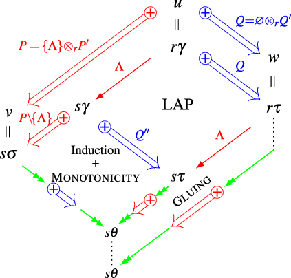
Figure 4. Non-overlapping case.
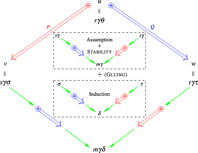
Figure 5. Overlapping case.
This terminates the proof of our main result. Note that we have not singled out either $\beta$
or small rules in the proof. The distinction is made without saying: the case
$\beta$
or small rules in the proof. The distinction is made without saying: the case $|O\cup O'|>1$
is impossible if
$|O\cup O'|>1$
is impossible if $i=\beta$
; and if
$i=\beta$
; and if $i\in{\mathcal{S}}$
, critical pairs only are possible if
$i\in{\mathcal{S}}$
, critical pairs only are possible if $j\in{\mathcal{S}}$
and parallel critical pairs if
$j\in{\mathcal{S}}$
and parallel critical pairs if $j\in{\mathcal{R}}$
; if
$j\in{\mathcal{R}}$
; if $i\in{\mathcal{R}}$
and
$i\in{\mathcal{R}}$
and $j\in{\mathcal{S}}$
, 1-nested critical pairs are also possible.
$j\in{\mathcal{S}}$
, 1-nested critical pairs are also possible.
5. Conclusion
Van Oostrom’s decreasing diagrams technique characterizes confluence of rewriting on an abstract set. It is well-known that its application to term rewriting is difficult, although many techniques were elaborated during the last years that successfully solved many open problems (Felgenhauer Reference Felgenhauer2013; Felgenhauer et al. Reference Felgenhauer, Middeldorp, Zankl and van Oostrom2015; Felgenhauer and van Oostrom Reference Felgenhauer and van Oostrom2013; Jouannaud and Liu Reference Jouannaud and Liu2012; Liu and Jouannaud Reference Liu and Jouannaud2014; Liu et al. Reference Liu, Jouannaud and Ogawa2015; Zankl et al. Reference Zankl, Felgenhauer and Middeldorp2015). For example, Felgenhauer proved that the existence of decreasing diagrams for parallel critical pairs ensures the confluence of non-terminating left-linear first-order rewriting systems (Felgenhauer and van Oostrom Reference Felgenhauer and van Oostrom2013).
Our main result, Theorem 4.2, shows that van Oostrom’s method applies to a quite complex new situation, higher-order rewriting of untyped terms with left-linear rules having non-trivial higher-order critical pairs. Compared to Felgenhauer’s, there are two new difficulties: rewrites are higher-order, and the presence of untyped $\beta$
-reductions. Compared to (Ferey and Jouannaud Reference Ferey and Jouannaud2019), we do not need the assumption that the set of higher-order rewrite rules defines a terminating relation, but can use the termination property of any subset of the rules, which has been proved very useful in examples. It is actually worth noting that if
$\beta$
-reductions. Compared to (Ferey and Jouannaud Reference Ferey and Jouannaud2019), we do not need the assumption that the set of higher-order rewrite rules defines a terminating relation, but can use the termination property of any subset of the rules, which has been proved very useful in examples. It is actually worth noting that if ${\mathcal{S}}={\mathcal{R}}$
, then nested critical pairs disappear as well as one-nested critical pairs. The result then reduces to the main theorem of (Ferey and Jouannaud Reference Ferey and Jouannaud2019), which appears to be subsumed by our new result. We have therefore got a new, powerful and flexible tool to prove the confluence on untyped terms of
${\mathcal{S}}={\mathcal{R}}$
, then nested critical pairs disappear as well as one-nested critical pairs. The result then reduces to the main theorem of (Ferey and Jouannaud Reference Ferey and Jouannaud2019), which appears to be subsumed by our new result. We have therefore got a new, powerful and flexible tool to prove the confluence on untyped terms of $\lambda$
-calculi augmented by left-linear higher-order rewrite rules.
$\lambda$
-calculi augmented by left-linear higher-order rewrite rules.
A main technical tool used here is the theory of orthogonal rewriting, which appears as being intimately related to van Oostrom’s multi-step rewriting (Terese 2003). One difference is that an orthogonal step uses different instances of a single rule at all orthogonal rewriting positions, whereas a multi-step may use instances of different rules. A main novel aspect of our definition is the associated notion of a nested critical pair and the corresponding critical pair property which allows us to check confluence of non-terminating higher-order definitions whose critical pairs are not development closed, as they are in (van Oostrom Reference van Oostrom1997). Nested critical pairs could of course be defined for multi-step rewriting by adapting our definitions, but this would result in an exponential blow up of their number, a strong argument in favor of orthogonal rewriting.
Higher-order rewriting definitions have been studied extensively in the past years because they allow us encoding program constructs in type theories such as Agda, <sc>Dedukti</sc> and Coq, which now all allow us for user-defined higher-order rules. They are also used in tools that target checking their confluence (Hamana Reference Hamana2017), or their termination (Kop Reference Kop2020). The examples we have carried out here, Plotkin–Power’s theory of global states and an encoding of lambda calculus used in <sc>Dedukti</sc>, illustrate the strength of orthogonal rewriting, which requires using nested critical pairs, as well as the use of small terminating rules, which only require plain critical pairs. Many other encoding examples appear in (Férey Reference Férey2021).
Our definition of higher-order rewriting for untyped $\lambda$
-terms is taken from (Ferey and Jouannaud Reference Ferey and Jouannaud2019). As is usual, rules have patterns for their left-hand sides, and pattern-matching and unification are higher-order, that is, in the context of patterns, modulo
$\lambda$
-terms is taken from (Ferey and Jouannaud Reference Ferey and Jouannaud2019). As is usual, rules have patterns for their left-hand sides, and pattern-matching and unification are higher-order, that is, in the context of patterns, modulo $\beta{^0}$
. What is crucial in this setting is the use of Klop’s notion of substitution for meta-variables with arities, which makes higher-order rewriting actually look like being first-order. The practical impact of this trick on technical developments is very impressive.
$\beta{^0}$
. What is crucial in this setting is the use of Klop’s notion of substitution for meta-variables with arities, which makes higher-order rewriting actually look like being first-order. The practical impact of this trick on technical developments is very impressive.
One may wonder whether it would be important to develop an abstract theory of orthogonal rewriting. This is indeed questionable. Orthogonal rewriting is needed in the presence of $\beta$
-reduction and of higher-order rules for three concurrent reasons that do not occur together otherwise: first,
$\beta$
-reduction and of higher-order rules for three concurrent reasons that do not occur together otherwise: first, $\beta$
-reduction does not terminate on untyped terms; second, higher-order rules generate
$\beta$
-reduction does not terminate on untyped terms; second, higher-order rules generate $\beta$
-redexes, which requires having maximal labels for the higher-order steps; third,
$\beta$
-redexes, which requires having maximal labels for the higher-order steps; third, $\beta$
-rewrites duplicate and stack their subexpressions, which requires using orthogonal higher-order rewriting steps in order to pack together many steps into one in order to meet the decreasing diagram condition for local peaks made of a
$\beta$
-rewrites duplicate and stack their subexpressions, which requires using orthogonal higher-order rewriting steps in order to pack together many steps into one in order to meet the decreasing diagram condition for local peaks made of a $\beta$
-redex sitting above a higher-order redex. The only other cases we can think of where these circumstances would be met are obtained by relaxing the constraints on the rewrite system added to untyped
$\beta$
-redex sitting above a higher-order redex. The only other cases we can think of where these circumstances would be met are obtained by relaxing the constraints on the rewrite system added to untyped $\beta$
-reduction, for example, by allowing us for non-left-linear rules.
$\beta$
-reduction, for example, by allowing us for non-left-linear rules.


 Open access