


1. Introduction
Category theory (by which we mean 1-category theory) is established as a convenient language to structure and discuss mathematical objects and morphisms between them. To axiomatize the fundamental objects of category theory itself – categories, functors, and natural transformations – the theory of 1-categories is not enough. Instead, category-like structures allowing for “morphisms between morphisms” were developed to account for the natural transformations. Among those structures are bicategories. Bicategory theory was originally developed by BÉnabou (Reference BÉnabou1967) in set-theoretic foundations. The goal of our work is to develop bicategory theory in univalent foundations. Specifically, we give a notion of a univalent bicategory and show that some bicategories of interest are univalent, with examples from algebra and type theory. To this end, we generalize (univalent) displayed categories of Ahrens and Lumsdaine (Reference Ahrens and Lumsdaine2019) to the bicategorical setting and prove that the total bicategory generated by a displayed bicategory is univalent, if the constituent pieces are. In addition, we show how to embed any bicategory with univalent hom-categories into a univalent bicategory via the Yoneda lemma, and we show how to use displayed machinery to construct biequivalences between total bicategories.
Univalent foundations and categories therein.
According to Voevodsky (Reference Voevodsky2014), a foundation of mathematics specifies, in particular, three things:
-
(1) a language for mathematical objects;
-
(2) a notion of proposition and proof; and
-
(3) an interpretation of those into a world of mathematical objects.
By “univalent foundations,” we mean the foundation given by univalent type theory as described, for example, in the HoTT book (Univalent Foundations Program 2013), with its notion of “univalent logic,” and the interpretation of univalent type theory in Kan complexes expected to arise from Voevodsky’s simplicial set model (Kapulkin and Lumsdaine Reference Kapulkin and Lumsdaine2021).
In the simplicial set model, univalent categories (just called “categories” by Ahrens et al. Reference Ahrens, Kapulkin and Shulman2015) correspond to truncated complete Segal spaces, which in turn are equivalent to ordinary (set-theoretic) categories. In this respect, univalent categories are “the right” notion of categories in univalent foundations: they correspond exactly to the traditional set-theoretic notion of category. Similarly, the notion of univalent bicategory, studied in this paper, provides the correct notion of bicategory in univalent foundations (Ahrens et al. Reference Ahrens, North, Shulman and Tsementzis2021, Example 9.1). In this work, we provide results for showing, modularly, that certain bicategories are univalent.
Throughout this article, we work in type theory with function extensionality. We explicitly mention any use of the univalence axiom. We use the notation standardized in the HoTT book (Univalent Foundations Program 2013); a significantly shorter overview of the setting we work in is given by Ahrens et al. (Reference Ahrens, Kapulkin and Shulman2015). As a reference for 1-category theory in univalent foundations, we refer to Ahrens et al. (Reference Ahrens, Kapulkin and Shulman2015), which follows a path suggested by Hofmann and Streicher (Reference Hofmann and Streicher1998), Section 5.5.
Motivation: bicategories for type theory.
One of the motivations for this work stems from several particular (classes of) bicategories that come up in our work on the semantics of type theories and Higher Inductive Types (HITs).
Firstly, we are interested in the “categories with structure” that have been used in the model theory of type theories. The purpose of the various categorical structures is to model context extension and substitution. Prominent such notions are categories with families (see, e.g., the work by Clairambault and Dybjer Reference Clairambault and Dybjer2014; Dybjer Reference Dybjer1995), categories with attributes (see, e.g., work by Pitts Reference Pitts2000), and categories with display maps (see, e.g., work by North Reference North2019; Taylor Reference Taylor1999). Each notion of “categorical structure” gives rise to a bicategory whose objects are categories equipped with such a structure. In the present work, we provide machinery that can be used to show, in a modular way, that these bicategories are univalent; we exemplify the machinery with categories with families.
Secondly, Dybjer and Moeneclaey (Reference Dybjer and Moeneclaey2018) define a notion of signature for 1-HITs and study algebras of those signatures. These algebras are groupoids equipped with extra structure according to the signature. In the present work, we give general methods for constructing bicategories of such algebras and we demonstrate the usage of those methods by constructing the bicategory of monads internal to a given bicategory. We then construct a bicategory of Kleisli triples (an alternative presentation of monads Footnote 1 ) and show that it is equivalent to the bicategory of monads. We also show that the resulting bicategory of monads internal to the bicategory of univalent categories is biequivalent to the bicategory of Kleisli triples.
Technical contribution: displayed bicategories.
In this work, we develop the notion of displayed bicategory in analogy to the 1-categorical notion of displayed category introduced by Ahrens and Lumsdaine (Reference Ahrens and Lumsdaine2019). Intuitively, a displayed bicategory $\mathsf{D}$
over a bicategory
$\mathsf{D}$
over a bicategory $\mathsf{B}$
represents data and properties to be added to
$\mathsf{B}$
represents data and properties to be added to $\mathsf{B}$
to form a new bicategory:
$\mathsf{B}$
to form a new bicategory: $\mathsf{D}$
gives rise to the total bicategory
$\mathsf{D}$
gives rise to the total bicategory ${\textstyle \int_{\mathsf{D}}{}}$
. Its cells are pairs (b,d) where d in
${\textstyle \int_{\mathsf{D}}{}}$
. Its cells are pairs (b,d) where d in $\mathsf{D}$
is a “displayed cell” over b in
$\mathsf{D}$
is a “displayed cell” over b in $\mathsf{B}$
. Univalence of
$\mathsf{B}$
. Univalence of ${\textstyle \int_{\mathsf{D}}{}}$
can be shown from univalence of
${\textstyle \int_{\mathsf{D}}{}}$
can be shown from univalence of $\mathsf{B}$
and “displayed univalence” of
$\mathsf{B}$
and “displayed univalence” of $\mathsf{D}$
. The latter two conditions are easier to show, sometimes significantly easier.
$\mathsf{D}$
. The latter two conditions are easier to show, sometimes significantly easier.
Two features make the displayed point of view particularly useful: firstly, displayed structures can be iterated, making it possible to build bicategories of very complicated objects layerwise. Secondly, displayed “building blocks” can be provided, for which univalence is proved once and for all. These building blocks, for example, the Cartesian product, can be used like LEGO ${}^{\small\textrm{TM}}$
pieces to modularly build bicategories of large structures that are automatically accompanied by a proof of univalence.
${}^{\small\textrm{TM}}$
pieces to modularly build bicategories of large structures that are automatically accompanied by a proof of univalence.
We demonstrate these features in examples, proving univalence of three important (classes of) bicategories: first, the bicategory of pseudofunctors between two univalent bicategories; second, bicategories of algebraic structures (given as pseudoalgebras of pseudofunctors); and third, the bicategory of categories with families.
Main contributions.
Here we give a list of the main results presented in this paper:
Following the construction of the Rezk completion for categories by Ahrens et al. (Reference Ahrens, Kapulkin and Shulman2015), Theorem 8.5, we show in sec:yoneda that every locally univalent bicategory embeds into a univalent one. This result fundamentally relies on the proof of a bicategorical version of the Yoneda lemma.
We develop displayed infrastructure for bicategories and show that it is useful for building bicategories. In particular, we modularly prove univalence of complicated bicategories in sec:examples, such as the bicategory of pseudofunctors between two univalent bicategories, the bicategory of pseudoalgebras of a given pseudofunctor, and the bicategory of categories with families.
We show the benefits of the displayed infrastructure for defining morphisms between bicategories in layers. We demonstrate this on two examples in sec:dispconstr: the construction of a biequivalence between pointed 1-types and pointed univalent groupoids and the construction of a biequivalence between monads internal to the bicategory of univalent categories and the bicategory of Kleisli triples.
Formalization.
The results presented here are mechanized in the UniMath library (Voevodsky et al. Reference Voevodsky, Ahrens and Grayson2021), which is based on the Coq proof assistant (Coq Development Team 2019). The UniMath library is under constant development; in this paper, we refer to the version with git hash c26d11b. Throughout the paper, definitions and statements are accompanied by a link to the online documentation of that version. For instance, the link bicat points to the definition of a bicategory.
Related work.
Our work extends the notion of univalence from 1-categories (Ahrens et al. Reference Ahrens, Kapulkin and Shulman2015) to bicategories. Similarly, we extend the notion of displayed 1-category (Ahrens and Lumsdaine Reference Ahrens and Lumsdaine2019) to the bicategorical setting.
Ahrens et al. (Reference Ahrens, North, Shulman and Tsementzis2020) devise a notion of “signature” and “theory” for mathematical structures. To each theory they associate a type of models of that theory and a predicate of “being univalent” on such models. Their signatures encompass, in particular, bicategories (Ahrens et al. Reference Ahrens, North, Shulman and Tsementzis2021, Example 9.1), more specifically, saturated ana-bicategories. Ana-bicategories that are both saturated and univalent should correspond to the univalent bicategories studied here, even though a formal statement and construction of a suitable equivalence is outside the scope of the present work.
Capriotti and Kraus (Reference Capriotti and Kraus2018) study univalent (n,1)-categories for $n \in \{0,1,2\}$
. They only consider bicategories where the 2-cells are equalities between 1-cells; in particular, all 2-cells considered there are invertible, and their (2,1)-categories are by definition locally univalent (cf. Definition 3.1, Item 1). Consequently, the condition called univalence by Capriotti and Kraus is what we call global univalence, cf. Definition 3.1, Item 2. In this work, we study bicategories, a.k.a. (weak) (2,2)-categories, that is, we allow for non-invertible 2-cells. The examples we study in sec:examples are proper (2,2)-categories and are not covered by Capriotti and Kraus (Reference Capriotti and Kraus2018).
$n \in \{0,1,2\}$
. They only consider bicategories where the 2-cells are equalities between 1-cells; in particular, all 2-cells considered there are invertible, and their (2,1)-categories are by definition locally univalent (cf. Definition 3.1, Item 1). Consequently, the condition called univalence by Capriotti and Kraus is what we call global univalence, cf. Definition 3.1, Item 2. In this work, we study bicategories, a.k.a. (weak) (2,2)-categories, that is, we allow for non-invertible 2-cells. The examples we study in sec:examples are proper (2,2)-categories and are not covered by Capriotti and Kraus (Reference Capriotti and Kraus2018).
Outside of univalent foundations, there are also computer-checked libraries of bicategory theory, see, for example, work by Stark (Reference Stark2020), Hu and Carette (Reference Hu and Carette2021).
Publication history.
This article is an extended version of a conference contribution (Ahrens et al. Reference Ahrens, Frumin, Maggesi and van der Weide2019). Compared to the conference version, we have added the following content:
In Section 2, we define the notion of biequivalence of bicategories, the “correct” notion of sameness for bicategories. We construct a biequivalence between 1-types and univalent groupoids.
In Section 3, we present an induction principle for invertible 2-cells in a locally univalent bicategory and an induction principle for adjoint equivalences in a globally univalent bicategory. We put these principles to work in a number of examples.
Section 4 is new. In there, we propose a definition of 2-category and of strict bicategory, and we show that these are equivalent.
Section 5 is new. In there, we show that any bicategory embeds into a univalent one via the Yoneda embedding. This construction is reminiscent of the Rezk completion for categories.
In Section 6, we give the definition of the displayed bicategory of monads internal to a given bicategory and the displayed bicategory of Kleisli triples. The bicategory of monads on a bicategory $\mathsf{B}$
is univalent whenever
$\mathsf{B}$
is univalent, which is proved in Section 9.2.
$\mathsf{B}$
is univalent whenever
$\mathsf{B}$
is univalent, which is proved in Section 9.2.Section 8 is new. In there, we introduce the notion of displayed biequivalence. Using this notion, we show that the biequivalence between 1-types and univalent groupoids extends to a biequivalence between their pointed variants. We also construct a biequivalence between the bicategory of Kleisli triples and the bicategory of monads internal to the bicategory of univalent categories.
Section 10 is new. Following a suggestion by an anonymous referee, we generalize the constructions in Sections 9.2 and 9.3 using displayed inserters.


2. Bicategories and Some Examples
Bicategories were introduced by BÉnabou (Reference BÉnabou1967), encompassing monoidal categories, 2-categories (in particular, the 2-category of categories), and other examples. He (and later many other authors) defines bicategories in the style of “categories weakly enriched in categories.” That is, the hom-objects $\mathsf{B}_1(a,b)$
of a bicategory
$\mathsf{B}_1(a,b)$
of a bicategory $\mathsf{B}$
are taken to be (1-)categories, and composition is given by a functor
$\mathsf{B}$
are taken to be (1-)categories, and composition is given by a functor $\mathsf{B}_1(a,b)\times \mathsf{B}_1(b,c) \to \mathsf{B}_1(a,c)$
. This presentation of bicategories is concise and convenient for communication between mathematicians.
$\mathsf{B}_1(a,b)\times \mathsf{B}_1(b,c) \to \mathsf{B}_1(a,c)$
. This presentation of bicategories is concise and convenient for communication between mathematicians.
In this article, we use a different, more unfolded definition of bicategories, which is inspired by BÉnabou (Reference BÉnabou1967), Section 1.3 and nLab authors (2018), Section “Details”. One the one hand, it is more verbose than the definition via weak enrichment. On the other hand, it is better suited for our purposes; in particular, it is suitable for defining displayed bicategories, cf. Section 6.
Definition 2.1 (prebicat, bicat). A prebicategory $\mathsf{B}$
consists of
$\mathsf{B}$
consists of
-
(1) a type
$\mathsf{B}_0$
of objects; -
(2) a type
$\mathsf{B}_1(a, b)$
of 1-cells for all
$a, b : \mathsf{B}_0$
; -
(3) a type
$\mathsf{B}_2(f, g)$
of 2-cells for all
$a, b : \mathsf{B}_0$
and
$f, g : \mathsf{B}_1(a,b)$
; -
(4) an identity 1-cell
$\operatorname{id}_1\!(a) : \mathsf{B}_1(a,a)$
; -
(5) a composition
$\mathsf{B}_1(a,b) \times \mathsf{B}_1(b,c) \rightarrow \mathsf{B}_1(a,c)$
, written
$f \cdot g$
; -
(6) an identity 2-cell
$\operatorname{id}_2\!(f) : \mathsf{B}_2(f,f)$
; -
(7) a vertical composition
$\theta \bullet \gamma : \mathsf{B}_2(f,h)$
for all 1-cells
$f,g,h : \mathsf{B}_1(a,b)$
and 2-cells
$\theta : \mathsf{B}_2(f,g)$
and
$\gamma : \mathsf{B}_2(g,h)$
; -
(8) a left whiskering
$f \vartriangleleft \theta : \mathsf{B}_2(f \cdot g, f \cdot h)$
for all 1-cells
$f : \mathsf{B}_1(a,b)$
and
$g,h : \mathsf{B}_1(b,c)$
and 2-cells
$\theta : \mathsf{B}_2(g,h)$
; -
(9) a right whiskering
$\theta \vartriangleright h : \mathsf{B}_2(f \cdot h, g \cdot h)$
for all 1-cells
$f, g : \mathsf{B}_1(a,b)$
and
$h : \mathsf{B}_1(b,c)$
and 2-cells
$\theta : \mathsf{B}_2(f,g)$
; -
(10) a left unitor
$\lambda(f) : \mathsf{B}_2({\operatorname{id}}_1(a) \cdot f,f)$
and its inverse
$\lambda(f)^{-1} : \mathsf{B}_2(f,\operatorname{id}_1\!(a) \cdot f)$
; -
(11) a right unitor
$\rho(f) : \mathsf{B}_2(f \cdot \operatorname{id}_1\!(b),f)$
and its inverse
$\rho(f)^{-1} : \mathsf{B}_2(f,f \cdot \operatorname{id}_1\!(b))$
; -
(12) a left associator
$\alpha(f,g,h) : \mathsf{B}_2(f \cdot (g \cdot h), (f \cdot g) \cdot h)$
and a right associator
$\alpha(f,g,h)^{-1} : \mathsf{B}_2((f \cdot g) \cdot h, f \cdot (g \cdot h))$
for
$f : \mathsf{B}_1(a,b)$
,
$g : \mathsf{B}_1(b,c)$
, and
$h : \mathsf{B}_1(c,d)$


such that, for all suitable objects, 1-cells, and 2-cells,
-
(13)
$\operatorname{id}_2\!(f) \bullet \theta = \theta, \quad \theta \bullet \operatorname{id}_2\!(g) = \theta, \quad \theta \bullet (\gamma \bullet \tau) = (\theta \bullet \gamma) \bullet \tau$
; -
(14)
$f \vartriangleleft ({\operatorname{id}}_2 g) = \operatorname{id}_2\!(f \cdot g), \quad f \vartriangleleft (\theta \bullet \gamma) = (f \vartriangleleft \theta) \bullet (f \vartriangleleft \gamma)$
; -
(15)
$({\operatorname{id}}_2 f) \vartriangleright g = \operatorname{id}_2\!(f \cdot g), \quad (\theta \bullet \gamma) \vartriangleright g = (\theta \vartriangleright g) \bullet (\gamma \vartriangleright g)$
; -
(16)
$({\operatorname{id}}_1(a) \vartriangleleft \theta) \bullet \lambda(g) = \lambda(f) \bullet \theta$
; -
(17)
$(\theta \vartriangleright \operatorname{id}_1\!(b)) \bullet \rho(g) = \rho(f) \bullet \theta$
; -
(18)
$(f \vartriangleleft (g \vartriangleleft \theta)) \bullet \alpha(f, g, i) = \alpha(f,g,h) \bullet ((f \cdot g) \vartriangleleft \theta)$
; -
(19)
$(f \vartriangleleft (\theta \vartriangleright i)) \bullet \alpha(f,h,i) = \alpha(f,g,i) \bullet ((f \vartriangleleft \theta) \vartriangleright i)$
; -
(20)
$(\theta \vartriangleright (h \cdot i)) \bullet \alpha(g,h,i) = \alpha(f,h,i) \bullet ((\theta \vartriangleright h) \vartriangleright i)$
; -
(21)
$(\theta \vartriangleright h) \bullet (g \vartriangleleft \gamma) = (f \vartriangleleft \gamma) \bullet (\theta \vartriangleright i)$
; -
(22)
$\lambda(f) \bullet \lambda(f)^{-1} = \operatorname{id}_2\!({\operatorname{id}}_1(a) \cdot f), \quad \lambda(f)^{-1} \bullet \lambda(f) = \operatorname{id}_2\!(f)$
; -
(23)
$\rho(f) \bullet \rho(f)^{-1} = \operatorname{id}_2\!(f \cdot \operatorname{id}_1\!(b)), \quad \rho(f)^{-1} \bullet \rho(f) = \operatorname{id}_2\!(f)$
; -
(24)
$\alpha(f,g,h) \bullet \alpha(f,g,h)^{-1} = \operatorname{id}_2\!(f \cdot (g \cdot h)), \quad \alpha(f,g,h)^{-1} \bullet \alpha(f,g,h) = \operatorname{id}_2\!((f \cdot g) \cdot h)$
; -
(25)
$\alpha(f, \operatorname{id}_1\!(b),g) \bullet (\rho(f) \vartriangleright g) = f \vartriangleleft \lambda(g)$
; -
(26)
$\alpha(f,g,h \cdot i) \bullet \alpha(f \cdot g, h, i) = (f \vartriangleleft \alpha(g,h,i)) \bullet \alpha(f,g \cdot h, i) \bullet (\alpha(f,g,h) \vartriangleright i)$
.


A bicategory is a prebicategory whose types of 2-cells $\mathsf{B}_2(f,g)$
are sets for all
$\mathsf{B}_2(f,g)$
are sets for all $a,b : \mathsf{B}_0$
and
$a,b : \mathsf{B}_0$
and $f,g : \mathsf{B}_1(a,b)$
.
$f,g : \mathsf{B}_1(a,b)$
.
We write $a \rightarrow b$
for
$a \rightarrow b$
for $\mathsf{B}_1(a,b)$
and
$\mathsf{B}_1(a,b)$
and $f \Rightarrow g$
for
$f \Rightarrow g$
for $\mathsf{B}_2(f,g)$
.
$\mathsf{B}_2(f,g)$
.
Mitchell Riley formalized a definition of bicategories as “categories weakly enriched in categories” in UniMath, based on work by Peter LeFanu Lumsdaine. We do not reproduce this definition here; it is available as prebicategory. That definition is equivalent to our definition, in the following sense:
Proposition 2.2 (weq-bicat-prebicategory) The type of bicategories defined in def:bicat is equivalent to the type of bicategories in terms of weak enrichment.
For this result, one needs to show that each $\mathsf{B}_1(a,b)$
forms a category whose morphisms are 2-cells. Let us introduce this formally.
$\mathsf{B}_1(a,b)$
forms a category whose morphisms are 2-cells. Let us introduce this formally.
Definition 2.3 (hom) Let $\mathsf{B}$
be a bicategory and
$\mathsf{B}$
be a bicategory and $a, b : \mathsf{B}_0$
objects of
$a, b : \mathsf{B}_0$
objects of $\mathsf{B}$
. Then, we define the hom-category
$\mathsf{B}$
. Then, we define the hom-category $\underline{{\mathsf{B}_1}({a},{b})}$
to be the category whose objects are 1-cells
$\underline{{\mathsf{B}_1}({a},{b})}$
to be the category whose objects are 1-cells $f : a \rightarrow b$
and whose morphisms from f to g are 2-cells
$f : a \rightarrow b$
and whose morphisms from f to g are 2-cells $\alpha : f \Rightarrow g$
of
$\alpha : f \Rightarrow g$
of $\mathsf{B}$
. The identity morphisms are identity 2-cells, and the composition is vertical composition of 2-cells.
$\mathsf{B}$
. The identity morphisms are identity 2-cells, and the composition is vertical composition of 2-cells.
Recall that our goal is to study univalence of bicategories, which is a property that relates equivalence and equality. For this reason, we study the two analogs of the 1-categorical notion of isomorphism. The corresponding notion for 2-cells is that of invertible 2-cells.
Definition 2.4 ((is_invertible_2cell)) A 2-cell $\theta : f \Rightarrow g$
is called invertible if we have
$\theta : f \Rightarrow g$
is called invertible if we have $\gamma : g \Rightarrow f$
such that
$\gamma : g \Rightarrow f$
such that $\theta \bullet \gamma = \operatorname{id}_2\!(f)$
and
$\theta \bullet \gamma = \operatorname{id}_2\!(f)$
and $\gamma \bullet \theta = \operatorname{id}_2\!(g)$
. An invertible 2-cell consists of a 2-cell and a proof that it is invertible, and
$\gamma \bullet \theta = \operatorname{id}_2\!(g)$
. An invertible 2-cell consists of a 2-cell and a proof that it is invertible, and $\mathsf{inv2cell}(f,g)$
is the type of invertible 2-cells from f to g.
$\mathsf{inv2cell}(f,g)$
is the type of invertible 2-cells from f to g.
Since 2-cells form a set and inverses are unique, being an invertible 2-cell is a proposition. In addition, $\operatorname{id}_2\!(f)$
is invertible, and we write
$\operatorname{id}_2\!(f)$
is invertible, and we write $\operatorname{id}_2\!(f) : \mathsf{inv2cell}(f,f)$
for this invertible 2-cell.
$\operatorname{id}_2\!(f) : \mathsf{inv2cell}(f,f)$
for this invertible 2-cell.
The bicategorical analog of isomorphisms for 1-cells is the notion of adjoint equivalence.
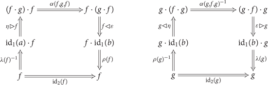
Definition 2.5 ((adjoint_equivalence)) An adjoint equivalence structure on a 1-cell $f: a \rightarrow b$
consists of a 1-cell
$f: a \rightarrow b$
consists of a 1-cell $g : b \rightarrow a$
and invertible 2-cells
$g : b \rightarrow a$
and invertible 2-cells $\eta : \operatorname{id}_1\!(a) \Rightarrow f \cdot g$
and
$\eta : \operatorname{id}_1\!(a) \Rightarrow f \cdot g$
and $\varepsilon : g \cdot f \Rightarrow \operatorname{id}_1\!(b)$
such that the following two diagrams commute
$\varepsilon : g \cdot f \Rightarrow \operatorname{id}_1\!(b)$
such that the following two diagrams commute
An adjoint equivalence consists of a 1-cell f together with an adjoint equivalence structure on f. The type $\mathsf{AdjEquiv}({a},{b})$
consists of all adjoint equivalences from a to b.
$\mathsf{AdjEquiv}({a},{b})$
consists of all adjoint equivalences from a to b.
We call $\eta$
and
$\eta$
and $\varepsilon$
the unit and counit of the adjoint equivalence, and we call g the right adjoint. The prime example of an adjoint equivalence is the identity 1-cell
$\varepsilon$
the unit and counit of the adjoint equivalence, and we call g the right adjoint. The prime example of an adjoint equivalence is the identity 1-cell $\operatorname{id}_1\!(a),$
and we denote it by
$\operatorname{id}_1\!(a),$
and we denote it by $\operatorname{id}_1\!(a) : \mathsf{AdjEquiv}({a},{a})$
. Sometimes, we write
$\operatorname{id}_1\!(a) : \mathsf{AdjEquiv}({a},{a})$
. Sometimes, we write $a \simeq b$
for
$a \simeq b$
for $\mathsf{AdjEquiv}({a},{b})$
.
$\mathsf{AdjEquiv}({a},{b})$
.
Before we start our study of univalence, we present some examples of bicategories and preliminary notions from bicategory theory.
Example 2.6 (fundamental_bigroupoid).Let X be a 2-type. Then, we define the fundamental bigroupoid $\pi({X})$
to be the bicategory whose 0-cells are inhabitants of X, 1-cells from x to y are paths
$\pi({X})$
to be the bicategory whose 0-cells are inhabitants of X, 1-cells from x to y are paths $x = y$
, and 2-cells from p to q are higher-order paths
$x = y$
, and 2-cells from p to q are higher-order paths $p = q$
. The operations, such as composition and whiskering, are defined using path induction. Every 1-cell is an adjoint equivalence and every 2-cell is invertible.
$p = q$
. The operations, such as composition and whiskering, are defined using path induction. Every 1-cell is an adjoint equivalence and every 2-cell is invertible.
Example 2.7 ((one_types)) Let $\operatorname{\textsf{U}}$
be a universe. The objects of the bicategory
$\operatorname{\textsf{U}}$
be a universe. The objects of the bicategory $\mbox{1-}\mathsf{Type}_{\operatorname{\textsf{U}}}$
are 1-truncated types of the universe
$\mbox{1-}\mathsf{Type}_{\operatorname{\textsf{U}}}$
are 1-truncated types of the universe $\operatorname{\textsf{U}}$
, the 1-cells are functions between the underlying types, and the 2-cells are homotopies between functions. The 1-cells
$\operatorname{\textsf{U}}$
, the 1-cells are functions between the underlying types, and the 2-cells are homotopies between functions. The 1-cells $\operatorname{id}_1\!(X)$
and
$\operatorname{id}_1\!(X)$
and $f \cdot g$
are defined as the identity and composition of functions, respectively. The 2-cell
$f \cdot g$
are defined as the identity and composition of functions, respectively. The 2-cell $\operatorname{id}_2\!(f)$
is
$\operatorname{id}_2\!(f)$
is $\operatorname{\mathsf{{refl}}}$
, the 2-cell
$\operatorname{\mathsf{{refl}}}$
, the 2-cell $p \bullet q$
is the concatenation of paths. The unitors and associators are defined as identity paths. Every 2-cell is invertible, and adjoint equivalences from X to Y are the same as equivalences of types from X to Y.
$p \bullet q$
is the concatenation of paths. The unitors and associators are defined as identity paths. Every 2-cell is invertible, and adjoint equivalences from X to Y are the same as equivalences of types from X to Y.
Example 2.8 ((bicat_of_univ_cats)) We define the bicategory $\mathsf{Cat}$
of univalent categories as the bicategory whose 0-cells are univalent categories, 1-cells are functors, and 2-cells are natural transformations. The identity 1-cells are identity functors, the composition and whiskering operations are composition of functors and whiskering of functors and transformations, respectively. Invertible 2-cells are natural isomorphisms, and adjoint equivalences are external adjoint equivalences of categories.
$\mathsf{Cat}$
of univalent categories as the bicategory whose 0-cells are univalent categories, 1-cells are functors, and 2-cells are natural transformations. The identity 1-cells are identity functors, the composition and whiskering operations are composition of functors and whiskering of functors and transformations, respectively. Invertible 2-cells are natural isomorphisms, and adjoint equivalences are external adjoint equivalences of categories.
Example 2.9 ((op1_bicat)) Let $\mathsf{B}$
be a bicategory. Then we define
$\mathsf{B}$
be a bicategory. Then we define $\mathsf{B}^{\operatorname{\mathsf{{op}}}}$
to be the bicategory whose objects are objects in
$\mathsf{B}^{\operatorname{\mathsf{{op}}}}$
to be the bicategory whose objects are objects in $\mathsf{B}$
, 1-cells from x to y are 1-cells
$\mathsf{B}$
, 1-cells from x to y are 1-cells $y \rightarrow x$
in
$y \rightarrow x$
in $\mathsf{B}$
, and the 2-cells from f to g are 2-cells
$\mathsf{B}$
, and the 2-cells from f to g are 2-cells $f \Rightarrow g$
in
$f \Rightarrow g$
in $\mathsf{B}$
.
$\mathsf{B}$
.
Definition 2.10 ((fullsubbicat)) Let $\mathsf{B}$
be a bicategory and
$\mathsf{B}$
be a bicategory and $P : \mathsf{B}_0 \to \operatorname{\textsf{hProp}}$
a predicate on the 0-cells of
$P : \mathsf{B}_0 \to \operatorname{\textsf{hProp}}$
a predicate on the 0-cells of $\mathsf{B}$
. We define the full subbicategory of
$\mathsf{B}$
. We define the full subbicategory of $\mathsf{B}$
with 0-cells satisfying P as the bicategory whose objects are pairs
$\mathsf{B}$
with 0-cells satisfying P as the bicategory whose objects are pairs $(a,p_a) : \sum_{(x : \mathsf{B}_0)} . P (x)$
, 1-cells from
$(a,p_a) : \sum_{(x : \mathsf{B}_0)} . P (x)$
, 1-cells from $(a,p_a)$
to
$(a,p_a)$
to $(b,p_b)$
are 1-cells
$(b,p_b)$
are 1-cells $a \rightarrow b$
in
$a \rightarrow b$
in $\mathsf{B}$
, and 2-cells are as in
$\mathsf{B}$
, and 2-cells are as in $\mathsf{B}$
. In Example 6.5, we present a construction of this bicategory using displayed bicategories.
$\mathsf{B}$
. In Example 6.5, we present a construction of this bicategory using displayed bicategories.
Example 2.11 ((grpds)) We define the bicategory $\mathsf{Grpd}$
as the full subbicategory of
$\mathsf{Grpd}$
as the full subbicategory of $\mathsf{Cat}$
in which every object is a groupoid.
$\mathsf{Cat}$
in which every object is a groupoid.
For 1-categories, the “correct” notion of equality is not isomorphism of categories, but equivalence of categories. Similarly, the right notion of equality for bicategories is biequivalence. To talk about biequivalences, we need to introduce pseudofunctors.
Definition 2.12 ((psfunctor)) Let $\mathsf{B}$
and
$\mathsf{B}$
and $\mathsf{C}$
be bicategories. A pseudofunctor F from
$\mathsf{C}$
be bicategories. A pseudofunctor F from $\mathsf{B}$
to
$\mathsf{B}$
to $\mathsf{C}$
consists of
$\mathsf{C}$
consists of
A function
$F_0 : \mathsf{B}_0 \rightarrow \mathsf{C}_0$
;For all
$a, b : \mathsf{B}_0$
, a function
$F_1 : \mathsf{B}_1(a, b) \rightarrow \mathsf{C}_1(F_0(a), F_0(b))$
;For all
$f, g : \mathsf{B}_1(a, b)$
, a function
$F_2 : \mathsf{B}_2(f, g) \rightarrow \mathsf{C}_2(F_1(f), F_1(g))$
;For each
$a : \mathsf{B}_0$
an invertible 2-cell
${{F}(a)}_i : \operatorname{id}_1\!(F_0(a)) \Rightarrow F_1({\operatorname{id}}_1(a))$
;For each
$f : \mathsf{B}_1(a, b)$
and
$g : \mathsf{B}_1(b, c)$
, an invertible 2-cell
${F}_c(f, g) : F_1(f) \cdot F_1(g) \Rightarrow F_1(f \cdot g)$


such that
 \begin{equation*}F_2({\operatorname{id}}_2(f)) = \operatorname{id}_2\!(F_1(f)) \quad \quad F_2(f \bullet g) = F_2(f) \bullet F_2(g)\end{equation*}
and such that the following diagrams commute (where all free variables should be taken to be universally quantified):


We write ${\mathsf{B}} \rightarrow {\mathsf{C}}$
for the type of pseudofunctors from
${\mathsf{B}} \rightarrow {\mathsf{C}}$
for the type of pseudofunctors from $\mathsf{B}$
to
$\mathsf{B}$
to $\mathsf{C}$
.
$\mathsf{C}$
.
In the remainder of the paper, we sometimes write F(a) instead of $F_0(a)$
, and we use the same convention for
$F_0(a)$
, and we use the same convention for $F_1$
and
$F_1$
and $F_2$
. We call the 2-cells
$F_2$
. We call the 2-cells ${{F}}_i$
and
${{F}}_i$
and ${F}_c$
the identitor and compositor, respectively. From each pseudofunctor
${F}_c$
the identitor and compositor, respectively. From each pseudofunctor $F : \mathsf{B} \rightarrow \mathsf{C}$
we can assemble functors
$F : \mathsf{B} \rightarrow \mathsf{C}$
we can assemble functors $F_1(a, b) : \underline{{\mathsf{B}_1}({a},{b})} \rightarrow \underline{{\mathsf{C}_1}({F(a)},{F(b)})}$
between the hom-categories.
$F_1(a, b) : \underline{{\mathsf{B}_1}({a},{b})} \rightarrow \underline{{\mathsf{C}_1}({F(a)},{F(b)})}$
between the hom-categories.
Definition 2.13 ((pstrans)) Let $\mathsf{B}$
and
$\mathsf{B}$
and $\mathsf{C}$
be bicategories and
$\mathsf{C}$
be bicategories and $F, G : \mathsf{B} \rightarrow \mathsf{C}$
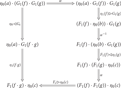
pseudofunctors between them. Then, a pseudotransfomation
$F, G : \mathsf{B} \rightarrow \mathsf{C}$
pseudofunctors between them. Then, a pseudotransfomation $\eta$
from F to G consists of
$\eta$
from F to G consists of
For each
$a : \mathsf{B}_0$
a 1-cell
$\eta_0(a) : F_0(a) \rightarrow G_0(a)$
;For each
$a, b : \mathsf{B}_0$
and
$f : \mathsf{B}_1(a, b)$
, an invertible 2-cell
$\eta_1(f) : \eta_0 (a) \cdot G_1(f) \Rightarrow F_1(g) \cdot \eta_0(b)$


such that the following diagrams commute

We write ${F} \Rightarrow {G}$
for the type of pseudotransformations from F to G.
${F} \Rightarrow {G}$
for the type of pseudotransformations from F to G.
Definition 2.14 ((modification)) Let $\mathsf{B}$
and
$\mathsf{B}$
and $\mathsf{C}$
be bicategories,
$\mathsf{C}$
be bicategories, $F, G : \mathsf{B} \rightarrow \mathsf{C}$
be pseudofunctors, and
$F, G : \mathsf{B} \rightarrow \mathsf{C}$
be pseudofunctors, and $\eta, \theta : {F} \Rightarrow {G}$
be pseudotransformations. A modification
$\eta, \theta : {F} \Rightarrow {G}$
be pseudotransformations. A modification $\Gamma$
from
$\Gamma$
from $\eta$
to
$\eta$
to $\theta$
consists of 2-cells
$\theta$
consists of 2-cells $\Gamma(a) : \eta(a) \Rightarrow \theta(a)$
for each
$\Gamma(a) : \eta(a) \Rightarrow \theta(a)$
for each $a : \mathsf{B}$
such that
$a : \mathsf{B}$
such that
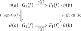
commutes for any $a, b : \mathsf{B}$
and
$a, b : \mathsf{B}$
and $f : \mathsf{B}_1(a, b)$
. We write
$f : \mathsf{B}_1(a, b)$
. We write ${\eta} \Rrightarrow {\theta}$
for the type of modifications from
${\eta} \Rrightarrow {\theta}$
for the type of modifications from $\eta$
to
$\eta$
to $\theta$
.
$\theta$
.
To illustrate these three definitions, we look at some examples.
Example 2.15. Let X and Y be 2-types.
(ap_psfunctor) Each function
$f : X \rightarrow Y$
induces a pseudofunctor
$\overline{f} : {\pi({X})} \rightarrow {\pi({Y})}$
, which sends objects
$x : X$
to f(x), 1-cells
$p : x = y$
to
$\mathsf{ap} \ {f} \ {p}$
, and 2-cells
$h : p = q$
to
$\mathsf{ap} \ {(\mathsf{ap} \ f)} \ {h}$
.(ap_pstrans) Suppose we have
$f, g : X \rightarrow Y$
and
$e : \prod_{x : X} f(x) = g(x)$
. Then we obtain a pseudotransformation
$\overline{e} : {\overline{f}} \Rightarrow {\overline{g}}$
whose component at x is e(x), and whose actions on 1-cells are given by path induction.(ap_modification) Let
$f, g : X \rightarrow Y$
and
$e_1, e_2 : \prod_{x : X} f(x) = g(x)$
. Then each family of paths
$h : \prod_{x : X} e_1(x) = e_2(x)$
gives rise to a modification
$\overline{h} : {\overline{e_1}} \Rrightarrow {\overline{e_2}}$
whose component at x is h(x).


Example 2.16 We have the following pseudofunctors and pseudotransformations:
(id_psfunctor) Given a bicategory
$\mathsf{B}$
, we have the identity pseudofunctor
$\operatorname{id}(\mathsf{B})$
from
$\mathsf{B}$
to
$\mathsf{B}$
. Its action on 0-cells, 1-cells, and 2-cells is the identity.(comp_psfunctor) Given bicategories
$\mathsf{B}_1$
,
$\mathsf{B}_2$
, and
$\mathsf{B}_3$
and pseudofunctors
$F : {\mathsf{B}_1} \rightarrow {\mathsf{B}_2}$
and
$G : {\mathsf{B}_2} \rightarrow {\mathsf{B}_3}$
, then we have a pseudofunctor
$F \cdot G$
from
$\mathsf{B}_1$
to
$\mathsf{B}_3$
. It sends objects a to
$G_0(F_0(a))$
, 1-cells f to
$G_1(F_1(f))$
, and 2-cells
$\theta$
to
$G_2(F_2(\theta))$
.(id_pstrans) Given bicategories
$\mathsf{B}_1$
and
$\mathsf{B}_2$
and a pseudofunctor
$F : {\mathsf{B}_1} \rightarrow {\mathsf{B}_2}$
, we have a pseudotransformation
$\operatorname{id}(F)$
from F to F. It sends objects a to
$\operatorname{id}_1\!(F_1(a))$
, and similarly for 1-cells.(comp_pstrans) Given bicategories
$\mathsf{B}_1$
and
$\mathsf{B}_2$
, pseudofunctors
$F, G, H : {\mathsf{B}_1} \rightarrow {\mathsf{B}_2}$
, and two pseudotransformations
$\theta_1 : {F} \Rightarrow {G}$
and
$\theta_2 : {G} \Rightarrow {H}$
, we have a pseudotransformation
$\eta_1 \bullet \eta_2 : {F} \Rightarrow {H}$
. It sends objects a to
$\theta_1(a) \cdot \theta_2(a)$
.


Note that we have a bicategory $\mathsf{Pseudo}(\mathsf{B}, \mathsf{C})$
of pseudofunctors, pseudotransformations, and modifications. We construct this bicategory in section 9.1 using displayed bicategories, and then, we define invertible modifications to be invertible 2-cells in this bicategory. With all this in place, we can define biequivalences.
$\mathsf{Pseudo}(\mathsf{B}, \mathsf{C})$
of pseudofunctors, pseudotransformations, and modifications. We construct this bicategory in section 9.1 using displayed bicategories, and then, we define invertible modifications to be invertible 2-cells in this bicategory. With all this in place, we can define biequivalences.
Definition 2.17 (bioequivalence). Let $\mathsf{B}$
and
$\mathsf{B}$
and $\mathsf{C}$
be bicategories. A biequivalence from
$\mathsf{C}$
be bicategories. A biequivalence from $\mathsf{B}$
to
$\mathsf{B}$
to $\mathsf{C}$
consists of
$\mathsf{C}$
consists of
A pseudofunctor
$L : \mathsf{B} \rightarrow \mathsf{C}$
;A pseudofunctor
$R : {\mathsf{C}} \rightarrow {\mathsf{B}}$
;Pseudotransformations
$\eta : R \cdot L \Rightarrow \operatorname{id}(\mathsf{C})$
and
$\eta_i : \operatorname{id}(\mathsf{C}) \Rightarrow R \cdot L$
;Pseudotransformations
$\varepsilon : L \cdot R \Rightarrow \operatorname{id}(\mathsf{B})$
ad
$\varepsilon_i : \operatorname{id}(\mathsf{B}) \Rightarrow L \cdot R$
;Invertible modifications
\begin{equation*} m_1 : {\eta \bullet \eta_i} \Rrightarrow \operatorname{id} \quad \quad m_2 : {\eta_i \bullet \eta} \Rrightarrow \operatorname{id} \quad m_3 : {\varepsilon \bullet \varepsilon_i} \Rrightarrow \operatorname{id} \quad \quad m_4 : {\varepsilon_i \bullet \varepsilon} \Rrightarrow \operatorname{id} \end{equation*}


Usually, the notion of biequivalence is not sufficient, and instead biadjoint biequivalences are used. The latter notion has an extra requirement, namely that L and R form a pseudoadjunction (Lack Reference Lack2000). Note that this is similar to the situation in types (Univalent Foundations Program 2013, Section 4) and categories (Mac Lane Reference Mac Lane1978, Section IV.4), where one also considers coherent notions of equivalence. However, we restrict our attention to biequivalences, because every biequivalence can be refined to a biadjoint biequivalence Gurski (Reference Gurski2012, Theorem 3.1).
As an example, we construct a biequivalence between 1-types (Example 2.7) and univalent groupoids (Example 2.11).
Example 2.18 ((biequiv_path_groupoid)) We construct a biequivalence between 1-types and univalent groupoids. We only show how the involved pseudofunctors are defined.
(path_groupoid) Define a pseudofunctor
$\mathsf{PathGrpd} : {\mbox{1-}\mathsf{Type}}\rightarrow {\mathsf{Grpd}}$
. It sends a 1-type X to the groupoid
$\mathsf{PathGrpd}(X)$
whose objects are X and morphisms from x to y are paths
$x = y$
.(objects_of_grpd) Define a pseudofunctor
$\mathsf{Ob} : {\mathsf{Grpd}} \rightarrow {\mbox{1-}\mathsf{Type}}$
. It sends a groupoid G to the 1-type
$\mathsf{Ob}(G)$
whose inhabitants are objects of G. Note that this is a 1-truncated type, because G is univalent.


3. Univalent Bicategories
Recall that a (1-)category $\mathsf{C}$
(called “precategory” by Ahrens et al. Reference Ahrens, Kapulkin and Shulman2015) is called univalent if, for every two objects
$\mathsf{C}$
(called “precategory” by Ahrens et al. Reference Ahrens, Kapulkin and Shulman2015) is called univalent if, for every two objects $a,b : \mathsf{C}_0$
, the function
$a,b : \mathsf{C}_0$
, the function $\mathsf{idtoiso}_{a,b} : (a = b) \to \mathsf{Iso}({a},{b})$
mapping the constant path to the identity isomorphism is an equivalence. For bicategories, where we have one more layer of structure, univalence can be imposed both locally and globally.
$\mathsf{idtoiso}_{a,b} : (a = b) \to \mathsf{Iso}({a},{b})$
mapping the constant path to the identity isomorphism is an equivalence. For bicategories, where we have one more layer of structure, univalence can be imposed both locally and globally.
Definition 3.1 ((Univalence)) Univalence for bicategories is defined as follows:
-
(1) Let
$a, b : \mathsf{B}_0$
and
$f, g : \mathsf{B}_1(a,b)$
be objects and morphisms of
$\mathsf{B}$
; by path induction we define a function
$\mathsf{idtoiso}^{2,1}_{f,g} : f = g \to \mathsf{inv2cell}(f,g)$
which sends
$\operatorname{\mathsf{{refl}}}(f)$
to
$\operatorname{id}_2\!(f)$
. A bicategory
$\mathsf{B}$
is locally univalent if, for every two objects
$a,b : \mathsf{B}_0$
and two 1-cells
$f,g : \mathsf{B}_1(a,b)$
, the function
$\mathsf{idtoiso}^{2,1}_{f,g}$
is an equivalence. -
(2) Let
$a, b : \mathsf{B}_0$
be objects of
$\mathsf{B}$
; using path induction we define
$\mathsf{idtoiso}^{2,0}_{a,b} : a = b \to \mathsf{AdjEquiv}({a},{b})$
sending
$\operatorname{\mathsf{{refl}}}(a)$
to
$\operatorname{id}_1\!(a)$
. A bicategory
$\mathsf{B}$
is globally univalent if, for every two objects
$a,b : \mathsf{B}_0$
, the canonical function
$\mathsf{idtoiso}^{2,0}_{a,b}$
is an equivalence. -
(3) (is_univalent_2) We say that
$\mathsf{B}$
is univalent if
$\mathsf{B}$
is both locally and globally univalent.


Local univalence can be characterized via the hom-categories. More precisely, it is equivalent to all hom-categories being univalent.
Proposition 3.2 ((is_univalent_2_weq_local_univ)) A bicategory $\mathsf{B}$
is locally univalent if and only if for every
$\mathsf{B}$
is locally univalent if and only if for every $a, b : \mathsf{B}_0$
the category
$a, b : \mathsf{B}_0$
the category $\underline{{B}({a},{b})}$
is univalent.
$\underline{{B}({a},{b})}$
is univalent.
Remark 3.3. If $\mathsf{B}$
and
$\mathsf{B}$
and $\mathsf{C}$
are locally univalent and F is a pseudofunctor from
$\mathsf{C}$
are locally univalent and F is a pseudofunctor from $\mathsf{B}$
to
$\mathsf{B}$
to $\mathsf{C}$
, then the identity and compositions are preserved up to a path instead of just an invertible 2-cell. However, this does not mean such pseudofunctors should be considered as strict, because these are not paths between elements of a set.
$\mathsf{C}$
, then the identity and compositions are preserved up to a path instead of just an invertible 2-cell. However, this does not mean such pseudofunctors should be considered as strict, because these are not paths between elements of a set.
Univalent bicategories satisfy a variant of the elimination principle of path induction. More precisely, there are two such principles: a local one for invertible 2-cells and a global one for adjoint equivalences. We start with the induction principle associated with invertible 2-cells:
Proposition 3.4 (J_2_1). Let $\mathsf{B}$
be a locally univalent bicategory. Given a type family Y and a function y with types
$\mathsf{B}$
be a locally univalent bicategory. Given a type family Y and a function y with types
there is a function
such that $\mathsf{J}_{2,1}(Y,y,a , b , f , f , \operatorname{id}_2\!(f)) = y(a , b , f)$
.
$\mathsf{J}_{2,1}(Y,y,a , b , f , f , \operatorname{id}_2\!(f)) = y(a , b , f)$
.
In particular, in order to prove a predicate over all invertible 2-cells in a given locally univalent bicategory, it suffices to prove it for all identity 2-cells.
Next, we present the induction principle associated with adjoint equivalences:
Proposition 3.5 ((J_2_0)) Let $\mathsf{B}$
be a globally univalent bicategory. Given a type family Y and a function y with types
$\mathsf{B}$
be a globally univalent bicategory. Given a type family Y and a function y with types
there is a function
 \begin{equation*}\mathsf{J}_{2,0} (Y,y) : \prod_{(a , b : \mathsf{B}_0)} . \prod_{(f : a \simeq b)} . Y (a,b,f)\end{equation*}
such that $\mathsf{J}_{2,0} (Y,y,a , a , \operatorname{id}_1\!(a)) = y(a)$
.
$\mathsf{J}_{2,0} (Y,y,a , a , \operatorname{id}_1\!(a)) = y(a)$
.
In particular, in order to prove a predicate over all adjoint equivalences in a given globally univalent bicategory, it suffices to prove it for all identity 1-cells. Notice that in both induction principles, the computation rules hold only up to propositional equality. Next, we present some usage examples of how to use Propositions 3.4 and 3.5. The constructions described in Example 3.6 and Proposition 3.9 work for arbitrary bicategories, not just globally/locally univalent ones. Nevertheless, these constructions are considerably simpler if the involved bicategories satisfy certain univalence assumptions.
Example 3.6 ((comp_adjoint_equivalence)) In a globally univalent bicategory $\mathsf{B}$
, sequential composition of adjoint equivalences can be defined in a way that resembles the construction of composition of paths. Consider the type family
$\mathsf{B}$
, sequential composition of adjoint equivalences can be defined in a way that resembles the construction of composition of paths. Consider the type family $Y (a, b , f) :\equiv \prod_{(c : \mathsf{B}_0)} . b \simeq c \to a \simeq c$
and the function
$Y (a, b , f) :\equiv \prod_{(c : \mathsf{B}_0)} . b \simeq c \to a \simeq c$
and the function $y(a) :\equiv \lambda\, (c : \mathsf{B}_0) (f : a \simeq c). f$
. The composition of
$y(a) :\equiv \lambda\, (c : \mathsf{B}_0) (f : a \simeq c). f$
. The composition of $f : a \simeq b$
and
$f : a \simeq b$
and $g : b \simeq c$
is given by
$g : b \simeq c$
is given by
 \begin{equation*}f \cdot_{\simeq} g :\equiv \mathsf{J}_{2,0}(Y,y,a,b,f,c,g).\end{equation*}
Example 3.7 ((left-adjequiv-invertible-2cell)) Let $\mathsf{B}$
be a bicategory,
$\mathsf{B}$
be a bicategory, $f,g : \mathsf{B}_1(a,b)$
and
$f,g : \mathsf{B}_1(a,b)$
and $\theta :\mathsf{inv2cell}(f,g)$
. If f is an adjoint equivalence, then g is an adjoint equivalence as well. While this result generally holds in any bicategory
$\theta :\mathsf{inv2cell}(f,g)$
. If f is an adjoint equivalence, then g is an adjoint equivalence as well. While this result generally holds in any bicategory $\mathsf{B}$
, it is particularly simple to prove when
$\mathsf{B}$
, it is particularly simple to prove when $\mathsf{B}$
is locally univalent. Applying Proposition 3.4, we are left to prove the statement with
$\mathsf{B}$
is locally univalent. Applying Proposition 3.4, we are left to prove the statement with $\theta$
as the identity 2-cell. In that statement, f and g are definitionally equal, and hence the statement is trivially true.
$\theta$
as the identity 2-cell. In that statement, f and g are definitionally equal, and hence the statement is trivially true.
Proposition 3.8 Every pseudofunctor $F : \mathsf{B} \rightarrow \mathsf{C}$
preserves adjoint equivalences, that is, if
$F : \mathsf{B} \rightarrow \mathsf{C}$
preserves adjoint equivalences, that is, if $f : a \simeq b$
in
$f : a \simeq b$
in $\mathsf{B}$
, then
$\mathsf{B}$
, then $F_1(f) :F_0(a) \simeq F_0(b)$
in
$F_1(f) :F_0(a) \simeq F_0(b)$
in $\mathsf{C}$
.
$\mathsf{C}$
.
Proof. Lengthy but straightforward.
If $\mathsf{B}$
is globally univalent and
$\mathsf{B}$
is globally univalent and $\mathsf{C}$
is locally univalent, the above statement can be proved very easily.
$\mathsf{C}$
is locally univalent, the above statement can be proved very easily.
Proposition 3.9 ((psfunctor-preserves-adjequiv)) If $\mathsf{B}$
is globally univalent and
$\mathsf{B}$
is globally univalent and $\mathsf{C}$
is locally univalent, then every pseudofunctor
$\mathsf{C}$
is locally univalent, then every pseudofunctor $F : \mathsf{B} \rightarrow \mathsf{C}$
preserves adjoint equivalences.
$F : \mathsf{B} \rightarrow \mathsf{C}$
preserves adjoint equivalences.
Proof. Applying Proposition 3.5 on f, we are left to prove that $F_1({\operatorname{id}}_1(a))$
is an adjoint equivalence. Since F is a pseudofunctor, there exists an invertible 2-cell
$F_1({\operatorname{id}}_1(a))$
is an adjoint equivalence. Since F is a pseudofunctor, there exists an invertible 2-cell ${{F}}_i(a) :\operatorname{id}_1\!(F_0(a)) \Rightarrow F_1({\operatorname{id}}_1(a))$
. Therefore, by Example 3.7 and the fact that
${{F}}_i(a) :\operatorname{id}_1\!(F_0(a)) \Rightarrow F_1({\operatorname{id}}_1(a))$
. Therefore, by Example 3.7 and the fact that $\operatorname{id}_1\!(F_0(a))$
is an adjoint equivalence, we conclude that
$\operatorname{id}_1\!(F_0(a))$
is an adjoint equivalence, we conclude that $F_1({\operatorname{id}}_1(a))$
is an adjoint equivalence as well.
$F_1({\operatorname{id}}_1(a))$
is an adjoint equivalence as well.
Another consequence is that biequivalences between univalent bicategories gives rise to equivalences on the level of objects.
Proposition 3.10 (biequivalence_to_object_equivalence). Given univalent bicategories $\mathsf{B}$
and
$\mathsf{B}$
and $\mathsf{C}$
, and a biequivalence F from
$\mathsf{C}$
, and a biequivalence F from $\mathsf{B}$
to
$\mathsf{B}$
to $\mathsf{C}$
, then we get an equivalence of types
$\mathsf{C}$
, then we get an equivalence of types $F_0 : \mathsf{B}_0 \simeq \mathsf{C}_0$
.
$F_0 : \mathsf{B}_0 \simeq \mathsf{C}_0$
.
While right adjoints are only unique up to isomorphism in general, they are unique up to identity if the bicategory is locally univalent:
Proposition 3.11 ((isaprop_left_adjoint_equivalence)) Let $\mathsf{B}$
be locally univalent. Then having an adjoint equivalence structure on a 1-cell in
$\mathsf{B}$
be locally univalent. Then having an adjoint equivalence structure on a 1-cell in $\mathsf{B}$
is a proposition.
$\mathsf{B}$
is a proposition.
As a consequence of this proposition, we get the following:
Theorem 3.12 In a univalent bicategory $\mathsf{B}$
,
$\mathsf{B}$
,
(univalent_ bicategory_ 0_ cell_ hlevel_ 4) the type
$\mathsf{B}_0$
of 0-cells is a 2-type.(univalent_bicategory_1_cell_hlevel_3) for any two objects
$a, b : \mathsf{B}_0$
, the type
$a \rightarrow b$
of 1-cells from a to b is a 1-type.


Proposition 3.11 has another important use: to prove global univalence of a bicategory, we need to show that $\mathsf{idtoiso}^{2,0}_{a,b}$
is an equivalence. Often we do that by constructing a function in the other direction and showing these two are inverses. This requires comparing adjoint equivalences, which is done with the help of Proposition 3.11.
$\mathsf{idtoiso}^{2,0}_{a,b}$
is an equivalence. Often we do that by constructing a function in the other direction and showing these two are inverses. This requires comparing adjoint equivalences, which is done with the help of Proposition 3.11.
Local univalence is also relevant when one discusses bicategorical analogues of limits and colimits. To exemplify this, we look at biinitial objects, and we note that a similar discussion can be given for bifinal objects (bifinal_unique). We start by defining biinitiality structures.
Definition 3.13 (is_biinitial). Let $\mathsf{B}$
be a bicategory and let a be an object in
$\mathsf{B}$
be a bicategory and let a be an object in $\mathsf{B}$
. Then, a biinitiality structure on a consists of an external adjoint equivalence structure on the canonical functor from
$\mathsf{B}$
. Then, a biinitiality structure on a consists of an external adjoint equivalence structure on the canonical functor from $\underline{{B}({a},{b})}$
to the unit category for each
$\underline{{B}({a},{b})}$
to the unit category for each $b : \mathsf{B}$
. A biinitial object is an object
$b : \mathsf{B}$
. A biinitial object is an object $a : \mathsf{B}$
together with a biinitiality structure on a.
$a : \mathsf{B}$
together with a biinitiality structure on a.
In general, adjoint equivalence structures are not necessarily unique, but they are if the bicategory is locally univalent. As such, having a biinitiality structure is not necessarily a proposition, and instead, it should be viewed as a structure on the objects. If the bicategory is locally univalent, however, then we can use Proposition 3.11 to show that biinitiality structures form a proposition.
Proposition 3.14 ((isaprop_is_biinitial)) Let $\mathsf{B}$
be a locally univalent bicategory. Then for each
$\mathsf{B}$
be a locally univalent bicategory. Then for each $a : \mathsf{B}$
the type of biinitiality structures on a is a proposition.
$a : \mathsf{B}$
the type of biinitiality structures on a is a proposition.
While local univalence affects the uniqueness of biinitiality structures, global univalence affects the uniqueness of biinitial objects. Since limits and colimits are unique up adjoint equivalence, the type of biinitial objects is a proposition if the bicategory is univalent.
Proposition 3.15 ((biinitial_unique)) Let $\mathsf{B}$
be a univalent bicategory. Then the type of biinitial objects in
$\mathsf{B}$
be a univalent bicategory. Then the type of biinitial objects in $\mathsf{B}$
is a proposition.
$\mathsf{B}$
is a proposition.
Before we discuss examples of biinitial objects, we give an equivalent definition of biinitiality formulated using universal mapping properties.
Lemma 3.16 ((biinitial_weq_biinitial')) Let $\mathsf{B}$
be a bicategory and let a be an object in
$\mathsf{B}$
be a bicategory and let a be an object in $\mathsf{B}$
. Then a has a biinitiality structure if and only if the following holds:
$\mathsf{B}$
. Then a has a biinitiality structure if and only if the following holds:
for every b there is a 1-cell
$a \rightarrow b$
;for every two 1-cells
$f, g : a \rightarrow b$
there is a unique 2-cell
$f \Rightarrow g$
.


Example 3.17. Note that both $\mbox{1-}\mathsf{Type}$
and
$\mbox{1-}\mathsf{Type}$
and $\mathsf{Cat}$
have a biinitial object.
$\mathsf{Cat}$
have a biinitial object.
(biinitial_1_types) The empty type is a biinitial object in
$\mbox{1-}\mathsf{Type}$
.(biinitial_cats) The empty category is a biinitial object in
$\mathsf{Cat}$
.


Now let us prove that some examples from Section 2 are univalent.
Example 3.18 The following bicategories are univalent:
-
(1) (TwoType, Example 2.6 cont’d) The fundamental bigroupoid of each 2-type is univalent.
-
(2) (OneTypes, Example 2.7 cont’d) The bicategory of 1-types of a universe
$\operatorname{\textsf{U}}$
is locally univalent; this is a consequence of function extensionality. If we assume the univalence axiom for
$\operatorname{\textsf{U}}$
, then 1-types form a univalent bicategory. To show that, we factor
$\mathsf{idtoiso}^{2,0}$
as follows. The left function is an equivalence by univalence, and the right function is an equivalence by the characterization of adjoint equivalences in Example 2.7. The fact that this diagram commutes follows from Proposition 3.11. -
(3) (FullSub, If
$\mathsf{B}$
is univalent and P is a predicate on
$\mathsf{B}$
, then so is the full subbicategory of
$\mathsf{B}$
with those objects satisfying P.


It is more difficult to prove that the bicategory of univalent categories is univalent, and we only give a brief sketch of this proof.
Proposition 3.19
BicatOfUnivCats.v, Example 2.8 cont’d. The bicategory $\mathsf{Cat}$
is univalent.
$\mathsf{Cat}$
is univalent.
Local univalence follows from the fact that the functor category [C,D] is univalent if D is. For global univalence, we use that the type of identities on categories is equivalent to the type of adjoint equivalences between categories (Ahrens et al. Reference Ahrens, Kapulkin and Shulman2015, Theorem 6.17). The proof proceeds by factoring $\mathsf{idtoiso}^{2,0}$
as a chain of equivalences
$\mathsf{idtoiso}^{2,0}$
as a chain of equivalences $(C = D) \xrightarrow{\sim} \mathsf{CatIso}({C},{D}) \xrightarrow{\sim} \mathsf{AdjEquiv}({C},{D})$
. To our knowledge, a proof of global univalence was first computer-formalized by RafaËl Bocquet.
Footnote 2
$(C = D) \xrightarrow{\sim} \mathsf{CatIso}({C},{D}) \xrightarrow{\sim} \mathsf{AdjEquiv}({C},{D})$
. To our knowledge, a proof of global univalence was first computer-formalized by RafaËl Bocquet.
Footnote 2
In the previous examples, we proved univalence directly. However, in many complicated bicategories such proofs are not feasible. An example of such a bicategory is the bicategory $\mathsf{Pseudo}(\mathsf{B},\mathsf{C})$
of pseudofunctors from
$\mathsf{Pseudo}(\mathsf{B},\mathsf{C})$
of pseudofunctors from $\mathsf{B}$
to
$\mathsf{B}$
to $\mathsf{C}$
, pseudotransformations, and modifications (Leinster Reference Leinster1998) (for a univalent bicategory
$\mathsf{C}$
, pseudotransformations, and modifications (Leinster Reference Leinster1998) (for a univalent bicategory $\mathsf{C}$
). Even in the 1-categorical case, proving the univalence of the category [C, D] of functors from C to D, and natural transformations between them, is tedious. In Section 7, we develop some machinery to prove the following theorem.
$\mathsf{C}$
). Even in the 1-categorical case, proving the univalence of the category [C, D] of functors from C to D, and natural transformations between them, is tedious. In Section 7, we develop some machinery to prove the following theorem.
Theorem 3.20 ((psfunctor_bicat_is_univalent_2)) If $\mathsf{B}$
is a (not necessarily univalent) bicategory and
$\mathsf{B}$
is a (not necessarily univalent) bicategory and $\mathsf{C}$
is a univalent bicategory, then the bicategory
$\mathsf{C}$
is a univalent bicategory, then the bicategory $\mathsf{Pseudo}(\mathsf{B},\mathsf{C})$
of pseudofunctors from
$\mathsf{Pseudo}(\mathsf{B},\mathsf{C})$
of pseudofunctors from $\mathsf{B}$
to
$\mathsf{B}$
to $\mathsf{C}$
is univalent.
$\mathsf{C}$
is univalent.
4. Bicategories and 2-Categories
In this section, we propose a definition of 2-category and compare 2-categories to bicategories. We start by defining strict bicategories.
Definition 4.1 ((locally_strict,is_strict_bicat)) A bicategory is called locally strict if each $\mathsf{B}_1(x,y)$
is a set. A 1-strict bicategory is a locally strict bicategory such that
$\mathsf{B}_1(x,y)$
is a set. A 1-strict bicategory is a locally strict bicategory such that
-
(1) for each
$a, b : \mathsf{B}$
and
$f : a \rightarrow b$
we have
$\mathsf{p}_{\lambda}(f) : \operatorname{id}_1\!(a) \cdot f = f$
, and
$\mathsf{idtoiso}^{2,1}(\mathsf{p}_{\lambda}(f)) = \lambda(f)$
; -
(2) for each
$a, b : \mathsf{B}$
and
$f : a \rightarrow b$
we have
$\mathsf{p}_{\rho}(f) : f \cdot \operatorname{id}_1\!(b) = f$
, and
$\mathsf{idtoiso}^{2,1}(\mathsf{p}_{\rho}(f)) = \rho(f)$
; -
(3) for each
$a, b, c, d : \mathsf{B}$
and
$f : a \rightarrow b, g : b \rightarrow c$
, and
$h : c \rightarrow d$
we have
$\mathsf{p}_{\alpha}(f,g,h) : f \cdot (g \cdot h) = (f \cdot g) \cdot h$
, and
$\mathsf{idtoiso}^{2,1}(\mathsf{p}_{\alpha}(f,g,h)) = \alpha(f,g,h)$
.


Proposition 4.2 ((isaprop_is_strict_bicat)) Being a 1-strict bicategory is a proposition.
Now let us look at an example of a 1-strict bicategory.
Example 4.3 ((strict_bicat_of_strict_cats)) Recall that a category is called strict if its objects form a set. Define $\mathsf{Cat}_S$
to be the bicategory whose objects are strict categories, 1-cells are functors, and 2-cells are natural transformations. Then
$\mathsf{Cat}_S$
to be the bicategory whose objects are strict categories, 1-cells are functors, and 2-cells are natural transformations. Then $\mathsf{Cat}_S$
is a 1-strict bicategory.
$\mathsf{Cat}_S$
is a 1-strict bicategory.
The bicategory $\mathsf{Cat}$
of univalent categories is not 1-strict. This is because functors between two categories do not necessarily form a set.
$\mathsf{Cat}$
of univalent categories is not 1-strict. This is because functors between two categories do not necessarily form a set.
Proposition 4.4 ((cat_not_a_two_cat)) Assuming the univalence axiom, we can show that the bicategory $\mathsf{Cat}$
is not 1-strict.
$\mathsf{Cat}$
is not 1-strict.
Remark 4.5. Without the local strictness condition (the 1-cells form sets), the conditions of Items 1 to 3 of Definition 4.1 are not well-behaved. In our UniMath formalization, we study a coherent version of Definition 4.1 without the requirement that the 1-cells form a set, under the name of coherent strictness structures (coh_strictness_structure). One can show that the additional coherence conditions are unique and automatic when the bicategory under consideration is locally strict or locally univalent. Furthermore, when the bicategory is locally univalent, the type of coherent strictness structures on it is contractible (unique_strictness_structure_is_univalent_2_1).
Next we look at 2-categories. These are defined as 1-categories with additional structure and properties.
Definition 4.6 (two_cat). A 2-category $\mathsf{C}$
consists of
$\mathsf{C}$
consists of
a category
$\mathsf{C}_0$
;for each
$x, y : \mathsf{C}_0$
and
$f, g : x \rightarrow y$
a set
$\mathsf{C}_2(f, g)$
of 2-cells;an identity 2-cell
$\operatorname{id}_2\!(f) : \mathsf{C}_2(f,f)$
;a vertical composition
$\theta \bullet \gamma : \mathsf{C}_2(f,h)$
for all 1-cells
$f,g,h : \mathsf{C}_1(a,b)$
and 2-cells
$\theta : \mathsf{C}_2(f,g)$
and
$\gamma : \mathsf{C}_2(g,h)$
;a left whiskering
$f \vartriangleleft \theta : \mathsf{C}_2(f \cdot g, f \cdot h)$
for all 1-cells
$f : \mathsf{C}_1(a,b)$
and
$g,h : \mathsf{C}_1(b,c)$
and 2-cells
$\theta : \mathsf{C}_2(g,h)$
;a right whiskering
$\theta \vartriangleright h : \mathsf{C}_2(f \cdot h, g \cdot h)$
for all 1-cells
$f, g : \mathsf{C}_1(a,b)$
and
$h : \mathsf{C}_1(b,c)$
and 2-cells
$\theta : \mathsf{C}_2(f,g)$
;


such that, for all suitable objects, 1-cells, and 2-cells,
-
$\operatorname{id}_2\!(f) \bullet \theta = \theta, \quad \theta \bullet \operatorname{id}_2\!(g) = \theta, \quad \theta \bullet (\gamma \bullet \tau) = (\theta \bullet \gamma) \bullet \tau$
;
-
$f \vartriangleleft ({\operatorname{id}}_2 g) = \operatorname{id}_2\!(f \cdot g), \quad f \vartriangleleft (\theta \bullet \gamma) = (f \vartriangleleft \theta) \bullet (f \vartriangleleft \gamma)$
;
-
$({\operatorname{id}}_2 f) \vartriangleright g = \operatorname{id}_2\!(f \cdot g), \quad (\theta \bullet \gamma) \vartriangleright g = (\theta \vartriangleright g) \bullet (\gamma \vartriangleright g)$
;
-
$({\operatorname{id}}_1 a \vartriangleleft x) \bullet \mathsf{idto2cell} (\mathsf{idleft}(g)) = \mathsf{idto2cell} (\mathsf{idleft}(f)) \bullet x$
;
-
$(x \vartriangleright \operatorname{id}_1 b) \bullet \mathsf{idto2cell}(\mathsf{idright}(g)) = \mathsf{idto2cell}(\mathsf{idright}(f)) \bullet x$
;
-
$(f \vartriangleleft (g \vartriangleleft x)) \bullet \mathsf{idto2cell}(\mathsf{assoc}(f,g,i)) = \mathsf{idto2cell}(\mathsf{assoc}(f,g,h)) \bullet (f \cdot g \vartriangleleft x)$
;
-
$f \vartriangleleft (x \vartriangleright i) \bullet \mathsf{idto2cell}(\mathsf{assoc} (f,h,i)) = \mathsf{idto2cell} (\mathsf{assoc}(f,g,i)) \bullet ((f \vartriangleleft x) \vartriangleright i)$
;
-
$ \mathsf{idto2cell}(\mathsf{assoc}(f,h,i)) \bullet (x \vartriangleright h \vartriangleright i) = (x \vartriangleright h \cdot i) \bullet \mathsf{idto2cell}(\mathsf{assoc}(g,h,i))$
.


Here, the function $\mathsf{idto2cell}_{f,g} : (f = g) \to (f \Rightarrow g)$
is defined by path induction, sending the identity path to the identity 2-cell. The paths
$\mathsf{idto2cell}_{f,g} : (f = g) \to (f \Rightarrow g)$
is defined by path induction, sending the identity path to the identity 2-cell. The paths $\mathsf{idleft}(f)$
,
$\mathsf{idleft}(f)$
, $\mathsf{idright}(g)$
, and
$\mathsf{idright}(g)$
, and $\mathsf{assoc}(f,g,h)$
are those given by the categorical axioms for
$\mathsf{assoc}(f,g,h)$
are those given by the categorical axioms for $\mathsf{C}_0$
.
$\mathsf{C}_0$
.
We call 0-cells of a 2-category $\mathsf{C}$
the objects of
$\mathsf{C}$
the objects of $\mathsf{C}_0$
, and 1-cells the morphisms of the category
$\mathsf{C}_0$
, and 1-cells the morphisms of the category $\mathsf{C}_0$
. In particular, the 1-cells between every two 0-cells of a 2-category always form a set.
$\mathsf{C}_0$
. In particular, the 1-cells between every two 0-cells of a 2-category always form a set.
Remark 4.7 The last few axioms of a 2-category could, equivalently, be stated using transport along a categorical equality axiom (e.g., along $\mathsf{idleft}(f)$
), instead of using
$\mathsf{idleft}(f)$
), instead of using $\mathsf{idto2cell}$
.
$\mathsf{idto2cell}$
.
The type of 1-strict bicategories is equivalent to that of 2-categories.
Problem 4.8. To construct an equivalence between the type of 1-strict bicategories and the type of 2-categories.
Construction 4.9 for Problem 4.8; (strict_bicat_to_two_cat). In one direction, suppose $\mathsf{C}$
is a 2-category. We associate with
$\mathsf{C}$
is a 2-category. We associate with $\mathsf{C}$
the following bicategory:
$\mathsf{C}$
the following bicategory:
-
(1) 0-cells, 1-cells, and 2-cells are those of
$\mathsf{C}$
; -
(2) composition and identity of 1-cells and 2-cells are those of
$\mathsf{C}$
, respectively; -
(3) whiskering is given by the whiskering of
$\mathsf{C}$
; -
(4) left and right unitors, and associators, are 2-cells induced by the corresponding equality axioms via
$\mathsf{idto2cell}$
.


The bicategorical axioms are then easily shown, using compatibility, in a suitable sense, of $\mathsf{idto2cell}$
with composition of paths (which corresponds to composition of 2-cells) and functions on paths (which corresponds to whiskering). The resulting bicategory is 1-strict.
$\mathsf{idto2cell}$
with composition of paths (which corresponds to composition of 2-cells) and functions on paths (which corresponds to whiskering). The resulting bicategory is 1-strict.
In the other direction, suppose $\mathsf{B}$
is a 1-strict bicategory. We associate the following 2-category to
$\mathsf{B}$
is a 1-strict bicategory. We associate the following 2-category to $\mathsf{B}$
:
$\mathsf{B}$
:
-
(1) 0-cells, 1-cells, and 2-cells are those of
$\mathsf{B}$
, respectively; -
(2) composition, identities, and whiskering are given by the corresponding operations of
$\mathsf{B}$
; -
(3) the equality axioms for composition of 1-cells are proved using the strictness properties of
$\mathsf{B}$
; -
(4) the remaining axioms are proved using suitable compatibility results about
$\mathsf{idto2cell}$
.


The two functions are easily shown to be inverse to each other, thus forming an equivalence of types.
5. The Yoneda Embedding
In this section, we show that any locally univalent bicategory naturally embeds into a univalent one, via the Yoneda embedding. This construction is similar to the Rezk completion for categories (Ahrens et al. Reference Ahrens, Kapulkin and Shulman2015, Theorem 8.5), and it makes use of the Yoneda lemma. We start by discussing representable pseudofunctors, pseudotransformations, and modifications. These are used to define the desired embedding.
Definition 5.1 (Representables). Let $\mathsf{B}$
be a locally univalent bicategory.
$\mathsf{B}$
be a locally univalent bicategory.
(representable) Given an object
$a : \mathsf{B}$
, we define the representable pseudofunctor
$\mathsf{Rep}_0(a)$
from
$\mathsf{B}^{\operatorname{\mathsf{{op}}}}$
(see Example 29) to
$\mathsf{Cat}$
. It sends objects b to the category
$\underline{{\mathsf{B}_1}({b},{a})}$
and 1-cells
$f : b_1 \rightarrow b_2$
to the functor
$\mathsf{Rep}_0(a)(f) : \underline{{\mathsf{B}_1}({b_2},{a})} \to \underline{{\mathsf{B}_1}({b_1},{a})}$
given by
$g \mapsto f \cdot g$
. If we have 1-cells
$f, g : b_1 \rightarrow b_2$
and a 2-cell
$\theta : f \Rightarrow g$
, then
$\mathsf{Rep}_0(a)(\theta) : \mathsf{Rep}_0(a)(f) \Rightarrow \mathsf{Rep}_0(a)(g)$
is the natural transformation whose component for each
$h : b_2 \rightarrow a$
is
$\theta \vartriangleright h$
.(representable1) Let
$a, b : \mathsf{B}$
be objects and let
$f : a \rightarrow b$
be a 1-cell. Then, we define the representable pseudotransformation
$\mathsf{Rep}_1(f)$
from
$\mathsf{Rep}_0(a)$
to
$\mathsf{Rep}_0(b)$
. Its component for each
$c : \mathsf{B}$
is the functor
$\mathsf{Rep}_1(f)(c) : \underline{{\mathsf{B}_1}({c},{a})} \rightarrow \underline{{\mathsf{B}_1}({c},{b})}$
sending g to
$g \cdot f$
. If we have
$c_1, c_2 : \mathsf{B}$
and a 1-cell
$g : c_1 \rightarrow c_2$
, then the naturality 2-cell
$\mathsf{Rep}_1(f)(g) : \mathsf{Rep}_1(f)(c_1) \cdot \mathsf{Rep}_0(b)(g) \Rightarrow \mathsf{Rep}_0(a)(g) \cdot \mathsf{Rep}_1(f)(c_2)$
is a natural transformation, whose component for each h is
$\alpha(g, h, f) : g \cdot (h \cdot f) \Rightarrow (g \cdot h) \cdot f$
.(representable2) Suppose that we have 0-cells
$a, b : \mathsf{B}$
, 1-cells
$f, g : a \rightarrow b$
, and a 2-cell
$\theta : f \Rightarrow g$
. Then, the representable modification
$\mathsf{Rep}_2(\alpha)$
from
$\mathsf{Rep}_1(f)$
to
$\mathsf{Rep}_1(g)$
is a modification, whose component for each
$c : \mathsf{B}$
is the natural transformation defined on
$h : \mathsf{B}(c,a)$
by
$h \vartriangleleft \theta$
.


Definition 5.2 ((y)) Let $\mathsf{B}$
be a locally univalent bicategory. Then, the Yoneda embedding
$\mathsf{B}$
be a locally univalent bicategory. Then, the Yoneda embedding $\mathsf{y} : {\mathsf{B}} \rightarrow {\mathsf{Pseudo}(\mathsf{B}^{\operatorname{\mathsf{{op}}}}, \mathsf{Cat})}$
is defined as
$\mathsf{y} : {\mathsf{B}} \rightarrow {\mathsf{Pseudo}(\mathsf{B}^{\operatorname{\mathsf{{op}}}}, \mathsf{Cat})}$
is defined as
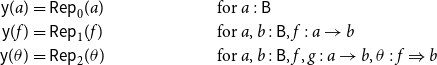 \begin{align*}\mathsf{y}(a) &= \mathsf{Rep}_0(a) && \mbox{for } a : \mathsf{B} \\\mathsf{y}(f) &= \mathsf{Rep}_1(f) && \mbox{for } a, b : \mathsf{B}, f : a \rightarrow b \\\mathsf{y}(\theta) &= \mathsf{Rep}_2(\theta) && \mbox{for } a, b : \mathsf{B}, f, g : a \rightarrow b, \theta : f \Rightarrow b\end{align*}
Problem 5.3 (Bicategorical Yoneda lemma) Given a locally univalent bicategory $\mathsf{B}$
, a pseudofunctor
$\mathsf{B}$
, a pseudofunctor $P : {\mathsf{B}^{\operatorname{\mathsf{{op}}}}} \rightarrow {\mathsf{Cat}}$
, and
$P : {\mathsf{B}^{\operatorname{\mathsf{{op}}}}} \rightarrow {\mathsf{Cat}}$
, and $a : \mathsf{B}$
, to construct an adjoint equivalence between the categories
$a : \mathsf{B}$
, to construct an adjoint equivalence between the categories $\underline{{\mathsf{Pseudo}(\mathsf{B}^{\operatorname{\mathsf{{op}}}}, \mathsf{Cat})}({\mathsf{y}(a)},{P})}$
and P(a).
$\underline{{\mathsf{Pseudo}(\mathsf{B}^{\operatorname{\mathsf{{op}}}}, \mathsf{Cat})}({\mathsf{y}(a)},{P})}$
and P(a).
Construction 5.4 for Problem 5.3; (bicategorical_yoneda_lemma). To construct this, we provide
(yoneda_to_presheaf) A functor F from
${\mathsf{y}(a)} \Rightarrow {P}$
to P(a);(presheaf_to_yoneda) A functor G from P(a) to
${\mathsf{y}(a)} \Rightarrow {P}$
;(yoneda_unit) A natural isomorphism from the identity to
$F \cdot G$
;(yoneda_counit) A natural isomorphism from
$G \cdot F$
to the identity.


We only discuss the data of the involved functors. The functor F sends pseudotransformations $\tau$
to
$\tau$
to $\tau(a)({\operatorname{id}}_1(a))$
and modifications m to
$\tau(a)({\operatorname{id}}_1(a))$
and modifications m to $m(a)({\operatorname{id}}_1(a))(a)$
. In the other direction, G sends objects
$m(a)({\operatorname{id}}_1(a))(a)$
. In the other direction, G sends objects $z : P(a)$
to the pseudotransformation whose components are P(f)(z) with
$z : P(a)$
to the pseudotransformation whose components are P(f)(z) with $b : \mathsf{B}^{\operatorname{\mathsf{{op}}}}$
and
$b : \mathsf{B}^{\operatorname{\mathsf{{op}}}}$
and $f : b \rightarrow a$
.
$f : b \rightarrow a$
.
Now let us use the bicategorical Yoneda lemma to construct for each locally univalent bicategory a weakly equivalent univalent bicategory. We follow the construction of the Rezk completion by Ahrens et al. (Reference Ahrens, Kapulkin and Shulman2015) and take the image of the Yoneda embedding to be the univalent completion.
First, we define weak equivalences of bicategories.
Definition 5.5. Let $\mathsf{B}$
and
$\mathsf{B}$
and $\mathsf{C}$
be bicategories and let
$\mathsf{C}$
be bicategories and let $F : \mathsf{B} \rightarrow \mathsf{C}$
be a pseudofunctor. We say
$F : \mathsf{B} \rightarrow \mathsf{C}$
be a pseudofunctor. We say
(local_equivalence) F is a local equivalence if for each
$x, y : \mathsf{B}$
the functor from
$\underline{{\mathsf{B}_1}({x},{y})}$
to
$\underline{{\mathsf{C}_1}({F(x)},{F(y)})}$
induced by F is an adjoint equivalence.(essentially_surjective) F is essentially surjective if for each
$y : \mathsf{C}$
there merely exists an
$x : \mathsf{B}$
and an adjoint equivalence from F(x) to y.(weak_equivalence) F is a weak equivalence if F is both a local equivalence and essentially surjective.


The notion of weak equivalence has already been studied in classical mathematics where, using the axiom of choice, it was shown to be equivalent to the usual notion of equivalence (Lack Reference Lack2010; Leinster Reference Leinster1998). However, these notions are generally not equivalent in a constructive setting, but we conjecture that they are for univalent bicategories.
Furthermore, the notion of weak equivalence can be weakened by requiring that the pseudofunctor only induces a weak equivalence of categories on the hom-categories. Such a weaker notion would be useful if one desires to find a univalent completion of arbitrary bicategories instead of just locally univalent ones. To do so, we anticipate a two-step process: first, a local completion, which embeds bicategories in locally univalent ones, followed by, second, the construction described in this section. More concretely, for any bicategory $\mathsf{B}$
we expect to be able to construct pseudofunctors as in the following diagram.
$\mathsf{B}$
we expect to be able to construct pseudofunctors as in the following diagram.
Here, $\mathcal{RC}_{\mathsf{loc}}(B)$
is a locally univalent bicategory, and
$\mathcal{RC}_{\mathsf{loc}}(B)$
is a locally univalent bicategory, and $\mathcal{RC}(B)$
is a univalent one. While the pseudofunctor
$\mathcal{RC}(B)$
is a univalent one. While the pseudofunctor ${{{\eta_{\mathsf{glob}}}}} : \mathcal{RC}_{\mathsf{loc}}(B) \to \mathcal{RC}(B)$
would be a weak equivalence according to Definition 5.5,
${{{\eta_{\mathsf{glob}}}}} : \mathcal{RC}_{\mathsf{loc}}(B) \to \mathcal{RC}(B)$
would be a weak equivalence according to Definition 5.5, ${{{\eta_{\mathsf{loc}}}}} : \mathsf{B} \to \mathcal{RC}_{\mathsf{loc}}(B)$
, would not be: locally, it consists of weak equivalences of categories instead of equivalences. Hence, the more general notion would thus be applicable if one is interested in the univalent completion of arbitrary bicategories. We expect such a local completion
${{{\eta_{\mathsf{loc}}}}} : \mathsf{B} \to \mathcal{RC}_{\mathsf{loc}}(B)$
, would not be: locally, it consists of weak equivalences of categories instead of equivalences. Hence, the more general notion would thus be applicable if one is interested in the univalent completion of arbitrary bicategories. We expect such a local completion ${{{\eta_{\mathsf{loc}}}}} : B \to \mathcal{RC}_{\mathsf{loc}}(B)$
can be constructed by taking the Rezk completion of every hom-category, and since that only yields a weak equivalence of categories, the resulting pseudofunctor is not locally an equivalence. However, we only consider the second step in this paper and leave the construction of
${{{\eta_{\mathsf{loc}}}}} : B \to \mathcal{RC}_{\mathsf{loc}}(B)$
can be constructed by taking the Rezk completion of every hom-category, and since that only yields a weak equivalence of categories, the resulting pseudofunctor is not locally an equivalence. However, we only consider the second step in this paper and leave the construction of ${{{\eta_{\mathsf{loc}}}}} : \mathsf{B} \to \mathcal{RC}_{\mathsf{loc}}(B)$
as an open problem.
${{{\eta_{\mathsf{loc}}}}} : \mathsf{B} \to \mathcal{RC}_{\mathsf{loc}}(B)$
as an open problem.
Conjecture 5.6. For every bicategory $\mathsf{B},$
there is a locally univalent bicategory
$\mathsf{B},$
there is a locally univalent bicategory $\mathcal{RC}_{\mathsf{loc}}(B)$
and a pseudofunctor
$\mathcal{RC}_{\mathsf{loc}}(B)$
and a pseudofunctor ${{{\eta_{\mathsf{loc}}}}} : {\mathsf{B}} \rightarrow {\mathcal{RC}_{\mathsf{loc}}(B)}$
which is essentially surjective and locally a weak equivalence of categories.
${{{\eta_{\mathsf{loc}}}}} : {\mathsf{B}} \rightarrow {\mathcal{RC}_{\mathsf{loc}}(B)}$
which is essentially surjective and locally a weak equivalence of categories.
Weak equivalences between univalent categories are actually equivalences (Ahrens et al., Reference Ahrens, Kapulkin and Shulman2015, Lemma 6.8).We conjecture that the same is possible for bicategories.
Conjecture 5.7 Every weak equivalence between univalent bicategories is a biequivalence.
From the Yoneda lemma, we know that $\mathsf{y}$
is a local equivalence:
$\mathsf{y}$
is a local equivalence:
Corollary 5.8 (yoneda_mor_is_equivalence)) The pseudofunctor $\mathsf{y}$
is a local equivalence.
$\mathsf{y}$
is a local equivalence.
However, $\mathsf{y}$
is not essentially surjective: the bicategory
$\mathsf{y}$
is not essentially surjective: the bicategory $\mathsf{Pseudo}(\mathsf{B}^{\operatorname{\mathsf{{op}}}}, \mathsf{Cat})$
contains non-representable presheaves. To make
$\mathsf{Pseudo}(\mathsf{B}^{\operatorname{\mathsf{{op}}}}, \mathsf{Cat})$
contains non-representable presheaves. To make $\mathsf{y}$
essentially surjective, we restrict the bicategory of presheaves to the full image of the Yoneda embedding.
$\mathsf{y}$
essentially surjective, we restrict the bicategory of presheaves to the full image of the Yoneda embedding.
Definition 5.9 ((full_image)) Let $\mathsf{B}$
and
$\mathsf{B}$
and $\mathsf{C}$
be bicategories and let
$\mathsf{C}$
be bicategories and let $F : \mathsf{B} \rightarrow \mathsf{C}$
be a pseudofunctor. Then, the full image
$F : \mathsf{B} \rightarrow \mathsf{C}$
be a pseudofunctor. Then, the full image $\mathsf{im}(F)$
of F is the full subbicategory consisting of those objects c in
$\mathsf{im}(F)$
of F is the full subbicategory consisting of those objects c in $\mathsf{C}$
for which there merely exists
$\mathsf{C}$
for which there merely exists $b : \mathsf{B}$
such that
$b : \mathsf{B}$
such that $F(b) = c$
.
$F(b) = c$
.
Proposition 5.10 ((is_univalent_2_full_image)) If $\mathsf{C}$
is univalent, then so is the full image of
$\mathsf{C}$
is univalent, then so is the full image of $F : \mathsf{B} \rightarrow \mathsf{C}$
.
$F : \mathsf{B} \rightarrow \mathsf{C}$
.
Proof. Follows from Item 3 in Example 3.18.
Definition 5.11 (corestrict_full_image). Again let $\mathsf{B}$
and
$\mathsf{B}$
and $\mathsf{C}$
be bicategories and suppose we have a pseudofunctor
$\mathsf{C}$
be bicategories and suppose we have a pseudofunctor $F : \mathsf{B} \rightarrow \mathsf{C}$
. Then, we define the corestriction of F to be the pseudofunctor
$F : \mathsf{B} \rightarrow \mathsf{C}$
. Then, we define the corestriction of F to be the pseudofunctor $\overline{F} : {\mathsf{B}} \rightarrow {\mathsf{im}(F)}$
which sends b to F(b). The fact that F(b) is indeed in the image is witnessed by
$\overline{F} : {\mathsf{B}} \rightarrow {\mathsf{im}(F)}$
which sends b to F(b). The fact that F(b) is indeed in the image is witnessed by $|(b , \operatorname{\mathsf{{refl}}})|$
.
$|(b , \operatorname{\mathsf{{refl}}})|$
.
Now everything is in place to construct the desired embedding into a univalent bicategory.
Problem 5.12. For each locally univalent bicategory $\mathsf{B}$
, to construct a univalent bicategory
$\mathsf{B}$
, to construct a univalent bicategory $\mathcal{RC}(\mathsf{B})$
and a weak equivalence
$\mathcal{RC}(\mathsf{B})$
and a weak equivalence $F : {\mathsf{B}} \rightarrow {\mathcal{RC}(\mathsf{B})}$
.
$F : {\mathsf{B}} \rightarrow {\mathcal{RC}(\mathsf{B})}$
.
Construction 5.13 for Problem 5.12; (rezk_completion_2_0). We define $\mathcal{RC}(\mathsf{B})$
to be the image of the Yoneda embedding
$\mathcal{RC}(\mathsf{B})$
to be the image of the Yoneda embedding $\mathsf{y} : {\mathsf{B}} \rightarrow {\mathsf{Pseudo}(\mathsf{B}^{\operatorname{\mathsf{{op}}}}, \mathsf{Cat})}$
. Since the codomain of
$\mathsf{y} : {\mathsf{B}} \rightarrow {\mathsf{Pseudo}(\mathsf{B}^{\operatorname{\mathsf{{op}}}}, \mathsf{Cat})}$
. Since the codomain of $\mathsf{y}$
is univalent by Theorem 3.20, the image is univalent as well by Proposition 5.10. Note that the corestriction gives rise to a pseudofunctor
$\mathsf{y}$
is univalent by Theorem 3.20, the image is univalent as well by Proposition 5.10. Note that the corestriction gives rise to a pseudofunctor $\overline{\mathsf{y}} : {\mathsf{B}} \rightarrow {\mathcal{RC}(\mathsf{B})}$
. It is essentially surjective by construction. Furthermore,
$\overline{\mathsf{y}} : {\mathsf{B}} \rightarrow {\mathcal{RC}(\mathsf{B})}$
. It is essentially surjective by construction. Furthermore, $\mathsf{y}$
is a local equivalence by Corollary 5.8, and local equivalences are preserved by corestriction. Hence,
$\mathsf{y}$
is a local equivalence by Corollary 5.8, and local equivalences are preserved by corestriction. Hence, $\overline{\mathsf{y}}$
is indeed a weak equivalence.
$\overline{\mathsf{y}}$
is indeed a weak equivalence.
Note that Construction 5.13 raises universe levels: the bicategory $\mathcal{RC}(\mathsf{B})$
lives in a higher universe than B itself, for the same reasons as in the 1-categorical case (Ahrens et al. Reference Ahrens, Kapulkin and Shulman2015, Remark 8.6).
$\mathcal{RC}(\mathsf{B})$
lives in a higher universe than B itself, for the same reasons as in the 1-categorical case (Ahrens et al. Reference Ahrens, Kapulkin and Shulman2015, Remark 8.6).
6. Displayed Bicategories
Now let us study how to construct more complicated univalent bicategories. To that end, we introduce displayed bicategories, the bicategorical analog to the notion of displayed category developed by Ahrens and Lumsdaine (Reference Ahrens and Lumsdaine2019). A displayed (1-)category D over a given (base) category C consists of a family of objects over objects in C and a family of morphisms over morphisms in C together with suitable displayed operations of composition and identity. A category ${\textstyle \int_{{D}}{}}$
is then constructed, the objects and morphisms of which are pairs of objects and morphisms from C and D, respectively. Properties of
${\textstyle \int_{{D}}{}}$
is then constructed, the objects and morphisms of which are pairs of objects and morphisms from C and D, respectively. Properties of ${\textstyle \int_{{D}}{}}$
, in particular univalence, can be shown from analogous, but simpler, conditions on C and D.
${\textstyle \int_{{D}}{}}$
, in particular univalence, can be shown from analogous, but simpler, conditions on C and D.
A prototypical example is the following displayed category over $C:\equiv \mathsf{Set}$
: an object over a set X is a group structure on X, and a morphism over a function
$C:\equiv \mathsf{Set}$
: an object over a set X is a group structure on X, and a morphism over a function $f : X \to X'$
from group structure G (on X) to group structure G’ (on X’) is a proof of the fact that f is compatible with G and G’. The total category is the category of groups, and its univalence follows from univalence of
$f : X \to X'$
from group structure G (on X) to group structure G’ (on X’) is a proof of the fact that f is compatible with G and G’. The total category is the category of groups, and its univalence follows from univalence of $\mathsf{Set}$
and a univalence property of the displayed data.
$\mathsf{Set}$
and a univalence property of the displayed data.
Just like in 1-category theory, many examples of bicategories are obtained by endowing previously considered bicategories with additional structure. An example is the bicategory of pointed 1-types in $\operatorname{\textsf{U}}$
. The objects in this bicategory are pairs of a 1-type A and an inhabitant
$\operatorname{\textsf{U}}$
. The objects in this bicategory are pairs of a 1-type A and an inhabitant $a : A$
. The morphisms are pairs of a morphism f of 1-types and a path witnessing that f preserves the selected points. Similarly, the 2-cells are pairs of a homotopy p and a proof that this p commutes with the point preservation proofs. Thus, this bicategory is obtained from
$a : A$
. The morphisms are pairs of a morphism f of 1-types and a path witnessing that f preserves the selected points. Similarly, the 2-cells are pairs of a homotopy p and a proof that this p commutes with the point preservation proofs. Thus, this bicategory is obtained from $\mbox{1-}\mathsf{Type}_{\operatorname{\textsf{U}}}$
by endowing the cells on each level with additional structure.
$\mbox{1-}\mathsf{Type}_{\operatorname{\textsf{U}}}$
by endowing the cells on each level with additional structure.
Of course, the structure should be added in such a way that we are guaranteed to obtain a bicategory at the end. Now let us give the formal definition of displayed bicategories.
Definition 6.1 ((disp-bicat)) Given a bicategory $\mathsf{B}$
, a displayed bicategory
$\mathsf{B}$
, a displayed bicategory $\mathsf{D}$
over
$\mathsf{D}$
over $\mathsf{B}$
is given by data analogous to that of a bicategory, to which the numbering refers:
$\mathsf{B}$
is given by data analogous to that of a bicategory, to which the numbering refers:
-
1. for each
$a : \mathsf{B}_0$
a type
${{{{{\mathsf{D}}}_{a}}}}$
of displayed 0-cells over a; -
2. for each
$f : a \rightarrow b$
in
$\mathsf{B}$
and
$\bar{a} : {{{{\mathsf{D}}_{a}}}} , \bar{b} : {{{{\mathsf{D}}_{b}}}}$
a type
${\bar{a}} \xrightarrow{f} {\bar{b}}$
of displayed 1-cells over f; -
3. for each
$\theta : f \Rightarrow g$
in
$\mathsf{B}$
,
$\bar{f} : {\bar{a}} \xrightarrow{f} {\bar{b}}$
and
$\bar{g} : {\bar{a}} \xrightarrow{g} {\bar{b}}$
a set of displayed 2-cells over
$\theta$
and dependent versions of operations and laws from Definition 2.1, which are -
4. for each
$a : \mathsf{B}_0$
and
$\bar{a} : {{{{\mathsf{D}}_{a}}}}$
, we have
$\operatorname{id}_1(\bar{a}) : {\bar{a}} \xrightarrow{{\operatorname{id}_1\!(a)}} {\bar{a}}$
; -
5. for all 1-cells
$f : a \rightarrow b$
,
$g : b \rightarrow c$
, and displayed 1-cells
$\bar{f} : {\bar{a}} \xrightarrow{f} {\bar{b}}$
and
$\bar{g} : {\bar{b}} \xrightarrow{\bar{c}} {\bar{c}}$
, we have a displayed 1-cell
$\bar{f} \cdot \bar{g} : {\bar{a}} \xrightarrow{{f \cdot g}} {\bar{c}}$
; -
6. for all
$f : \mathsf{B}_1(a,b)$
,
$\bar{a} : {{{{\mathsf{D}}_{a}}}}$
,
$\bar{b} : {{{{\mathsf{D}}_{b}}}}$
, and
$\bar{f} : {\bar{a}} \xrightarrow{f} {\bar{b}}$
, we have ; -
7. for 2-cells
$\theta : f \Rightarrow g$
and
$\gamma : g \Rightarrow h$
, and displayed 2-cells and
$\bar{\gamma} : {\bar{g}} \xrightarrow{\gamma} {\bar{h}}$
, we have a displayed 2-cell . -
8. for each displayed 1-cell
$\bar{f} : {\bar{a}} \xrightarrow{f} {\bar{b}}$
and each displayed 2-cell , we have a displayed 2-cell ; -
9. for each displayed 1-cell
$\bar{h} : {\bar{b}} \xrightarrow{h} {\bar{c}}$
and each displayed 2-cell , we have a displayed 2-cell ; -
10. for each
$\bar{f} : {\bar{a}} \xrightarrow{f} {\bar{b}}$
, we have displayed 2-cells and ; -
11. for each
$\bar{f} : {\bar{a}} \xrightarrow{f} {\bar{b}}$
, displayed 2-cells and ; -
12. for each
, , and , we have displayed 2-cells and .


Note that we use the same notation for the displayed and the non-displayed operations.
These operations are subject to laws, which are derived systematically from the non-displayed version. Just as for displayed 1-categories, the laws of displayed bicategories are heterogeneous, because they are transported along the analogous law in the base bicategory. For instance, the displayed left-unitary law for identity reads as $\operatorname{id}_2\!(\bar{f}) \bullet \bar{\theta} =_e \bar{\theta}$
, where e is the corresponding identity of item 13 in Definition 2.1.
$\operatorname{id}_2\!(\bar{f}) \bullet \bar{\theta} =_e \bar{\theta}$
, where e is the corresponding identity of item 13 in Definition 2.1.
-
13.
$\operatorname{id}_2\!(f) \bullet \theta =_* \theta, \quad \theta \bullet \operatorname{id}_2\!(g) =_* \theta, \quad \theta \bullet (\gamma \bullet \tau) =_* (\theta \bullet \gamma) \bullet \tau$
; -
14.
$f \vartriangleleft ({\operatorname{id}}_2 g) =_* \operatorname{id}_2\!(f \cdot g), \quad f \vartriangleleft (\theta \bullet \gamma) =_* (f \vartriangleleft \theta) \bullet (f \vartriangleleft \gamma)$
; -
15.
$({\operatorname{id}}_2 f) \vartriangleright g =_* \operatorname{id}_2\!(f \cdot g), \quad (\theta \bullet \gamma) \vartriangleright g =_* (\theta \vartriangleright g) \bullet (\gamma \vartriangleright g)$
; -
16.
$({\operatorname{id}}_1(a) \vartriangleleft \theta) \bullet \lambda(g) =_* \lambda(f) \bullet \theta$
; -
17.
$(\theta \vartriangleright \operatorname{id}_1\!(b)) \bullet \rho(g) =_* \rho(f) \bullet \theta$
; -
18.
$(f \vartriangleleft (g \vartriangleleft \theta)) \bullet \alpha(f, g, i) =_* \alpha(f,g,h) \bullet ((f \cdot g) \vartriangleleft \theta)$
; -
19.
$(f \vartriangleleft (\theta \vartriangleright i)) \bullet \alpha(f,h,i) =_* \alpha(f,g,i) \bullet ((f \vartriangleleft \theta) \vartriangleright i)$
; -
20.
$(\theta \vartriangleright (h \cdot i)) \bullet \alpha(g,h,i) =_* \alpha(f,h,i) \bullet ((\theta \vartriangleright h) \vartriangleright i)$
; -
21.
$\lambda(f) \bullet \lambda(f)^{-1} =_* \operatorname{id}_2\!({\operatorname{id}}_1(a) \cdot f), \quad \lambda(f)^{-1} \bullet \lambda(f) =_* \operatorname{id}_2\!(f)$
; -
22.
$\rho(f) \bullet \rho(f)^{-1} =_* \operatorname{id}_2\!(f \cdot \operatorname{id}_1\!(b)), \quad \rho(f)^{-1} \bullet \rho(f) =_* \operatorname{id}_2\!(f)$
; -
23.
$\alpha(f,g,h) \bullet \alpha(f,g,h)^{-1} =_* \operatorname{id}_2\!(f \cdot (g \cdot h)), \quad \alpha(f,g,h)^{-1} \bullet \alpha(f,g,h) =_* \operatorname{id}_2\!((f \cdot g) \cdot h)$
; -
24.
$\alpha(f, \operatorname{id}_1\!(b),g) \bullet (\rho(f) \vartriangleright g) =_* f \vartriangleleft \lambda(f)$
; -
25.
$\alpha(f,g,h \cdot i) \bullet \alpha(f \cdot g, h, i) =_* (f \vartriangleleft \alpha(g,h,i)) \bullet \alpha(f,g \cdot h, i) \bullet (\alpha(f,g,h) \vartriangleright i)$
.


The purpose of displayed bicategories is to give rise to a total bicategory together with a projection pseudofunctor. They are defined as follows:
Definition 6.2 (total_bicat). Given a displayed bicategory $\mathsf{D}$
over a bicategory
$\mathsf{D}$
over a bicategory $\mathsf{B}$
, we form the total bicategory
$\mathsf{B}$
, we form the total bicategory ${\textstyle \int_{\mathsf{D}}{}}$
(or
${\textstyle \int_{\mathsf{D}}{}}$
(or ${\textstyle \int_{[\mathsf{B}]}{{\mathsf{D}}}}$
) which has:
${\textstyle \int_{[\mathsf{B}]}{{\mathsf{D}}}}$
) which has:
-
(1) as 0-cells tuples
$(a, \bar{a})$
, where
$a : \mathsf{B}$
and
$\bar{a} : {{{{\mathsf{D}}_{a}}}}$
; -
(2) as 1-cells tuples
$(f, \bar{f}) : (a,\bar{a}) \rightarrow (b,\bar{b})$
, where
$f : a \rightarrow b$
and
$\bar{f} : {\bar{a}} \xrightarrow{f} {\bar{b}}$
; -
(3) as 2-cells tuples
$(\theta, \bar{\theta}) : (f, \bar{f}) \Rightarrow (g, \bar{g})$
, where
$\theta : f \Rightarrow g$
and .


We also have a projection pseudofunctor $\pi_D : {{\textstyle \int_{{D}}{}}} \rightarrow {\mathsf{B}}$
.
$\pi_D : {{\textstyle \int_{{D}}{}}} \rightarrow {\mathsf{B}}$
.
As mentioned before, the bicategory of pointed 1-types is the total bicategory of the following displayed bicategory.
Example 6.3 (p1types_disp, Example 3.18, Item 2 cont’d). Given a universe $\operatorname{\textsf{U}}$
, we build a displayed bicategory of pointed 1-types over the base bicategory of 1-types in
$\operatorname{\textsf{U}}$
, we build a displayed bicategory of pointed 1-types over the base bicategory of 1-types in $\operatorname{\textsf{U}}$
(Example 2.7).
$\operatorname{\textsf{U}}$
(Example 2.7).
For 1-type A in
$\operatorname{\textsf{U}}$
, the objects over A are inhabitants of A.For
$f : A \rightarrow B$
with A, B 1-types in
$\operatorname{\textsf{U}}$
, the displayed 1-cells over f from a to b are paths
$f(a) = b$
.Given two functions
$f, g : A \rightarrow B$
, a homotopy
$p : f \sim g$
, two points
$a : A$
and
$b : B$
, and paths
$q_f : f(a) = b$
and
$q_g : g(a) = b$
, the 2-cells over p are paths
$q_f = p(a) \bullet q_g$
.


The bicategory of pointed 1-types is the total bicategory of this displayed bicategory.
Example 6.4 ((pgrpds)) We define a displayed bicategory of pointed groupoids over the base bicategory $\mathsf{Grpd}$
of groupoids.
$\mathsf{Grpd}$
of groupoids.
For a groupoid G, the objects over G are objects of G.
For a functor
$F : G_1 \rightarrow G_2$
between groupoids
$G_1$
and
$G_2$
, the displayed 1-cells over F from x to y are isomorphisms
$F(a) \cong b$
.Given two functors
$F_1, F_2 : G_1 \rightarrow G_2$
, a natural transformation
$n : F_1 \Rightarrow F_2$
, two points
$x : G_1$
and
$y : G_2$
, and isomorphisms
$q_1 : F_1(x) \cong y$
and
$q_2 : F_2(x) = y$
, the displayed 2-cells over n are paths
$p(a) \bullet q_g = q_f$
.


The bicategory of pointed groupoids is the total bicategory of this displayed bicategory.
Example 6.5 ((disp-fullsubbicat)) Given a bicategory $\mathsf{B}$
and a predicate on 0-cells
$\mathsf{B}$
and a predicate on 0-cells $P : \mathsf{B}_0 \to \operatorname{\textsf{hProp}}$
, define a displayed bicategory
$P : \mathsf{B}_0 \to \operatorname{\textsf{hProp}}$
, define a displayed bicategory $\mathsf{D}$
over
$\mathsf{D}$
over $\mathsf{B}$
such that
$\mathsf{B}$
such that ${{{{\mathsf{D}}_{x}}}} :\equiv P(x)$
, and the types of displayed 1-cells and 2-cells are the unit type. The total bicategory of
${{{{\mathsf{D}}_{x}}}} :\equiv P(x)$
, and the types of displayed 1-cells and 2-cells are the unit type. The total bicategory of $\mathsf{D}$
provides a formal construction of the full subbicategory of
$\mathsf{D}$
provides a formal construction of the full subbicategory of $\mathsf{B}$
with cells satisfying P introduced in Definition 2.10. In particular, a 1-cell in the total bicategory of
$\mathsf{B}$
with cells satisfying P introduced in Definition 2.10. In particular, a 1-cell in the total bicategory of $\mathsf{D}$
is a pair consisting of a 1-cell from
$\mathsf{D}$
is a pair consisting of a 1-cell from $\mathsf{B}$
and the unique inhabitant of the unit type. Similarly for 2-cells.
$\mathsf{B}$
and the unique inhabitant of the unit type. Similarly for 2-cells.
We end this section presenting several general constructions of displayed bicategories.
Definition 6.6 ((Various constructions of displayed bicategories))
-
(1) (disp_dirprod_bicat) Given displayed bicategories
$\mathsf{D}_1$
and
$\mathsf{D}_2$
over a bicategory
$\mathsf{B}$
, we construct the product
$\mathsf{D}_1 \times \mathsf{D}_2$
over
$\mathsf{B}$
. The 0-cells, 1-cells, and 2-cells are pairs of 0-cells, 1-cells, and 2-cells, respectively. -
(2) (sigma_bicat) Given a displayed bicategory
$\mathsf{D}$
over a base
$\mathsf{B}$
and a displayed bicategory
$\mathsf{E}$
over
${\textstyle \int_{\mathsf{D}}{}}$
, we construct the sigma displayed bicategory
${\sum_{[\mathsf{D}]}{{\mathsf{E}}}}$
over
$\mathsf{B}$
as follows. The objects over
$a : \mathsf{B}$
are pairs
$(\bar{a}, e)$
, where
$\bar{a} : {{{{\mathsf{D}}_{a}}}}$
and
$e : {{{{{\mathsf{E}}}_{{(a,\bar{a})}}}}}$
, the morphisms over
$f : {a} \rightarrow {b}$
from
$(\bar{a}, e)$
to
$(\bar{b}, e')$
are pairs
$(\bar{f}, \varphi)$
, where
$\bar{f} : {\bar{a}} \xrightarrow{f} {\bar{b}}$
and
$\varphi : {e} \xrightarrow{{(f, \bar{f})}} {e'}$
, and similarly for 2-cells. -
(3) (trivial_displayed_bicat) Every bicategory
$\mathsf{D}$
is, in a trivial way, a displayed bicategory over any other bicategory
$\mathsf{B}$
. Its total bicategory is the direct product
$\mathsf{B} \times \mathsf{D}$
. -
(4) (disp_cell_unit_bicat) We say a displayed bicategory
$\mathsf{D}$
over
$\mathsf{B}$
is locally chaotic if, for each
$\alpha : f \Rightarrow g$
and
$\bar{f} : {\bar{a}} \xrightarrow{f} {\bar{b}}$
and
$\bar{g} : {\bar{a}} \xrightarrow{g} {\bar{b}}$
, the type is contractible. Let
$\mathsf{B}$
be a bicategory and suppose we have -
− for each object a in
$\mathsf{B}$
a type
${{{{\mathsf{D}}_{b}}}}$
of displayed 0-cells; -
− for each 1-cell
$f : a \rightarrow b$
in
$\mathsf{B}$
and for each
$\bar{a} : {{{{\mathsf{D}}_{a}}}}, \bar{b} : {{{{\mathsf{D}}_{b}}}}$
a type
${\bar{a}} \xrightarrow{f} {\bar{b}}$
of displayed 1-cells; -
− displayed 1-identities
$\operatorname{id}_1$
and compositions
$(\cdot)$
of displayed 1-cells as in Definition 6.1. Then we have an associated locally chaotic displayed bicategory
$\hat{\mathsf{D}}$
over
$\mathsf{B}$
by stipulating that the types of 2-cells are the unit type. Note that this construction essentially gives a way of obtaining a displayed bicategory from the data of a displayed category (Ahrens and Lumsdaine Reference Ahrens and Lumsdaine2019, Def. 3.1, Items 1–4).


Now let us discuss two more examples of bicategories obtained from displayed bicategories: firstly, monads internal to an arbitrary bicategory and secondly, Kleisli triples. In Construction 8.14, we construct a biequivalence between the bicategory of Kleisli triples and the bicategory of monads internal to $\mathsf{Cat}$
.
$\mathsf{Cat}$
.
Definition 6.7 ((monad)) Let $\mathsf{B}$
be a bicategory. Then, we define a displayed bicategory
$\mathsf{B}$
be a bicategory. Then, we define a displayed bicategory $\mathsf{M}(\mathsf{B})$
over
$\mathsf{M}(\mathsf{B})$
over $\mathsf{B}$
such that
$\mathsf{B}$
such that
The displayed objects over
$a : \mathsf{B}$
are monad structures on a. A monad structure on a consists of a 1-cell
$m_a : a \rightarrow a$
and 2-cells
$\eta_a : \operatorname{id}_1\!(a) \Rightarrow m$
and
$\mu_a : m \cdot m \Rightarrow m$
such that the following diagrams commute The displayed 1-cells over
$f : a \rightarrow b$
from
$(m_a, \eta_a, \mu_a)$
to
$(m_b, \eta_b, \mu_b)$
consist of invertible 2-cells
$n_f : m_a \cdot f \Rightarrow f \cdot m_b$
such that the following two diagrams commute The displayed 2-cells over
$x : f \Rightarrow g$
from
$n_f$
to
$n_g$
are proofs that the following diagrams commute


The total bicategory of $\mathsf{M}(\mathsf{B})$
is the bicategory of monads internal to
$\mathsf{M}(\mathsf{B})$
is the bicategory of monads internal to $\mathsf{B}$
.
$\mathsf{B}$
.
Next, we define a bicategory of Kleisli triples, also known as extension systems (Marmolejo and Wood Reference Marmolejo and Wood2010).
Definition 6.8 ((kleisli_triple-disp-bicat)) We define a displayed bicategory $\mathsf{K}$
over
$\mathsf{K}$
over $\mathsf{Cat}$
such that
$\mathsf{Cat}$
such that
The displayed objects over C are Kleisli triples over C. These consist of a function
$M : C_0 \rightarrow C_0$
, for each
$a : C$
an arrow
$\eta(a) : a \rightarrow M(a)$
, and for each arrow
$f : a \rightarrow M(b)$
, an arrow
$f^* : M(a) \rightarrow M(b)$
such that the usual laws hold.The displayed 1-cells over a functor
$F : C \rightarrow D$
from
$M_C$
to
$M_D$
consists of isomorphisms
$F_M$
from
$M_D(F(a))$
to
$F(M_C(a))$
for each
$a : C_0$
such that the usual laws hold.The displayed 2-cells over
$n : F \Rightarrow G$
from
$F_M$
to
$G_M$
are equalities
\begin{equation*} F_M(a) \cdot n(M_C(a)) = M_D(n(a)) \cdot G_M(a). \end{equation*}


The total bicategory of $\mathsf{K}$
is the bicategory of Kleisli triples.
$\mathsf{K}$
is the bicategory of Kleisli triples.
7. Displayed Univalence
Given a bicategory $\mathsf{B}$
and a displayed bicategory
$\mathsf{B}$
and a displayed bicategory $\mathsf{D}$
over
$\mathsf{D}$
over $\mathsf{B}$
, our goal is to prove the univalence of
$\mathsf{B}$
, our goal is to prove the univalence of ${\textstyle \int_{\mathsf{D}}{}}$
from conditions on
${\textstyle \int_{\mathsf{D}}{}}$
from conditions on $\mathsf{B}$
and
$\mathsf{B}$
and $\mathsf{D}$
. For that, we develop the notion of univalent displayed bicategories. We start by defining displayed versions of invertible 2-cells.
$\mathsf{D}$
. For that, we develop the notion of univalent displayed bicategories. We start by defining displayed versions of invertible 2-cells.
Definition 7.1 ((is_disp_invertible_2cell)) Given are a bicategory $\mathsf{B}$
and a displayed bicategory
$\mathsf{B}$
and a displayed bicategory $\mathsf{D}$
over
$\mathsf{D}$
over $\mathsf{B}$
. Suppose we have objects
$\mathsf{B}$
. Suppose we have objects $a, b : \mathsf{B}_0$
, two 1-cells
$a, b : \mathsf{B}_0$
, two 1-cells $f, g : \mathsf{B}_1(a,b)$
, and an invertible 2-cell
$f, g : \mathsf{B}_1(a,b)$
, and an invertible 2-cell $\theta : \mathsf{B}_2(f,g)$
. Suppose that we also have
$\theta : \mathsf{B}_2(f,g)$
. Suppose that we also have $\bar{a} : {{{{D}_{a}}}}$
,
$\bar{a} : {{{{D}_{a}}}}$
, $\bar{b} : {{{{D}_{b}}}}$
,
$\bar{b} : {{{{D}_{b}}}}$
, $\bar{f} : {\bar{a}} \xrightarrow{f} {\bar{b}}$
,
$\bar{f} : {\bar{a}} \xrightarrow{f} {\bar{b}}$
, $\bar{g} : {\bar{a}} \xrightarrow{g} {\bar{b}}$
, and
$\bar{g} : {\bar{a}} \xrightarrow{g} {\bar{b}}$
, and ![]() . Then, we say
. Then, we say $\bar{\theta}$
is invertible if we have
$\bar{\theta}$
is invertible if we have ![]() such that
such that $\bar{\theta} \bullet \bar{\gamma}$
and
$\bar{\theta} \bullet \bar{\gamma}$
and $\bar{\gamma} \bullet \bar{\theta}$
are identities modulo transport over the corresponding identity laws of
$\bar{\gamma} \bullet \bar{\theta}$
are identities modulo transport over the corresponding identity laws of $\theta$
.
$\theta$
.
A displayed invertible 2-cell over $\theta$
, where
$\theta$
, where $\theta$
is an invertible 2-cell, is a pair of a displayed 2-cell
$\theta$
is an invertible 2-cell, is a pair of a displayed 2-cell $\bar{\theta}$
over
$\bar{\theta}$
over $\theta$
and a proof that
$\theta$
and a proof that $\bar{\theta}$
is invertible. The type of displayed invertible 2-cells from
$\bar{\theta}$
is invertible. The type of displayed invertible 2-cells from $\bar{f}$
to
$\bar{f}$
to $\bar{g}$
over
$\bar{g}$
over $\theta$
is denoted by
$\theta$
is denoted by ${{{ {{\bar{f}}} \cong_{{\theta}} {{\bar{g}}} }}}$
.
${{{ {{\bar{f}}} \cong_{{\theta}} {{\bar{g}}} }}}$
.
Being a displayed invertible 2-cell is a proposition and the displayed 2-cell $\operatorname{id}_2\!(\bar{f})$
over
$\operatorname{id}_2\!(\bar{f})$
over $\operatorname{id}_2\!(f)$
is invertible. Next, we define displayed adjoint equivalences.
$\operatorname{id}_2\!(f)$
is invertible. Next, we define displayed adjoint equivalences.
Definition 7.2 ((disp-left-adjoint-equivalence)) Given are a bicategory $\mathsf{B}$
and a displayed bicategory
$\mathsf{B}$
and a displayed bicategory $\mathsf{D}$
over
$\mathsf{D}$
over $\mathsf{B}$
. Suppose we have objects
$\mathsf{B}$
. Suppose we have objects $a, b : \mathsf{B}_0$
and a 1-cell
$a, b : \mathsf{B}_0$
and a 1-cell $f : \mathsf{B}_1(a,b)$
together with an adjoint equivalence structure A on f. We write r,
$f : \mathsf{B}_1(a,b)$
together with an adjoint equivalence structure A on f. We write r, $\eta$
,
$\eta$
, $\varepsilon$
for the right adjoint, unit, and counit of f respectively. Furthermore, suppose that we have
$\varepsilon$
for the right adjoint, unit, and counit of f respectively. Furthermore, suppose that we have $\bar{a} : {{{{\mathsf{D}}_{a}}}}$
,
$\bar{a} : {{{{\mathsf{D}}_{a}}}}$
, $\bar{b} : {{{{\mathsf{D}}_{b}}}}$
, and
$\bar{b} : {{{{\mathsf{D}}_{b}}}}$
, and $\bar{f} : {\bar{a}} \xrightarrow{f} {\bar{b}}$
. A displayed adjoint equivalence structure on
$\bar{f} : {\bar{a}} \xrightarrow{f} {\bar{b}}$
. A displayed adjoint equivalence structure on $\bar{f}$
consists of
$\bar{f}$
consists of
A displayed 1-cell
$\bar{r} : {\bar{b}} \xrightarrow{{r}} {\bar{a}}$
;An invertible displayed 2-cell
;An invertible displayed 2-cell
.

In addition, two laws reminiscent of those in Definition 2.5 need to be satisfied.
A displayed adjoint equivalence over the adjoint equivalence A is a pair of a displayed 1-cell $\bar{f}$
over f together with a displayed adjoint equivalence structure on
$\bar{f}$
over f together with a displayed adjoint equivalence structure on $\bar{f}$
. The type of displayed adjoint equivalences from
$\bar{f}$
. The type of displayed adjoint equivalences from $\bar{a}$
to
$\bar{a}$
to $\bar{b}$
over f is denoted by
$\bar{b}$
over f is denoted by ${{{ {{\bar{a}}} \simeq_{{f}} {{\bar{b}}} }}}$
.
${{{ {{\bar{a}}} \simeq_{{f}} {{\bar{b}}} }}}$
.
The displayed 1-cell $\operatorname{id}_1\!(\bar{a})$
is a displayed adjoint equivalence over
$\operatorname{id}_1\!(\bar{a})$
is a displayed adjoint equivalence over $\operatorname{id}_1\!(a)$
.
$\operatorname{id}_1\!(a)$
.
Using these definitions, we define univalence of displayed bicategories similarly to univalence for ordinary bicategories. Again we separate it in a local and global condition.
Definition 7.3 ((DispUnivalence)) Let $\mathsf{D}$
be a displayed bicategory over
$\mathsf{D}$
be a displayed bicategory over $\mathsf{B}$
.
$\mathsf{B}$
.
-
(1) Let
$a, b : \mathsf{B}$
, and
$\bar{a} : {{{{\mathsf{D}}_{a}}}}, \bar{b} : {{{{\mathsf{D}}_{b}}}}$
. Let
$f, g : {a} \rightarrow {b}$
, let
$p : f = g$
, and let
$\bar{f}$
and
$\bar{g}$
be displayed morphisms over f and g respectively. Then we define a function sending
\begin{equation*} \mathsf{disp\_idtoiso}^{2,1}_{p,\bar{f},\bar{g}} : \bar{f} =_{[p]} \bar{g} \rightarrow {{{ {{\bar{f}}} \cong_{{\mathsf{idtoiso}^{2,1}_{f,g}(p)}} {{\bar{g}}} }}} \end{equation*}
$\operatorname{\mathsf{{refl}}}$
to the identity displayed isomorphism. We say that
$\mathsf{D}$
is locally univalent if the function
$\mathsf{disp\_idtoiso}^{2,1}_{p,\bar{f},\bar{g}}$
is an equivalence for each p,
$\bar{f}$
, and
$\bar{g}$
.
-
(2) Let
$a, b : \mathsf{B}$
, and
$\bar{a} : {{{{\mathsf{D}}_{a}}}}, \bar{b} : {{{{\mathsf{D}}_{b}}}}$
. Given
$p : a = b$
, we define a function sending
\begin{equation*}\mathsf{disp\_idtoiso}^{2,0}_{p,\bar{a},\bar{b}} : \bar{a} =_{[p]} \bar{b} \rightarrow {{{ {{\bar{a}}} \simeq_{{\mathsf{idtoiso}^{2,0}_{a,b}(p)}} {{\bar{b}}} }}}\end{equation*}
$\operatorname{\mathsf{{refl}}}$
to the identity displayed adjoint equivalence. We say that
$\mathsf{D}$
is globally univalent if the function
$\mathsf{disp\_idtoiso}^{2,0}_{p,\bar{a},\bar{b}}$
is an equivalence for each p,
$\bar{a}$
, and
$\bar{b}$
.
-
(3) (disp_univalent_2) We call
$\mathsf{D}$
univalent if it is both locally and globally univalent.


The following result states that univalence of the total bicategory can be proved from univalence of the base and of the displayed part. This is the bicategorical version of the analogous result for 1-categories shown by Ahrens and Lumsdaine (Reference Ahrens and Lumsdaine2019, Theorem 7.4), which in turn generalizes the Structure Identity Principle (Univalent Foundations Program 2013, Theorem 9.8.2).
Theorem 7.4 ((total_is_univalent_2)) Let $\mathsf{B}$
be a bicategory and let
$\mathsf{B}$
be a bicategory and let $\mathsf{D}$
be a displayed bicategory over
$\mathsf{D}$
be a displayed bicategory over $\mathsf{B}$
. Then
$\mathsf{B}$
. Then
-
(1)
${\textstyle \int_{\mathsf{D}}{}}$
is locally univalent if
$\mathsf{B}$
is locally univalent and
$\mathsf{D}$
is locally univalent; -
(2)
${\textstyle \int_{\mathsf{D}}{}}$
is globally univalent if
$\mathsf{B}$
is globally univalent and
$\mathsf{D}$
is globally univalent.


Proof The main idea behind the proof is to characterize invertible 2-cells in the total bicategory as pairs of an invertible 2-cell p in the base bicategory and a displayed invertible 2-cell over p. Concretely, for the local univalence of $\mathsf{D}$
, we factor
$\mathsf{D}$
, we factor $\mathsf{idtoiso}^{2,1}$
as a composition of the following equivalences:
$\mathsf{idtoiso}^{2,1}$
as a composition of the following equivalences:
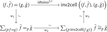
The function $w_1$
is just a characterization of paths in a sigma type. The function
$w_1$
is just a characterization of paths in a sigma type. The function $w_2$
turns equalities into (displayed) invertible 2-cells, and it is an equivalence by local univalence of
$w_2$
turns equalities into (displayed) invertible 2-cells, and it is an equivalence by local univalence of $\mathsf{B}$
and displayed local univalence of
$\mathsf{B}$
and displayed local univalence of $\mathsf{D}$
. Finally, the function
$\mathsf{D}$
. Finally, the function $w_3$
characterizes invertible 2-cells in the total bicategory.
$w_3$
characterizes invertible 2-cells in the total bicategory.
The proof is similar in the case of global univalence. The most important step is the characterization of adjoint equivalences in the total bicategory.
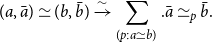 \begin{equation*}(a,\bar{a}) \simeq (b, \bar{b}) \xrightarrow{\sim}\sum_{(p : a \simeq b)} . {{{ {{\bar{a}}} \simeq_{{p}} {{\bar{b}}} }}}.\end{equation*}
To check displayed univalence, it suffices to prove the condition in the case where p is reflexivity. This step, done by path induction, simplifies some proofs of displayed univalence.
Proposition 7.5 Given a displayed bicategory $\mathsf{D}$
over
$\mathsf{D}$
over $\mathsf{B}$
, then
$\mathsf{B}$
, then $\mathsf{D}$
is univalent if the following functions are equivalences:
$\mathsf{D}$
is univalent if the following functions are equivalences:
(fiberwise_local_univalent_is_univalent_2_1)
\begin{equation*} \mathsf{disp\_idtoiso}^{2,1}_{\operatorname{\mathsf{{refl}}}(f),\bar{f},\overline{f'}} : \bar{f} = \overline{f'} \rightarrow {{{ {{\bar{f}}} \cong_{{\operatorname{id}_2\!(f)}} {{\overline{f'}}} }}} \end{equation*}
(fiberwise_univalent_2_0_to_disp_univalent_2_0)
\begin{equation*} \mathsf{disp\_idtoiso}^{2,0}_{\operatorname{\mathsf{{refl}}}(a),\bar{a},\overline{a'}} : \bar{a} = \overline{a'} \rightarrow {{{ {{\bar{a}}} \simeq_{{\operatorname{id}_1\!(a)}} {{\overline{a'}}} }}} \end{equation*}


Now, we establish the univalence of several examples.
Example 7.6 The following bicategories and displayed bicategories are univalent:
-
(1) The category of pointed 1-types (see Example 6.3) is univalent (p1types_univalent_2).
-
(2) The full subbicategory (see Definition 2.10) of a univalent bicategory is univalent (is_univalent_2_fullsubbicat).
-
(3) The product of univalent displayed bicategories (Definition 6.6, Item 1) is univalent (is_univalent_2_dirprod_bicat).
For the sigma construction, we give two conditions for the univalence of the total bicategory. If we have univalent displayed bicategories $\mathsf{D}_1$
and
$\mathsf{D}_1$
and $\mathsf{D}_2$
over
$\mathsf{D}_2$
over $\mathsf{B}$
and
$\mathsf{B}$
and ${\textstyle \int_{{\mathsf{D}_1,}}{}}$
respectively, then we can either show the univalence of
${\textstyle \int_{{\mathsf{D}_1,}}{}}$
respectively, then we can either show the univalence of ${\textstyle \int_{{({\sum_{[\mathsf{D}_1]}{{\mathsf{D}_2}}})}}{}}$
directly or we can show the displayed univalence of
${\textstyle \int_{{({\sum_{[\mathsf{D}_1]}{{\mathsf{D}_2}}})}}{}}$
directly or we can show the displayed univalence of ${\sum_{[\mathsf{D}_1]}{{\mathsf{D}_2}}}$
. Note that the second property could be necessary as an intermediate step for proving the univalence of a more complicated bicategory. For the proof of displayed univalence of
${\sum_{[\mathsf{D}_1]}{{\mathsf{D}_2}}}$
. Note that the second property could be necessary as an intermediate step for proving the univalence of a more complicated bicategory. For the proof of displayed univalence of ${\sum_{[\mathsf{D}_1]}{{\mathsf{D}_2}}}$
, we need two assumptions on both displayed bicategories.
${\sum_{[\mathsf{D}_1]}{{\mathsf{D}_2}}}$
, we need two assumptions on both displayed bicategories.
Definition 7.7 (disp_locally_groupoid). A displayed bicategory is locally groupoidal if all its displayed 2-cells are invertible.
Definition 7.8 ((disp-2cells-isaprop)) A displayed bicategory $\mathsf{D}$
over a bicategory
$\mathsf{D}$
over a bicategory $\mathsf{B}$
is called locally propositional if the type
$\mathsf{B}$
is called locally propositional if the type ![]() of displayed 2-cells over
of displayed 2-cells over $\theta$
is a proposition.
$\theta$
is a proposition.
Proposition 7.9. Let $\mathsf{D}_1$
and
$\mathsf{D}_1$
and $\mathsf{D}_2$
be univalent displayed bicategories over univalent bicategories
$\mathsf{D}_2$
be univalent displayed bicategories over univalent bicategories $\mathsf{B}$
and
$\mathsf{B}$
and ${\textstyle \int_{\mathsf{D}_1}{}}$
respectively.
${\textstyle \int_{\mathsf{D}_1}{}}$
respectively.
-
(1) The bicategory
${\textstyle \int_{{({\sum_{[\mathsf{D}_1]}{{\mathsf{D}_2}}})}}{}}$
(Definition 6.6, Item 2) is univalent (sigma_is_univalent_2). -
(2) If
$\mathsf{D}_1$
and
$\mathsf{D}_2$
are locally propositional and groupoidal, then
${\sum_{[\mathsf{D}_1]}{{\mathsf{D}_2}}}$
is displayed univalent (sigma_disp_univalent_2_with_props).


We are not sure whether Item 2 of Proposition 7.9 is as strong as it can be – it might be possible to weaken the assumptions of $\mathsf{D}_1$
and
$\mathsf{D}_1$
and $\mathsf{D}_2$
being locally propositional and groupoidal. However, this would make the proof significantly more complicated. In our examples, these assumptions are satisfied, and thus, the statement of Proposition 7.9, Item 2 is sufficient for our purposes.
$\mathsf{D}_2$
being locally propositional and groupoidal. However, this would make the proof significantly more complicated. In our examples, these assumptions are satisfied, and thus, the statement of Proposition 7.9, Item 2 is sufficient for our purposes.
Lastly, we give a condition for when a locally chaotic displayed bicategory is univalent.
Proposition 7.10 (disp_cell_unit_bicat_univalent_2). Let $\mathsf{B}$
be a univalent bicategory, and let
$\mathsf{B}$
be a univalent bicategory, and let $\mathsf{D}$
be a locally chaotic displayed bicategory (as in Definition 6.6, Item 4). Assume that for any
$\mathsf{D}$
be a locally chaotic displayed bicategory (as in Definition 6.6, Item 4). Assume that for any $a : \mathsf{B}$
, the type
$a : \mathsf{B}$
, the type ${{{{\mathsf{D}}_{a}}}}$
is a set, and for any
${{{{\mathsf{D}}_{a}}}}$
is a set, and for any $\bar{a} : {{{{\mathsf{D}}_{a}}}}, \bar{b} : {{{{\mathsf{D}}_{b}}}}, f : a \rightarrow b$
, the type
$\bar{a} : {{{{\mathsf{D}}_{a}}}}, \bar{b} : {{{{\mathsf{D}}_{b}}}}, f : a \rightarrow b$
, the type ${\bar{a}} \xrightarrow{f} {\bar{b}}$
is a proposition. Then
${\bar{a}} \xrightarrow{f} {\bar{b}}$
is a proposition. Then $\mathsf{D}$
is univalent if we have a function in the opposite direction of
$\mathsf{D}$
is univalent if we have a function in the opposite direction of $\mathsf{disp\_idtoiso}^{2,0}$
.
$\mathsf{disp\_idtoiso}^{2,0}$
.
8. Displayed Constructions
The idea of building bicategories by layering displayed bicategories does not only allow for modular proofs of univalence but also for the modular construction of maps between bicategories, for example, pseudofunctors and biequivalences. In this section, we introduce the notions of displayed pseudofunctor and biequivalence, and use them to build biequivalences. The first example we look at extends the biequivalence between 1-types and univalent groupoids in Example 2.18 to their pointed variants (Examples 6.2 and 6.3).
Problem 8.1. To construct a biequivalence between pointed 1-types and pointed groupoids.
To construct the desired biequivalence, we first define displayed biequivalences over a given biequivalence in the base and we show that it gives rise to a total biequivalence on the total bicategories. Since biequivalences are defined using pseudofunctors, pseudotransformations, and invertible modifications, we first need to define displayed analogues of these.
Definition 8.2
(disp_psfunctor).) Suppose we have bicategories $\mathsf{B}$
and
$\mathsf{B}$
and $\mathsf{C}$
, displayed bicategories
$\mathsf{C}$
, displayed bicategories $\mathsf{D}_1$
and
$\mathsf{D}_1$
and $\mathsf{D}_2$
over
$\mathsf{D}_2$
over $\mathsf{B}$
and
$\mathsf{B}$
and $\mathsf{C},$
respectively, and a pseudofunctor
$\mathsf{C},$
respectively, and a pseudofunctor $F : \mathsf{B} \rightarrow \mathsf{C}$
. Then, a displayed pseudofunctor
$F : \mathsf{B} \rightarrow \mathsf{C}$
. Then, a displayed pseudofunctor $\bar{F}$
from
$\bar{F}$
from $\mathsf{D}_1$
to
$\mathsf{D}_1$
to $\mathsf{D}_2$
over F consists of
$\mathsf{D}_2$
over F consists of
For each
$a : \mathsf{B}$
a function
$\bar{F}_0 : \mathsf{D}_1(a) \rightarrow \mathsf{D}_2(F(a))$
;For every 1-cell
$f : a \rightarrow b$
and all displayed objects
$\bar{a} : \mathsf{D}_1(a)$
and
$\bar{b} : \mathsf{D}_1(b)$
, a function sending
$f : {\bar{a}} \xrightarrow{f} {\bar{b}}$
to
$\bar{F}_1(f) : {\bar{F}_0(\bar{a})} \xrightarrow{{F(f)}} {\bar{F}_0(\bar{b})}$
;For each 2-cell
$\theta : f \Rightarrow g$
and displayed 1-cells
$\bar{f} : {\bar{a}} \xrightarrow{f} {\bar{b}}$
and
$\bar{g} : {\bar{a}} \xrightarrow{g} {\bar{b}}$
, a function sending to ;For all objects
$a : \mathsf{B}$
and displayed objects
$\bar{a} : \mathsf{D}_1(a)$
, we have a displayed invertible 2-cell ;For all displayed 1-cells
$\bar{f} : {\bar{a}} \xrightarrow{f} {\bar{b}}$
and
$\bar{g} : {\bar{b}} \xrightarrow{\bar{c}} {\bar{c}}$
, we have a displayed invertible 2-cell .


In addition, several laws similar to those in Definition 2.12 need to hold. They are just dependent variants of them, and they hold over the corresponding non-dependent law. Since the required laws are obtained in the same way as in Definition 6.1, we do not show them here and instead refer the interested reader to the formalization. We denote the type of displayed pseudofunctors from $\mathsf{D}_1$
to
$\mathsf{D}_1$
to $\mathsf{D}_2$
over F by
$\mathsf{D}_2$
over F by ${\mathsf{D}_1} \xrightarrow{{{F}}} {\mathsf{D}_2}$
.
${\mathsf{D}_1} \xrightarrow{{{F}}} {\mathsf{D}_2}$
.
Definition 8.1 ((disp_pstrans)) Suppose that we have bicategories $\mathsf{B}$
and
$\mathsf{B}$
and $\mathsf{C}$
, pseudofunctors
$\mathsf{C}$
, pseudofunctors $F, G : \mathsf{B} \rightarrow \mathsf{C}$
, and a pseudotransformation
$F, G : \mathsf{B} \rightarrow \mathsf{C}$
, and a pseudotransformation $\eta : {F} \Rightarrow {G}$
. Suppose furthermore that we have displayed bicategories
$\eta : {F} \Rightarrow {G}$
. Suppose furthermore that we have displayed bicategories $\mathsf{D}_1$
and
$\mathsf{D}_1$
and $\mathsf{D}_2$
over
$\mathsf{D}_2$
over $\mathsf{B}$
and
$\mathsf{B}$
and $\mathsf{C}$
, respectively, and displayed pseudofunctors
$\mathsf{C}$
, respectively, and displayed pseudofunctors $\bar{F}$
and
$\bar{F}$
and $\bar{G}$
from
$\bar{G}$
from $\mathsf{D}_1$
to
$\mathsf{D}_1$
to $\mathsf{D}_2$
over F and G, respectively. Then, a displayed pseudotransformation
$\mathsf{D}_2$
over F and G, respectively. Then, a displayed pseudotransformation $\bar{\eta}$
over
$\bar{\eta}$
over $\eta$
from
$\eta$
from $\bar{F}$
to
$\bar{F}$
to $\bar{G}$
is given by
$\bar{G}$
is given by
For each
$x : \mathsf{B}$
and
$\bar{x} : \mathsf{D}_1(x)$
a displayed 1-cell
$\bar{\eta}_0(\bar{x}) : {\bar{F}_0(\bar{x})} \xrightarrow{{\eta_0(x)}} {\bar{G}_0(\bar{x})}$
;For all 1-cells
$f : x \rightarrow y$
, displayed objects
$\bar{x} : \mathsf{D}_1(x)$
and
$\bar{y} : \mathsf{D}_1(y)$
and displayed 1-cells
$\bar{f} : {\bar{x}} \xrightarrow{{f}} {\bar{y}}$
, a displayed invertible 2-cell .


Again laws similar to those in Definition 2.13 need to hold, and again they are derived similar to those in Definition 6.1. We denote the type of displayed pseudotransformations from $\bar{F}$
to
$\bar{F}$
to $\bar{G}$
over
$\bar{G}$
over $\eta$
by
$\eta$
by ![]() .
.
Definition 8.4 ((disp_modification)) Suppose that we have bicategories $\mathsf{B}$
and
$\mathsf{B}$
and $\mathsf{C}$
, pseudofunctors
$\mathsf{C}$
, pseudofunctors $F, G : \mathsf{B} \rightarrow \mathsf{C}$
, pseudotransformations
$F, G : \mathsf{B} \rightarrow \mathsf{C}$
, pseudotransformations $\eta, \theta : {F} \Rightarrow {G}$
, and a modification
$\eta, \theta : {F} \Rightarrow {G}$
, and a modification $m : {\eta} \Rrightarrow {\theta}$
. In addition, we are given displayed bicategories
$m : {\eta} \Rrightarrow {\theta}$
. In addition, we are given displayed bicategories $\mathsf{D}_1$
and
$\mathsf{D}_1$
and $\mathsf{D}_2$
over
$\mathsf{D}_2$
over $\mathsf{B}$
and
$\mathsf{B}$
and $\mathsf{C},$
respectively, displayed pseudofunctors
$\mathsf{C},$
respectively, displayed pseudofunctors $\bar{F} : {{\mathsf{D}_1}} \xrightarrow{{F}} {\mathsf{D}_2}$
and
$\bar{F} : {{\mathsf{D}_1}} \xrightarrow{{F}} {\mathsf{D}_2}$
and $\bar{G} : {{\mathsf{D}_1}} \xrightarrow{{G}} {\mathsf{D}_2}$
, and displayed pseudotransformations
$\bar{G} : {{\mathsf{D}_1}} \xrightarrow{{G}} {\mathsf{D}_2}$
, and displayed pseudotransformations ![]() and
and ![]() . Then, a displayed modification from
. Then, a displayed modification from $\bar{\eta}$
to
$\bar{\eta}$
to $\bar{\theta}$
over m is given by a displayed 2-cell
$\bar{\theta}$
over m is given by a displayed 2-cell ![]() for each
for each $x : \mathsf{B}$
and
$x : \mathsf{B}$
and $\bar{x} : \mathsf{D}_1(x)$
. In addition, the dependent version of the law in Defnition 2.14 needs to hold. We denote the type of displayed modifications from
$\bar{x} : \mathsf{D}_1(x)$
. In addition, the dependent version of the law in Defnition 2.14 needs to hold. We denote the type of displayed modifications from $\bar{\eta}$
to
$\bar{\eta}$
to $\bar{\theta}$
over m by
$\bar{\theta}$
over m by ![]() .
.
In order to formulate displayed biequivalence, we need an invertible version of Definition 8.4.
Definition 8.5 ((disp-invmodification)) A displayed invertible modification over an invertible modification $m : {\eta} \Rrightarrow {\theta}$
is a displayed modification
$m : {\eta} \Rrightarrow {\theta}$
is a displayed modification ![]() such that
such that
is invertible for each $x : \mathsf{B}$
and
$x : \mathsf{B}$
and $\bar{x} : \mathsf{D}_1(x)$
.
$\bar{x} : \mathsf{D}_1(x)$
.
Each of the discussed notions also has a total version. These are constructed similarly to how the total bicategory is constructed in Definition 6.2.
Problem 8.6 For each displayed gadget we discussed before, we have a total version.
(total_psfunctor) Given a displayed pseudofunctor
$\bar{F} : {{\mathsf{D}_1}} \xrightarrow{{F}} {\mathsf{D}_2}$
, to construct a pseudofunctor
${\textstyle \int_{{\bar{F}}}{}} : {{\textstyle \int_{{\mathsf{D}_1}}{}}} \rightarrow {{\textstyle \int_{{\mathsf{D}_2}}{}}}$
.(total_pstrans) Given a displayed pseudotransformation
, to construct a pseudotransformation
${\textstyle \int_{{\bar{\eta}}}{}} : {{\textstyle \int_{{\bar{F}}}{}}} \Rightarrow {{\textstyle \int_{{\bar{G}}}{}}}$
.(total_invmodification) Given a displayed invertible modification
$\bar{m}$
from
$\bar{\eta}$
to
$\bar{\theta}$
, to construct an invertible modification
${\textstyle \int_{{\bar{m}}}{}} : {{\textstyle \int_{{\bar{\eta}}}{}}} \Rrightarrow {{\textstyle \int_{{\bar{\theta}}}{}}}$
.


Construction 8.7 for Problem 8.6. Each of the constructions is defined componentwise. For example, ${\textstyle \int_{{\bar{F}}}{}}$
on an object
${\textstyle \int_{{\bar{F}}}{}}$
on an object $(x, \bar{x})$
is defined to be
$(x, \bar{x})$
is defined to be $(F(x), \bar{F}(\bar{x}))$
.
$(F(x), \bar{F}(\bar{x}))$
.
To define displayed biequivalences, we need composition and identity of displayed pseudofunctors and pseudotransformations:
Definition 8.8. Suppose that $\mathsf{B}_1$
,
$\mathsf{B}_1$
, $\mathsf{B}_2$
, and
$\mathsf{B}_2$
, and $\mathsf{B}_3$
are bicategories and that
$\mathsf{B}_3$
are bicategories and that $\mathsf{D}_1$
,
$\mathsf{D}_1$
, $\mathsf{D}_2$
, and
$\mathsf{D}_2$
, and $\mathsf{D}_3$
are displayed bicategories over
$\mathsf{D}_3$
are displayed bicategories over $\mathsf{B}_1$
,
$\mathsf{B}_1$
, $\mathsf{B}_2$
, and
$\mathsf{B}_2$
, and $\mathsf{B}_3$
, respectively. In addition, let
$\mathsf{B}_3$
, respectively. In addition, let $F : {\mathsf{B}_1} \rightarrow {\mathsf{B}_2}$
and
$F : {\mathsf{B}_1} \rightarrow {\mathsf{B}_2}$
and $G : {\mathsf{B}_2} \rightarrow {\mathsf{B}_3}$
be pseudofunctors and suppose we have displayed pseudofunctors
$G : {\mathsf{B}_2} \rightarrow {\mathsf{B}_3}$
be pseudofunctors and suppose we have displayed pseudofunctors $\bar{F}$
from
$\bar{F}$
from $\mathsf{D}_1$
to
$\mathsf{D}_1$
to $\mathsf{D}_2$
and
$\mathsf{D}_2$
and $\bar{G}$
from
$\bar{G}$
from $\mathsf{D}_2$
to
$\mathsf{D}_2$
to $\mathsf{D}_3$
over F and G, respectively.
$\mathsf{D}_3$
over F and G, respectively.
(disp_pseudo_id) We have the identity displayed pseudofunctor
$\operatorname{id}(\mathsf{D}_1) : {{\mathsf{D}_1}} \xrightarrow{{{\operatorname{id}(\mathsf{B}_1)}}} {\mathsf{D}_1}$
.(disp_pseudo_comp) We have a composition displayed pseudofunctor
$\bar{F} \cdot \bar{G} : {{\mathsf{D}_1}} \xrightarrow{{{F \cdot G}}} {\mathsf{D}_3}$
.(disp_id_pstrans) We have a displayed identity pseudotransformation
.(disp_comp_pstrans) Suppose, we also have pseudofunctors
$F', F'' : {\mathsf{B}_1} \rightarrow {\mathsf{B}_2}$
and pseudotransformations
$\eta : {F} \Rightarrow {F'}$
and
$\theta : {F'} \Rightarrow {F''}$
. If we also have displayed pseudofunctors
$\bar{F'} : {{\mathsf{D}_1}} \xrightarrow{{{F'}}} {\mathsf{D}_2}$
and
$\bar{F''} : {{\mathsf{D}_1}} \xrightarrow{{{F''}}} {\mathsf{D}_2}$
and displayed pseudotransformations and , then we have a composition displayed pseudotransformation .


Now we have developed sufficient displayed machinery to define displayed biequivalences.
Definition 8.9 (disp_is_biequivalence_data). Let $\mathsf{D}_1$
and
$\mathsf{D}_1$
and $\mathsf{D}_2$
be displayed bicategories over bicategories
$\mathsf{D}_2$
be displayed bicategories over bicategories $\mathsf{B}$
and
$\mathsf{B}$
and $\mathsf{C}$
, respectively. Suppose that we have a biequivalence
$\mathsf{C}$
, respectively. Suppose that we have a biequivalence $L : \mathsf{B} \rightarrow \mathsf{C}$
. We use the naming from def:biequiv. Then, a displayed biequivalence from
$L : \mathsf{B} \rightarrow \mathsf{C}$
. We use the naming from def:biequiv. Then, a displayed biequivalence from $\mathsf{D}_1$
to
$\mathsf{D}_1$
to $\mathsf{D}_2$
over L consists of
$\mathsf{D}_2$
over L consists of
A displayed pseudofunctor
$\bar{L} : {{\mathsf{D}_1}} \xrightarrow{{{L}}} {\mathsf{D}_2}$
;A displayed pseudofunctor
$\bar{R} : {{\mathsf{D}_2}} \xrightarrow{{{R}}} {\mathsf{D}_1}$
;Displayed pseudotransformations
and ;Displayed pseudotransformation
and ;Displayed invertible modifications
Displayed invertible modifications


Note that the total variant of each example in Definition 8.9 is its non-displayed analogue. Displayed biequivalences give rise to total biequivalences between their associated total bicategories.
Problem 8.10 Let $\mathsf{B}$
and
$\mathsf{B}$
and $\mathsf{C}$
be bicategories and suppose we have a biequivalence
$\mathsf{C}$
be bicategories and suppose we have a biequivalence $L : \mathsf{B} \rightarrow \mathsf{C}$
. If we have displayed bicategories
$L : \mathsf{B} \rightarrow \mathsf{C}$
. If we have displayed bicategories $\mathsf{D}_1$
and
$\mathsf{D}_1$
and $\mathsf{D}_2$
over
$\mathsf{D}_2$
over $\mathsf{B}$
and
$\mathsf{B}$
and $\mathsf{C}$
, then each displayed biequivalence
$\mathsf{C}$
, then each displayed biequivalence $\bar{L}$
from
$\bar{L}$
from $\mathsf{D}_1$
to
$\mathsf{D}_1$
to $\mathsf{D}_2$
over L gives rise to a biequivalence
$\mathsf{D}_2$
over L gives rise to a biequivalence ${\textstyle \int_{{\bar{L}}}{}}$
from
${\textstyle \int_{{\bar{L}}}{}}$
from ${\textstyle \int_{{\mathsf{D}_1}}{}}$
to
${\textstyle \int_{{\mathsf{D}_1}}{}}$
to ${\textstyle \int_{{\mathsf{D}_2}}{}}$
.
${\textstyle \int_{{\mathsf{D}_2}}{}}$
.
Construction 8.11 for Problem 8.10; (total_is_biequivalence). The pseudofunctors, pseudotransformations, and invertible modifications are constructed using Construction 8.7.
Note that to construct a displayed biequivalence, one must show several laws and construct multiple displayed invertible 2-cells. If the involved displayed bicategories are locally groupoidal (Definition 7.7) and locally propositional (Definition 7.8), then constructing a displayed biequivalence is simpler. This is because all the necessary laws follow immediately from local propositionality and all the involved displayed 2-cells are invertible. With all this in place, we finally show how to construct the desired biequivalence in Problem 8.1 with displayed machinery.
Construction 8.12 for Problem 8.1; disp_biequiv_data_unit_counit_path_pgroupoid)]prob:biequivpgrpds By Problem 8.10, it suffices to construct a displayed biequivalence. We only show how to construct the required displayed pseudofunctor from points on 1-types to points on groupoids.
Given a 1-type X and a point
$x : X$
, we need to give an object of
$\mathsf{PathGrpd}(X)$
, for which we take x.If we have 1-types X and Y with points
$x : X$
and
$y : Y$
, and a function
$f : X \rightarrow Y$
with a path
$p_f : f(x) = y$
, then we need to construct an isomorphism between f(x) and y in
$\mathsf{PathGrpd}(X)$
. It is given by
$p_f$
.Suppose we have 1-types X and Y with points
$x : X$
and
$y : Y$
. Furthermore, suppose we have a homotopy
$s : f \sim g$
between functions
$f, g : X \rightarrow Y$
, paths
$p_f : f(x) = y$
and
$p_g : g(x) = y$
, and a path
$h : p_f = s(x) \bullet p_g$
. Then, the required displayed 2-cell is the inverse of h.


The compositor and the identitor are both the reflexivity path.
As a final example, we construct a biequivalence between the bicategory of monads internal to $\mathsf{Cat}$
and the bicategory of Kleisli triples. To construct a biequivalence between monads and Kleisli triples.
$\mathsf{Cat}$
and the bicategory of Kleisli triples. To construct a biequivalence between monads and Kleisli triples.
Problem 8.13. To construct a biequivalence between monads and Kleisli triples.
Construction 8.14 for Problem 8.13; (Monad_biequiv_Ktriple). Note that the bicategory of monads and Kleisli triples are defined as the total bicategories of Definitions 6.6 and 6.7, respectively. Hence, by Problem 8.10, it is sufficient to construct a displayed biequivalence between the respective displayed bicategories. For the details on this construction, we refer the reader to the formalization.
9. Univalence of Complicated Bicategories
In this section, we demonstrate the power of displayed bicategories on a number of complicated examples. We show the univalence of the bicategory of pseudofunctors between univalent bicategories and of univalent categories with families. In addition, we give two constructions to define univalent bicategories of algebras.
9.1. Pseudofunctors
As promised, we use displayed bicategories to prove Theorem 3.10. For the remainder, fix bicategories $\mathsf{B}$
and
$\mathsf{B}$
and $\mathsf{C}$
such that
$\mathsf{C}$
such that $\mathsf{C}$
is univalent. Recall that a pseudofunctor consists of an action on 0-cells, 1-cells, 2-cells, a family of 2-cells witnessing the preservation of composition and identity 1-cells, such that a number of laws are satisfied.
$\mathsf{C}$
is univalent. Recall that a pseudofunctor consists of an action on 0-cells, 1-cells, 2-cells, a family of 2-cells witnessing the preservation of composition and identity 1-cells, such that a number of laws are satisfied.
To construct the bicategory $\mathsf{Pseudo}(\mathsf{B},\mathsf{C})$
of pseudofunctors, we start with a base bicategory whose objects are functions from
$\mathsf{Pseudo}(\mathsf{B},\mathsf{C})$
of pseudofunctors, we start with a base bicategory whose objects are functions from $\mathsf{B}_0$
to
$\mathsf{B}_0$
to $\mathsf{C}_0$
. Then, we add structure to the base bicategory in several layers. Each layer is given as a displayed bicategory over the total bicategory of the preceding one. The first layer consists of actions of the pseudofunctors on 1-cells. On its total bicategory, we define three displayed bicategories: one for the compositor, one for the identitor, and one for the action on 2-cells. We take the total bicategory of the product of these three displayed bicategories. Finally, we take the full subbicategory of that total bicategory on those objects that satisfy the axioms of a pseudofunctor. To show its univalence, we show the base and each layer are univalent.
$\mathsf{C}_0$
. Then, we add structure to the base bicategory in several layers. Each layer is given as a displayed bicategory over the total bicategory of the preceding one. The first layer consists of actions of the pseudofunctors on 1-cells. On its total bicategory, we define three displayed bicategories: one for the compositor, one for the identitor, and one for the action on 2-cells. We take the total bicategory of the product of these three displayed bicategories. Finally, we take the full subbicategory of that total bicategory on those objects that satisfy the axioms of a pseudofunctor. To show its univalence, we show the base and each layer are univalent.
Now let us look at the formal definitions.
Definition 9.1 ((ps-base)) The bicategory $\mathsf{Base}(\mathsf{B},\mathsf{C})$
is defined as follows.
$\mathsf{Base}(\mathsf{B},\mathsf{C})$
is defined as follows.
The objects are functions
$\mathsf{B}_0 \rightarrow \mathsf{C}_0$
;The 1-cells from
$F_0$
to
$G_0$
are families of 1-cells
$\eta_0, \beta_0: \prod_{(x : \mathsf{B}_0)} . F_0(x) \rightarrow G_0(x)$
;The 2-cells from
$\eta_0$
to
$\beta_0$
are families of 2-cells
$\Gamma : \prod_{(x : \mathsf{B}_0)} . \eta_0(x) \Rightarrow \beta_0(x)$
.


The operations are defined pointwise.
Next we define a displayed bicategory over $\mathsf{Base}(\mathsf{B},\mathsf{C})$
. The displayed 0-cells are actions of pseudofunctors on 1-cells. The displayed 1-cells over
$\mathsf{Base}(\mathsf{B},\mathsf{C})$
. The displayed 0-cells are actions of pseudofunctors on 1-cells. The displayed 1-cells over $\eta_0$
are 2-cells witnessing the naturality of
$\eta_0$
are 2-cells witnessing the naturality of $\eta_0$
. The displayed 2-cells over
$\eta_0$
. The displayed 2-cells over $\Gamma$
are equalities which show that
$\Gamma$
are equalities which show that $\Gamma$
is a modification.
$\Gamma$
is a modification.
Definition 9.2 ((map1cells_disp_bicat)) We define a displayed bicategory $\mathsf{Map1D}(\mathsf{B},\mathsf{C})$
over
$\mathsf{Map1D}(\mathsf{B},\mathsf{C})$
over $\mathsf{Base}(\mathsf{B},\mathsf{C})$
such that
$\mathsf{Base}(\mathsf{B},\mathsf{C})$
such that
the displayed objects over
$F_0 : \mathsf{B}_0 \rightarrow \mathsf{C}_0$
are families of functions
\begin{equation*}F_1: \prod_{(X, Y : \mathsf{B}_0)} . \mathsf{B}_1(X,Y) \rightarrow \mathsf{C}_1(F_0(X),F_0(Y));\end{equation*}
the displayed 1-cells over
$\eta_0 : F_0(x) \rightarrow G_0(x)$
from
$F_1$
to
$G_1$
are families of invertible 2-cells
\begin{equation*} \eta_1 : \prod_{(X, Y : \mathsf{B}_0)} (f : X \rightarrow Y). \eta_0(X) \cdot G_1(f) \Rightarrow F_1(f) \cdot \eta_0(Y); \end{equation*}
the displayed 2-cells over
$\Gamma : \eta_0(x) \Rightarrow \beta_0(x)$
from
$\eta_1$
to
$\beta_1$
are families of equalities
\begin{equation*} \prod_{(X, Y : \mathsf{B}_0)} (f : X \rightarrow Y). \eta_1(f) \bullet (F_1(f) \vartriangleleft \Gamma(Y)) = (\Gamma(X) \vartriangleright G_1(f)) \bullet \beta_1(f). \end{equation*}


We denote the total bicategory of $\mathsf{Map1D}(\mathsf{B},\mathsf{C})$
by
$\mathsf{Map1D}(\mathsf{B},\mathsf{C})$
by $\mathsf{Map1}(\mathsf{B},\mathsf{C})$
. Now we define three displayed bicategories over
$\mathsf{Map1}(\mathsf{B},\mathsf{C})$
. Now we define three displayed bicategories over $\mathsf{Map1}(\mathsf{B},\mathsf{C})$
. Each of them is defined as a locally chaotic displayed bicategory (Item 4 in Definition 6.6).
$\mathsf{Map1}(\mathsf{B},\mathsf{C})$
. Each of them is defined as a locally chaotic displayed bicategory (Item 4 in Definition 6.6).
Definition 9.3 ((identitor-disp-cat)) We define a displayed bicategory $\mathsf{MapId}(\mathsf{B},\mathsf{C})$
over
$\mathsf{MapId}(\mathsf{B},\mathsf{C})$
over $\mathsf{Map1}(\mathsf{B},\mathsf{C})$
as follows:
$\mathsf{Map1}(\mathsf{B},\mathsf{C})$
as follows:
The displayed objects over
$(F_0,F_1)$
are identitors
\begin{equation*} {{F}}_i : \prod_{(X : \mathsf{B}_0)} . \operatorname{id}_1\!(F_0(X)) \Rightarrow F_1({\operatorname{id}}_1(X)); \end{equation*}
The displayed morphisms over
$(\eta_0, \eta_1)$
from
${{F}}_i$
to
${{G}}_i$
are equalities
\begin{equation*} \rho(\eta_0(X)) \bullet \lambda(\eta_0(X))^{-1} \bullet ({{F}}_i(X) \vartriangleright \eta_0(X)) = (\eta_0(X) \vartriangleleft {{G}}_i(X)) \bullet \eta_1({\operatorname{id}}_1(X)). \end{equation*}


Definition 9.4 ((compositor_disp_cat)) We define a displayed bicategory $\mathsf{MapC}(\mathsf{B},\mathsf{C})$
over
$\mathsf{MapC}(\mathsf{B},\mathsf{C})$
over $\mathsf{Map1}(\mathsf{B},\mathsf{C})$
as follows:
$\mathsf{Map1}(\mathsf{B},\mathsf{C})$
as follows:
The displayed objects over
$(F_0,F_1)$
are compositors
\begin{equation*} {F}_c : \prod_{(X, Y, Z : \mathsf{B}_0)} (f : \mathsf{B}_1(X,Y)) (g : \mathsf{B}_1(Y,Z)). F_1(f) \cdot F_1(g) \Rightarrow F_1(f \cdot g); \end{equation*}
The displayed morphisms over
$(\eta_0, \eta_1)$
from
${F}_c$
to
${G}_c$
consists of equalities for all
\begin{equation*}\alpha \bullet (\eta_1(f) \vartriangleright G_1(g)) \bullet \alpha^{-1} \bullet (F_1(f) \vartriangleleft \eta_1(g)) \bullet \alpha \bullet ({F}_c \vartriangleright \eta_0(Z)) = (\eta_0(X) \vartriangleleft {G}_c) \bullet \eta_1(f \cdot g) \end{equation*}
$X, Y, Z : \mathsf{B}_0$
,
$f : \mathsf{B}_1(X,Y)$
and
$g : \mathsf{B}_1(Y,Z)$
.


Definition 9.5 ((map2cells_disp_cat)) We define a displayed bicategory $\mathsf{Map2D}(\mathsf{B},\mathsf{C})$
over
$\mathsf{Map2D}(\mathsf{B},\mathsf{C})$
over $\mathsf{Map1}(\mathsf{B},\mathsf{C})$
as follows:
$\mathsf{Map1}(\mathsf{B},\mathsf{C})$
as follows:
The displayed objects over
$(F_0, F_1)$
are
\begin{equation*} F_2 : \prod_{(a, b : \mathsf{B}_0)} (f, g : a \rightarrow b). (f \Rightarrow g) \rightarrow (F_1(f) \Rightarrow F_1(g)); \end{equation*}
The displayed morphisms over
$(\eta_0, \eta_1)$
from
$F_2$
to
$G_2$
consist of equalities
\begin{equation*} \prod_{(\theta : f \Rightarrow g)} . (\eta_0(X) \vartriangleleft G_2(\theta)) \bullet \eta_1(g) = \eta_1(f) \bullet (F_2(\theta) \vartriangleright \eta_0(Y)). \end{equation*}


We denote the total category of the product of $\mathsf{Map2D}(\mathsf{B},\mathsf{C})$
,
$\mathsf{Map2D}(\mathsf{B},\mathsf{C})$
, $\mathsf{MapId}(\mathsf{B},\mathsf{C})$
, and
$\mathsf{MapId}(\mathsf{B},\mathsf{C})$
, and $\mathsf{MapC}(\mathsf{B},\mathsf{C})$
by
$\mathsf{MapC}(\mathsf{B},\mathsf{C})$
by $\mathsf{RawPseudo}(\mathsf{B},\mathsf{C})$
. Note that its objects are of the form
$\mathsf{RawPseudo}(\mathsf{B},\mathsf{C})$
. Note that its objects are of the form $((F_0, F_1), (F_2, {{F}}_i, {F}_c))$
, its 1-cells are pseudotransformations, and its 2-cells are modifications. However, its objects are not yet pseudofunctors, because those also need to satisfy the laws in Definition 2.12.
$((F_0, F_1), (F_2, {{F}}_i, {F}_c))$
, its 1-cells are pseudotransformations, and its 2-cells are modifications. However, its objects are not yet pseudofunctors, because those also need to satisfy the laws in Definition 2.12.
Definition 9.6 ((psfunctor-bicat)) We define the bicategory $\mathsf{Pseudo}(\mathsf{B},\mathsf{C})$
as the full subbicategory of
$\mathsf{Pseudo}(\mathsf{B},\mathsf{C})$
as the full subbicategory of $\mathsf{RawPseudo}(\mathsf{B},\mathsf{C})$
where the objects satisfy the following laws
$\mathsf{RawPseudo}(\mathsf{B},\mathsf{C})$
where the objects satisfy the following laws
-
$F_2({\operatorname{id}}_2(f)) = \operatorname{id}_2\!(F_1(f))$
and
$F_2(f \bullet g) = F_2(f) \bullet F_2(g)$
;
-
$\lambda(F_1(f)) = ({{F}}_i(a) \vartriangleright F_1(f)) \bullet {F}_c({\operatorname{id}}_1(a), f) \bullet F_2(\lambda(f))$
;
-
$\rho(F_1(f)) = (F_1(f) \vartriangleleft {{F}}_i(b)) \bullet {F}_c(f, \operatorname{id}_1\!(b)) \bullet F_2(\rho(f))$
;
-
$(F_1(f) \bullet {F}_c(g,h)) \bullet {F}_c(f, g \cdot h) \bullet F_2(\alpha) = \alpha \bullet ({F}_c(f, g) \vartriangleright F_1(h)) \bullet {F}_c(f \cdot g, h)$
;
-
${F}_c(f, g_1) \bullet F_2(f \vartriangleleft \theta) = (F_1(f) \vartriangleleft F_2(\theta)) \bullet {F}_c(f, g_2)$
;
-
${F}_c(f_1,g) \bullet F_2(\theta \vartriangleright g) = (F_2(\theta) \vartriangleright F_1(g)) \bullet {F}_c(f_2,g)$
;
-
${{F}}_i(X)$
and
${F}_c(f,g)$
are invertible 2-cells.


Note that the objects, 1-cells, and 2-cells of the resulting bicategory correspond to pseudofunctors (Definition 2.12), pseudotransformations (Definition 2.13), and modifications (Definition 2.14), respectively. Each displayed layer in this construction is univalent. In addition, if $\mathsf{C}$
is univalent, then so is
$\mathsf{C}$
is univalent, then so is $\mathsf{Base}(\mathsf{B},\mathsf{C})$
. All in all, the results of this subsection can be summarized as follows.
$\mathsf{Base}(\mathsf{B},\mathsf{C})$
. All in all, the results of this subsection can be summarized as follows.
Definition 9.7. Given bicategories $\mathsf{B}$
and
$\mathsf{B}$
and $\mathsf{C}$
, we define a bicategory
$\mathsf{C}$
, we define a bicategory $\mathsf{Pseudo}(\mathsf{B},\mathsf{C})$
whose objects are pseudofunctors, 1-cells are pseudotransformations, and 2-cells are modifications.
$\mathsf{Pseudo}(\mathsf{B},\mathsf{C})$
whose objects are pseudofunctors, 1-cells are pseudotransformations, and 2-cells are modifications.
Theorem 9.8. If $\mathsf{C}$
is univalent, then so is
$\mathsf{C}$
is univalent, then so is $\mathsf{Pseudo}(\mathsf{B},\mathsf{C})$
.
$\mathsf{Pseudo}(\mathsf{B},\mathsf{C})$
.
9.2 Algebraic examples
Next, we show how to use displayed bicategories to construct univalent bicategories of algebras for some signature. We consider signatures that specify operations, equations, and coherencies on those equations. More specifically, a signature consists of a pseudofunctor F (specifying the operations), a finite set of pairs of pseudotransformations $l_i$
and
$l_i$
and $r_i$
(specifying the equations), and a proposition P (specifying the coherencies) which can refer to F and the
$r_i$
(specifying the equations), and a proposition P (specifying the coherencies) which can refer to F and the $l_i$
and
$l_i$
and $r_i$
. An algebra on such a signature consists of an object X, a 1-cell
$r_i$
. An algebra on such a signature consists of an object X, a 1-cell $h : F(X) \rightarrow X$
, 2-cells
$h : F(X) \rightarrow X$
, 2-cells $l_i(X) \Rightarrow r_i(X)$
, such that the predicate P is satisfied by all this data.
$l_i(X) \Rightarrow r_i(X)$
, such that the predicate P is satisfied by all this data.
To define the bicategory of algebras on a signature, we define three displayed bicategories which add the operations, equations, and coherencies. Since the equations can make use of the operations and the coherencies can refer to the equations, the displayed bicategories must be layered suitably. More specifically, starting with a bicategory $\mathsf{B}$
and a pseudofunctor
$\mathsf{B}$
and a pseudofunctor $F : {\mathsf{B}} \rightarrow {\mathsf{B}}$
, we first define a displayed bicategory whose displayed objects are algebras on F. On top of its total bicategory, we give a displayed bicategory which adds 2-cells (modeling equations) to the structure. This gives rise to another total bicategory. Finally, we consider the full subbicategory of the latter total bicategory consisting of all objects satisfying the desired coherencies. The objects of the resulting total bicategory are models for the signature we started with.
$F : {\mathsf{B}} \rightarrow {\mathsf{B}}$
, we first define a displayed bicategory whose displayed objects are algebras on F. On top of its total bicategory, we give a displayed bicategory which adds 2-cells (modeling equations) to the structure. This gives rise to another total bicategory. Finally, we consider the full subbicategory of the latter total bicategory consisting of all objects satisfying the desired coherencies. The objects of the resulting total bicategory are models for the signature we started with.
To illustrate our approach, we show how to define the bicategory of monads internal to a bicategory, as discussed in Definition 6.7. A monad internal to a bicategory $\mathsf{B}$
consists of, among others, a 0-cell
$\mathsf{B}$
consists of, among others, a 0-cell $X : \mathsf{B}$
and 1-cell
$X : \mathsf{B}$
and 1-cell $X \rightarrow X$
as an “operation.” Such structure is encapsulated by algebras for a pseudofunctor and pseudomorphisms between those algebras.
$X \rightarrow X$
as an “operation.” Such structure is encapsulated by algebras for a pseudofunctor and pseudomorphisms between those algebras.
Definition 9.9 (disp_alg_bicat). Let $\mathsf{B}$
be a bicategory and let
$\mathsf{B}$
be a bicategory and let $F : {\mathsf{B}} \rightarrow {\mathsf{B}}$
be a pseudofunctor. We define a displayed bicategory
$F : {\mathsf{B}} \rightarrow {\mathsf{B}}$
be a pseudofunctor. We define a displayed bicategory $\mathsf{Alg_D}(F)$
.
$\mathsf{Alg_D}(F)$
.
The objects over
$a: \mathsf{B}$
are 1-cells
$F_0(a) \rightarrow a$
.The 1-cells over
$f : \mathsf{B}_1(a,b)$
from
$h_a : F_0(a) \rightarrow a$
to
$h_b : F_0(b) \rightarrow b$
are invertible 2-cells
$h_a \cdot f \Rightarrow F_1(f) \cdot h_b$
.Given
$f, g : \mathsf{B}_1(a,b)$
, algebras
$h_a : F_0(a) \rightarrow a$
and
$h_b : F_0(b) \rightarrow b$
, and
$h_f$
and
$h_g$
over f and g respectively, a 2-cell over
$\theta : f \Rightarrow g$
is a commuting square


We write $\mathsf{Alg}(F)$
for the total category of
$\mathsf{Alg}(F)$
for the total category of $\mathsf{Alg_D}(F)$
.
$\mathsf{Alg_D}(F)$
.
Theorem 9.10 ((bicat_algebra_is_univalent_2)) Let $\mathsf{B}$
be a bicategory and let
$\mathsf{B}$
be a bicategory and let $F : {\mathsf{B}} \rightarrow {\mathsf{B}}$
be a pseudofunctor. If
$F : {\mathsf{B}} \rightarrow {\mathsf{B}}$
be a pseudofunctor. If $\mathsf{B}$
is univalent, then so is
$\mathsf{B}$
is univalent, then so is $\mathsf{Alg}(F)$
.
$\mathsf{Alg}(F)$
.
Example 9.11 Example 6.3 cont’d. The bicategory of pointed 1-types is the bicategory of algebras for the constant pseudofunctor $F(a) = 1$
.
$F(a) = 1$
.
Returning to the example of monads, define $\mathsf{M_1}$
to be
$\mathsf{M_1}$
to be $\mathsf{Alg}({\operatorname{id}}(\mathsf{B}))$
. Objects of
$\mathsf{Alg}({\operatorname{id}}(\mathsf{B}))$
. Objects of $\mathsf{M_1}$
consist of an
$\mathsf{M_1}$
consist of an $X : \mathsf{B}_0$
and a 1-cell
$X : \mathsf{B}_0$
and a 1-cell $X \rightarrow X$
. To refine this further, we need to add 2-cells corresponding to the unit and the multiplication. We do this by defining two displayed bicategories over
$X \rightarrow X$
. To refine this further, we need to add 2-cells corresponding to the unit and the multiplication. We do this by defining two displayed bicategories over $\mathsf{M_1}$
.
$\mathsf{M_1}$
.
In general, the construction for building algebras with 2-cells (which model “equations”) looks as follows. Suppose that we have a displayed bicategory $\mathsf{D}$
over some
$\mathsf{D}$
over some $\mathsf{B}$
. Our goal is to define a displayed bicategory over
$\mathsf{B}$
. Our goal is to define a displayed bicategory over ${\textstyle \int_{{D}}{}}$
where the displayed 0-cells are certain 2-cells in
${\textstyle \int_{{D}}{}}$
where the displayed 0-cells are certain 2-cells in $\mathsf{B}$
. The endpoints for these 2-cells are choices of 1-cells that are natural in objects; thus, they are given by pseudotransformations l, r. The source of the endpoints is
$\mathsf{B}$
. The endpoints for these 2-cells are choices of 1-cells that are natural in objects; thus, they are given by pseudotransformations l, r. The source of the endpoints is $\pi_D \cdot S$
for some
$\pi_D \cdot S$
for some $S : {\mathsf{B}} \rightarrow{\mathsf{B}}$
, and the target is
$S : {\mathsf{B}} \rightarrow{\mathsf{B}}$
, and the target is $\pi_D \cdot \operatorname{id}(\mathsf{B})$
where
$\pi_D \cdot \operatorname{id}(\mathsf{B})$
where $\pi_D$
is the projection from
$\pi_D$
is the projection from ${\textstyle \int_{{D}}{}}$
to
${\textstyle \int_{{D}}{}}$
to $\mathsf{B}$
. The source pseudofunctor
$\mathsf{B}$
. The source pseudofunctor $S : {\mathsf{B}} \rightarrow {\mathsf{B}}$
determines the shape of the free variables that occur in the endpoints. Note that the target of the endpoint is
$S : {\mathsf{B}} \rightarrow {\mathsf{B}}$
determines the shape of the free variables that occur in the endpoints. Note that the target of the endpoint is $\pi_D \cdot \operatorname{id}(\mathsf{B})$
, instead of
$\pi_D \cdot \operatorname{id}(\mathsf{B})$
, instead of $\pi_D$
, which is symmetric to the source
$\pi_D$
, which is symmetric to the source $\pi_D \cdot S$
. This allows us to construct such transformations by composing them.
$\pi_D \cdot S$
. This allows us to construct such transformations by composing them.
Thus, pseudotransformations $l, r: \pi_D \cdot S \rightarrow \pi_D \cdot \operatorname{id}(\mathsf{B})$
give 1-cells
$l, r: \pi_D \cdot S \rightarrow \pi_D \cdot \operatorname{id}(\mathsf{B})$
give 1-cells $l(a, h_a), r(a, h_a) : \mathsf{B}_1(S(a), a)$
for each
$l(a, h_a), r(a, h_a) : \mathsf{B}_1(S(a), a)$
for each $(a, h_a) : {\textstyle \int_{{D}}{}}$
. By allowing l and r to depend not only on the 0-cell
$(a, h_a) : {\textstyle \int_{{D}}{}}$
. By allowing l and r to depend not only on the 0-cell $a : \mathsf{B}$
, but also on the displayed cell
$a : \mathsf{B}$
, but also on the displayed cell $h_a : \mathsf{D}(a)$
, the endpoints can refer to the operations that were added as part of algebras in Definition 9.9. Formally, the construction that adds 2-cells from l(a) to r(a) is defined as the following displayed bicategory.
$h_a : \mathsf{D}(a)$
, the endpoints can refer to the operations that were added as part of algebras in Definition 9.9. Formally, the construction that adds 2-cells from l(a) to r(a) is defined as the following displayed bicategory.
Definition 9.12 ((add_cell_disp_cat)) Suppose that $\mathsf{D}$
is a displayed bicategory over
$\mathsf{D}$
is a displayed bicategory over $\mathsf{B}$
. Let
$\mathsf{B}$
. Let $S : {\mathsf{B}} \rightarrow {\mathsf{B}}$
be a pseudofunctor and let
$S : {\mathsf{B}} \rightarrow {\mathsf{B}}$
be a pseudofunctor and let $l, r : \pi_D \cdot S \rightarrow \pi_D \cdot \operatorname{id}(\mathsf{B})$
be pseudotransformations. We define a displayed bicategory
$l, r : \pi_D \cdot S \rightarrow \pi_D \cdot \operatorname{id}(\mathsf{B})$
be pseudotransformations. We define a displayed bicategory $\mathsf{Add2Cell}(\mathsf{D},l,r)$
over
$\mathsf{Add2Cell}(\mathsf{D},l,r)$
over ${\textstyle \int_{{D}}{}}$
as a locally chaotic displayed bicategory (c.f. Item 4
${\textstyle \int_{{D}}{}}$
as a locally chaotic displayed bicategory (c.f. Item 4
in Definition 6.6).
The objects over
$(a, h_a)$
are 2-cells
$l(a, h_a) \Rightarrow r(a, h_a)$
.The morphisms over
$(f, \bar{f}) : {\textstyle \int_{{D}}{}}((a, h_a),(b, h_b))$
from
$\alpha : l(a, h_a) \rightarrow r(a, h_a)$
to
$\beta : l(b, h_b) \rightarrow r(b, h_b)$
are the following commuting squares in
$\mathsf{B}$
:


Theorem 9.13 The displayed bicategory $\mathsf{Add2Cell}(\mathsf{D},l,r)$
is locally univalent (add_cell_disp_cat_univalent_2_1). Moreover, if
$\mathsf{Add2Cell}(\mathsf{D},l,r)$
is locally univalent (add_cell_disp_cat_univalent_2_1). Moreover, if $\mathsf{C}$
is locally univalent and
$\mathsf{C}$
is locally univalent and $\mathsf{D}$
is locally univalent, then
$\mathsf{D}$
is locally univalent, then $\mathsf{Add2Cell}(\mathsf{D},l,r)$
is globally univalent (add_cell_disp_cat_univalent_2_0).
$\mathsf{Add2Cell}(\mathsf{D},l,r)$
is globally univalent (add_cell_disp_cat_univalent_2_0).
Returning to the example of monads, let us use Definition 9.12 to add the unit and the multiplication 2-cells to the structure of $\mathsf{M_1}$
. We can add the unit and the multiplication separately, as two displayed bicategories. For the unit, we pick the source pseudofunctor
$\mathsf{M_1}$
. We can add the unit and the multiplication separately, as two displayed bicategories. For the unit, we pick the source pseudofunctor $S(a) = a$
and the endpoints are defined as
$S(a) = a$
and the endpoints are defined as $l(a, f : a \rightarrow a) = \operatorname{id}_0(a)$
and
$l(a, f : a \rightarrow a) = \operatorname{id}_0(a)$
and $r(a, f : a \rightarrow a) = f$
. For the multiplication, we use the same source pseudofunctor and the same right endpoint, but we pick the left endpoint to be
$r(a, f : a \rightarrow a) = f$
. For the multiplication, we use the same source pseudofunctor and the same right endpoint, but we pick the left endpoint to be $l(a, f : a \rightarrow a) = f \cdot f$
.
$l(a, f : a \rightarrow a) = f \cdot f$
.
Let $\mathsf{M_2}'$
be the product of these two displayed bicategories, displayed over
$\mathsf{M_2}'$
be the product of these two displayed bicategories, displayed over ${\textstyle \int_{{\mathsf{M_1}}}{}}$
. We use the sigma construction (c.f. Item 2 in Definition 6.6) to obtain a displayed bicategory
${\textstyle \int_{{\mathsf{M_1}}}{}}$
. We use the sigma construction (c.f. Item 2 in Definition 6.6) to obtain a displayed bicategory $\mathsf{M_2}$
over
$\mathsf{M_2}$
over $\mathsf{B}$
. It is almost the bicategory of monads internal to
$\mathsf{B}$
. It is almost the bicategory of monads internal to $\mathsf{B}$
. To finalize the construction, we need to require the structures in
$\mathsf{B}$
. To finalize the construction, we need to require the structures in $\mathsf{M_2}$
to satisfy the monadic laws: for each object
$\mathsf{M_2}$
to satisfy the monadic laws: for each object $(f, \eta, \mu)$
in
$(f, \eta, \mu)$
in ${\textstyle \int_{{\mathsf{M_2}}}{}}$
the diagrams from Definition 6.7 need to commute. We construct the final bicategory
${\textstyle \int_{{\mathsf{M_2}}}{}}$
the diagrams from Definition 6.7 need to commute. We construct the final bicategory $\mathsf{M}(\mathsf{B})$
(as in Definition 6.7) as the full subbicategory of
$\mathsf{M}(\mathsf{B})$
(as in Definition 6.7) as the full subbicategory of ${\textstyle \int_{{\mathsf{M_2}}}{}}$
with respect to these laws. Again to guarantee that
${\textstyle \int_{{\mathsf{M_2}}}{}}$
with respect to these laws. Again to guarantee that $\mathsf{M}(\mathsf{B})$
is displayed over
$\mathsf{M}(\mathsf{B})$
is displayed over $\mathsf{B}$
, we use the sigma construction. From Proposition 7.9, Theorems 9.10 and 9.13, and Example 7.6 we conclude:
$\mathsf{B}$
, we use the sigma construction. From Proposition 7.9, Theorems 9.10 and 9.13, and Example 7.6 we conclude:
Theorem 9.14 (bigmonad_is_univalent_2). If $\mathsf{B}$
is univalent, then so is
$\mathsf{B}$
is univalent, then so is $\mathsf{M}(\mathsf{B})$
.
$\mathsf{M}(\mathsf{B})$
.
9.3 Categories with families
Finally, we discuss the last example: the bicategory of (univalent) categories with families (CwFs) (Dybjer Reference Dybjer1995). We follow the formulation by Fiore (Reference Fiore2012) (there described as “dependent context structures”) and Awodey (Reference Awodey2018), Section 1, which is already formalized in UniMath (Ahrens et al. Reference Ahrens, Lumsdaine and Voevodsky2018): a CwF consists of a category C, two presheaves $\mathsf{Ty}$
and
$\mathsf{Ty}$
and $\mathsf{Tm}$
on C, a morphism
$\mathsf{Tm}$
on C, a morphism $p : \mathsf{Tm} \to \mathsf{Ty}$
, and a representation structure for p.
$p : \mathsf{Tm} \to \mathsf{Ty}$
, and a representation structure for p.
However, rather than defining CwFs in one step, we use a stratified construction yielding the sought bicategory as the total bicategory of iterated displayed layers. The base bicategory is Cat (cf. Example 2.8). The second layer of data consists of two presheaves, each described by the following construction.
Definition 9.15 ((disp-presheaf-bicat)) Define the displayed bicategory $\mathsf{PShD}$
over
$\mathsf{PShD}$
over $\mathsf{Cat}$
:
$\mathsf{Cat}$
:
The objects over C are functors from
${C}^{\operatorname{\mathsf{{op}}}}$
to the univalent category
$\mathsf{Set}$
;The 1-cells from
$T : {C}^{\operatorname{\mathsf{{op}}}} \rightarrow \mathsf{Set}$
to
$T' : {D}^{\operatorname{\mathsf{{op}}}} \rightarrow \mathsf{Set}$
over
$F : C \rightarrow D$
are natural transformations from T to
${F}^{\operatorname{\mathsf{{op}}}} \cdot T'$
;The 2-cells from
$\beta : T \Rightarrow {F}^{\operatorname{\mathsf{{op}}}} \cdot T'$
to
$\beta' : T \Rightarrow {G}^{\operatorname{\mathsf{{op}}}} \cdot T'$
over
$\gamma : F \Rightarrow G$
are equalities
\begin{equation*} \beta = \beta' \bullet ({\gamma}^{\operatorname{\mathsf{{op}}}} \vartriangleright T'). \end{equation*}


Denote by $\mathsf{CwF_1}$
the total category of the product of
$\mathsf{CwF_1}$
the total category of the product of $\mathsf{PShD}$
with itself. An object in
$\mathsf{PShD}$
with itself. An object in $\mathsf{CwF_1}$
consists of a category C and two presheaves
$\mathsf{CwF_1}$
consists of a category C and two presheaves $\mathsf{Ty}, \mathsf{Tm} : {C}^{\operatorname{\mathsf{{op}}}} \rightarrow \mathsf{Set}$
.
$\mathsf{Ty}, \mathsf{Tm} : {C}^{\operatorname{\mathsf{{op}}}} \rightarrow \mathsf{Set}$
.
The next piece of data in a CwF is a natural transformation from $\mathsf{Tm}$
to
$\mathsf{Tm}$
to $\mathsf{Ty}$
:
$\mathsf{Ty}$
:
Definition 9.16 ((morphisms-of-presheaves-display)) We define a displayed bicategory $\mathsf{dCwF_2}$
on
$\mathsf{dCwF_2}$
on $\mathsf{CwF_1}$
as the locally chaotic displayed bicategory (Item 4 in Definition 6.6) such that
$\mathsf{CwF_1}$
as the locally chaotic displayed bicategory (Item 4 in Definition 6.6) such that
The objects over
$(C, (\mathsf{Ty}, \mathsf{Tm}))$
are natural transformations from
$\mathsf{Tm}$
to
$\mathsf{Ty}$
.Suppose we have two objects
$(C, (\mathsf{Ty}, \mathsf{Tm}))$
and
$(C', (\mathsf{Ty}', \mathsf{Tm}'))$
, two natural transformations
$\mathsf{p} : \mathsf{Tm} \Rightarrow \mathsf{Ty}$
and
$\mathsf{p}' : \mathsf{Tm}' \Rightarrow \mathsf{Ty}'$
, and suppose we have a 1-cell f from
$(C, (\mathsf{Ty}, \mathsf{Tm}))$
to
$(C', (\mathsf{Ty}', \mathsf{Tm}'))$
. Note that f consists of a functor
$F : C \rightarrow C'$
and two transformations
$\beta : \mathsf{Ty} \Rightarrow {F}^{\operatorname{\mathsf{{op}}}} \circ \mathsf{Ty}'$
and
$\beta' : \mathsf{Tm} \Rightarrow {F}^{\operatorname{\mathsf{{op}}}} \circ \mathsf{Tm}'$
. Then, a 1-cell over f is an equality
\begin{equation*} p \bullet \beta = \beta' \bullet ({F}^{\operatorname{\mathsf{{op}}}} \vartriangleleft p'). \end{equation*}


With $\mathsf{dCwF_2}$
and the sigma construction from Item 2 in Definition 6.6, we get a displayed bicategory over
$\mathsf{dCwF_2}$
and the sigma construction from Item 2 in Definition 6.6, we get a displayed bicategory over $\mathsf{Cat}$
and we denote its total bicategory by
$\mathsf{Cat}$
and we denote its total bicategory by $\mathsf{CwF_2}$
. As the last piece of data, we add the representation structure for the morphism
$\mathsf{CwF_2}$
. As the last piece of data, we add the representation structure for the morphism $\mathsf{p}$
of presheaves.
$\mathsf{p}$
of presheaves.
Definition 9.17 ((cwf-representation)) Given a category C together with functors $\mathsf{Ty}, \mathsf{Tm} : {C}^{\operatorname{\mathsf{{op}}}} \rightarrow \mathsf{Set}$
and a natural transformation
$\mathsf{Ty}, \mathsf{Tm} : {C}^{\operatorname{\mathsf{{op}}}} \rightarrow \mathsf{Set}$
and a natural transformation $p : \mathsf{Tm} \Rightarrow \mathsf{Ty}$
, we say
$p : \mathsf{Tm} \Rightarrow \mathsf{Ty}$
, we say $\mathsf{isCwF}(C,\mathsf{Ty},\mathsf{Tm},p)$
if for each
$\mathsf{isCwF}(C,\mathsf{Ty},\mathsf{Tm},p)$
if for each $\Gamma : C$
and
$\Gamma : C$
and $A : \mathsf{Ty}(\Gamma)$
, we have a representation of the fiber of
$A : \mathsf{Ty}(\Gamma)$
, we have a representation of the fiber of $\mathsf{p}$
over A.
$\mathsf{p}$
over A.
A detailed definition is given by Ahrens et al. (Reference Ahrens, Lumsdaine and Voevodsky2018), Definition 3.1. Since C is univalent, the type $\mathsf{isCwF}(C,\mathsf{Ty},\mathsf{Tm},\mathsf{p})$
is a proposition, and thus, we define
$\mathsf{isCwF}(C,\mathsf{Ty},\mathsf{Tm},\mathsf{p})$
is a proposition, and thus, we define $\mathsf{CwF}$
as a full subbicategory of
$\mathsf{CwF}$
as a full subbicategory of $\mathsf{CwF_2}$
.
$\mathsf{CwF_2}$
.
Proposition 9.18 Ahrens et al. 2018, Lemma 4.3, isaprop_cwf_representation The type $\mathsf{isCwF}(C,\mathsf{Ty},\mathsf{Tm},\mathsf{p})$
is a proposition.
$\mathsf{isCwF}(C,\mathsf{Ty},\mathsf{Tm},\mathsf{p})$
is a proposition.
Definition 9.19 ((cwf)) We define $\mathsf{CwF}$
as the full subbicategory of
$\mathsf{CwF}$
as the full subbicategory of $\mathsf{dCwF_2}$
with
$\mathsf{dCwF_2}$
with $\mathsf{isCwF}$
.
$\mathsf{isCwF}$
.
Theorem 9.20 ((cwf_is_univalent_2)) $\mathsf{CwF}$
is univalent.
$\mathsf{CwF}$
is univalent.
10. Displayed (2-)Inserters
In this section, we study two general constructions which have been suggested by an anonymous referee. Both the constructions and their name were suggested by the referee. We already saw instances of them, namely in Sections 9.2 and 9.3.
The first one, called the displayed inserter, constructs a displayed bicategory whose total bicategory represents the inserter of two pseudofunctors. A similar construction, namely inserters of 1-cells in bicategories, has already been studied in the literature. Lambek defined subequalizers of functors (Lambek Reference Lambek1970), and these are inserters in the bicategory of categories. These inserters are also known as dialgebras, and they have been used to study the semantics of inductive-inductive types (Altenkirch et al. Reference Altenkirch, Morris, Nordvall Forsberg and Setzer2011). Power and Robinson (Reference Power and Robinson1991) defined PIE-limits (products, inserters, equifiers) in 2-categories and showed that they can be used to construct a general class of limits. In addition, it has been shown that bicategories of algebras are closed under inserters (Blackwell et al. Reference Blackwell, Kelly and Power1989; Veltri and van der Weide Reference Veltri and van der Weide2021). Note that the terminology “displayed inserter” has also been used for the inserter of displayed functors (Bocquet et al. Reference Bocquet, Kaposi and Sattler2021), which is different from what we look at.
Definition 10.1 ((Displayed inserter, disp-inserter-bicat)) Let $\mathsf{B}$
and
$\mathsf{B}$
and $\mathsf{D}$
be bicategories and let
$\mathsf{D}$
be bicategories and let $F,G : \mathsf{B} \to \mathsf{D}$
be pseudofunctors. We define the following displayed bicategory over B, called the displayed inserter:
$F,G : \mathsf{B} \to \mathsf{D}$
be pseudofunctors. We define the following displayed bicategory over B, called the displayed inserter:
-
(1) displayed objects over
$b : \mathsf{B}_0$
are 1-cells
$g : \mathsf{D}_1(Fb,Gb)$
; -
(2) displayed 1-cells over
$f:B_1(b,b')$
from
$g : \mathsf{D}_1(Fb,Gb)$
to
$g' : \mathsf{D}_1(Fb',Gb')$
are displayed 2-cells
$\gamma$
as in -
(3) displayed 2-cells over
from
$\gamma : g \cdot Gf \Rightarrow Ff \cdot g'$
to
$\gamma' : g \cdot Gf' \Rightarrow Ff' \cdot g'$
are identities
$\gamma \bullet (F\theta \vartriangleright g') = (g \vartriangleleft G\theta) \bullet \gamma'$
. -
(4) composition of 1-cells is defined using whiskering and the associator in
$\mathsf{D}$
.


 from
from 


The remaining properties are readily shown; we refer to the formalization for details.
Example 10.2 Definitions 9.9 and 9.15 are – almost – instances of Definition 10.1. Specifically, Definition 9.9 is obtained as the displayed inserter with F the identity pseudofunctor and with G the pseudofunctor F of Definition 9.9. However, this does not yet give the correct displayed 1-cells; we furthermore need to take the full subbicategory of invertible displayed 1-cells (cf. disp_sub1cell_bicat). Definiton 9.15 is obtained by taking F to be the identity on $\mathsf{Cat}$
and G to be the functor that is constantly
$\mathsf{Cat}$
and G to be the functor that is constantly $\mathsf{Set}^{\operatorname{\mathsf{{op}}}}$
.
$\mathsf{Set}^{\operatorname{\mathsf{{op}}}}$
.
Note that this is slightly different than in Definition 9.15, corresponding to the two ways to represent a contravariant functor $H : A \to B$
in terms of a covariant one – as a functor
$H : A \to B$
in terms of a covariant one – as a functor $H : {A}^{\operatorname{\mathsf{{op}}}} \to B$
or a functor
$H : {A}^{\operatorname{\mathsf{{op}}}} \to B$
or a functor $H : A \to {B}^{\operatorname{\mathsf{{op}}}}$
. While Definition 9.15 uses the former, this is not possible here: domain and codomain of the inserter are specified by pseudofunctors, but the function
$H : A \to {B}^{\operatorname{\mathsf{{op}}}}$
. While Definition 9.15 uses the former, this is not possible here: domain and codomain of the inserter are specified by pseudofunctors, but the function $(\_)^{\operatorname{\mathsf{{op}}}} : \mathsf{Cat}_0 \to \mathsf{Cat}_0$
on categories does not extend to a pseudofunctor
$(\_)^{\operatorname{\mathsf{{op}}}} : \mathsf{Cat}_0 \to \mathsf{Cat}_0$
on categories does not extend to a pseudofunctor $\mathsf{Cat} \to \mathsf{Cat}$
that could take the place of the pseudofunctor F above. Instead, here we have to represent contravariant functors by taking the opposite of the target category, and thus consider the constant pseudofunctor returning the category
$\mathsf{Cat} \to \mathsf{Cat}$
that could take the place of the pseudofunctor F above. Instead, here we have to represent contravariant functors by taking the opposite of the target category, and thus consider the constant pseudofunctor returning the category $\mathsf{Set}^{\operatorname{\mathsf{{op}}}}$
.
$\mathsf{Set}^{\operatorname{\mathsf{{op}}}}$
.
Proposition 10.3 ((disp_inserter_bicat_univalent_2_0)) Suppose given data as in def:disp_inserter. Then the displayed inserter is
-
(1) locally univalent;
-
(2) globally univalent if
$\mathsf{B}$
and
$\mathsf{C}$
are locally univalent.


Next we look at displayed 2-inserters. These are quite similar to displayed inserter, but with one main difference: instead 1-cells, 2-cells are added to the structure. More precisely, given two pseudotransformations $\alpha$
and
$\alpha$
and $\beta$
, the displayed 2-inserter gives a displayed bicategory of maps from
$\beta$
, the displayed 2-inserter gives a displayed bicategory of maps from $\alpha(x)$
to
$\alpha(x)$
to $\beta(x)$
for every x.
$\beta(x)$
for every x.
Definition 10.4 ((Displayed 2-inserter, disp-two-inserter-bicat)) Let $\mathsf{B}$
and
$\mathsf{B}$
and $\mathsf{D}$
be bicategories, let
$\mathsf{D}$
be bicategories, let $F,G : \mathsf{B} \to \mathsf{D}$
be pseudofunctors, and let
$F,G : \mathsf{B} \to \mathsf{D}$
be pseudofunctors, and let $\alpha,\beta : F \Rightarrow G$
be pseudotransformations. We define the following locally chaotic displayed bicategory over
$\alpha,\beta : F \Rightarrow G$
be pseudotransformations. We define the following locally chaotic displayed bicategory over $\mathsf{B}$
, called the displayed 2-inserter:
$\mathsf{B}$
, called the displayed 2-inserter:
-
(1) displayed objects over
$b : \mathsf{B}_0$
are 2-cells r in
$\mathsf{D}$
as in -
(2) displayed 1-cells over
$f:B_1(b,b')$
from to are identities
\begin{equation*} (r \vartriangleright G_1 f) \bullet \beta(f) = \alpha(f) \bullet (F_1 f \vartriangleleft s) . \end{equation*}


 to
to  are identities
Example 10.5. The displayed bicategory of Definition 9.12 is immediately a displayed 2-inserter.
The displayed bicategory of Definition 9.16 can be obtained as the following displayed 2-inserter: consider the functors $F,G : \mathsf{CwF_1} \to \mathsf{Cat}$
given by
$F,G : \mathsf{CwF_1} \to \mathsf{Cat}$
given by $F(C,\mathsf{Ty},\mathsf{Tm}) :\equiv C$
and
$F(C,\mathsf{Ty},\mathsf{Tm}) :\equiv C$
and $G(\_) :\equiv \mathsf{Set}^{\operatorname{\mathsf{{op}}}}$
. As pseudotransformations, we take the projections
$G(\_) :\equiv \mathsf{Set}^{\operatorname{\mathsf{{op}}}}$
. As pseudotransformations, we take the projections $\alpha :\equiv \mathsf{Tm}$
and
$\alpha :\equiv \mathsf{Tm}$
and $\beta :\equiv \mathsf{Ty}$
, respectively. As in Example 10.2, we have to put the oppositization into the target pseudofunctor G, that is, take presheaves on C to be functors
$\beta :\equiv \mathsf{Ty}$
, respectively. As in Example 10.2, we have to put the oppositization into the target pseudofunctor G, that is, take presheaves on C to be functors $C \to \mathsf{Set}^{\operatorname{\mathsf{{op}}}}$
instead of
$C \to \mathsf{Set}^{\operatorname{\mathsf{{op}}}}$
instead of $\mathsf{C}^{\operatorname{\mathsf{{op}}}} \to \mathsf{Set}$
.
$\mathsf{C}^{\operatorname{\mathsf{{op}}}} \to \mathsf{Set}$
.
Proposition 10.6 (disp_two_inserter_univalent_2_0). In the context of Definition 10.4, the displayed 2-inserter is
locally univalent;
globally univalent if
$\mathsf{B}$
is locally univalent.

11. Conclusions and Open Questions
In the present work, we studied univalent bicategories. Showing that a bicategory is univalent can be challenging; to simplify this task, we introduced displayed bicategories, which provide a way to modularly reason about involved bicategorical constructions. We then demonstrated the usefulness of displayed bicategories by using them to show that certain complicated bicategories are univalent. The same approach is useful for many other basic notions and constructions such as pseudofunctors, pseudotransformations, modifications, and biequivalences: the displayed machinery allows one to stratify their presentation and thus eases reasoning on such objects. Veltri and van der Weide (Reference Veltri and van der Weide2021) used the techniques described in the present paper to construct univalent bicategories of algebras for a class of signatures. In addition, they defined displayed biadjunctions, and those were used to construct biadjunctions between bicategories of algebras.
For the practical mechanization of mathematics in a computer proof assistant, two issues may arise when building an elaborate bicategory as the total bicategory of iterated displayed bicategories. Firstly, the structures may not be parenthesized as desired. This problem can be avoided or at least alleviated through a suitable use of the sigma construction of displayed bicategories (Item 2 in Definition 6.6). Secondly, “meaningless” terms of unit type may occur in the cells of this bicategory. We are not aware of a way of avoiding these occurrences while still using displayed bicategories. However, both issues can be addressed through the definition of a suitable “interface” to the structures, in form of “builder” and projection functions, which build, or project a component out of, an instance of the structure. The interface hides the implementation details of the structure and thus provides a welcome separation of concerns between mathematical and foundational aspects.
We have only started, in the present work, the development of bicategory theory in univalent foundations and its formalization. There are some important questions that we have left open, such as proving the universal property of the Rezk completion. Furthermore, the precise relationship to the bicategories studied by Ahrens et al. (Reference Ahrens, North, Shulman and Tsementzis2021), Example 9.1 should be established; those bicategories are defined, in particular, using relations instead of functions. It seems reasonable to hope for our univalent bicategories to coincide (in the sense of an equivalence of types) with the univalent bicategories of Ahrens et al. (Reference Ahrens, North, Shulman and Tsementzis2021, Example 9.1); a construction of such an equivalence is outside the scope of this work. We also anticipate that the displayed machinery can be usefully employed for extending the comparison of different categorical structures for type theories started by Ahrens et al. (Reference Ahrens, Lumsdaine and Voevodsky2018) to the bicategorical setting.
Acknowledgements
We thank Peter LeFanu Lumsdaine and Michael Shulman for helpful discussions on the subject matter, and James Leslie for pointing out several typos in the conference version of this article. We furthermore thank the referees for their careful reading and thoughtful and constructive criticism. Work on this article was supported by a grant from the COST Action EUTypes CA15123. We would like to express our gratitude to all the EUTypes actors for their support. This work was partially funded by EPSRC under agreement number EP/T000252/1. This material is based upon work supported by the Air Force Office of Scientific Research under award number FA9550-17-1-0363. Ahrens acknowledges the support of the Centre for Advanced Study (CAS) in Oslo, Norway, which funded and hosted the research project Homotopy Type Theory and Univalent Foundations during the 2018/19 academic year. Frumin was supported by the Netherlands Organisation for Scientific Research (NWO/TTW) under the STW project 14319 and VIDI Project No. 016.Vidi.189.046. Maggesi was supported by MIUR and GNSAGA-INdAM. Veltri was supported by the Estonian Research Council grant PSG659 and by the ESF funded Estonian IT Academy research measure (project 2014-2020.4.05.19-0001).

 Open access