


1. Introduction
As all investors who hold risky assets such as US equities can attest, there are essentially two types of risk to worry about. First, there is high-frequency risk. This is the day-to-day, or minute-to-minute etc., volatility that causes constant, idiosyncratic fluctuations in one’s wealth. This risk is most problematic for investors with very short investment horizons, such as those making daily allocation decisions, and is somewhat less relevant for investors with longer holding periods. For example, while it can be stressful to watch one’s wealth fluctuate with each high-frequency shock, those who are investing for the long run understand that a longer holding period can tend to smooth out much of the day-to-day noise. In fact, for relatively young individuals saving for retirement, the traditional advice is to take a long-run perspective that capitalizes on high equity returns while essentially ignoring the day-to-day volatility.
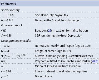
However, the second risk—low-frequency risk or rare event risk—remains problematic even for those investing for the long run. This risk refers to rare events that unpredictably lead to the sudden destruction of significant wealth.Footnote 1 The COVID-19 outbreak in the Spring of 2020 triggered the S&P 500 to suddenly lose approximately one-third of its value within just a few weeks. (Of course, within the same year, equity prices recovered rapidly alongside record earnings among technology companies, record low interest rates from rapid expansion in the money supply, and anticipation of a vaccine). But not all rare event shocks have been followed by rapid recovery. The S&P 500 reached a peak in October of 2007, lost more than half of its value in the Great Recession, and did not fully recover until more than 5 years had passed. This episode was problematic for workers on the verge of retirement who then faced the grim prospect of retiring with far less financial security than they had supposed. The same can be said of other rare events such as the dot.com recession in 2000 which featured a crash that erased almost half of the value of the S&P 500 and a slow recovery of asset prices lasting 7 years, as well as the Great Depression which quickly erased 86% of the value of the S&P 500 followed by a painfully slow recovery lasting 25 years.
Social Security was created in 1935 in response to the Great Depression with the goal to ensure the financial security of the elderly. The purpose of this paper is to examine the welfare role of Social Security as a safety net against rare event risk. To study this issue, we blend traditional Social Security welfare analysis—which compares ex ante lifetime utility with and without Social Security—with the dynamic stochastic control literature. We study a life-cycle model in which individuals make optimal consumption and saving decisions in the face of a large, negative shock to their private financial wealth occurring at an unknown time. Losing a large fraction of one’s financial wealth is relatively painless if the individual has not yet accumulated very much wealth, but such a shock can have a major impact on the individual’s standard of living if it occurs close to retirement when wealth is at a maximum. Not knowing when such a shock might occur complicates financial planning, and we consider a model in which Social Security is, essentially, a safe asset within the individual’s retirement portfolio.
In our baseline calibration, we consider the worst-known financial shock in modern history, the Great Depression. The shock wipes out 86% of the individual’s accumulated assets, matching the lost value in the S&P 500 from peak to trough, and this shock occurs at an unknown time. Both before and after the shock hits, we assume the individual’s assets grow at 8% per year to reflect long run real average equity returns in the USA. The individual has full information about the distribution of the rare event risk that they face, and they hedge this risk by optimizing their consumption and saving decisions as the solution to a dynamic stochastic life-cycle saving problem. In this setting (with full information and perfect optimization), we do not find a safety net rationale for Social Security. Instead, we find that Social Security reduces lifetime welfare by 7.64%.
However, perfect hedging and full information are strong assumptions that drive these negative results. Moving beyond our baseline analysis, we attempt to carefully study Social Security’s safety net role when there are limits to the individual’s optimization and information. We consider three extensions in which optimization or information are imperfect. First, since the dynamic hedging problem is hard to solve, we study the case in which the individual fails to hedge rare event risk but otherwise saves rationally in the sense of consumption smoothing over the life cycle. Second, we consider the case in which the individual behaves according to a sophisticated dynamic hedging problem but does so under a misspecification of risk. Misspecification seems particularly plausible given the difficulty with inferring the timing distribution of an event that is rarely observed. And third, we study the case in which a maximin policy maker bases their evaluation of Social Security on whether it improves individual welfare under the worst-case timing scenario of the shock hitting at the moment of retirement, which creates maximum destruction of wealth. In all of these cases, the welfare effect of Social Security can be far larger than in the baseline model, and in multiple cases, the effect is a large welfare gain rather than a welfare loss.
In sum, if individuals have full information about rare asset shocks and optimally hedge this risk by following the solution to a sophisticated model, then they do not need Social Security as a safety net. They do just fine on their own. However, if individuals fall short of optimal hedging or if there are limits to the information about rare event risk, there are plausible scenarios in which Social Security is quite valuable as a safety net.
Given Social Security’s status as the largest government program in operation, it’s not surprising that an enormous amount of literature considers its welfare role. One strand of this literature focuses on evaluating Social Security’s effectiveness as a solution to the problem of inadequate private saving for retirement.Footnote 2 Another strand focuses on Social Security’s role as a hedge against longevity risk.Footnote 3 And another strand considers its role in hedging lifetime earnings risk or reducing inequality.Footnote 4 Still other risks such as disability risk and survivor risk to the dependent spouse and children also have been thoroughly examined.Footnote 5 Interestingly, however, less work has been done to understand Social Security’s role in insuring individuals against rare event asset shocks, despite the fact that Social Security was created in response to the worst financial shock in modern American history. This paper contributes to the open question of how well Social Security protects people against such risks.
A few studies consider the role of Social Security when private asset returns are risky. For example, Feldstein and Ranguelova (Reference Feldstein and Ranguelova1998) assess the size of Social Security benefits relative to what could be financed privately with a portfolio of stocks and bonds whose annual returns are uncertain. Like our baseline model, they do not find much scope for Social Security as a safety net against risky financial markets. We add to their work by considering decision-making under uncertainty about the timing of rare event shocks like the Great Depression.
Peterman and Sommer (Reference Peterman and Sommer2019a) find that Social Security improved the welfare of most people who lived through the Great Depression, thereby explaining the program’s creation if not explaining its persistence. Interestingly, the welfare gains in their model are not because Social Security provided a safety net during a period of crises-indeed, the welfare gains would be even larger in their model had the program been implemented during a period of economic tranquility. Instead, the welfare gains to the initial generation are because they paid very little in taxes relative to the large, windfall benefits that they received. Also, the Great Depression shock takes agents in their setting by surprise, making their analysis a study of ex post welfare. We ask a different question. We consider ex ante welfare analysis. The main feature of our analysis is decision-making in the face of uncertainty about the timing of a large shock to asset values.Footnote 6
2. A model of optimal hedging under full information
2.1. Life-cycle consumption with rare event risk
Time is continuous and indexed by $t$
. An individual is born at
$t$
. An individual is born at $t=0$
, retires at date
$t=0$
, retires at date $t_R$
, and dies no later than
$t_R$
, and dies no later than $t=T$
. The probability of surviving to age
$t=T$
. The probability of surviving to age $t$
is
$t$
is $\Psi (t)$
. The individual receives income
$\Psi (t)$
. The individual receives income $y(t)$
over the life cycle which consists of after-tax labor income before retirement and Social Security benefits after retirement. Consumption is denoted
$y(t)$
over the life cycle which consists of after-tax labor income before retirement and Social Security benefits after retirement. Consumption is denoted $c(t)$
and saving is denoted
$c(t)$
and saving is denoted $k(t)$
. The interest rate is
$k(t)$
. The interest rate is $r$
; this is the rate of return at all times other than when the shock hits. The individual discounts future utility at the rate
$r$
; this is the rate of return at all times other than when the shock hits. The individual discounts future utility at the rate $\rho$
.
$\rho$
.
The instantaneous utility function is the CRRA function:
 \begin{equation} u(c)=\frac{c(t)^{1-\sigma }}{1-\sigma }. \end{equation}
The household faces a risk that they will experience a negative wealth shock at some point during their working life that makes the share $S$
of their assets disappear. The shock date
$S$
of their assets disappear. The shock date $t_1$
is a random variable with probability density
$t_1$
is a random variable with probability density $\phi (t_1)$
for
$\phi (t_1)$
for $t_1 \in [0,\infty ]$
. The one-time negative wealth shock reduces the household’s private savings by fraction
$t_1 \in [0,\infty ]$
. The one-time negative wealth shock reduces the household’s private savings by fraction $S$
. That is, the household only has
$S$
. That is, the household only has $(1-S)$
of their assets remaining after the shock. The household knows the size of
$(1-S)$
of their assets remaining after the shock. The household knows the size of $S$
, but does not know when
$S$
, but does not know when $S$
will occur.
$S$
will occur.
The rare event financial shock that we model has an asymmetric effect on positive and negative asset holdings. That is, we allow individuals to hold negative assets (debt), and in that case there is no change in the magnitude of their debt when a financial shock hits. The shock only reduces positive asset valuations.Footnote 7 Therefore, notationally, we denote the state dependency of the shock
 \begin{equation} S(k(t_{1}))=\boldsymbol{1}\{k(t_{1})\gt 0\}S, \end{equation}
where $\boldsymbol{1}\{k(t_{1})\gt 0\}$
is an indicator function that is equal to one when assets are positive and zero when assets are zero or negative.
$\boldsymbol{1}\{k(t_{1})\gt 0\}$
is an indicator function that is equal to one when assets are positive and zero when assets are zero or negative.
The household optimization problem is solved recursively, using the timing uncertainty methods from the stochastic control literature as in Cottle Hunt and Caliendo (Reference Cottle Hunt and Caliendo2021), Caliendo et al. (Reference Caliendo, Casanova, Gorry and Slavov2020), Caliendo et al. (Reference Caliendo, Gorry and Slavov2019), and Stokey (Reference Stokey2016).
2.1.1. Postshock problem
The negative wealth shock $S$
occurs at time
$S$
occurs at time $t_1\leq \infty$
. If the shock occurs before time
$t_1\leq \infty$
. If the shock occurs before time $T$
, the household solves the following deterministic, fixed-end point problem from the vantage point of the shock date:
$T$
, the household solves the following deterministic, fixed-end point problem from the vantage point of the shock date:
 \begin{equation} \max _{c(t)} \int _{t_1}^{T}e^{-\rho t}\Psi (t) u(c(t))dt, \end{equation}
subject to
 \begin{align} \dot{K}(t)=y(t)-c(t)+rK(t) \quad \textrm{for } t\in [t_1,T] \end{align}
 \begin{align} K(t_1)=k(t_1)(1-S(k(t_1))) \end{align}
 \begin{align} K(T)=0 \end{align}
 \begin{align} k(t_1) \textrm{ given, } S(k(t_1)) \textrm{ given, } t_1 \textrm{ given.} \end{align}
Here, $K(t)$
is the total financial wealth of the household after the shock takes place.
$K(t)$
is the total financial wealth of the household after the shock takes place. $K(t_1)$
is the share of private savings
$K(t_1)$
is the share of private savings $k(t_1)$
that remain immediately after the shock
$k(t_1)$
that remain immediately after the shock $S(k(t_1))$
occurs.
$S(k(t_1))$
occurs.
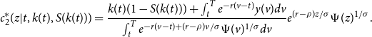
The solution to this problem is the consumption path $c^*_2(t|t_1,k(t_1),S(k(t_1)))$
which is the optimal path of consumption after the wealth shock has occurred. The subscript 2 indicates this is the path of post-shock consumption for
$c^*_2(t|t_1,k(t_1),S(k(t_1)))$
which is the optimal path of consumption after the wealth shock has occurred. The subscript 2 indicates this is the path of post-shock consumption for $ t\in [t_1,T]$
,
$ t\in [t_1,T]$
,
 \begin{equation} c^*_2(t|t_1,k(t_1),S(k(t_1))) = \frac{k(t_1)(1-S(k(t_1))) + \int _{t_1}^{T}e^{-r(v-t_1)}y(v)dv}{\int _{t_1}^{T}e^{-r(v-t_1)+(r-\rho )v/\sigma }\Psi (v)^{1/\sigma }dv}e^{(r-\rho )t/\sigma } \Psi (t)^{1/\sigma }. \end{equation}
Note changing variable notation for convenience, we replace $t$
with
$t$
with $z$
and
$z$
and $t_1$
with
$t_1$
with $t$
. Hence, consumption on
$t$
. Hence, consumption on $z\in [t,T]$
for shock date
$z\in [t,T]$
for shock date $t$
is
$t$
is
 \begin{equation} c^*_2(z|t,k(t),S(k(t))) = \frac{k(t)(1-S(k(t)))+ \int _{t}^{T}e^{-r(v-t)}y(v)dv}{\int _{t}^{T}e^{-r(v-t)+(r-\rho )v/\sigma }\Psi (v)^{1/\sigma }dv}e^{(r-\rho )z/\sigma } \Psi (z)^{1/\sigma }. \end{equation}
2.1.2. Preshock problem
Next we solve the dynamic stochastic problem of a household that hedges the timing risk of shock $S(k(t))$
, from the perspective of time 0.
$S(k(t))$
, from the perspective of time 0.
The household’s expected utility is
 \begin{equation} \begin{split} \mathbb{E}(U)& =\int _{0}^{T} \phi (t) \left (\int _{0}^{t}e^{-\rho z} \Psi (z)u(c(z))dz +\int _{t}^{T}e^{-\rho z} \Psi (z)u(c^*_2(z|t,k(t),S(k(t))))dz\right ) dt\\[5pt] &\!\quad+ \int _{T}^{\infty }\phi (t)\left (\int _{0}^{T}e^{-\rho z} \Psi (z)u(c(z))dz \right )dt, \end{split} \end{equation}
which can be rewritten more compactly using the properties of iterated integrals
 \begin{equation} \mathbb{E}(U) = \int _0^{T} \left [ \left (\int _t^{\infty }\phi (t_1)dt_1 \right ) e^{-\rho t}\Psi (t)u(c(t)) + \phi (t) U_2(t,k(t),S(k(t))) \right ] dt \end{equation}
where
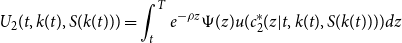 \begin{equation} U_2(t,k(t),S(k(t)))=\int _t^{T}e^{-\rho z}\Psi (z)u(c^*_2(z|t,k(t),S(k(t))))dz \end{equation}
and $c^*_2(z|t,k(t),S(k(t)))$
is given by (9).
$c^*_2(z|t,k(t),S(k(t)))$
is given by (9).
Thus, the preshock household’s stochastic optimization problem can be written neatly as a Pontryagin problem
 \begin{gather} \max _{c(t)_{t\in [0,T]}} \int _0^{T} \left [ \left (\int _t^{\infty }\phi (t_1)dt_1 \right ) e^{-\rho t}\Psi (t)u(c(t)) + \phi (t) U_2(t,k(t),S(k(t))) \right ] dt \end{gather}
subject to
 \begin{align} \dot{k}(t) = r k(t) + y(t) -c(t) \quad \textrm{for } t\in [0,T] \end{align}
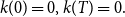 \begin{align} k(0)=0, k(T)=0. \end{align}
The Hamiltonian $\mathcal{H}$
with multiplier
$\mathcal{H}$
with multiplier $\lambda (t)$
for this problem is
$\lambda (t)$
for this problem is
 \begin{equation} \begin{split} \mathcal{H}= & \left (\int _t^{\infty }\phi (t_1)dt_1 \right ) e^{-\rho t}\Psi (t)u(c(t)) \\[5pt] &+ \phi (t) U_2(t,k(t),S(k(t))) +\lambda (t) \left ( r k(t) + y(t) -c(t) \right ). \end{split} \end{equation}
The necessary conditions are
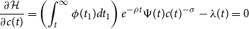 \begin{align} \frac{\partial \mathcal{H}}{\partial c(t)}=\left (\int _t^{\infty }\phi (t_1)dt_1 \right ) e^{-\rho t}\Psi (t) c(t)^{-\sigma }-\lambda (t)=0 \end{align}
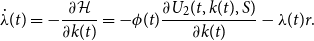 \begin{align} \dot{\lambda }(t) = -\frac{\partial \mathcal{H}}{\partial k(t)} = -\phi (t) \frac{\partial U_2(t,k(t),S)}{\partial k(t)} - \lambda (t)r. \end{align}
Note, substituting $c^*_2(z|t,k(t),S(k(t)))$
into
$c^*_2(z|t,k(t),S(k(t)))$
into $U_2(t,k(t),S(k(t)))$
the partial derivative
$U_2(t,k(t),S(k(t)))$
the partial derivative
 \begin{equation} \frac{\partial U_2(t,k(t),S(k(t)))}{\partial k(t)}=\left ( \frac{k(t)(1-S(k(t))) + \int _{t}^{T}e^{-r(v-t)}y(v)dv}{\int _{t}^{T}e^{-r(v-t)+(r-\rho )v/\sigma }\Psi (v)^{1/\sigma }dv}\right )^{-\sigma }(1-S(k(t)))e^{-rt}. \end{equation}
Insert (19) and (17) into (18)
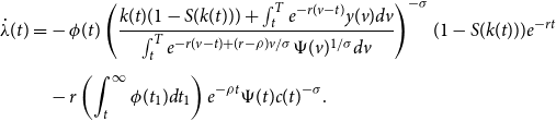 \begin{equation} \begin{split} \dot{\lambda }(t)=&-\phi (t) \left ( \frac{k(t)(1-S(k(t))) + \int _{t}^{T}e^{-r(v-t)}y(v)dv}{\int _{t}^{T}e^{-r(v-t)+(r-\rho )v/\sigma }\Psi (v)^{1/\sigma }dv}\right )^{-\sigma }(1-S(k(t)))e^{-rt} \\[5pt] &-r\left (\int _t^{\infty }\phi (t_1)dt_1 \right ) e^{-\rho t} \Psi (t)c(t)^{-\sigma }. \end{split} \end{equation}
Differentiate (17) with respect to $t$
$t$
 \begin{equation} \begin{split} 0=&-\phi (t)e^{-\rho t}\Psi (t)c(t)^{-\sigma }+\left (\int _t^{\infty }\phi (t_1)dt_1 \right ) \left (\dot{\Psi }(t)e^{-\rho t}-\rho \Psi (t)e^{-\rho t} \right )c(t)^{-\sigma }\\[5pt] &-\left (\int _t^{\infty }\phi (t_1)dt_1 \right ) \sigma e^{-\rho t}\Psi (t)c(t)^{-\sigma -1}\dot{c}(t)-\dot{\lambda }(t). \end{split} \end{equation}
Combine (20) and (21) to obtain the Euler equation in closed form
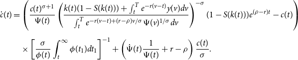 \begin{equation} \begin{split} \dot{c}(t) &=\left ( \frac{c(t)^{\sigma +1}}{\Psi (t)} \left ( \frac{k(t)(1-S(k(t))) + \int _{t}^{T}e^{-r(v-t)}y(v)dv}{\int _{t}^{T}e^{-r(v-t)+(r-\rho )v/\sigma }\Psi (v)^{1/\sigma }dv}\right )^{-\sigma }(1-S(k(t)))e^{(\rho -r)t}-c(t)\right )\\[5pt] & \quad\times \left [\frac{\sigma }{\phi (t)}\int _t^{\infty }\phi (t_1)dt_1\right ]^{-1} + \left (\dot{\Psi }(t)\frac{1}{\Psi (t)} +r-\rho \right )\frac{c(t)}{\sigma }. \end{split} \end{equation}
The optimal path of consumption and assets prior to the shock $(c^*_1(t),k^*_1(t))_{t\in [0,T]}$
obey the Euler equation and the constraints.
$(c^*_1(t),k^*_1(t))_{t\in [0,T]}$
obey the Euler equation and the constraints.
2.2. Computational method
Although our model is solved analytically for both the preshock and postshock timepaths of consumption and savings, we must employ a recursive computational method to identify the initial consumption level. We utilize our analytical solutions to identify initial consumption as follows:
Step 1. Compute $c_{2}^{\ast }(z|t,k(t),S(k(t)))$
for given shock date
$c_{2}^{\ast }(z|t,k(t),S(k(t)))$
for given shock date $t$
, given asset holdings at that date
$t$
, given asset holdings at that date $k(t)$
, and given shock size
$k(t)$
, and given shock size $S(k(t))$
.
$S(k(t))$
.
Step 2. Guess $c(0)$
.
$c(0)$
.
Step 3. Given the guessed value of $c(0)$
together with
$c(0)$
together with $k(0)=0$
, use the Euler equation
$k(0)=0$
, use the Euler equation $\dot{c}(t)$
and law of motion for capital
$\dot{c}(t)$
and law of motion for capital $\dot{k}(t)$
, which themselves depend on the post-shock consumption path
$\dot{k}(t)$
, which themselves depend on the post-shock consumption path $c_{2}^{\ast }(z|t,k(t),S(k(t)))$
, to shoot forward in time to construct the pre-shock timepaths
$c_{2}^{\ast }(z|t,k(t),S(k(t)))$
, to shoot forward in time to construct the pre-shock timepaths $c(t)$
and
$c(t)$
and $k(t)$
.
$k(t)$
.
Step 4. Check the terminal value of pre-shock capital to see if $k(T)=0$
. If yes, then we have found our solution pre-shock consumption and saving paths
$k(T)=0$
. If yes, then we have found our solution pre-shock consumption and saving paths $c_{1}^{\ast }(t)$
and
$c_{1}^{\ast }(t)$
and $k_{1}^{\ast }(t)$
. If not, go back to step 2 and repeat.
$k_{1}^{\ast }(t)$
. If not, go back to step 2 and repeat.
2.3. Calibration
Our baseline calibration strategy is to maximize the potential safety net feature of Social Security by assuming that a modern individual faces risk of a financial shock that is proportional to the stock market crash of the Great Depression. This means that we will calibrate things like income, career length, longevity, and Social Security to modern specifications, and we will assume the individual faces financial risk like that experienced by past generations who endured the Great Depression.Footnote 8
We assume the individual enters the model at age 18 ( $t=0$
), retires at age 67 (
$t=0$
), retires at age 67 ( $t_R=49$
), and lives to a maximum age of 100 (
$t_R=49$
), and lives to a maximum age of 100 ( $T=82$
). We calibrate the survival function and wage income following Cottle Hunt and Caliendo (Reference Cottle Hunt and Caliendo2021). We calibrate the survival function as
$T=82$
). We calibrate the survival function and wage income following Cottle Hunt and Caliendo (Reference Cottle Hunt and Caliendo2021). We calibrate the survival function as
 \begin{equation} \Psi (t) = 1-(t/T)^{2.58} \end{equation}
to ensure that the ratio of workers to retirees is 3.3, which is approximately the average value in the USA during the period 2000–2010.Footnote
9
The life expectancy at $t=0$
implied by this survival function is age 77.1, which corresponds closely to the life expectancy from birth for the USA reported by the World Bank of 78.5 years. We parameterize
$t=0$
implied by this survival function is age 77.1, which corresponds closely to the life expectancy from birth for the USA reported by the World Bank of 78.5 years. We parameterize $y(t)$
to represent after-tax income before retirement and Social Security benefits after retirement. We use a 5th order polynomial to fit life-cycle wages to the data in Gourinchas and Parker (Reference Gourinchas and Parker2002)
$y(t)$
to represent after-tax income before retirement and Social Security benefits after retirement. We use a 5th order polynomial to fit life-cycle wages to the data in Gourinchas and Parker (Reference Gourinchas and Parker2002)
 \begin{equation} w(t)=\alpha (1+0.0244t-0.0001t^{2}+4(10)^{-5}t^{3}-2(10)^{-6}t^{4}+2(10)^{-8}t^{5}) \end{equation}
where $\alpha$
is chosen such that the average wage is equal to one.
$\alpha$
is chosen such that the average wage is equal to one.
We set the Social Security tax rate to $\tau =0.106$
, which corresponds to the employer and employee Old Age Survivors portion of Social Security. We assume the Social Security system has a balanced PAYGO budget, hence
$\tau =0.106$
, which corresponds to the employer and employee Old Age Survivors portion of Social Security. We assume the Social Security system has a balanced PAYGO budget, hence
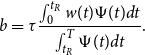 \begin{equation*} b=\tau \frac {\int _{0}^{t_{R}}w(t)\Psi (t)dt}{\int _{t_{R}}^{T}\Psi (t)dt}. \end{equation*}
Thus, $y(t)$
is given by
$y(t)$
is given by
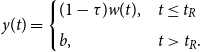 \begin{equation} y(t) = \begin{cases} (1-\tau )w(t), & t \leq t_R\\[5pt] b, & t\gt t_R. \end{cases} \end{equation}
We set the interest rate $r=0.08$
which corresponds to the average long-term real return on equities. We set
$r=0.08$
which corresponds to the average long-term real return on equities. We set $\sigma =3$
, which is a mid-point of the standard values used in the literature. Finally, we set the discount rate
$\sigma =3$
, which is a mid-point of the standard values used in the literature. Finally, we set the discount rate $\rho =0$
.
$\rho =0$
.
As our baseline parameterization for the rare event shock, we assume the risk of experiencing the shock is uniform and that the individual cannot escape the shock—it is sure to hit during their life cycle. Hence
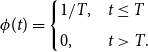 \begin{equation} \phi (t)=\begin{cases} 1/T, & t\leq T\\[5pt] 0, & t\gt T. \end{cases} \end{equation}
As a robustness check later in the paper, we explore a distribution that has positive mass beyond the maximum age $T$
. We calibrate the size of the shock
$T$
. We calibrate the size of the shock $S$
to correspond to the Great Depression. The S&P lost 86% of its value during the Great Depression, and so we set
$S$
to correspond to the Great Depression. The S&P lost 86% of its value during the Great Depression, and so we set $S=0.86$
.Footnote 10 Our baseline parameters are summarized in Table 1.
$S=0.86$
.Footnote 10 Our baseline parameters are summarized in Table 1.
Table 1. Summary of baseline calibration of parameters
2.4. Welfare
Our goal is to assess Social Security’s role as a safety net against rare event financial shocks to wealth. Our stylized model leaves out a number of Social Security’s features like disability insurance, spousal benefits, survivor insurance, and a benefit-earning rule that redistributes wealth from the rich to the poor. While these are important features, we view the simplicity of our baseline analysis as an advantage because it allows us to focus cleanly on the safety net rationale, which is our purpose. As a result, we are not in a position to make statements about Social Security’s overall welfare effects. Instead, we are drawing conclusions about a single mechanism in particular.
We measure the welfare effect of Social Security as the percentage of lifetime consumption the individual would be willing to give up to live in a world with Social Security relative to a Laissez Faire world with no Social Security.
Notationally, let $\mathbb{E}(U_{SS}^{\ast })$
stand for expected utility in a world with Social Security and following optimal consumption rules under uncertainty. Likewise let
$\mathbb{E}(U_{SS}^{\ast })$
stand for expected utility in a world with Social Security and following optimal consumption rules under uncertainty. Likewise let $\mathbb{E}(U_{LF}^{\ast })$
stand for expected utility in a Laissez Faire world without Social Security and following optimal consumption rules in that environment. With CRRA utility, the fraction of lifetime consumption the individual would give up to participate in Social Security is
$\mathbb{E}(U_{LF}^{\ast })$
stand for expected utility in a Laissez Faire world without Social Security and following optimal consumption rules in that environment. With CRRA utility, the fraction of lifetime consumption the individual would give up to participate in Social Security is
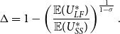 \begin{equation} \Delta =1-\left ( \frac{\mathbb{E}(U_{LF}^{\ast })}{\mathbb{E}(U_{SS}^{\ast })}\right ) ^{\frac{1}{1-\sigma }}. \end{equation}
We calibrate the size of the shock to correspond to the Great Depression: $S=0.86$
. Even in this extreme case, we find the welfare effect of Social Security to be negative,
$S=0.86$
. Even in this extreme case, we find the welfare effect of Social Security to be negative, $\Delta =-7.64\%$
. That is, an individual would be need to receive an additional 7.64% of lifetime consumption in order to compensate for participating in Social Security.
$\Delta =-7.64\%$
. That is, an individual would be need to receive an additional 7.64% of lifetime consumption in order to compensate for participating in Social Security.
What is the intuition for this result? The basic answer is that US equities are still a very good deal, even when individuals face catastrophic, rare event risk. An 8% return compounded annually, together with the risk of a one-time shock equivalent to the Great Depression (86% instantaneous loss in wealth), still compares favorably to the implicit rate of return in a Pay-As-You-Go Social Security program. And this is true even after accounting for the life annuity feature of Social Security.
The intuition is also visible in the possible timepaths of consumption over the life cycle with and without Social Security. Figure 1 plots a few possible paths of realized life cycle consumption with and without Social Security, given different possible dates for the shock (specifically ages 38, 48, 58, 68 and 78). The solid green line plots the Laissez Faire con- sumption paths and the dashed blue lines are with Social Security. Consumption is generally higher without Social Security.
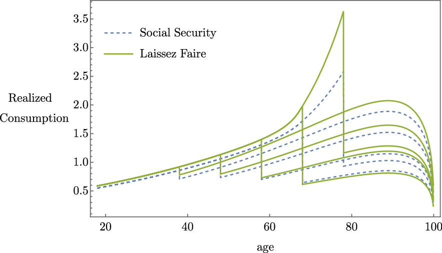
Figure 1. Realized consumption given $S=0.86$
, with and without Social Security.
$S=0.86$
, with and without Social Security.
This negative welfare result is important because in some ways we have stacked our analysis in favor of Social Security in our choice of modeling assumptions. We assume the financial shock is guaranteed to happen; we assume the shock will be the biggest possible shock in modern history; and, we assume the individual’s only choice for private saving is a risky asset. By assuming the individual faces an inescapable, large shock with no access to a safe asset, the individual is left completely exposed to risk and Social Security’s safety net role should be maximized. And yet we do not find a safety net role for Social Security.
However, we will show in Section 3 that our baseline assumptions about optimal hedging under full information are driving the negative welfare result. Relaxing these assumptions will create space for large welfare gains.
2.5. Decomposition
We decompose the welfare effect of Social Security into the portion that comes from the provision of longevity insurance and the portion that comes from the provision of a financial safety net. To do this, we turn off financial risk by setting the asset shock to $S=0$
and we find that
$S=0$
and we find that $\Delta =-10.91\%$
. Consumption with and without Social Security when
$\Delta =-10.91\%$
. Consumption with and without Social Security when $S=0$
is depicted in Figure 2. Since the shock is set to zero, there is only one realized consumption path and consumption is everywhere higher without Social Security. This welfare effect is worse (more negative) than the combined welfare effect of insurance against both longevity and asset risk which was −7.64% in our baseline model. This suggests that Social Security is less harmful in the presence of rare event risk.
$S=0$
is depicted in Figure 2. Since the shock is set to zero, there is only one realized consumption path and consumption is everywhere higher without Social Security. This welfare effect is worse (more negative) than the combined welfare effect of insurance against both longevity and asset risk which was −7.64% in our baseline model. This suggests that Social Security is less harmful in the presence of rare event risk.
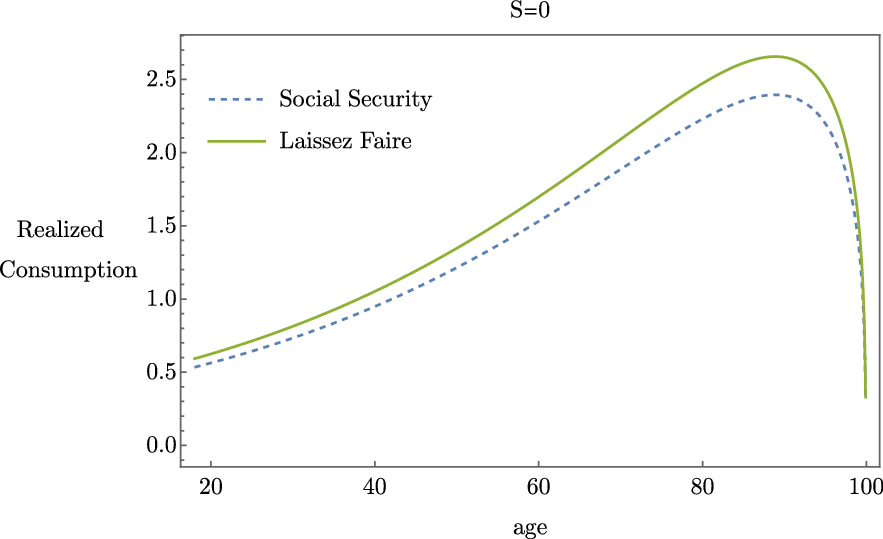
Figure 2. Realized consumption given $S=0$
, with and without Social Security.
$S=0$
, with and without Social Security.
As an alternative decomposition, we turnoff both the asset risk and the asset reward by setting $S=0$
and
$S=0$
and $r=0$
. We find that
$r=0$
. We find that $\Delta =11.57\%$
in this case. This large positive welfare effect is due to the well-known annuitization feature of Social Security. An individual would rather pay Social Security taxes and receive a Social Security annuity during retirement rather than invest in a riskless asset with zero return. Consumption with and without Social Security when
$\Delta =11.57\%$
in this case. This large positive welfare effect is due to the well-known annuitization feature of Social Security. An individual would rather pay Social Security taxes and receive a Social Security annuity during retirement rather than invest in a riskless asset with zero return. Consumption with and without Social Security when $S=0$
and
$S=0$
and $r=0$
is depicted in Figure 3. In this case, consumption is everywhere higher with Social Security.
$r=0$
is depicted in Figure 3. In this case, consumption is everywhere higher with Social Security.
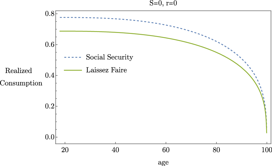
Figure 3. Realized consumption given $S=0$
and
$S=0$
and $r=0$
, with and without Social Security.
$r=0$
, with and without Social Security.
2.6. Robustness checks
Some of the parameters that we use in our baseline analysis are unobservable and could have direct bearing on our welfare calculations. In this section, we briefly discuss these issues before addressing more fundamental extensions.
Our baseline value of 3 for the coefficient of relative risk aversion ( $\sigma$
) falls within a standard range of values used in the life-cycle consumption literature, though values as low as 0.5 and as high as 5 are also used. The welfare effect of Social Security is −8.64% and −7.08% with these values, compared to our baseline value −7.64%. Hence, while different levels of risk aversion change the specific welfare effect of Social Security, our overall conclusion about its role as a safety net is unchanged.
$\sigma$
) falls within a standard range of values used in the life-cycle consumption literature, though values as low as 0.5 and as high as 5 are also used. The welfare effect of Social Security is −8.64% and −7.08% with these values, compared to our baseline value −7.64%. Hence, while different levels of risk aversion change the specific welfare effect of Social Security, our overall conclusion about its role as a safety net is unchanged.
Similarly, our use of a 0% discount rate is not uncommon, but it is also common to see values as high as 5% used in the life-cycle literature. The welfare effect of Social Security is −7.89% under this assumption. Again, no material change to our conclusions thus far.
We assumed the financial shock was distributed uniformly over the life cycle of the individual. This is a reasonable starting assumption and it helps to stack the analysis in favor of Social Security: if the individual cannot escape experiencing the shock at some point (because the upper support of the shock coincides with the maximum age of the individual), then Social Security would be more attractive as a safety net than if there was a chance the individual may never experience the negative shock. However, our uniform assumption has a subtle side effect: if the shock has not yet happened, then as the individual ages they become increasingly sure that it will happen to them. Indeed, as the individual approaches the maximum model age, the probability that the shock strikes will spike to 100% conditional on it not happening yet. This is a mathematical definition of any truncated distribution, and yet there is no reason that a rare financial shock would increase in relative likelihood as an individual ages.
As an alternative, we consider the exponential density
 \begin{equation} \phi (t)=\gamma e^{-\gamma t}\textrm{, for }t\in \lbrack 0,\infty ]\textrm{ and }\gamma \gt 0. \end{equation}
This density is memoryless: if the shock has not occurred by date $x$
, the likelihood of the shock occurring between
$x$
, the likelihood of the shock occurring between $x$
and
$x$
and $x+\delta$
does not depend on
$x+\delta$
does not depend on $x$
. As an example, we calibrate
$x$
. As an example, we calibrate $\gamma$
by assuming there is a 50% chance that a financial crash like the Great Depression does not happen within the individual’s maximum lifespan; hence,
$\gamma$
by assuming there is a 50% chance that a financial crash like the Great Depression does not happen within the individual’s maximum lifespan; hence, $\gamma =-\ln (0.5)/82$
. The welfare effect of Social Security is −7.42% under this assumption. Note that while the need for a safety net is intuitively weakened if there is a chance that such a net is never needed, the exponential distribution considered here also rearranges the shock probabilities over the lifespan of the individual, with the most weight during the earliest years of life. This secondary effect virtually washes out the first effect and leaves the overall welfare effect of Social Security quite similar to our baseline estimate.
$\gamma =-\ln (0.5)/82$
. The welfare effect of Social Security is −7.42% under this assumption. Note that while the need for a safety net is intuitively weakened if there is a chance that such a net is never needed, the exponential distribution considered here also rearranges the shock probabilities over the lifespan of the individual, with the most weight during the earliest years of life. This secondary effect virtually washes out the first effect and leaves the overall welfare effect of Social Security quite similar to our baseline estimate.
Lastly, we assumed a real interest rate of $r=0.08$
which corresponds to the average annual real return on equities in the USA over the last 50–100 years. The welfare effect of Social Security is decreasing in the interest rate. That is, Social Security reduces welfare less (or increases welfare more) if the interest rate is lower. Holding the other parameters fixed at their baseline values, the welfare effect of Social Security is −2.47% for an interest rate of
$r=0.08$
which corresponds to the average annual real return on equities in the USA over the last 50–100 years. The welfare effect of Social Security is decreasing in the interest rate. That is, Social Security reduces welfare less (or increases welfare more) if the interest rate is lower. Holding the other parameters fixed at their baseline values, the welfare effect of Social Security is −2.47% for an interest rate of $r=0.06$
, zero for
$r=0.06$
, zero for $r=0.054$
, 1.82% for
$r=0.054$
, 1.82% for $r=0.05$
, and 7.9% for
$r=0.05$
, and 7.9% for $r=0.04$
.
$r=0.04$
.
3. Departures from optimal hedging under full information
There may be limits on the degree to which people are able to hedge rare event risk in actuality. In the analysis above, the individual has perfect information about the distribution of timing risk, and then is able to solve a complex dynamic stochastic hedging problem to protect themselves against this risk. To study the importance of these strong assumptions, in this section, we consider three possibilities.
First, we assume the individual does not hedge the risk at all but otherwise behaves optimally in saving for retirement in the face of survival uncertainty. The policy maker is aware of the true distribution of rare event risk and evaluates the performance of Social Security through the lens of whether it improves the ex ante expected utility of the individual. We find that the large welfare losses from Social Security in the baseline analysis with optimal hedging now become large welfare gains when the individual fails to hedge.
Second, we consider the case in which the true distribution of risk is unknown to the individual. Consequently, the individual solves the dynamic stochastic hedging problem featured in the baseline analysis above, but they do so under a misspecification of rare event risk. We find that the direction of the misspecification is important: relative to the baseline model with correct risk specification, Social Security is less negative for individuals who underestimate the risk they face. However, Social Security is even more harmful for individuals who overestimate the risk they face.
Third, we study the case in which the policy maker evaluates Social Security based on its performance under the worst possible shock timing, which is the date of retirement when the individual’s wealth is at a maximum. We find this dampens the welfare losses associated with Social Security in our baseline parameterization and leads to welfare gains if the risk is distributed exponentially. In other words, simply switching the policy maker’s welfare criteria from expected utility to maximin can be enough to justify Social Security as a safety net against rare event risk.
3.1. Failing to hedge
Up to this point in the paper, we have assumed the individual has full information about the risks that they face and that they behave optimally in the face of this risk. In this case, we found above that Social Security is unable to confer any welfare gains (as a safety net against rare event risk), at least at the parameterizations that we have highlighted. Our baseline model highlights that an individual who saves optimally in the face of this risk does not need a Social Security program to help manage this risk.
In this section, we consider an alternative model. In actuality, for a variety of reasons, individuals may not solve a sophisticated dynamic hedging problem. For instance, individuals may lack information on the nature of rare event risk, and without any information on the distribution of the risk, they may choose to ignore it and instead base their financial plans on expected (average) returns. Similarly, in financial planning, people often say things like, “when saving over long time horizons, equities pay better than bonds on average” and then use this fact as a justification for basing financial projections on a rate of return to saving that equals the average long-run return to equities, without explicitly modeling rare event risk. Moreover, the complexity of optimal hedging may limit its attractiveness as a saving plan, with individuals instead opting for simple rules. Whatever the cause for failing to hedge, in this section we study the welfare effect of Social Security when rare event risk exists but is not incorporated into the household’s saving plan. Unlike the previous section which struggles to find a rationale for Social Security as a safety net, in this section, the welfare gains of Social Security are large.
We consider a household that plans consumption and saving to maximize lifetime utility, ignoring the possibility of rare event risk. The household solves the following deterministic problem:
 \begin{equation} \max _{c(t)} \int _{0}^{T}e^{-\rho t}\Psi (t) u(c(t))dt, \end{equation}
subject to
 \begin{align} \dot{k}(t)=y(t)-c(t)+rk(t) \quad \textrm{for } t\in [0,T] \end{align}
 \begin{align} k(0)=0, k(T)=0. \end{align}
The solution to this problem is the planned consumption path
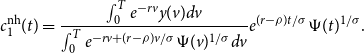 \begin{equation} c^{\textrm{nh}}_1(t) = \frac{ \int _{0}^{T}e^{-rv}y(v)dv}{\int _{0}^{T}e^{-rv+(r-\rho )v/\sigma }\Psi (v)^{1/\sigma }dv}e^{(r-\rho )t/\sigma } \Psi (t)^{1/\sigma }. \end{equation}
The superscript $\textrm{nh}$
on
$\textrm{nh}$
on $c^{\textrm{nh}}_1(t)$
indicates this is planned consumption with no hedging. The subscript on
$c^{\textrm{nh}}_1(t)$
indicates this is planned consumption with no hedging. The subscript on $c^{\textrm{nh}}_1(t)$
indicates that this is the consumption path the household follows until the rare event shock occurs (if it occurs at all).
$c^{\textrm{nh}}_1(t)$
indicates that this is the consumption path the household follows until the rare event shock occurs (if it occurs at all).
If the rare event shock occurs during the household’s lifetime (at date $t$
), we assume the household reoptimizes and follows the postshock consumption path
$t$
), we assume the household reoptimizes and follows the postshock consumption path $c^*_2(z|t,k(t),S(k(t)))$
for
$c^*_2(z|t,k(t),S(k(t)))$
for $z \in [t,T]$
, as given in equation (9). The consumption path
$z \in [t,T]$
, as given in equation (9). The consumption path $c^*_2(z|t,k(t),S(k(t)))$
is optimal conditional on shock date
$c^*_2(z|t,k(t),S(k(t)))$
is optimal conditional on shock date $t$
, assets
$t$
, assets $k(t)$
, and shock
$k(t)$
, and shock $S(k(t))$
. The assets the household owns at the time of the shock are determined by the law of motion equation (30) and the planned consumption path
$S(k(t))$
. The assets the household owns at the time of the shock are determined by the law of motion equation (30) and the planned consumption path $c^{\textrm{nh}}_1(t)$
.
$c^{\textrm{nh}}_1(t)$
.
Since this household does not hedge the rare event risk, they are surprised if the shock occurs in their lifetime. The realized life-cycle consumption path of the household given shock date $t$
is
$t$
is $c^{\textrm{nh}}_1(z)$
prior to the shock for
$c^{\textrm{nh}}_1(z)$
prior to the shock for $z\lt t$
, and
$z\lt t$
, and $c^*_2(z|t,k(t),S(k(t)))$
for
$c^*_2(z|t,k(t),S(k(t)))$
for $t\leq z\leq T$
following the shock.
$t\leq z\leq T$
following the shock.
We measure the welfare effect of Social Security from the perspective of a social planner who knows that the household does not hedge against the rare event risk. The social planner knows that the household will follow consumption path $c^{\textrm{nh}}_1(z)$
prior to the shock and the consumption path
$c^{\textrm{nh}}_1(z)$
prior to the shock and the consumption path $c^*_2(z|t,k(t),S(k(t)))$
after the shock. The planner calculates ex ante expected utility by computing the life-cycle utility for the realized path of consumption the household would experience for every possible shock date and weighing each path by how likely the shock is to occur at that date. Ex ante expected utility is given by
$c^*_2(z|t,k(t),S(k(t)))$
after the shock. The planner calculates ex ante expected utility by computing the life-cycle utility for the realized path of consumption the household would experience for every possible shock date and weighing each path by how likely the shock is to occur at that date. Ex ante expected utility is given by
 \begin{equation} \mathbb{E}(U^{\textrm{nh}}) = \int _0^{T} \left [ \left (\int _t^{\infty }\phi (t_1)dt_1 \right ) e^{-\rho t}\Psi (t)u(c^{\textrm{nh}}_1(t)) + \phi (t) U_2(t,k(t),S(k(t))) \right ] dt \end{equation}
where
 \begin{equation} U_2(t,k(t),S(k(t)))=\int _t^{T}e^{-\rho z}\Psi (z)u(c^*_2(z|t,k(t),S(k(t))))dz \end{equation}
and $c^*_2(z|t,k(t),S(k(t)))$
is given by (9).
$c^*_2(z|t,k(t),S(k(t)))$
is given by (9).
Notationally, let $\mathbb{E}(U_{\textrm{SS}}^{\textrm{nh}})$
stand for expected utility in a world with Social Security and no hedging. Likewise let
$\mathbb{E}(U_{\textrm{SS}}^{\textrm{nh}})$
stand for expected utility in a world with Social Security and no hedging. Likewise let $\mathbb{E}(U_{\textrm{LF}}^{\textrm{nh}})$
stand for expected utility in a Laissez Faire world without Social Security and no hedging. With CRRA utility, the consumption equivalent variation is
$\mathbb{E}(U_{\textrm{LF}}^{\textrm{nh}})$
stand for expected utility in a Laissez Faire world without Social Security and no hedging. With CRRA utility, the consumption equivalent variation is
 \begin{equation} \Delta ^{\textrm{nh}} =1-\left ( \frac{\mathbb{E}(U_{\textrm{LF}}^{\textrm{nh}})}{\mathbb{E}(U_{\textrm{SS}}^{\textrm{nh}})}\right ) ^{\frac{1}{1-\sigma }}. \end{equation}
The consumption equivalent variation is the percentage of lifetime consumption the individual who does not hedge rare event risk would be willing to give up to live in a world with Social Security relative to a Laissez Faire world with no Social Security. Note that our welfare comparison takes into consideration the distribution of rare event risk, even though the household itself does not incorporate this information into their consumption and saving plan. As in the previous section, a positive number indicates that Social Security makes the individual better off.
Using our baseline parameters, we find $\Delta ^{\textrm{nh}}=16.39\%$
. That is, a household who does not hedge rare event risk is made better off by participating in Social Security by an amount equivalent to about 16% of lifetime consumption. This large positive welfare effect stands in stark contrast to the negative welfare effect we found for households who optimally hedge rare event risk. Social Security is able to confer large welfare gains to households who do not hedge rare event risk by crowding out the risky assets the household owns and offering a safe asset (albeit, an asset with a low rate of return.). Households who do not hedge their rare event risk are made much better off in this scenario.
$\Delta ^{\textrm{nh}}=16.39\%$
. That is, a household who does not hedge rare event risk is made better off by participating in Social Security by an amount equivalent to about 16% of lifetime consumption. This large positive welfare effect stands in stark contrast to the negative welfare effect we found for households who optimally hedge rare event risk. Social Security is able to confer large welfare gains to households who do not hedge rare event risk by crowding out the risky assets the household owns and offering a safe asset (albeit, an asset with a low rate of return.). Households who do not hedge their rare event risk are made much better off in this scenario.
The positive welfare effect of Social Security is robust across several different parameter combinations, including when the shock distribution is calibrated to be an exponential distribution as in equation (28), in which case $\Delta ^{\textrm{nh}}=6.38\%$
.
$\Delta ^{\textrm{nh}}=6.38\%$
.
We also conduct an alternative welfare comparison to see how much better off the household who does not hedge rare event risk would be if they were able to optimally hedge. Specifically, we compute the percentage of lifetime consumption the individual who does not hedge rare event risk would be willing to give up to optimally hedge rare event risk:
 \begin{equation} \Gamma =1-\left ( \frac{\mathbb{E}(U_{\textrm{LF}}^{\textrm{nh}})}{\mathbb{E}(U_{\textrm{LF}}^{*})}\right ) ^{\frac{1}{1-\sigma }}. \end{equation}
Here, $\mathbb{E}(U_{\textrm{LF}}^{\textrm{nh}})$
stands for expected utility following the no-hedging consumption path
$\mathbb{E}(U_{\textrm{LF}}^{\textrm{nh}})$
stands for expected utility following the no-hedging consumption path $c^{\textrm{nh}}_1(z)$
prior to the shock and the consumption path
$c^{\textrm{nh}}_1(z)$
prior to the shock and the consumption path $c^*_2(z|t,k(t),S(k(t)))$
following the shock in the Laissez Faire economy. Similarly,
$c^*_2(z|t,k(t),S(k(t)))$
following the shock in the Laissez Faire economy. Similarly, $\mathbb{E}(U_{\textrm{LF}}^{*})$
indicates expected lifetime utility with optimal hedging.
$\mathbb{E}(U_{\textrm{LF}}^{*})$
indicates expected lifetime utility with optimal hedging.
This comparison allows us to see how much a household is harmed by not hedging rare event risk. Using our baseline parameters, we find the welfare gain of optimal hedging $\Gamma =27.44\%$
. The welfare gain of optimal hedging in Laissez Faire essentially shows the size of the problem of ignoring rare event risk. Participating in Social Security is not as good as optimally hedging, but does a reasonably good job helping households hedge rare event risk (by providing a safe asset). Recall, the welfare gain of Social Security is 16.39% for households that do not hedge rare event risk. Hence, the welfare gain of Social Security is about 60% of the welfare gain of optimally hedging, for households that ignore rare event risk.
$\Gamma =27.44\%$
. The welfare gain of optimal hedging in Laissez Faire essentially shows the size of the problem of ignoring rare event risk. Participating in Social Security is not as good as optimally hedging, but does a reasonably good job helping households hedge rare event risk (by providing a safe asset). Recall, the welfare gain of Social Security is 16.39% for households that do not hedge rare event risk. Hence, the welfare gain of Social Security is about 60% of the welfare gain of optimally hedging, for households that ignore rare event risk.
Using the exponential shock distribution as in (28), we find the welfare gain of optimal hedging $\Gamma =14.14\%$
in Laissez Faire. With this parameterization, Social Security is able to generate about 45% of the welfare gain of optimally hedging rare event risk.
$\Gamma =14.14\%$
in Laissez Faire. With this parameterization, Social Security is able to generate about 45% of the welfare gain of optimally hedging rare event risk.
3.2. Misspecification of risk
Rare event shocks are, by definition, seldom observed in reality. Therefore, it may be difficult for decision makers to know the distribution of the risk. To infer the distribution, one would need to observe many historical instances. Such inference is possible with high frequency, stationary risk but not with truly rare events.
To further connect our model to reality, in this section, we explore the possibility that the true distribution of timing risk is unknown to the individual decision maker. Instead, the individual makes decisions to hedge risk that are based upon an incorrect distribution of the risk. This exercise tells us how the welfare gains from Social Security are affected by risk misspecification, which seems especially relevant given the difficulty of drawing accurate inferences about the distribution of rare event risk.
We assume the risk of the rare event is distributed exponentially as in equation (28)
 \begin{equation*} \phi (t)=\gamma e^{-\gamma t}\text {, for }t\in \lbrack 0,\infty ]\text { and }\gamma \gt 0. \end{equation*}
Suppose the true distribution has a parameter $\gamma =-\ln (0.5)/82$
which corresponds to a 50% chance of the shock occurring within the individual’s maximum lifespan. However, the individual decision-maker does not know
$\gamma =-\ln (0.5)/82$
which corresponds to a 50% chance of the shock occurring within the individual’s maximum lifespan. However, the individual decision-maker does not know $\gamma$
and assumes the shock is instead distributed
$\gamma$
and assumes the shock is instead distributed
 \begin{equation} \phi (t)=\omega e^{-\omega t}\textrm{, for }t\in \lbrack 0,\infty \rbrack, \end{equation}
where $\omega$
is a multiple of
$\omega$
is a multiple of $\gamma$
. We consider four cases:
$\gamma$
. We consider four cases: $\omega =4\gamma$
,
$\omega =4\gamma$
, $\omega =2\gamma$
,
$\omega =2\gamma$
, $\omega =1/2\gamma$
, and
$\omega =1/2\gamma$
, and $\omega =1/4\gamma$
, which correspond to the individual believing the shock will occur within the maximum lifespan with probability 0.94, 0.75, 0.29, and 0.16, respectively.
$\omega =1/4\gamma$
, which correspond to the individual believing the shock will occur within the maximum lifespan with probability 0.94, 0.75, 0.29, and 0.16, respectively.
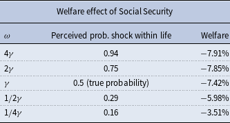
We solve for the individual’s optimal consumption-saving rule just like in Section 2, but now we assume the individual applies the wrong distribution of risk [equation (37)] and therefore optimizes the wrong expected utility function. Hence, the individual is sophisticated in their optimization behavior but they lack knowledge of the true distribution of risk. Then, in the welfare analysis, we apply the true distribution of risk [equation (28)] in our assessment of the welfare effect of Social Security.
Our results are presented in Table 2. We find that the welfare effect of Social Security is decreasing in the perceived likelihood of the rare event shock occurring. That is, individuals who believe the shock is more likely to occur than the true distribution are harmed more by Social Security than if they knew the risk. Similarly, individuals who do not believe the shock is as likely to occur are less harmed by Social Security. This is because Social Security is more helpful (less negative welfare effect) for households who are not as prepared for a rare event to strike. And for those who overestimate the risk they face—and therefore “over hedge”—adding an additional safety net is problematic.
Table 2. Welfare effect of Social Security, given different levels of misspecification of risk
3.3. Maximin policy making
In this section, we consider a final permutation on the information structure of the problem. We imagine a policy maker who does not have reliable information on the distribution of rare event risk. They know rare event risk exists, but do not have enough information to construct a distribution for policy evaluation. Hence, as an example, we study the case in which the policy maker evaluates the success of the Social Security safety net based upon its ability to insure against the worst case scenario, which, in our model would be the realization of the timing shock at the moment of retirement when the individual’s wealth is at a peak. Such unfortunate timing would create the largest possible loss in wealth to the individual, and we assume for the moment that this is the very scenario that the policy is designed to address. Hence, the policy maker evaluates the success of Social Security based upon its performance under this specific realization of risk.Footnote 11
The policy maker calculates maximin expected utility as
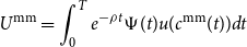 \begin{equation} U^{\textrm{mm}}=\int _{0}^{T}e^{-\rho t}\Psi (t) u(c^{\textrm{mm}}(t))dt \end{equation}
where $c^{\textrm{mm}}$
indicates the consumption an individual would experience if the shock hits at the date of retirement:
$c^{\textrm{mm}}$
indicates the consumption an individual would experience if the shock hits at the date of retirement:
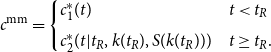 \begin{equation} c^{\textrm{mm}}= \begin{cases} c^*_1(t) & t\lt t_R\\[5pt] c^*_2(t|t_R,k(t_R),S(k(t_R))) & t\geq t_R. \end{cases} \end{equation}
The welfare effect of Social Security from the perspective of the policy maker is the fraction of lifetime consumption the individual would give up to participate in Social Security (given the individual hedged optimally, but the shock happened exactly at the date of retirement),
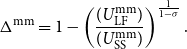 \begin{equation} \Delta ^{\textrm{mm}} =1-\left ( \frac{(U_{\textrm{LF}}^{\textrm{mm}})}{(U_{\textrm{SS}}^{\textrm{mm}})}\right ) ^{\frac{1}{1-\sigma }}. \end{equation}
We find the welfare effect of Social Security to be −2.28% using our baseline parameters and the uniform shock distribution. The welfare effect is less negative compared to the baseline, because the policy maker is only considering the worst possible shock date, rather than forming expected utility based on all possible shock dates. Social Security still reduces welfare because the internal rate of return is low compared to the risky asset—even when the shock hits at the worst possible moment.
However, the welfare effect is 3.55% using the exponential shock distribution. Social Security is welfare enhancing in this scenario because the individual optimally hedged risk under the assumption that the shock would only occur within their lifetime with probability 0.5, whereas the policy maker evaluates Social Security assuming the shock hits at the worst possible moment with probability 1.
Recall that the welfare effect of Social Security is −7.42% when the welfare criteria is calculated using expected utility [equation (27)] and the rare event risk is distributed exponentially. However, we have just shown, that if the welfare criteria is instead a maximin criteria—comparing utility of the worst possible realization of the shock rather than taking an expectation over all possible realizations of the shock—Social Security is welfare improving by the equivalent of 3.55%. In both cases, behavior is fully rational and the individual optimally hedges rare event risk. The only difference is which possible lifetime utility paths the policy maker includes in their welfare criteria. If all possible paths are included (and weighted according to the distribution of risk), Social Security is welfare reducing; however, if only the worst path is included, Social Security is welfare improving.
4. Inequality and redistribution
Our analysis thus far has focused on a representative (average) wage earner. In this section, we expand our analysis to consider Social Security’s safety net role in the presence of wage inequality.
We continue to hold the Social Security tax fixed at its statutory rate (10.6%), but now we consider different replacement rates. In actuality, the government computes the average of an individual’s highest 35 years of earnings and then calculates Social Security benefits as a piece-wise linear function of average earnings, with kinks or bend points at 0.2, 1.24, and 2.47 times the economy-wide mean wage. Social Security replaces 90% of an individual’s average wage up to 0.2 times the economy-wide mean wage, then replaces 32% of an individual’s average wage between 0.2 and 1.24 times the economy-wide mean wage, and finally replaces 15% of an individual’s average wage between 1.24 and 2.47 times the economy-wide wage. Wages beyond 2.47 times the economy-wide mean are not taxed and do not affect benefits. Hence, the lowest wage earners experience the highest replacement rate (90%), and the replacement rate is progressively less as wages increase beyond the first bend point.
We consider five different Social Security replacement rates that correspond to income quintiles. Our welfare results are presented in Table 3. Specifically, we assume that wages are distributed and Social Security benefits are calculated as in Cottle Hunt and Caliendo (Reference Cottle Hunt and Caliendo2022a) and calculate the replacement rate for the median earner for each earnings quintile. Then, we calculate the welfare effect of Social Security with our baseline uniform shock distribution (26) and with the alternative exponential shock distribution (28).
Table 3. Welfare effect of Social Security for the median earner of each income quintile, with optimal hedging and no hedging, for two different shock distributions
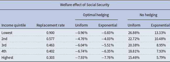
We calculate the welfare effect of Social Security assuming optimal hedging and find that Social Security makes individuals in all five earning quintiles worse off. Higher earners are harmed the most because Social Security benefits are progressive, and thus, high earners receive the lowest implicit rate of return.
Consider an individual with wages at or below the first bend point and hence a 90% replacement rate. Holding all other parameters fixed at the baseline calibration, the welfare effect of Social Security still is slightly negative. Intuitively, these individual’s experience a much higher internal rate of return on Social Security (4.4%), but this internal rate still is lower than most of the possible lifetime ex post rates of return on private saving. An individual who draws the very worst possible timing shock (at the moment of retirement) and losses 86% of their total accumulated wealth, effectively earns an ex post rate of return on their private saving of 3.75%. All other shock dates confer a higher rate of return on private saving than this. There is a specific window of time around the date of retirement for which the shock would need to hit in order for Social Security to outperform private saving, and this window is narrow enough that even a risk averse, low-income individual would prefer the risk-reward tradeoff found in private assets over participating in Social Security. Hence, even when making Social Security as attractive as possible by considering the highest possible replacement rate, while also assuming away any private options for insuring longevity risk, the performance of Social Security does not compare favorably to that of (risky) private assets.
We also calculate the welfare effect of Social Security assuming the individual does not hedge the rare event risk as in Section 3, and find that Social Security makes all groups better off with the largest welfare gains accruing to the lowest earners. These results are consistent with our earlier analysis: Social Security improves the ex ante expected utility of households who are unable to optimally hedge rare event risk by providing a safe asset.
In our model, Social Security provides direct insurance against longevity risk by paying retirement benefits as an annuity. In an ex ante sense, Social Security also provides insurance against having low lifetime earnings by using a progressive benefit earning rule. The welfare effects of Social Security are largest for individual’s with the lowest lifetime earnings.Footnote 12 Although our model does not include idiosyncratic wage shocks (like unemployment or periods of low earnings), Social Security would provide insurance against those shocks through the progressive benefit earning rule as well.Footnote 13
5. Discussion and limitations
Our analysis focuses on differences between households who optimally hedge rare event risk and those who fail to hedge. We find the ability of Social Security to function as a safety net (and improve ex ante expected utility) depends critically on whether or not the household hedges rare event risk. Our analysis includes two simplifications that likely have level effects on our welfare calculations. First, we assume the rare event shock happens at most once during a household’s life cycle. Second, we assume fixed factor prices.
5.1. One shock
The household in our model faces a risk of a rare event shock happening in their lifetime once (if the shock is distributed uniformly) or possibly not at all (if the shock is distributed exponentially). Of course, in reality, a household could experience a rare event shock that depresses the value of their assets multiple times. Modeling persistent or recurring shocks could amplify the insurance benefits of Social Security. In that sense, the welfare effects we find could be viewed as a lower bound.
From a conceptual standpoint, our single shock assumption has the disadvantage that the individual essentially enters a risk-free world after the shock hits, whereas in reality the individual still faces the risk that another rare shock might strike. This disadvantage is partially mitigated by two considerations. First, we focus on ex ante welfare and the individual faces the possibility of the shock hitting at any moment (or never) during the life cycle, which in turn creates a setting in which even a single shock has a powerful effect on welfare and decision making. Second, we have to allow the individual to get hit with multiple rare event shocks of the size of our calibrated shock (86% destruction of wealth with a 25-year recovery time), then we would be subjecting the individual to shocks that exceed the US experience over the last 100 years. While there have been multiple shocks over the last century (dot.com, Great Recession, etc), none of these shocks come close to the Great Depression in terms of relative loss in equity prices. In other words, while the individual only gets hit with one shock, it is a massive one.
Finally, our paper is an attempt to consider asset risk from a novel angle. Typically, returns on risky assets are modeled as random disturbances from a stationary distribution, without explicitly considering timing risk over very large rare shocks. We reverse this tradition by focusing on the latter and abstracting from the former. Of course, both risks are realistic but our focus on rare event risk is particularly relevant to our research question about safety nets.
5.2. Partial equilibrium
Second, we assumed exogenous factor prices. If we were to model a general equilibrium overlapping generations economy, the introduction of Social Security would crowd out private savings which would reduce the wage and increase the interest rate. These changes to factor prices would dampen the welfare effects of Social Security (if the economy was dynamically efficient). This channel has been well documented in Slavov et al. (Reference Slavov, Gorry, Gorry and Caliendo2019), Blau (Reference Blau2016), Conesa and Garriga (Reference Conesa and Garriga2008), and Kitao (Reference Kitao2014) among many others.
A full analysis of the welfare effect of Social Security would need a general equilibrium treatment of factor prices and bequest income, as Social Security affects the level of aggregate capital accumulation as well as the level of wealth that is transmitted across generations. In this paper, we do not attempt a full analysis of Social Security but instead attempt to clarify a single aspect of Social Security, and, in particular, to show the role of full optimization and full information. By showing that Social Security’s welfare effect can swing dramatically, from very negative to very positive as we move from full information/optimization to imperfections along these margins, we have identified some of the most significant modeling features that are of first-order importance to the research question.
Because we are specifically interested in the role of strong neoclassical assumptions like optimal hedging and full information in shaping our welfare conclusions, our partial equilibrium setting allows us to conveniently experiment with a number of different assumptions without needing to recalibrate to the larger macroeconomy and without needing to specify how the degree of optimizing behavior and information processing are distributed across households throughout the economy.
6. Conclusion
Social Security is the largest government program in existence and it affects Americans of all ages. Part of the initial rationale for creating Social Security in 1935 was to ensure that Americans are protected from financial shocks like the catastrophic stock market crash during the Great Depression. That particular shock was the worst shock to financial assets in the last 100 years, though more recent shocks such as the Great Recession and the COVID-19 pandemic have brought intense financial losses, especially to certain sectors of the economy, and have been particularly problematic for households who are close to retirement. While a large literature focuses on the welfare effects of Social Security, its role as a safety net against rare event risk to asset values has received less attention and is the purpose of our paper.
We build a model in which a rare but very large negative shock to financial wealth hits the household at an unknown time. The shock is especially painful if it occurs near retirement when the individual’s accumulated wealth is at a maximum. But since the timing of the shock is uncertain, individual’s must solve a dynamic stochastic life-cycle consumption and saving problem, and we utilize a recursive technique from the continuous-time control literature to obtain a closed-form solution. We calibrate the size of the shock to the Great Depression, which brought an 86% decline in equity values from peak to trough.
We consider a number of assumptions about the individual’s ability to hedge rare event risk and about the policy makers information. We find the answer to whether or not Social Security provides a safety net against rare event risk depends critically on these information and optimization assumption.
We show that if a household has full information on the distribution of rare event risk and solves a dynamic stochastic problem to hedge this risk by building up optimal precautionary savings balances, then Social Security is unnecessary as a safety net. Alternatively, if the household does not account for rare event risk in its financial planning and instead leaves itself exposed to rare shocks without a proper buffer, then Social Security can provide very large welfare gains as a safety net.


 Open access