


1. Introduction
Given the recent pandemic and similar global shocks such as the U.S. financial crisis, it is important to account for this information in a model that can identify unusual observations in variables with robust estimates. Harvey (Reference Harvey2013) discusses multivariate location models using a score-driven framework that models shocks using a Student t distribution. This approach emerges from works by Harvey (Reference Harvey2013) and Creal et al. (Reference Creal, Koopman and Lucas2013), which employ an observation-driven framework exploiting the information from the model’s score. Moreover, this approach is robust to unusual observations as a result of its nonlinear filters capable of accommodating extreme episodes in the data. In addition, Blasques et al. (Reference Blasques, Gorgi, Koopman and Wintenberger2018) as well as Blasques et al. (Reference Blasques, van Brummelen, Koopman and Lucas2022) derive invertibility conditions for the consistency and asymptotic normality of maximum likelihood estimators in these types of models, which minimizes the Kullback–Leibler divergence of the true and estimated filter values. This particular property of score-driven filters optimally utilizes the score information.
Harvey’s (Reference Harvey2013) multivariate location model is also known as a quasi-vector autoregressive (VAR) model [Blazsek et al. (Reference Blazsek, Escribano and Licht2020, Reference Blazsek, Escribano and Licht2022b)] since it allows a similar reduced form in comparison to VAR models. VAR models introduced by Sims (Reference Sims1980) are useful for macroeconomists who assess impulse response functions (IRFs) from monetary and fiscal policy shocks. However, high dimensional VAR models imply a large number of parameters to estimate, and adding factors to their structure emerges as a practical solution.
The principal contribution of this article is the addition of factors into QVAR score-driven models where the multivariate error term follows a Student t distribution. Factor components can capture relevant information from a large dataset of variables from several sectors of the economy. In this way, factor-augmented quasi-VAR (FAQVAR) models do not incorporate many variables explicitly and, at the same time, can address episodes of great disturbances. Given its score-driven dynamics, the FAQVAR model can be estimated using frequentist methods rather than Bayesian techniques.
The study of factors using macroeconomic variables starts with the work of Stock and Watson (Reference Stock and Watson2002). They show an improvement in forecasts for macroeconomic U.S. series using principal component methods. Bernanke et al. (Reference Bernanke, Boivin and Eliasz2005) incorporate factors following Stock and Watson’s (Reference Stock and Watson2002) principal component procedure in VAR dynamics when analyzing the effects of monetary policy, and also they jointly estimate factors and VAR models using Bayesian techniques. This model is used extensively in the literature because of its flexibility. For instance, Abbate et al. (Reference Abbate, Eickmeier, Lemke and Marcellino2016) estimate factor models by considering the financial crisis episode and its effects on greater economies while Laine (Reference Laine2020) assesses the effectiveness of monetary policy with a zero lower bound (ZLB) in the European Union.
I estimate FAQVAR models using the two-step procedure of Bernanke et al. (Reference Bernanke, Boivin and Eliasz2005), where in the first step the unobservable factors are obtained using principal component analysis, and then in the second step the estimated factors are added to the QVAR system. An alternative is the two-step maximum likelihood estimation undertaken by Bai, Li and Lu (Reference Bai, Li and Lu2016), who analyze inference properties of estimates and impulse responses for FAVAR models. However, I follow the two-step procedure of Bernanke et al. (Reference Bernanke, Boivin and Eliasz2005) and use Yamamoto’s (Reference Yamamoto2019) bootstrap strategy to deal with the uncertainty generated in the first step of the estimation of factors.
Dufour and Stevanović (Reference Dufour and Stevanović2013) utilize a bootstrap approach for their FAVAR moving average (FAVARMA) model and argue that the VARMA structure is able to capture the information from VAR models with long lags, so parsimonious. VARMA models allow similar impulse response estimates with considerably fewer parameters to estimate. The QVAR model collapses to a VARMA model with Gaussian errors when the degrees of freedom of the Student t distribution errors tend to infinity [Blazsek et al. (Reference Blazsek, Escribano and Licht2020)]. Therefore, a limiting case for the FAQVAR model is the FAVARMA model, which is the benchmark model in this study. In addition, Blazsek et al. (Reference Blazsek, Escribano and Licht2020) highlight that the QVAR specification can capture seasonal effects in IRFs.
Studies of the score-driven framework in macroeconomics include the work of Angelini and Gorgi (Reference Angelini and Gorgi2018), where they apply the score-driven approach to dynamic stochastic general equilibrium (DSGE) models with time-varying parameters and volatility. Additionally, Blazsek et al. (Reference Blazsek, Escribano and Licht2023b) establish score-driven representations with fat tails and heteroskedastic errors for DSGE models, while Blazsek et al. (Reference Blazsek, Escribano and Licht2023a) propose score-based cointegration models. Blazsek et al. (Reference Blazsek, Escribano and Licht2022a) propose a multivariate Markov-switching QVAR model, which allows for common trends and cointegration dynamics. In addition, Blazsek et al. (Reference Blazsek, Escribano and Licht2022b) develop a multivariate location plus scale model and derive its maximum likelihood conditions. These works constitute the first applications of the score-driven approach in macroeconomic systems that consider just a few variables in their composition. I extend this analysis to include factor-augmented variables that have not yet been studied in the literature and that this article aims to cover.
Recent literature dealing with observations from the pandemic includes the work of Lenza and Primiceri (Reference Lenza and Primiceri2022), who model the specific change in volatility during the pandemic within a VAR framework. Carriero et al. (Reference Carriero, Clark, Marcellino. and Mertens2021) treat the pandemic episode as outliers in their VAR model, which instead uses stochastic volatility errors following the approach of Stock and Watson (Reference Stock and Watson2016). Antolín-Díaz et al. (Reference Antolín-Díaz, Drechsel and Petrella2021) make a nowcasting analysis of the U.S economic activity with a dynamic factor model that also includes outliers.
Schorfheide and Song (Reference Schorfheide and Song2021) analyze the forecasts of a mixed-frequency VAR model and conclude that the model excluding pandemic data generates more accurate long-term forecasts. However, Hartwig (Reference Hartwig2021) and also Bobeica and Hartwig (Reference Bobeica and Hartwig2023) highlight the importance of modeling errors with a Student t distribution when the COVID-19 shock is considered in a VAR model, since the parameter estimates and density forecasts from a Gaussian version are sensitive to the pandemic data. All these works employ a Bayesian approximation for the estimation of their VAR models, whereas this article adopts an observation-driven approach, which can be estimated using frequentist methods.
In addition, Guerron-Quintana et al. (Reference Guerron-Quintana, Khazanov and Zhong2023) cover nonlinearities and asymmetries in state and measurement equations in VAR models using Bayesian estimation. The FAQVAR model proposed in this study is observation-driven with a closed-form likelihood that is estimated by maximum likelihood. Further, the FAQVAR model is robust to recently experienced extreme episodes such as the pandemic, given the modeling of errors as a Student t distribution. To the best of my knowledge, this article presents the first research considering the pandemic sample with a score-driven FAQVAR model.
I analyze the U.S. economy estimating the factor components using McCracken and Ng (Reference McCracken and Ng2016)’s macroeconomic monthly variables from January 1959 to May 2021, which cover tumultuous times for this market. Then, in the second step I estimate the model using the previously estimated factors and the federal funds rate (FFR) to evaluate monetary policy shocks. The FAQVAR model proposed in this study is robust to extreme episodes, including the recent pandemic, and it outperforms the FAVARMA model, producing a better fit to the data. The FAQVAR impulse response forecasts from a monetary shock follow the expected reactions from the economic theory. Additional robustness checks using different numbers of factors, a subsample before COVID-19, and the ZLB episodes indicate the stability of the estimates.
The structure of this article is as follows: Sections 2 and 3 discuss the structure of the FAQVAR model and its estimation, respectively. Section 4 presents the estimates in the application of the model to assess monetary policy in the U.S. economy. Section 5 checks the robustness of the estimates by estimating models with different numbers of factors, samples, and the unbounded shadow rate. The conclusions are presented in the last section.
2. Methodology
I incorporate factor components into the first-order QVAR model of Harvey (Reference Harvey2013) and Blazsek et al. (Reference Blazsek, Escribano and Licht2020). The model for a $y_{t}=(f_{t},x_{t})$
vector of
$y_{t}=(f_{t},x_{t})$
vector of $K=k+r$
variables contains the
$K=k+r$
variables contains the $k$
factors,
$k$
factors, $f_{t}$
, and the vector of
$f_{t}$
, and the vector of $r$
observed macroeconomic variables,
$r$
observed macroeconomic variables, $x_{t}$
, as follows:
$x_{t}$
, as follows:
 \begin{align} y_{t} & =c+\mu _{t}+\varepsilon _{t},\\ \nonumber \end{align}
 \begin{align} \mu _{t} & =\Phi \mu _{t-1}+\Psi u_{t-1},\\ \nonumber \end{align}
 \begin{align} z_{t} & =\Lambda _{f}f_{t}+\Lambda _{x}x_{t}+e_{t},\\ \nonumber \end{align}
 \begin{align} \varepsilon _{t} & \sim t_{\nu }(0,\Sigma ),\\ \nonumber \end{align}
 \begin{align} u_{t} & \varpropto \frac{\partial \ln f(y_{t}|Y_{t-1})}{\partial \mu _{t}}, \end{align}
where $c$
is a vector of constants,
$c$
is a vector of constants, $\mu _{t}$
is a location component with persistence
$\mu _{t}$
is a location component with persistence $\Phi$
,
$\Phi$
, $\Psi$
is the updating scale matrix from the score term component
$\Psi$
is the updating scale matrix from the score term component $u_{t}$
, and the vector of errors term
$u_{t}$
, and the vector of errors term $\varepsilon _{t}$
follows an independent and identically centered multivariate Student t distribution with scale
$\varepsilon _{t}$
follows an independent and identically centered multivariate Student t distribution with scale $\Sigma$
and
$\Sigma$
and $\nu \gt 2$
degrees of freedom. Following Bernanke et al. (Reference Bernanke, Boivin and Eliasz2005), I consider a set of
$\nu \gt 2$
degrees of freedom. Following Bernanke et al. (Reference Bernanke, Boivin and Eliasz2005), I consider a set of $Z$
informational variables for the estimation of factors, and each of these variables
$Z$
informational variables for the estimation of factors, and each of these variables $z_{t}$
is linked to the main observed variables with the linear representation, where
$z_{t}$
is linked to the main observed variables with the linear representation, where $\Lambda _{f}$
are the factor loadings with dimension
$\Lambda _{f}$
are the factor loadings with dimension $Z\times k$
,
$Z\times k$
, $\Lambda _{x}$
of dimension
$\Lambda _{x}$
of dimension $Z\times r$
is the effect of the observed economic variables on the informational dataset, and
$Z\times r$
is the effect of the observed economic variables on the informational dataset, and $e_{t}$
is the error term of this linear regression.
$e_{t}$
is the error term of this linear regression.
The multivariate scale matrix is positive definite so that $\Sigma =\Omega ^{-1}\Omega ^{-1\prime }$
can have a Cholesky decomposition which allows the identification of the model. The likelihood conditional on past information
$\Sigma =\Omega ^{-1}\Omega ^{-1\prime }$
can have a Cholesky decomposition which allows the identification of the model. The likelihood conditional on past information $Y_{t-1}=(y_{1},\ldots,y_{t})$
is given by
$Y_{t-1}=(y_{1},\ldots,y_{t})$
is given by
 \begin{align} \log f(y_{t}|Y_{t-1}) & =\log \Gamma \left ( \frac{\nu +K}{2}\right ) -\frac{K}{2}\log\!(\nu \pi )-\log \Gamma \left ( \frac{\nu }{2}\right ) -\frac{\log \left \vert \Sigma \right \vert }{2}\\ &\quad -\frac{\nu +K}{2}\log \left ( 1+\frac{\varepsilon _{t}^{\prime }\Sigma ^{-1}\varepsilon _{t}}{\nu }\right ) .\nonumber \end{align}
Finally, the score term $u_{t}$
is proportional to
$u_{t}$
is proportional to
 \begin{align} \frac{\partial \ln f(y_{t}|Y_{t-1})}{\partial \mu _{t}} & =\frac{\nu +K}{\nu }\Sigma ^{-1}\times \left ( 1+\frac{\varepsilon _{t}^{\prime }\Sigma ^{-1}\varepsilon _{t}}{\nu }\right ) ^{-1}\varepsilon _{t}, \end{align}
 \begin{align} & =\frac{\nu +K}{\nu }\Sigma ^{-1}\times u_{t}. \end{align}
3. Estimation
Factors are not observable, and accordingly, I first estimate these factors using the strategy of Bernanke et al. (Reference Bernanke, Boivin and Eliasz2005). The first step involves the estimation of factors that capture the main features from the informational variables $z_{t}$
. When evaluating monetary policy, we may consider indicators such as economic activity, stock markets, and inventories.
$z_{t}$
. When evaluating monetary policy, we may consider indicators such as economic activity, stock markets, and inventories.
I divide the group of informational variables based on whether or not each is contemporaneously affected by the monetary policy instrument $i_{t}$
.Footnote
1
Stock and Watson (Reference Stock and Watson2002) remark that the principal components from the informational dataset,
$i_{t}$
.Footnote
1
Stock and Watson (Reference Stock and Watson2002) remark that the principal components from the informational dataset, $\hat{C}_k(f_t,z_t)$
, may generate linear combinations of the policy instrument
$\hat{C}_k(f_t,z_t)$
, may generate linear combinations of the policy instrument $i_t$
when forecasted. To remove this effect, Bernanke et al. (Reference Bernanke, Boivin and Eliasz2005) consider the following regression:
$i_t$
when forecasted. To remove this effect, Bernanke et al. (Reference Bernanke, Boivin and Eliasz2005) consider the following regression:
 \begin{equation} \hat{C}_{k}(f_{t},z_{t})=\omega _{k}+a_{k}\hat{C}_{k}(f_{t})+b_{k}i_{t}+\xi _{kt}, \end{equation}
where $\hat{C}_{k}(f_{t})$
are the components from all non-contemporaneous variables,
$\hat{C}_{k}(f_{t})$
are the components from all non-contemporaneous variables, $\omega _{k}$
is an intercept,
$\omega _{k}$
is an intercept, $a_{k}$
and
$a_{k}$
and $b_{k}$
are elasticities, and
$b_{k}$
are elasticities, and $\xi _{kt}$
is an error term. The estimate for the factor components is given by
$\xi _{kt}$
is an error term. The estimate for the factor components is given by
 \begin{equation} \hat{f}_{kt}=\hat{\omega }_{k}+\hat{a}_{k}\hat{C}_{k}(f_{t},z_{t})+\hat{\xi }_{kt}. \end{equation}
The second estimation step consists of augmenting the QVAR system with the factors so that $y_{t}=(\hat{f}_{t},x_{t})$
. The FAQVAR model is estimated by maximizing the logarithm of the likelihood with respect to the parameter set
$y_{t}=(\hat{f}_{t},x_{t})$
. The FAQVAR model is estimated by maximizing the logarithm of the likelihood with respect to the parameter set $\psi =(\Phi,\Psi,\Sigma,\nu )$
:
$\psi =(\Phi,\Psi,\Sigma,\nu )$
:
 \begin{equation} \log L(\psi )=\sum _{t=1}^{T}\log f(y_{t}|Y_{t-1}). \end{equation}
Following Proposition 39 of Harvey (Reference Harvey2013), the maximum likelihood estimates are consistent since the score and the errors model are assumed to be identically and independently distributed. In addition, Harvey (Reference Harvey2013) and Blazsek and Licht (Reference Blazsek and Licht2020) establish conditions for the explicit derivation of the information matrix for the QVAR model standard error estimates. In contrast, I apply the non-parametric approach of Yamamoto (Reference Yamamoto2019) for the estimation of standard errors and IRFs of the FAQVAR model, which also capture the error estimation uncertainty from the first step.
3.1. Impulse response function
Blazsek et al. (Reference Blazsek, Escribano and Licht2020) establish the moving average representation of the stationary process $\mu _{t}$
, provided its persistence
$\mu _{t}$
, provided its persistence $\Phi$
has a modulus
$\Phi$
has a modulus $\lambda$
less than one in equation (2). The MA form is
$\lambda$
less than one in equation (2). The MA form is
 \begin{equation} \mu _{t}=\sum _{h=1}^{\infty }\Phi ^{h}\Psi \lbrack (\nu -2)\nu ]^{1/2}\Omega ^{-1}\frac{\epsilon _{t-1-h}}{\nu -2+\epsilon _{t-1-h}^{\prime }\epsilon _{t-1-h}}, \end{equation}
with $\epsilon _{t}$
being the error term for the MA representation of the FAQVAR model,
$\epsilon _{t}$
being the error term for the MA representation of the FAQVAR model,
 \begin{equation} \epsilon _{t}=\left [ \frac{\nu }{\nu -2}\right ] ^{-1/2}\Omega \times \varepsilon _{t}. \end{equation}
The impulse responses for the shock $\epsilon _{t}$
at the horizon
$\epsilon _{t}$
at the horizon $j=1,\ldots,\infty$
to the variable
$j=1,\ldots,\infty$
to the variable $y_{t}$
are given by
$y_{t}$
are given by
 \begin{align} \hat{\Theta }_{j} & =E\left [ \frac{\partial y_{t+j}}{\partial \epsilon _{t}}\right ], \end{align}
 \begin{align} &\qquad\quad =\Phi ^{j}\Psi \lbrack (\nu -2)\nu ]^{1/2}\Omega ^{-1}E[D_{t-1-j}], \end{align}
where
 \begin{equation} D_{t}=\left [ \displaystyle\begin{array}[c]{cccc} \displaystyle\frac{\nu -2+\epsilon _{t}^{\prime }\epsilon _{t}-2\epsilon _{1t}^{2}}{(\nu -2+\epsilon _{t}^{\prime }\epsilon _{t})^{2}} & \displaystyle\frac{-2\epsilon _{1t}\epsilon _{2t}}{(\nu -2+\epsilon _{t}^{\prime }\epsilon _{t})^{2}} & \displaystyle\ldots & \displaystyle\frac{-2\epsilon _{1t}\epsilon _{Kt}}{(\nu -2+\epsilon _{t}^{\prime }\epsilon _{t})^{2}}\\[6pt] \displaystyle\frac{-2\epsilon _{2t}\epsilon _{1t}}{(\nu -2+\epsilon _{t}^{\prime }\epsilon _{t})^{2}} & \displaystyle\frac{\nu -2+\epsilon _{t}^{\prime }\epsilon _{t}-2\epsilon _{2t}^{2}}{(\nu -2+\epsilon _{t}^{\prime }\epsilon _{t})^{2}} & \displaystyle\ldots & \displaystyle\ldots \\[6pt] \displaystyle\ldots & \displaystyle\ldots & \displaystyle\ldots & \displaystyle\ldots \\[6pt] \displaystyle\frac{-2\epsilon _{Kt}\epsilon _{1t}}{(\nu -2+\epsilon _{t}^{\prime }\epsilon _{t})^{2}} & \displaystyle\ldots & \displaystyle\ldots & \displaystyle\frac{\nu -2+\epsilon _{t}^{\prime }\epsilon _{t}-2\epsilon _{Kt}^{2}}{(\nu -2+\epsilon _{t}^{\prime }\epsilon _{t})^{2}}\end{array} \right ]. \end{equation}
The expectation in (14) can be obtained considering the time average of $D_{t}$
. The impulse responses to the full description of informational variables come from the regression in (8) since
$D_{t}$
. The impulse responses to the full description of informational variables come from the regression in (8) since
 \begin{align} \hat{z}_{t} & =\hat{\Lambda }_{f}\hat{f}_{t}+\hat{\Lambda }_{x}x_{t}, \end{align}
 \begin{align} & =\left [ \begin{array}[c]{cc} \displaystyle\hat{\Lambda }_{f} & \hat{\Lambda }_{x}\end{array} \right ] \left [ \begin{array} [c]{c} \displaystyle\hat{f}_{t}\\ \displaystyle x_{t}\end{array} \right ], \end{align}
 \begin{align} & =\hat{\Lambda }y_{t}^{\prime }, \end{align}
 \begin{align} & =\hat{\Lambda }\left [ c+\Phi \mu _{t-1}+\Psi u_{t-1}+\varepsilon _{t}\right ] ^{\prime }. \end{align}
For the estimation of standard errors and impulse responses, I follow the residual approach of Yamamoto (Reference Yamamoto2019). This bootstrap method deals with the 2-step estimation errors from the pre-estimation of factors of Bernanke et al. (Reference Bernanke, Boivin and Eliasz2005). Dufour and Stevanović (Reference Dufour and Stevanović2013) adapts Yamamoto’s (Reference Yamamoto2019) algorithm for a FAVARMA model, which is the limiting case of the first-order FAQVAR model. The score-driven framework assumes that the second moments for the score and errors are finite and normally distributed as in Yamamoto’s (2019) bootstrap method, and then we can modify the linear algorithm to the FAQVAR model with the following steps:
-
1. Obtain the parameter estimates $\hat{c}$
,
$\hat{\Phi }$
,
$\hat{\Psi }$
,
$\hat{\Sigma }$
,
$\hat{\nu }$
,
$\hat{\Lambda }_{f}$
, and
$\hat{\Lambda }_{y}$
from the model in (1) along with their respective residuals
$\hat{\varepsilon }_{t}$
and
$\hat{e}_{t}$
. Estimate the impulse responses
$\hat{\Theta }_{i,j},$
and the IRFs for the augmented model determined by
$\hat{\Lambda }$
.
$\hat{c}$
,
$\hat{\Phi }$
,
$\hat{\Psi }$
,
$\hat{\Sigma }$
,
$\hat{\nu }$
,
$\hat{\Lambda }_{f}$
, and
$\hat{\Lambda }_{y}$
from the model in (1) along with their respective residuals
$\hat{\varepsilon }_{t}$
and
$\hat{e}_{t}$
. Estimate the impulse responses
$\hat{\Theta }_{i,j},$
and the IRFs for the augmented model determined by
$\hat{\Lambda }$
. -
2. Proceed with sampling residuals with replacement to generate
$\varepsilon _{t}^{\ast }$
and
$e_{t}^{\ast }$
for the bootstrapped samples
$y_{t}^{\ast }$
so that(21)
\begin{align} y_{t}^{\ast } & =\hat{c}+\mu _{t}^{\ast }+\varepsilon _{t}^{\ast }, \end{align}
(22)
\begin{align} \mu _{t}^{\ast } & =\hat{\Phi }\mu _{t-1}^{\ast }+\hat{\Psi }u_{t-1}^{\ast }, \end{align}
(23)
\begin{align} z_{t}^{\ast } & =\hat{\Lambda }_{f}f_{t}^{\ast }+\hat{\Lambda }_{y}x_{t}^{\ast }+e_{t}^{\ast }. \end{align}
-
3. Estimate the two-step system with
$y_{t}^{\ast }$
and obtain the bootstrapped parameter estimates
$\hat{c}^{\ast }$
,
$\hat{\Phi }^{\ast }$
,
$\hat{\Psi }^{\ast }$
,
$\hat{\Sigma }^{\ast }$
,
$\hat{\nu }^{\ast }$
,
$\hat{\Lambda }_{f}^{\ast }$
,
$\hat{\Lambda }_{y}^{\ast }$
, and the bootstrapped impulse responses
$\hat{\Theta }_{i,j}^{\ast }.$
-
4. Repeat steps 2–3
$R$
times. -
5. Compute the bootstrapped standard errors for model parameters.
-
6. Sort the bootstrapped impulse responses from the centered statistic
$s_{i,j}=\hat{\Theta }_{i,j}^{\ast }-\hat{\Theta }_{i,j}$
, select the significance level
$\alpha$
to obtain the confidence interval
$[\hat{\Theta }_{i,j}-s^{1-\alpha/2},\hat{\Theta }_{i,j}-s^{\alpha/2}],$
where
$s^{1-\alpha/2}$
and
$s^{\alpha/2}$
are
$1-\alpha/2$
and
$\alpha/2$
percentiles, respectively.


4. Empirical results
I use 128 variables from the McCracken and Ng (Reference McCracken and Ng2016) dataset that spans 1959:01 to 2021:05. I screen the data for observations associated with input errors and events such as labor strikes as noted by Stock and Watson (Reference Stock and Watson2002) assuming these observations are greater than 10 times their interquartile range.Footnote
2
In addition, I employ their expectation maximization algorithm to replace the missing and the screened values in the standardized panel data. The panel contains the FFR and a group of informational variables $z_{t}$
with indicators for output and income, the labor market, consumption, housing starts and sales, inventories and orders, the stock market, exchange rates, interest rates, money and credit, prices, as well as average hourly earnings and the consumer index. Further details for all variables are given in the Supplementary Material.Footnote
3
$z_{t}$
with indicators for output and income, the labor market, consumption, housing starts and sales, inventories and orders, the stock market, exchange rates, interest rates, money and credit, prices, as well as average hourly earnings and the consumer index. Further details for all variables are given in the Supplementary Material.Footnote
3
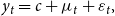
I estimate the first 10 factors using principal components as in Bernanke et al. (Reference Bernanke, Boivin and Eliasz2005), and a preliminary scree plot provides evidence of the contribution of each component to the total variance. Figure 1 shows this decomposition.
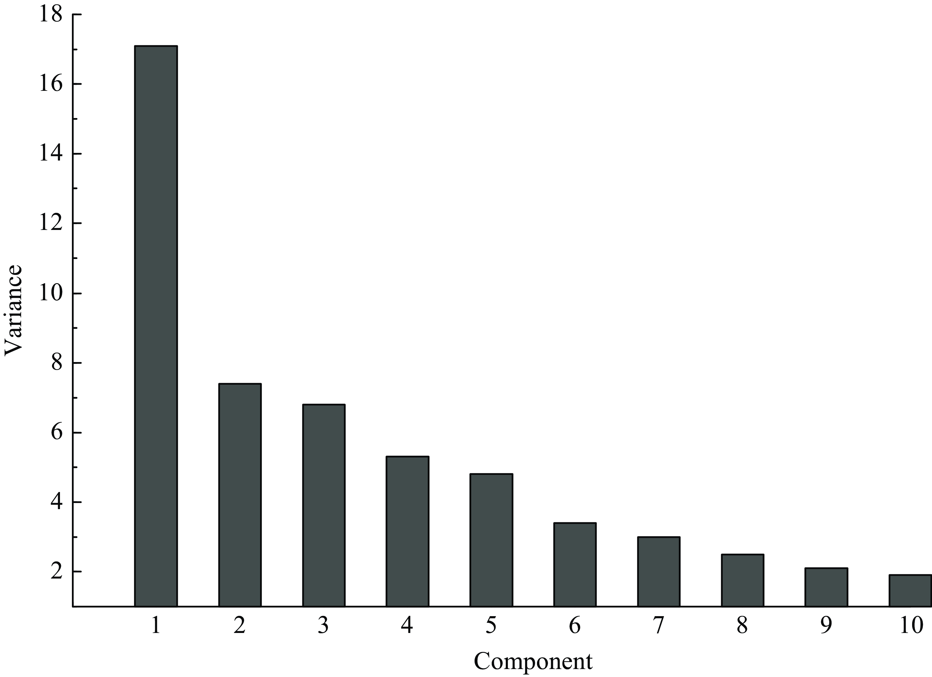
Figure 1. Scree plot.
Jointly, these 10 components contribute 54.4% of the explained variance of the data. The first, second, third, and fourth components explain 17.1, 7.4, 6.8, and 5.3% of the total variance, respectively, and the other factors contribute smaller amounts of less than 5% each. Bai and Ng (Reference Bai and Ng2002) propose information criteriaFootnote 4 for the optimal selection of factors in a dynamic factor model and I consider the following three criteria:
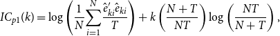 \begin{align} \textit{IC}_{p1}(k) & =\log \left ( \frac{1}{N}{\displaystyle \sum \limits _{i=1}^{N}}\frac{\hat{e}_{ki}^{\prime }\hat{e}_{ki}}{T}\right ) +k\left ( \frac{N+T}{NT}\right ) \log \left ( \frac{NT}{N+T}\right ), \end{align}
 \begin{align} \textit{IC}_{p2}(k) & =\log \left ( \frac{1}{N}{\displaystyle \sum \limits _{i=1}^{N}}\frac{\hat{e}_{ki}^{\prime }\hat{e}_{ki}}{T}\right ) +k\left ( \frac{N+T}{NT}\right ) \log\!\left ( \min\![N,T]\right ), \end{align}
 \begin{align} \textit{IC}_{p3}(k) & =\log \left ( \frac{1}{N}{\displaystyle \sum \limits _{i=1}^{N}}\frac{\hat{e}_{ki}^{\prime }\hat{e}_{ki}}{T}\right ) +k\frac{\log\!\left ( \min\![N,T]\right ) }{\min\![N,T]}, \end{align}
where $k$
is the number of factors,
$k$
is the number of factors, $N=K-1$
since the FFR is not considered directly in the estimation of factors, and
$N=K-1$
since the FFR is not considered directly in the estimation of factors, and $\hat{e}_{ki}$
are the residuals from the estimate of a dynamic factor model assuming
$\hat{e}_{ki}$
are the residuals from the estimate of a dynamic factor model assuming $k$
factors. I evaluate the criteria using the first 10 components, and Table 1 presents their values.
$k$
factors. I evaluate the criteria using the first 10 components, and Table 1 presents their values.
The first two criteria suggest eight factors, while the last criterion indicates 10 factors.Footnote 5 I chose the model with eight factors as the main model. I estimate these eight factors using principal components following Bernanke et al. (Reference Bernanke, Boivin and Eliasz2005).
Table 1. Bai and Ng (2002) number of factors criteria

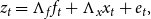
Factors 1 and 2 capture most of the variance according to the principal components methodology. In addition, in Figure 2, we can see the atypical observations and outliers generated after 2005 associated primarily with the U.S. financial crisis, the pandemic and other turbulent episodes since 1959.
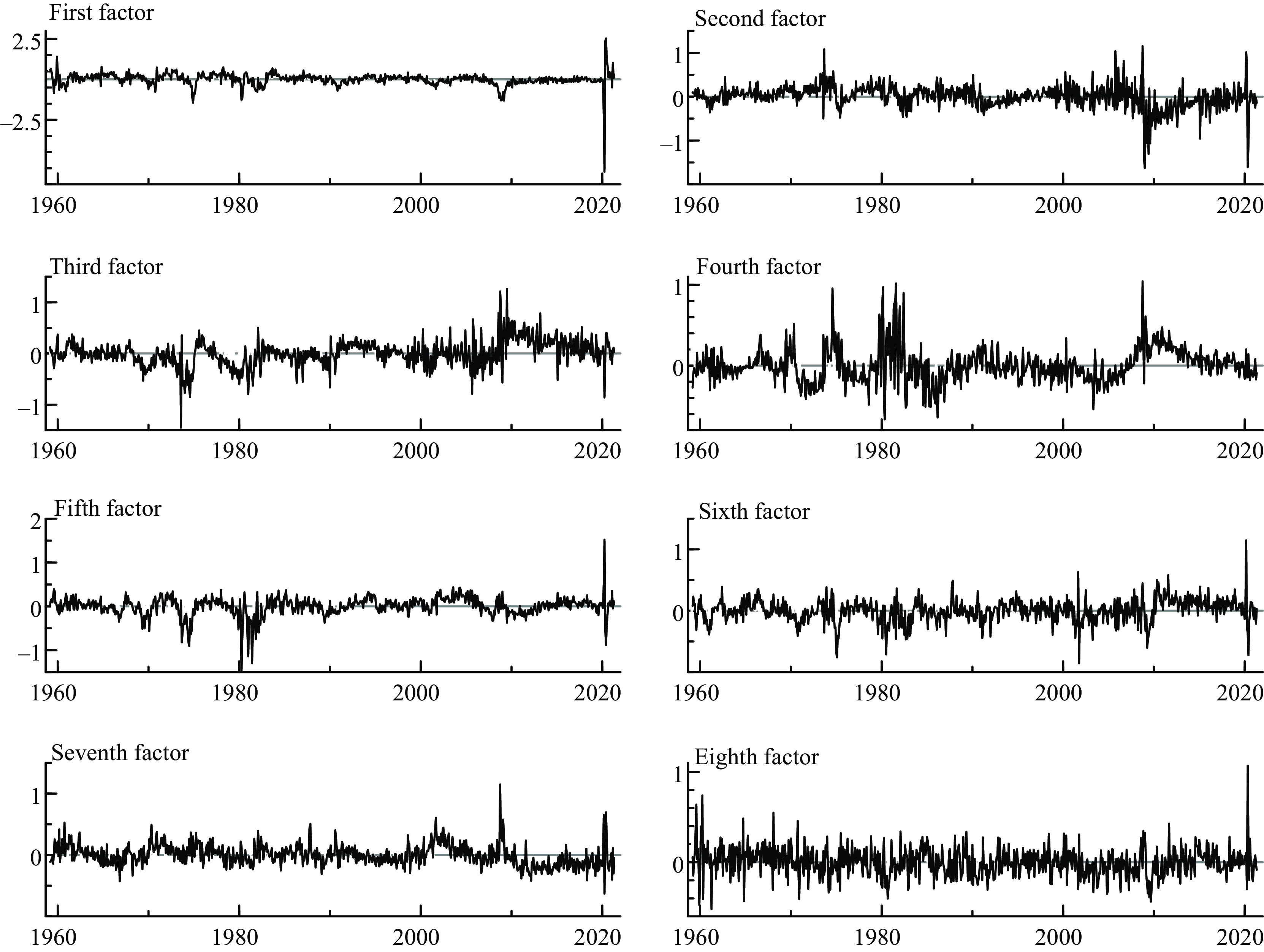
Figure 2. Factor estimates.
I analyze a FAQVAR model using eight factors chosen according to Bai and Ng (Reference Bai and Ng2002)’s criteria, and these factors are able to capture the large variability of the data, especially during the U.S. financial crisis and the pandemic. Hence, the dependent variables comprise nine variables ordered from the first factor to the eighth as well as the FFR. I also estimate the limiting FAVARMA Gaussian model of Dufour and Stevanović (Reference Dufour and Stevanović2013) when
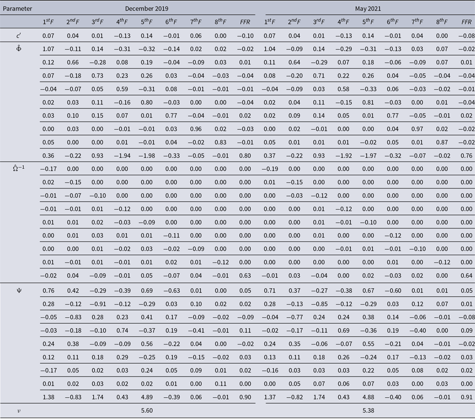
 $\nu \rightarrow \infty .$
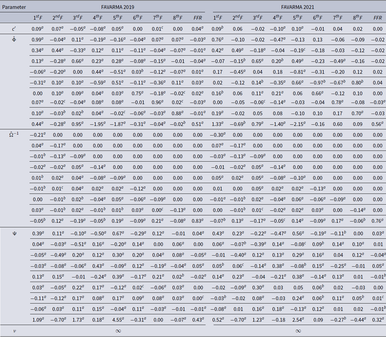
Table 2 reports the FAVARMA and FAQVAR model estimates, with each column containing estimates for one of the nine dependent variables.Footnote
6
$\nu \rightarrow \infty .$
Table 2 reports the FAVARMA and FAQVAR model estimates, with each column containing estimates for one of the nine dependent variables.Footnote
6
Table 2. FAVARMA and FAQVAR models estimates
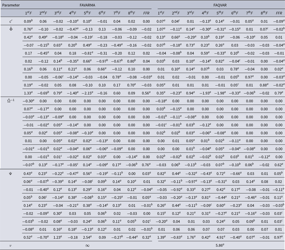
Notes: $^{a}$
,
$^{a}$
, $^{b}$
, and
$^{b}$
, and $^{c}$
denote residual bootstrapping significance at
$^{c}$
denote residual bootstrapping significance at $1\%$
,
$1\%$
, $5\%$
, and
$5\%$
, and $10\%$
, respectively. The model is
$10\%$
, respectively. The model is $y_{t}=c+\mu _{t}+\varepsilon _{t},$
where
$y_{t}=c+\mu _{t}+\varepsilon _{t},$
where $\mu _{t}=\Phi \mu _{t-1}+\Psi u_{t-1}$
and
$\mu _{t}=\Phi \mu _{t-1}+\Psi u_{t-1}$
and $\varepsilon _{t}\sim t_{\nu }(0,\Omega ^{-1}\Omega ^{-1\prime })$
.
$\varepsilon _{t}\sim t_{\nu }(0,\Omega ^{-1}\Omega ^{-1\prime })$
. $F$
and
$F$
and $FFR$
denote factor and federal funds rate, respectively.
$FFR$
denote factor and federal funds rate, respectively.
The persistence estimates of the FAQVAR model in matrix $\hat{\Phi }$
are generally higher than the FAVARMA values, and the estimates for the impact matrix
$\hat{\Phi }$
are generally higher than the FAVARMA values, and the estimates for the impact matrix $\hat{\Omega }^{-1}$
are lower for the FAQVAR model. This might be explained because the degrees of freedom capture (to some extent) the impact from shocks. In addition, the entries for the updating matrix
$\hat{\Omega }^{-1}$
are lower for the FAQVAR model. This might be explained because the degrees of freedom capture (to some extent) the impact from shocks. In addition, the entries for the updating matrix $\hat{\Psi }$
are more pronounced relative to those of the FAVARMA specification.
$\hat{\Psi }$
are more pronounced relative to those of the FAVARMA specification.
Table 3 presents the model diagnostics that allow assessment of stationary conditions and fit to the data. Both systems are stable given that for both models the maximum eigenvalues of $\hat{\Phi }$
are
$\hat{\Phi }$
are $0.958$
and
$0.958$
and $0.994$
in modulus. In addition, Blazsek et al. (Reference Blazsek, Escribano and Licht2023a) provide conditions to ensure that the QVAR model is stationary and ergodic, which also apply to the FAQVAR specification.
$0.994$
in modulus. In addition, Blazsek et al. (Reference Blazsek, Escribano and Licht2023a) provide conditions to ensure that the QVAR model is stationary and ergodic, which also apply to the FAQVAR specification.
Table 3. FAVARMA and FAQVAR model diagnostics
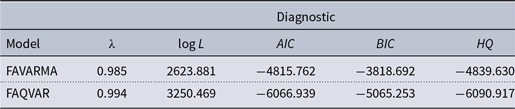
Notes: $\lambda$
is the maximum eigenvalue for the persistence matrix
$\lambda$
is the maximum eigenvalue for the persistence matrix $\hat{\Phi }$
.
$\hat{\Phi }$
. $AIC$
,
$AIC$
, $BIC$
, and
$BIC$
, and $HQ$
are the Akaike, Bayesian, and Hannan and Quinn information criteria, respectively.
$HQ$
are the Akaike, Bayesian, and Hannan and Quinn information criteria, respectively.
There are important gains in the in-sample fit to the data from the likelihood values and the Akaike (Reference Akaike1974) information, Bayesian information [Schwarz (Reference Schwarz1978)], and Hannan and Quinn (Reference Hannan and Quinn1979) criteria when I consider the score-driven approach. The estimate of the degrees of freedom is small and the addition of this parameter to the model is statistically significant, this means that the FAQVAR model is able to capture the atypical observations in the panel data.
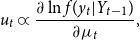
After the estimation of parameters and factor loadings, I produce and plot the impulse responsesFootnote
7
to a one standard-deviation contractionary monetary shock, or equivalently to a 116 basis points rise in the FFR,Footnote
8
as shown in Figure 3. I evaluate the impacts of some relevant economic variables after scaling them in levels, although all impulse responses can be reproduced from the informational set $z_{t}$
employing the estimates of equations (14) and (19). As in Yamamoto (Reference Yamamoto2019), the variables considered for analysis are: industrial production index, consumer price index, the exchange rate of Yen to U.S. dollar, the civilian unemployment rate, and new orders for durable goods. The dotted 95% confidence bands are obtained using 1000 residual bootstrap iterations.Footnote
9
$z_{t}$
employing the estimates of equations (14) and (19). As in Yamamoto (Reference Yamamoto2019), the variables considered for analysis are: industrial production index, consumer price index, the exchange rate of Yen to U.S. dollar, the civilian unemployment rate, and new orders for durable goods. The dotted 95% confidence bands are obtained using 1000 residual bootstrap iterations.Footnote
9
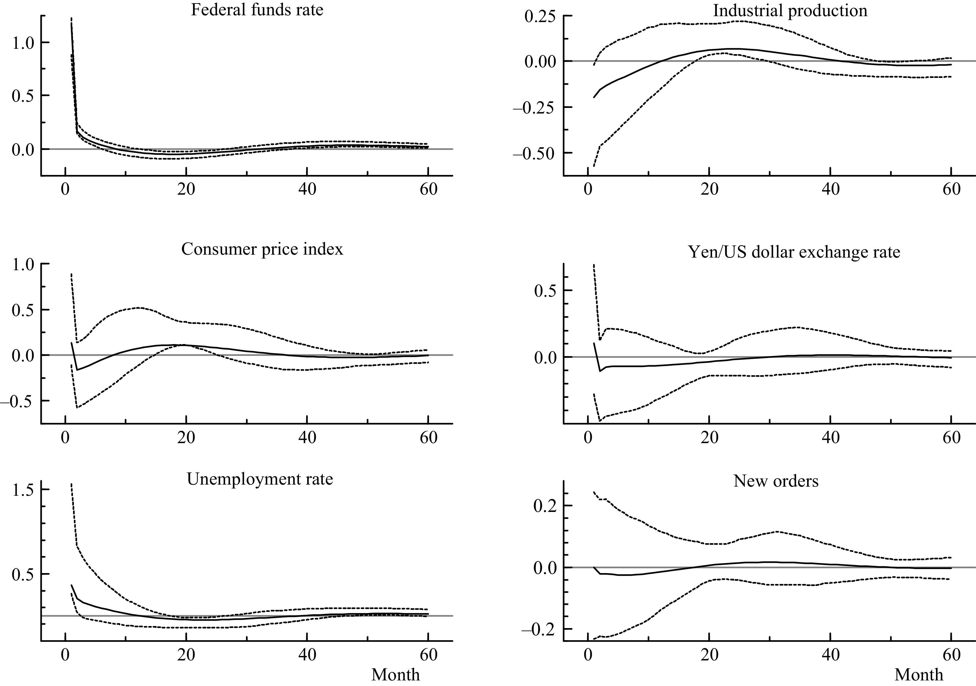
Figure 3. Impulse responses from a contractionary monetary policy shock.
Note: Impulse responses from the FAQVAR model with eight factors, with 95% confidence intervals in dotted lines.
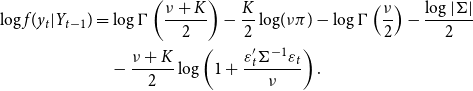
Figure 4 displays a comparison between responses to contractionary monetary policy shocks implied by the FAVARMA and FAQVAR models. The responses from the FAVARMA model are influenced by crash periods during the global financial crisis and the pandemic that distorted the effects on the consumer price index, exchange rate, and new orders, this generates a greater decay during the first months relative to the responses from the FAQVAR model. In comparison to the FAVARMA model, the FAQVAR model effects on new durable goods orders are smoother and more conservative. Moreover, the confidence intervals for most of the variables are wider in the first months after the shock when considering the linear model as reported in Figure A1 in the Supplementary Material. This reveals a greater uncertainty generated by multiple shocks that are not captured in the FAVARMA specification.
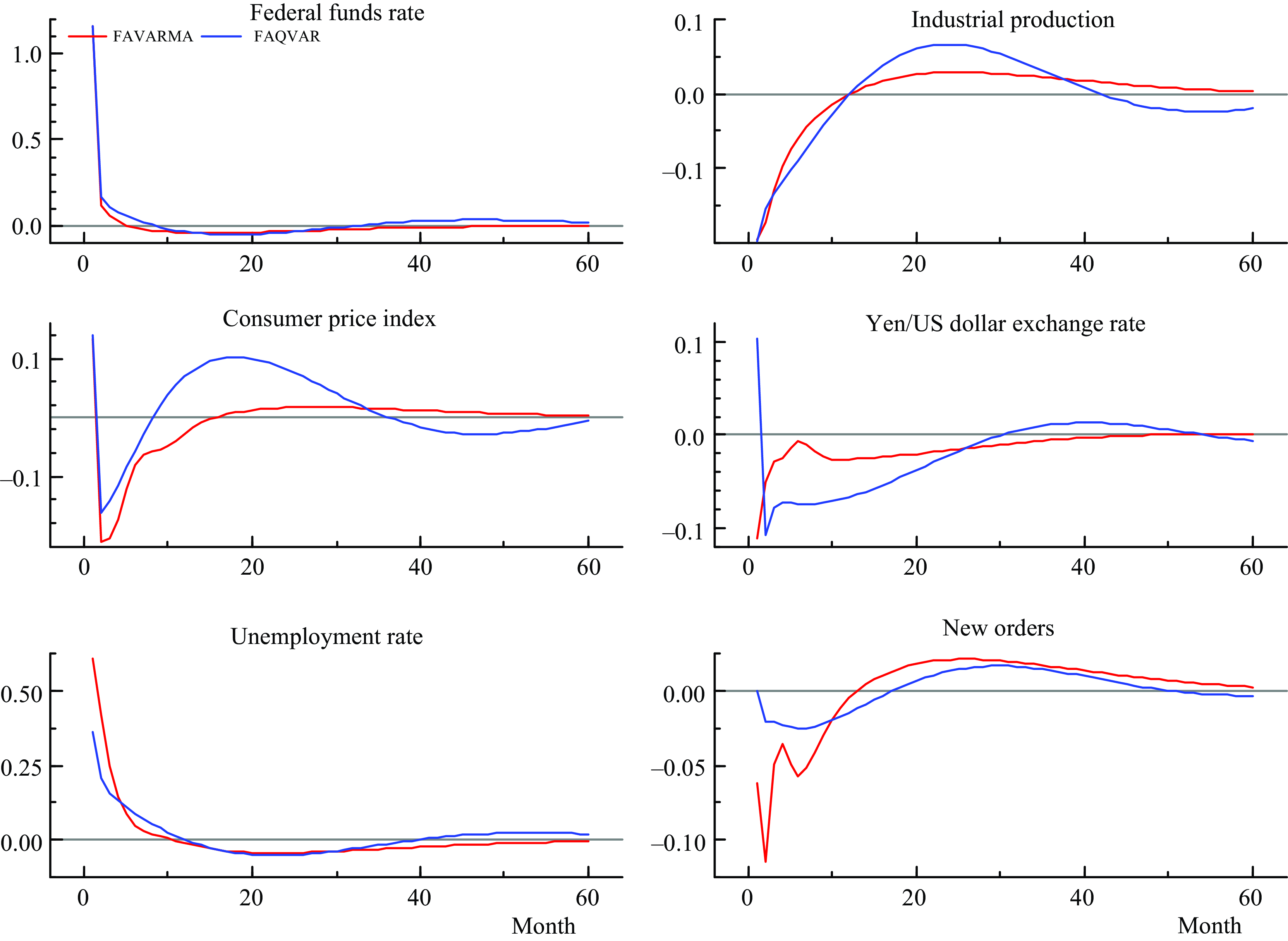
Figure 4. Impulse responses from a contractionary monetary policy shock: FAVARMA and FAQVAR.
Note: Impulse responses in months from FAVARMA and FAQVAR models with eight factors.
As expected from the proposed nonlinear model, the responses from the FAQVAR model generate hump shapes that raise the effect on the consumer price index and industrial production as soon as the interest rate reaches negative territory.Footnote 10 In particular, the higher hump-shaped reaction that starts at the 9th month might have originated from the quantitative easing policies during the financial crisis and pandemic, which aimed to boost economic activity.
Further, the FAQVAR model captures the turbulent episodes as atypical since it is modeled with a heavy tail distribution. The impulse responses follow the expected pattern when a contractionary monetary shock occurs: a decrease in industrial production, a decline in prices, a rise in the unemployment rate, a reduction in the number of orders, and an increase in the Yen/Dollar exchange rate. The FAVAR model estimates of Bernanke et al. (Reference Bernanke, Boivin and Eliasz2005) and the FAVARMA model of Dufour and Stevanović (Reference Dufour and Stevanović2013) find similar patterns for a sample that extends until 2005 which did not include last turbulent episodes.
5. Alternative specifications
In this section, I estimate additional models with different numbers of factors to verify the robustness of the estimates in the FAQVAR model. I also estimate the model using a subsample that does not include the pandemic period. Figure 5 shows the IRFs from models that consider two, four, and six augmented factors.
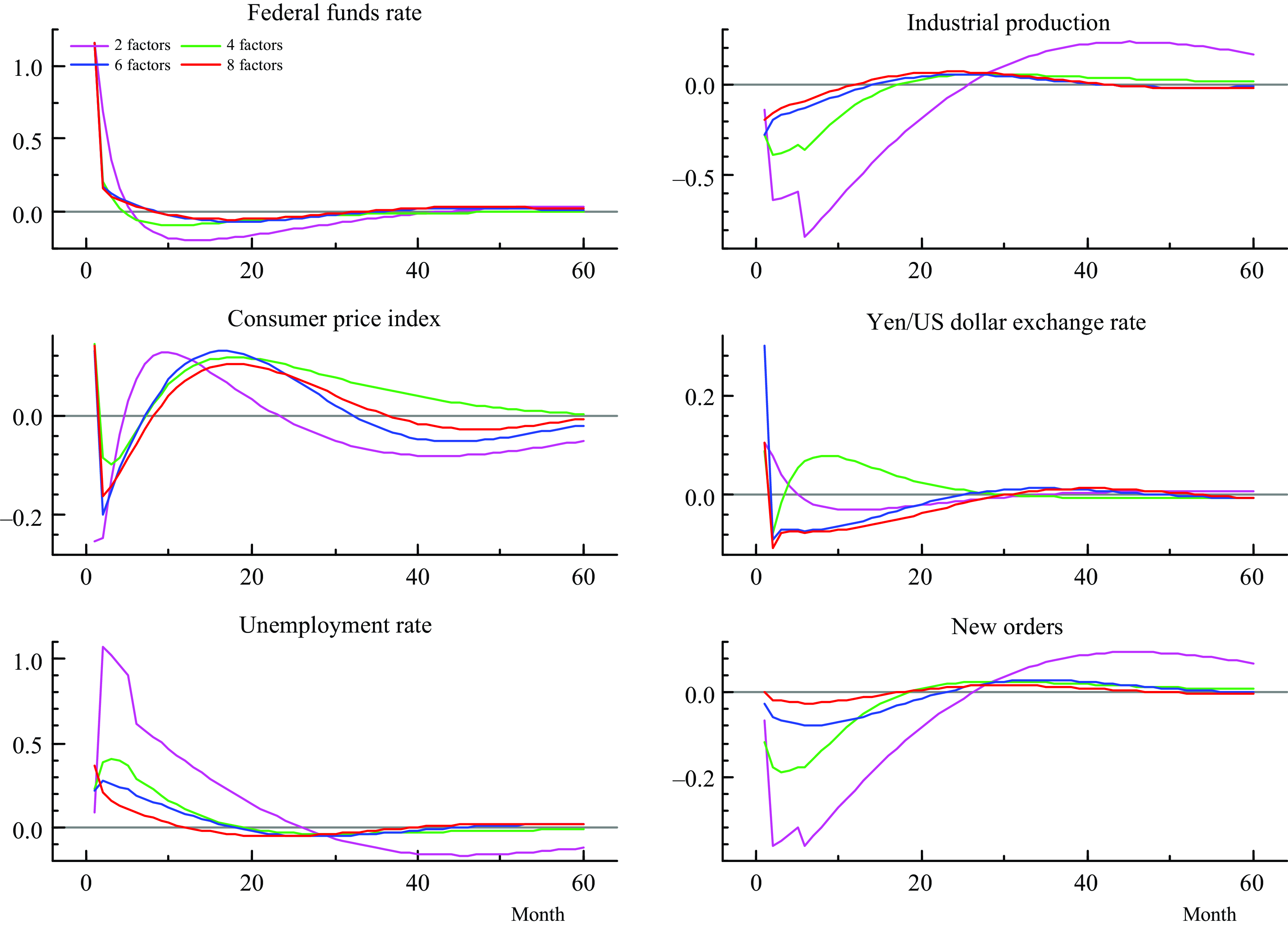
Figure 5. Impulse responses from a contractionary monetary policy shock and different number of factors.
We can observe that the impacts derived from a model that only considers two factors are bigger and exhibit some breaks in industrial production, unemployment rate, and new orders. As the dimension increases the responses are smoother in general. The paths of the shocks are similar in all scenarios except for the reaction of the exchange rate when four factors are used. However, because the model incorporates more information from the components the responses become quite similar, as when we compare the figures for six and eight factors, for instance. This may suggest informational sufficiency from the informational variables [Forni and Gambetti (Reference Forni and Gambetti2014)].
5.1. Estimates before and during COVID-19
I provide an additional robustness check by comparing the subsample up to the end of 2019 before the declaration of the COVID-19 pandemic and the full sample that takes the pandemic into account. As a benchmark exercise, Table 4 shows the estimates from the Gaussian FAVARMA model for both samples. We can see the effect of the pandemic on the estimates of the FAVARMA linear model, mainly affecting the estimates associated with the first factor. This means that a Gaussian assumption in times of high uncertainty can have severe effects on the linear model and policy assessment since the model does not accommodate extreme observations in comparison to a heavy tail distribution.
In contrast, the estimates and impulse responses from the FAQVAR model with a Student t distribution are almost identical for both samples. Figure 6 exhibits the impulse responses from factors and monetary shocks to their same variables. The responses are identical for the subsample until December 2019 and the full sample until May 2021. There are a couple of points to highlight: first that the estimates of the FAQVAR model are robust to unprecedented behavior of variables during the pandemic, and second, that the estimates are stable given that the trajectory of the responses is almost the same.
Table 4. FAVARMA models estimates
Notes: $^{a}$
,
$^{a}$
, $^{b}$
, and
$^{b}$
, and $^{c}$
denote residual bootstrapping significance at
$^{c}$
denote residual bootstrapping significance at $1\%$
,
$1\%$
, $5\%$
, and
$5\%$
, and $10\%$
, respectively. The model is
$10\%$
, respectively. The model is $y_{t}=c+\mu _{t}+\varepsilon _{t},$
where
$y_{t}=c+\mu _{t}+\varepsilon _{t},$
where $\mu _{t}=\Phi \mu _{t-1}+\Psi u_{t-1}$
and
$\mu _{t}=\Phi \mu _{t-1}+\Psi u_{t-1}$
and $\varepsilon _{t}\sim t_{\nu }(0,\Omega ^{-1}\Omega ^{-1\prime })$
.
$\varepsilon _{t}\sim t_{\nu }(0,\Omega ^{-1}\Omega ^{-1\prime })$
. $F$
and
$F$
and $FFR$
denote factor and federal funds rate, respectively.
$FFR$
denote factor and federal funds rate, respectively.
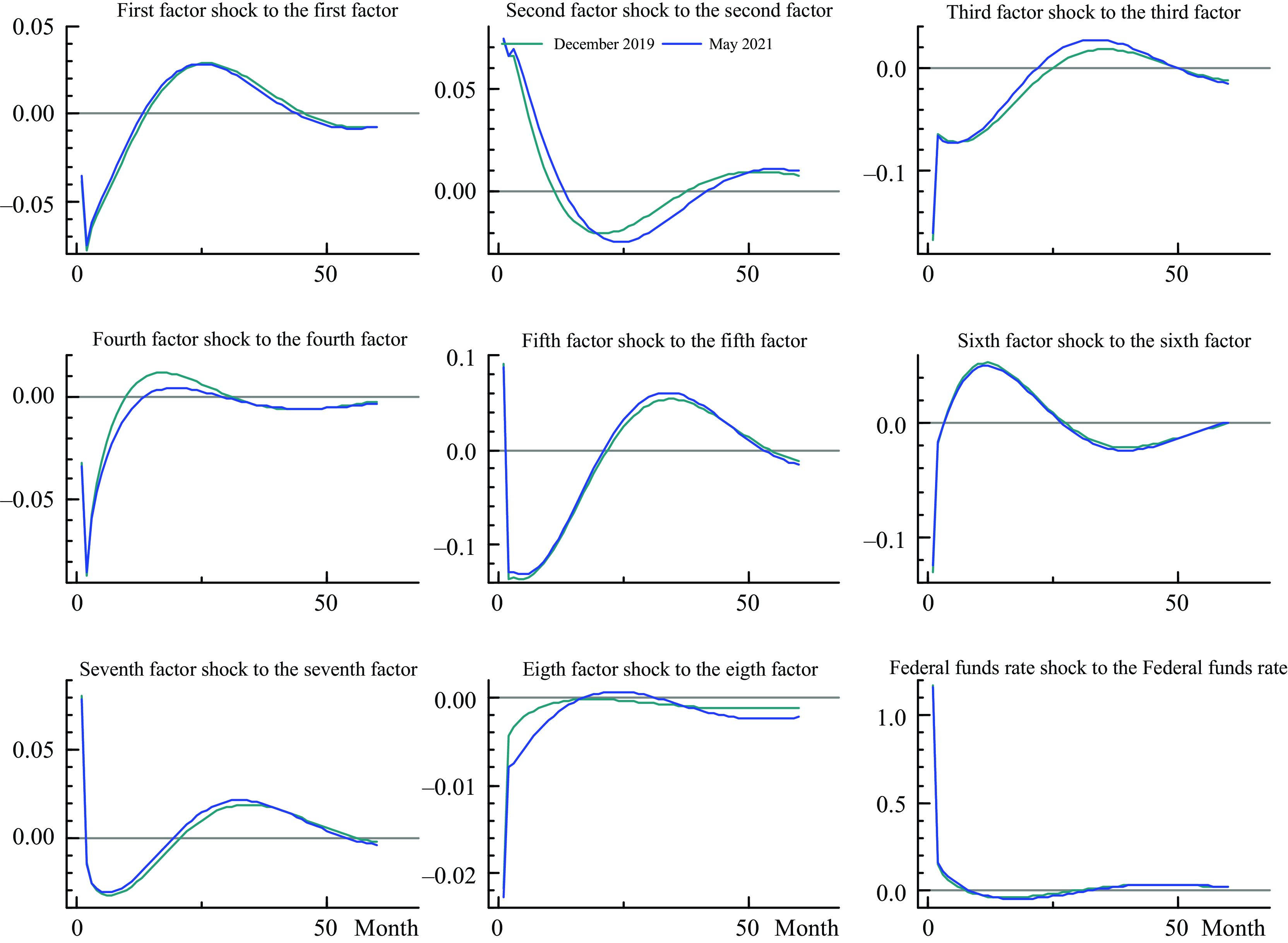
Figure 6. Impulse responses from factors and monetary policy shocks.
In Table 5, I report the bootstrap mean estimates from the FAQVAR models using the subsample until December 2019, and the full sample. In line with the findings of Bobeica & Hartwig (Reference Bobeica and Hartwig2023), the average of the degrees of freedom estimates supports the model with heavy tails before and after COVID-19 with a slightly lower average when considering the pandemic period.Footnote 11 Further, the intercept vector, persistence, and updating matrices display similar entries across both samples.
Table 5. FAQVAR models mean bootstrap estimates
Note: The model is $y_{t}=c+\mu _{t}+\varepsilon _{t},$
where
$y_{t}=c+\mu _{t}+\varepsilon _{t},$
where $\mu _{t}=\Phi \mu _{t-1}+\Psi u_{t-1}$
and
$\mu _{t}=\Phi \mu _{t-1}+\Psi u_{t-1}$
and $\varepsilon _{t}\sim t_{\nu }(0,\Omega ^{-1}\Omega ^{-1\prime })$
.
$\varepsilon _{t}\sim t_{\nu }(0,\Omega ^{-1}\Omega ^{-1\prime })$
. $F$
and
$F$
and $FFR$
denote factor and federal funds rate, respectively.
$FFR$
denote factor and federal funds rate, respectively.
5.2. Zero lower bound
The sample considered also covers periods of ZLB in the FFR, which may influence the impulse responses from the monetary policy shock if it occurs at the ZLB. There are recent developments in the literature to deal with lower bounded policy rate, for instance we may extend the FAQVAR model with the interactive VAR model of Caggiano et al. (Reference Caggiano, Castelnuovo. and Pellegrino2017), though that extension is beyond the scope of this article. I instead employ the shadow rate series proposed by Wu and Xia (Reference Wu and Xia2016) replacing the effective FFR observations during ZLB episodes: the first episode started in December 2008 and lasted until December 2015, and the second one started in March 2020 as a rapid response from the pandemic threat. I re-estimate the model with the shadow rate and I show in Figure 7 the impulse responses from the FFR and the shadow rate shocks.
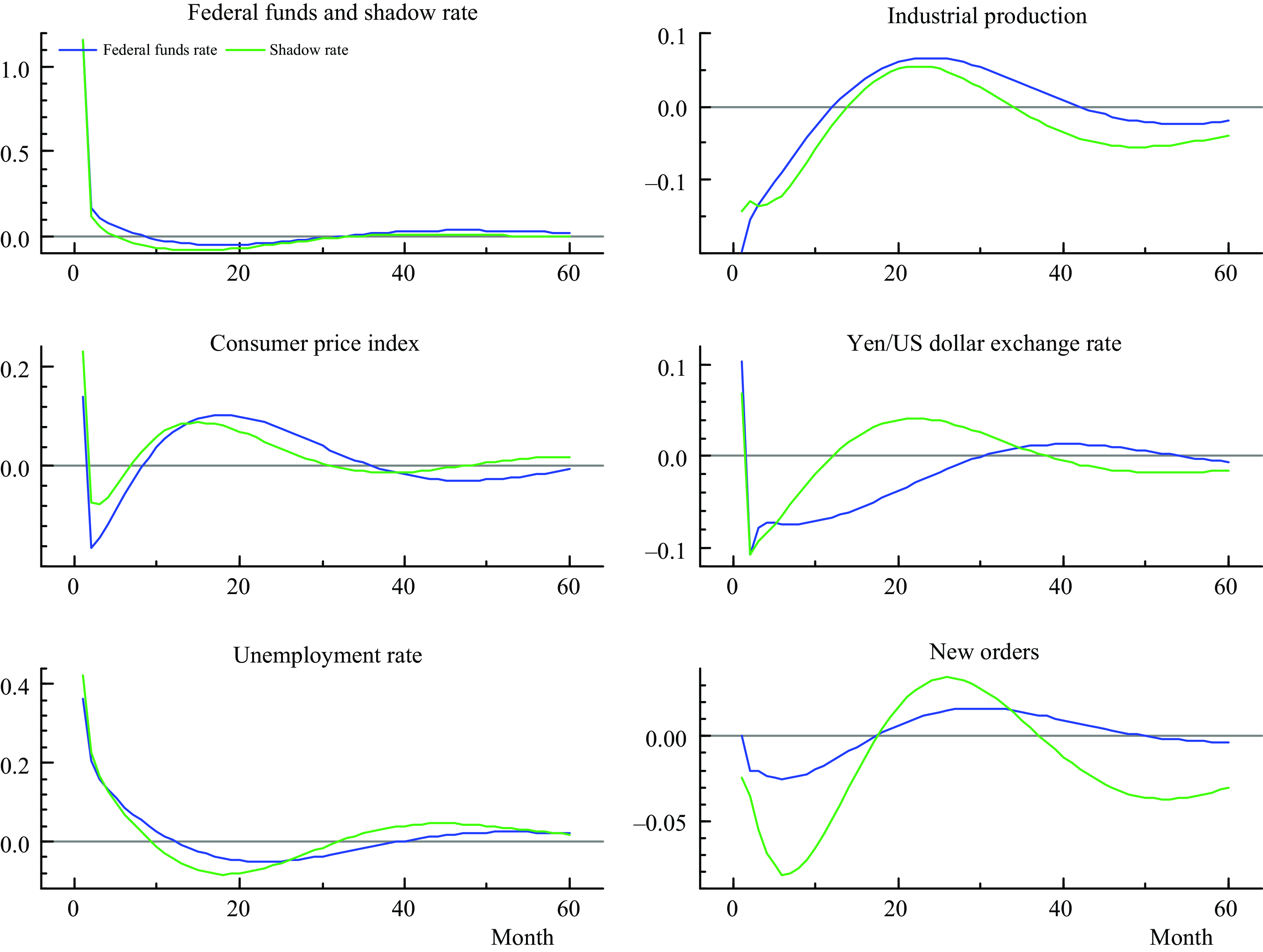
Figure 7. Impulse responses from a contractionary monetary policy shock.
Overall, the impulse responses are similar between the effective and shadow rates exhibiting hump-shaped reactions from the score-driven FAQVAR model. As we can see on the top left response, the shadow rate is even further negative in comparison to the FFR, as a result the initial impact for industrial production is relatively moderate. The consumer price index response still shows a price puzzle (positive reaction after a contractionary shock) in the first month, for then generate a disinflationary effect, and a lower increase in the medium term when considering the shadow rate. Also, the unemployment rate and new orders generate slightly bigger reactions from the shadow rate shock, and there is a more pronounced hump-shaped reaction in the exchange rate response.
6. Conclusions
This research studies a FAQVAR model, which allows the assessment of macroeconomic policies in turbulent times. The benefit of this approach is its flexibility as a nonlinear model and its robustness to critical episodes such as the U.S. financial crisis and the pandemic, when I evaluate the U.S. monetary policy since 1959. Unlike traditional FAVARMA models, FAQVAR models assume a Student t distribution model for their multivariate errors capable of accommodating big shocks, and they are observation and score-driven. The addition of these features generates stable estimates through turbulent episodes from FAQVAR models that are not well captured in the FAVARMA specification. In addition, the estimates from the proposed model are robust to the number of factors, pre-pandemic sample, and ZLB times.
As compared to the base FAVARMA model, the FAQVAR model generates a better in-sample fit and the generated impulse responses are hump-shaped. An assessment of monetary policy in the USA unveils that the characterized Student t errors provide a significant improvement to macro-modeling relative to FAVARMA models and the impulse responses from factors and monetary shocks are robust. Further, the impulse responses to a group of informational variables are in line with economic theory.
The proposed model allows several extensions, which include the modeling of heteroskedastic errors, time-varying parameters for the multivariate location model, specific modeling at or around the lower bound with interactive or Markov-switching models, and additional identifications for structural shocks.
Supplementary material
The supplementary material for this article can be found at https://doi.org/10.1017/S1365100523000330


 Open access