


1 Introduction
For decades judgment analysts have successfully used multiple regression to model the organizing cognitive principles underlying many types of judgments in a variety of contexts (see Brehmer & Brehmer, Reference Brehmer, Brehmer, Brehmer and Joyce1988; Cooksey, Reference Cooksey1996; Dhami, et al., Reference Dhami, Hertwig and Hoffrage2004, for reviews). Most often these models depict the individual judge or decision maker as combining multiple differentially weighted pieces of information (cues) in a compensatory manner to arrive at a judgment. Further, these analyses portray those who have acquired expertise on a judgment task as applying their judgment model or “policy” with regular, although less than perfect, consistency. The ability of linear regression models to accurately reproduce such expert judgments under various conditions has been discussed in detail (e.g., Dawes, Reference Dawes1979; Dawes & Corrigan, Reference Dawes and Corrigan1974; Einhorn & Hogarth, Reference Einhorn and Hogarth1975). If one accepts the proposition that people’s judgments can be modeled as though they are multiple regression equations, questions arise such as: 1) How many of the available cues does the individual use? and 2) How should the number of cues used be determined?
Too many researchers blindly apply statistical significance tests to inform them - in a kind of deterministic manner - whether judges did or did not attend to specific cues. If the t-test calculated on a cue’s weight is significant, then the cue is counted as being attended to by the judge. Relying on p values in this way is a problem because these values are affected by the number of cues and number of cases presented to the judge during the task and by how well the overall regression equation fits the total set of responses.
This issue is discussed in this note which is organized as follows: First, examples from the judgment literature are reviewed to illustrate the existence of the problem. Second, notation commonly used by judgment analysts when describing regression procedures is introduced. Third, using this notation, a method for calculating the post-hoc power of t-tests on regression coefficients based on the noncentral t distribution is described. Fourth, this method is applied to estimate the number of cases necessary for statistical significance in order to illustrate how the investigator’s conclusions about the number of cues attended to in a judgment task should be informed by considerations of type II error. Finally, an SPSS program for performing the calculations is described and provided in the Appendix.
2 Some examples in the judgment literature
Although it is reasonable to conclude that a “significant” cue is important to the judge and reliably used as he or she makes judgments, the converse does not follow. When a cue’s weight (regression coefficient, standardized regression coefficient, or squared semipartial correlation) is not significant, it does not necessarily mean that the cue is unimportant; there may simply be insufficient statistical power to produce a significant test result. Determining the number of cues to which an individual attends is an important issue from both practical and theoretical viewpoints. In a practical sense, informing poorly performing judges that they should attend to more (or different) cues than they apparently do can improve their accuracy (see Balzer, et al., Reference Balzer, Doherty and O’Connor1989, for review of cognitive feedback). Theories of cognitive functioning have long considered determining the amount of information we process to be a relevant question (e.g., Gigerenzer & Goldstein, Reference Gigerenzer and Goldstein1996; Hammond, Reference Hammond and Hammond1966; Miller Reference Miller1956).
In the typical judgment analysis the problem of type II error is overlooked. I know of no studies in the judgment analysis literature that report the power of the significance tests on cue weights when these tests are relied upon to determine the number of cues being used by a judge. While an exhaustive review of the empirical literature is beyond the scope of this note, a few examples are presented to illustrate the problem.
Phelps and Shanteau’s (Reference Phelps and Shanteau1978) purportedly determined the number of cues used by expert livestock judges in making decisions using two different experimental (“controlled” and “naturalistic”) designs. The same seven livestock judges rated the breeding quality of gilts (female breeding pigs) in two completely within-subject experiments. The controlled design used a partial factorial design in which each judge made 128 judgments of gilts described on 11 orthogonal cues. The naturalistic design used eight photographs of gilts. In this experiment the judges first rated the breeding quality of the gilt in each photo and then rated each photo on the same 11 cues used in controlled design. This procedure was repeated, resulting in a total of 16 judgments per judge. The authors then used significance tests to determine whether specific cues were being used by each judge in the two experiments. An important finding was that the judges used far more cues (mean = 10.1) in the controlled design than they did in the naturalistic design (mean = 0.9). The relevant data are summarized in Table 1. Using the F statistics reported in their Tables 1 and 2 to calculate estimates of effect sizes (η2) reveals some paradoxical results; many of the cues showed stronger relationships to judgments in the naturalistic design. Because of the lower statistical power in the naturalistic design (the controlled design presented 128 cases whereas the naturalistic design presented only 16) fewer cues were counted as significant and it was concluded that less information was being used by all judges under the naturalistic design.
Table 1: Summary of results from Phelps and Shanteau (1978) with addition of effect size estimates.

Table 2: Illustration of the influence of the number of cases m* on t-tests of regression coefficient

Note: The regression coefficient b = -0.423 and SEb = 0.386 for m = 30. The t-test of this coefficient was t = -1.096, p = .284; post-hoc power of the ttest is given by the Eq. (3) as .182. Due to negative sign of regression coefficient, resulting t-test values are negative; the sign has been omitted for clarity of presentation.
When comparing the results of the two experiments the authors attributed the difference in the amount of information used by the experts to the stimulus configuration, “...the source of the discrepancy seems to be in the intercorrelations among the characteristics and not in the statistical analysis” (Phelps & Shanteau, Reference Phelps and Shanteau1978, p.218). Although Phelps and Shanteau pointed out that the F statistics they report could easily be expressed as estimates of effect size they did not do so. If they had, they may have come to a different conclusion about the influences of naturalistic and controlled cue configurations in their judgment tasks.
One area of research particularly sensitive to the problem at hand is the study of self-insight into decisions. The assessment of self-insight in social judgment studies has traditionally compared statistical weights (derived via regression equations) with subjective weights. A widely accepted finding is that people have relatively poor insight into their judgment policies (see Brehmer & Brehmer, Reference Brehmer, Brehmer, Brehmer and Joyce1988; Harries, et al., Reference Harries, Evans and Dennis2000; Slovic & Lichtenstein, Reference Slovic and Lichtenstein1971, for reviews). In most studies assessing insight, judges are required to produce subjective weights (e.g., distributing 100 points among the cues). “It was the comparison of statistical and subjective weights that produced the greatest evidence for the general lack of self-insight” (Reilly, Reference Reilly1996, p. 214). Another robust finding from this literature is that people report using more cues than are revealed by regression models. “A cue is considered used if its standardized regression coefficient is significant” (Harries, et al., Reference Harries, Evans and Dennis2000, p. 461).
Two influential studies on insight by Reilly and Doherty (Reference Reilly and Doherty1989, Reference Reilly and Doherty1992) asked student judges to recognize their judgment policies among those from several other judges. In the first study seven of eleven judges were able to identify their own policies. In contrasting this finding to previous studies the authors noted “These data reflect an astonishing degree of insight” (Reilly & Doherty, Reference Reilly and Doherty1989, p. 125). In the second study the number of cues and the stimulus configuration were manipulated. Overall, 35 of 77 judges were able to identify their own policies. The authors reconciled this encouraging finding with the prevailing literature on methodologic grounds, arguing that the lack of insight shown in previous studies might be related to people’s inability to articulate their policies. “There is the distinct possibility that while people have reasonable self-insight on judgment tasks, they do not know how to express that insight. Or pointing the finger the other way round, while people do have insight we do not know how to measure it” (1992, p. 305).
In both these studies, when judges were presented with policies, each judge’s set of cue weights (squared semipartial correlations in this case) was rescaled to sum to 100, and importantly, cues which did not account for significant (p < .01) variance were represented as zeros. The authors noted the majority of judges (in both studies) indicated that they had relied on the presence or absence of zeros as part of the search strategy used to recognize their own policies. The use of significance tests to assign specific cues a rescaled value of zero in these studies is problematic for two reasons. First, the power of a significance test on a squared semipartial correlation in multiple regression is affected by the value of the multiple R2. As R2 increases, smaller weights are more likely to be significant. Second, the power of these significance tests is affected by the number of predictors in the regression equation. The net result was that the criterion used to assign zero to a specific cue was not constant across judges. Only when all judges are presented with the same number of cues and all have equal values of R2 for their resultant policy equations could the criterion be consistently applied.
To illustrate, Reilly and Doherty (Reference Reilly and Doherty1989) presented 160 cases containing 19 cues to each judge. Consider two judges with different values of R2 based on 18 of the cues, say .90 and .50. The minimum detectable effect (i.e., smallest weight that the 19th cue could take and still be significant) for the first judge is .008 but .039 for the second judge. The same problem exists in the 1992 study that used 100 cases and is compounded by the fact that the authors manipulated the number of cues presented to the judges; half the sample rated cases described by six cues and the other half rated cases described by twelve cues. In the recognition portion of both studies the useful pattern of zeros in the cue profiles was an artifact introduced arbitrarily by the use of significance tests. Had the authors used p < .05 rather than p < .01 to assign zeros, their conclusions about insight might have been astonishingly different.
Harries et al. (Reference Harries, Evans and Dennis2000, Study 1), examining the prescription decisions of a sample of 32 physicians, replicated the finding that people are able to select (recognize) their policies among those from several others. This study followed up on the participants in a decision making task (Evans, et al., Reference Evans, Harries, Dennis and Dean1995) in which 100 cases constructed from 13 cues were judged and regression analysis was used to derive decision policies. Judges also provided subjective cue weights, first indicating the direction (sign) of influence, then rating how much (0–10 scale) the cue had bearing on their decisions. When comparing tacit to stated policies (i.e., regression weights to subjective weights) Harries et al. (Reference Harries, Evans and Dennis2000) described a “triangular pattern of self-insight”: a) cues that had significant weights were the ones that the judge indicated he or she used, b) where the judge indicated that a cue was not important it did not have a significant weight, and c) there were cues that the judge indicated were important but which did not have significant weights. The authors’ choice of p value for determining whether a cue was attended to in the tacit policies had influence on all three sides of this triangular pattern.
Approximately 10 months following the decision-making task, participants were presented with sets of decision policies in the form of bar charts rather than tables of numbers. Cues with statistically significant weights were presented as darker bars. With only four cues having significant effects on decisions (Harries et al., Reference Harries, Evans and Dennis2000, p. 457), it is possible that physicians used the presence or absence of lighter bars in the same way that Reilly and Doherty’s students made use of zeros in their recognition strategies. Had more cues been classified and presented as significant, the policy recognition task might have proved more difficult.
Other examples exist in the applied medical judgment literature. Gillis et al. (Reference Gillis, Lipkin and Moran1981) relied extensively on p values of beta weights for describing the judgment policies of 26 psychiatrists making decisions to prescribe haloperidol based on 8 symptoms (see their Table 4). Averaged across judges, the number of cues used was 2.4, 1.9, or 1.0 depending on the p value employed (.05, .01, or .001, respectively). Had the investigators chosen to compare the number of cues used with self-reported usage, which of the three p values ought they have relied upon? Had the investigators rescaled and presented policies to participants for recognition (via Reilly & Doherty), their choice of p value could have affected the difficulty of the recognition task.
More recently, in a judgment analysis of 20 prescribing decisions made by 40 physicians and four medical guideline experts, Smith et al. (Reference Smith, Gilhooly and Walker2003) reported “The number of significant cues ... varied between doctors, ranging from 0 to 5” (p. 57), and among the experts “The mean number of significant cues was 1.25” (p. 58). It is noteworthy that this study presented doctors with a relatively small number of cases thus leaving open the meaning of “significant.” Had Smith et al. presented more than 20 cases, they may have concluded (based on p values) that doctors and guideline experts attended to more information when making prescribing decisions.
Other models of judgment, known as “fast and frugal heuristics” have recently been proposed as alternatives to regression models (see Gigerenzer, Reference Gigerenzer, Koehler and Harvey2004; Gigerenzer & Kurzenhäuser, Reference Gigerenzer, Kurzenhäuser, Bibace, Laird, Noller and Valsiner2005; Gigerenzer, et al., Reference Gigerenzer and Todd1999). A hallmark of fast and frugal models is that they are purported to rely on far fewer cues than do judgment models described by regression procedures. When comparing these classes of models, the number of cues the judge uses is one way of differentiating the psychological plausibility of these models (see Gigerenzer, Reference Gigerenzer, Koehler and Harvey2004). Studies comparing regression models with fast and frugal models have implied that significance testing is the method of determining the number of cues used despite the fact that the developers of these methods (e.g., Stewart, Reference Stewart, Brehmer and Joyce1988) made no such claim and currently advise against it (Stewart, personal communication, July 2, 2007).
In a study comparing regression with fast and frugal heuristics, Dhami and Harries (Reference Dhami and Harries2001) fitted both types of models to 100 decisions made by medical practitioners. They report that number of cues attended to was significantly greater when modeled by regression than by the matching heuristic. According to the regression models the average number of cues used was 3.13 and the average for the fast and frugal models was 1.22. “In the regression model a cue was classified as being used if its Wald statistic was significant (p < .05) ...” (Dhami & Harries, Reference Dhami and Harries2001, p. 19). In the heuristic model, the number of cues used was determined by the percentage of cases correctly predicted by the model; significance tests were not used. At issue is not the fact that different criteria were used to count the cues used under the two types of models (although this is a problem when evaluating their results), but rather, that the authors relied on a significance test known for some time to be dubiousFootnote 1, and their choice of p value for counting cues may have biased their data to favor the psychological plausibility of the fast and frugal model. Had they used p < .01 rather than p < .05, the average number of cues used according to the regression procedure would presumably have been lower, and perhaps not different than the average found for the matching heuristic.
In the last few paragraphs, examples from the literature have been presented that highlight the problems associated with using significance tests to determine the number of cues used in judgment tasks. Tests of significance on regression coefficients or R2 are really not very enlightening for distinguishing the “best” judgment model from among a set of competing models. The true test of which model (among a set of contenders) is the best is the ability of the equation to predict the judgments made in some future sample of cases, the data from which were not used to estimate the regression equation. The remaining sections of this note formally present the regression model as used in judgment analysis and discuss a method for assessing the power of significance tests so as to provide more information to judgment analysts who use them.Footnote 2
3 Notation
Following Cooksey (1996), let the k cues be denoted by subscripted X’s (e.g., X1 to Xk). In a given judgment analysis a series of m profiles or cases is constructed where each case is comprised of k cues. The judge or subject makes m responses Ys to these cases. The resulting multiple regression equation representing the subject’s judgment policy is of the general form
where b 0 represents the regression constant and the remaining b i represent regression coefficients for each cue where each coefficient indicates the amount by which the prediction of Ys would change if its associated cue value changed by one unit while holding all other cue values constant, and e represents residual or unmodeled influences.
Tests of significance may be employed to assess the null hypothesis that the value of bi in the population is zero, thus H 0: bi = 0 against the alternative H 1: bi ≠ 0. The ratio b i / SEb i is distributed as a t statistic with degrees of freedom (df) = m - k - 1. The SEbi is found as

where sdYs and sdXi are, respectively, the standard deviations for the judgments and for the ith cue’s values; ![]() is the squared multiple correlation for the judgment equation; and
is the squared multiple correlation for the judgment equation; and ![]() is the squared multiple correlation from a regression analysis predicting the ith cue’s values from the values of the remaining k − 1 cues. In standard multiple regression it can be shown that the significance test of bi (t = bi / SEbi) is equivalent to testing significance of the standardized regression coefficient βi and the squared semipartial correlation associated with Xi (see Pedhazur, Reference Pedhazur1997). This is fortunate because most commercially available statistics packages routinely print values for SEbi but not for SEβi.Footnote 3
is the squared multiple correlation from a regression analysis predicting the ith cue’s values from the values of the remaining k − 1 cues. In standard multiple regression it can be shown that the significance test of bi (t = bi / SEbi) is equivalent to testing significance of the standardized regression coefficient βi and the squared semipartial correlation associated with Xi (see Pedhazur, Reference Pedhazur1997). This is fortunate because most commercially available statistics packages routinely print values for SEbi but not for SEβi.Footnote 3
4 Post-hoc power analysis on t-test of regression coefficients
Having analyzed data from a judgment analysis using multiple regression it is rather simple to calculate the statistical power associated with the t-test of each regression coefficient. All that is needed from the analysis is the observed value of t, its df, and the a priori specified value of α. To obtain the power of the t-test that H 0: bi = 0 for α = .05, one may employ the noncentral distribution of the t statistic (see Winer et al., Reference Winer, Brown and Michels1991, pp. 863–865), here denoted ![]() , which is actually a family of distributions defined by df and a noncentrality parameter δ, hence
, which is actually a family of distributions defined by df and a noncentrality parameter δ, hence ![]() (df; δ). In the present context δ = bi / SEbi. The power of the t-test on the regression coefficient may then be determined as
(df; δ). In the present context δ = bi / SEbi. The power of the t-test on the regression coefficient may then be determined as
Thus the probability that the noncentral t ′ will be greater than the critical value of t, given the observed value of t = b i / SEb i, is equal to the power of the test that H 0: b i = 0 for α = .05. For example, consider the following result from an illustrative judgment analysis involving k = 6 cues and m = 30 cases provided by Cooksey (Reference Cooksey1996, p.175). The unstandardized regression coefficient for a particular cue is b = 0.267, (β = .295) its standard error is 0.146, thus t = 0.267/0.146 = 1.829. The critical value for t with df = 30 - 6 - 1 = 23, and α = .05 for a two-tailed test is 2.069; consequently the null hypothesis is not rejected and it might be concluded that this cue is unimportant to the judge. Using the information from this significance test and the noncentral distribution of t ′(df = 23; δ = 1.829) we find that the probability of type II error = .582, and thus the power to reject the null is only .418. To claim that this cue is “unimportant to the judge,” or “is not being attended to by the judge” does not seem justifiable in light of the rather high probability of type II error.
5 Estimating the number of cases necessary for significant t-test of regression coefficients
Faced with such a nonsignificant result, as in the example presented above, the judgment analyst may wish to know the extent to which this outcome was related to the study design. In particular, how was the nonsignificant t-test of the cue weight affected by his or her decision to present m cases to the judge instead of some larger number m*? To address this question we must first clarify the types of the stimuli used in judgment studies.
Brunswik (Reference Brunswik1955) argued for preserving the substantive properties (content) of the environment to which the investigator wishes to generalize in the stimuli presented during the experimental task. Hammond (Reference Hammond and Hammond1966), in attempting to overcome the difficulties inherent in such representative designs, distinguished between “substantive” and “formal” sampling of stimuli. Formal stimulus sampling concerns the relationships among environmental stimuli (with content ignored). The following discussion is limited to studies employing formal stimulus sampling. When taking the formal approach to stimulus sampling, the investigator’s focus is on maintaining the statistical characteristics of the task environment (e.g., k, sdXi and R 2Xi) in the sample of stimuli presented to the participant. These characteristics of the environment may be summarized as a covariance matrix, Σ. If the investigator obtains a sample of m stimuli from the environment, the covariance matrix Sm, may be computed from the sample and compared with Σ. The basic assumption of formal stimulus sampling may then be stated as Sm ≈ Σ. Whether probability or nonprobability sampling is used, it is possible for the investigator to construct an alternative set of m * cases such that Sm* = Sm. Under the condition that Sm* = Sm ≈ Σ, it is possible to estimate SEb i*, the standard error of the regression coefficient based on the larger sample of cases m *. Inspection of Eq. (2) reveals that SEb i becomes smaller as the number of cases m becomes larger. Holding all other terms in Eq. (2) constant, SEb i* may be found as

Substituting SEb i* in place of SEb i when calculating t-test on b i allows us to estimate the impact of increasing m to m * on type I error in the same judgment analysis. Making the same substitution in Eq. (3) allows us to estimate the impact of this change on type II error and power.
Stewart (Reference Stewart, Brehmer and Joyce1988) has discussed the relationships among k, R2Xi, and m and recommends m = 50 as a minimum for reliable estimates of cue weights when k ranges from 4 - 10 and R2Xi=0. He points out that as the intercorrelations among the cues increases the number of cases will need to be increased in order to maintain reasonably small values of SEbi. Of course the investigator’s choice of m should also influenced by his or her sense of subject burden. Stewart notes from empirical evidence that most judges can deal with making between “40 to 75 judgments in an hour, but the number varies with the judge and the task” (Stewart, Reference Stewart, Brehmer and Joyce1988, p.46). In discussing the design of judgment analysis studies Cooksey (Reference Cooksey1996) has suggested that the optimal number of cases may be closer to 80 or 90. Reilly and Doherty (Reference Reilly and Doherty1992) reported the average time for 77 judges to complete 100 12-cue cases was 1.25 hours. In a recent study by Beckstead and Stamp (Reference Beckstead and Stamp2007) 15 judges took on average 32 minutes (range 20–47) to respond to 80 cases constructed from 8 cues.
For the example given in the previous section, if the investigator had used m* = 40, rather than m = 30, Eq. (4) indicates that SEbi* would have been 0.122 and the resulting value for the t-test would have been 2.191 with p = .036. The point here is that had the investigator presented 10 more cases (sampled from the same population), he or she might have come to a different conclusion about the number of cues attended to by this judge.
6 An SPSS program for calculating post-hoc power in regression analysis
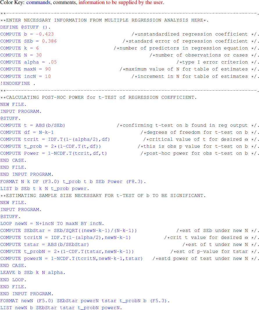
The calculations for determining post-hoc power for tests of regression coefficients as used in judgment analysis studies and estimating SEb i* are straightforward and based on statistical theory, however detailed tables of noncentral t distributions are hard to come by. The author has written an SPSS program for performing these calculations that is provided in the Appendix. To illustrate the program, consider another cue taken from the same example found in Cooksey (Reference Cooksey1996, p.175) where b = -0.423, SEb = 0.386, and k = 6 for m = 30. Inserting these values into the program and specifying that the number of cases increase to 90 by increments of 10, produces the result shown in Table 2.
As m * increases, the estimated values of SEb * decrease and the values of the t-statistic increase. According to these estimates, the t-test on this cue would have been significant had approximately 85 cases been used in the judgment task. The program can be “rerun” specifying a smaller increment in order to refine this estimate. The results provided by such an analysis could also be very useful in the planning of subsequent judgment studies.
7 Summary and recommendations
In this note the issue of type II error has been raised in the context of determining whether or not a cue is important to a judge in judgment analysis studies. Some of the potential pitfalls of relying on significance tests to determine cue utilization have been pointed out and a simple method for calculating post-hoc power of such tests has been presented. A short computer program has been provided to facilitate these analyses and encourage the calculation (and reporting) of statistical power when judgment analysts rely on significance tests to inform them as to the number of cues attended to in judgment tasks.
As a tool for understanding the individual’s cognitive functioning, regression analysis has proved to be quite useful to judgment researchers for over 40 years. In this role I believe that its true value lies in its descriptive, not its inferential, facility. Like any good tool, if we are to continue our reliance upon it we must insure that it is in proper working order and not misuse it.
There are alternative models of judgment being advocated (e.g., probabilistic models proposed by Gigerenzer and colleagues) that do not fall prey to the problems associated with regression analysis. However, as judgment researchers develop, test, and apply these models, questions about the amount of information (i.e., the number of cues) individuals use when forming judgments and making decisions are bound to arise. The strongest evidence for the veracity of any judgment model is its ability to predict the outcomes of future decisions.
The practice of post-hoc power calculations as an aid in the interpretation of nonsignificant experimental results is not without its critics (e.g., Hoenig & Heisey, Reference Hoenig and Heisey2001; Nakagawa & Foster, Reference Nakagawa. and Foster2004). Hypothesis testing is easily misunderstood but when applied with good judgment it can be an effective aid to the interpretation of experimental data (Nickerson, Reference Nickerson2000). Higher observed power does not imply stronger evidence for a null hypothesis that is not rejected (see Hoenig & Heisey, Reference Hoenig and Heisey2001 for discussion of the power approach paradox). Some researchers have argued for abandoning the use hypothesis testing altogether and relying instead on the confidence interval estimation approach (Armstrong, Reference Armstrong2007; Rozeboom, Reference Rozeboom1960). I tend to agree with Gigerenzer and colleagues who put it succinctly, “As long as decisions based on conventional levels of significance are given top priority ... theoretical conclusions based on significance or nonsignificance remain unsatisfactory without knowledge about power” (Sedlmeier & Gigerenzer, Reference Sedlmeier and Gigerenzer1989, p. 315).
Appendix
The following is an SPSS program to calculate post-hoc power of t-test on regression coefficients and to estimate sample size needed for significance of such tests. After typing the commands into a syntax window and supplying information specific to your analysis, simply run the program to obtain results similar to those found in Table 2.


 Open access