


I. Introduction
An important concept underlying wine production and appreciation in the Old World (France, Germany, Italy, and Spain) is terroir, which refers to the characteristics of a location that impart special qualities to the wine produced (Gergaud and Ginsburgh, Reference Gergaud and Ginsburgh2010). In France, the Appellation d'Origine Contrôlée (AOC) system—and similar systems adopted in other major wine-producing countries—is based on the geographic location of grape production and is thereby predicated on this notion of terroir. A considerably more recent U.S. system of American Viticultural Areas (AVAs) likewise reflects the location of grape production. Finer geographical designations are known as Sub-AVAs.
These AVA and Sub-AVA designations allow wineries to identify the origin of the grapes used in producing their wines, but what is the real value of terroir in this American context? Does the “reality of terroir”—the location-specific geology and geography (including climate)—predominate in determining the quality of wine, as is assumed to be the case in Europe? And/or does the “concept of terroir”—the location within an officially named appellation—impart reputational value to grapes and the wine they yield? Does the location within an appellation impart additional value to vineyards?
To address these questions, and thereby the fundamental question of the role of terroir in New-World wine production, we examine whether observable site attributes—slope, aspect, elevation, and climate—or appellation designations are more important determinants of vineyard prices in the most important wine-producing region in the United States: Napa and Sonoma Counties in California. We carry out this examination with a hedonic price analysis of vineyard sales.Footnote 1 By focusing on vineyard sale prices rather than wine (bottle) prices, we can directly examine the price effects of terroir and avoid confounding influences of nonvineyard inputs into wine production, including the skills and techniques of the winemaker.
It is conceivable that site attributes, AVA designations, or both influence vineyard prices. At one extreme, if site attributes affect wine quality and consumers are able to discriminate such quality, then vineyard prices would depend on site attributes alone,Footnote 2 because AVA designations would simply be redundant.
At the other extreme, site attributes might be irrelevant, with vineyard prices being fully explained by AVA designations. In this case, the implication is that terroir matters economically as a concept but perhaps not as a fundamental biophysical reality. There might be three possible explanations for this. First, if producers believe that consumers will pay more for wines from more-prestigious designations, then they might be more willing to pay for vineyard properties in those areas.Footnote 3 In this case, any appreciation that consumers might express for an area's terroir would be founded on reputation rather than reality.Footnote 4 Second, if buyers are less informed than sellers about vineyard attributes and how they affect wine quality, then buyers might use AVA designations as signals of quality. Third, producers might bid up the value of vineyards located in designated appellations because of the personal prestige associated with owning these properties.
An intermediate case lies between these two extremes of, on the one hand, the biophysically dominant reality of terroir (and the consequent redundancy of AVA designations) and, on the other hand, terroir’s mattering not as a fundamental reality but only as a concept economically (and the consequent insignificance of site attributes in explaining vineyard prices). In the intermediate case, consumers might be able to discriminate imperfectly among wines and might therefore use AVA designations as signals of the average quality of wines from respective areas, or they might derive utility directly from drinking wines that they know to be of particular pedigrees. In this intermediate case, site attributes and AVA designations would influence vineyard prices, with estimated coefficients for site attributes measuring how producers valued intra-AVA differences in vineyard characteristics. In other words, producers would attach premiums to site attributes that enhanced wine quality if consumers could perceive and were willing to pay for quality differences.
By executing a hedonic analysis of the factors affecting vineyard sales prices in Napa and Sonoma Sub-AVAs,Footnote 5 we distinguish among these three cases and thereby assess the value of terroir in the California context. In our previous analysis of vineyard sales in Oregon's Willamette Valley, we found that AVA designations but not site attributes were significant, meaning that terroir mattered economically but not biophysically. In the case of California's premier wine-production regions, we find a more nuanced result in which AVA designations and location attributes significantly affect vineyard sale prices, supporting the intermediate case in which terroir is validated as a conceptual and as a fundamental reality.
In Section II, we briefly review previous, related literature and highlight the differences between this analysis and our previous work in Oregon. In Section III, we describe our analytical approach, including our treatment of potential sample-selection bias. In Section IV, we describe our empirical results. Finally, we conclude in Section V.
II. Previous Literature
The analysis we document in this paper builds on our previous work and that of others,Footnote 6 including Gergaud and Ginsburgh (Reference Gergaud and Ginsburgh2010). We build on their work by examining the effects of appellation designations in addition to the effects of site characteristics. By using GIS-based information to develop detailed physiographic profiles of parcels, we are able to measure site characteristics more precisely than have most previous researchers. Earlier studies using fine-scale data include Ashenfelter and Storchmann's (Reference Ashenfelter and Storchmann2010) investigation of the effects of climate on vineyards in the Mosel Valley and the analysis by Gergaud, Plantinga, and Ringeval-Deluze (Reference Gergaud, Plantinga and Ringeval-Deluze2017) of the price effects of obsolete vineyard ratings in the Champagne region.
Our analysis also differs from most previous work by employing vineyard sale prices as the dependent variable instead of wine (bottle) prices or ratings (Ashenfelter and Storchmann, Reference Ashenfelter and Storchmann2010; Castriota and Delmastro, Reference Castriota and Delmastro2015; Costanigro, McCluskey, and Goemans, Reference Costanigro, McCluskey and Goemans2015; Gergaud and Ginsburgh, Reference Gergaud and Ginsburgh2010). In our investigation into the value of terroir, this difference avoids the potentially confounding influences of nonvineyard inputs into wine production (such as winemaking techniques) and reputational effects of producers and regions. Costanigro, McCluskey, and Goemans (Reference Costanigro, McCluskey and Goemans2015) find evidence of reputation premia attached to wine bottle prices after controlling for quality scores from blind tastings by experts.
Although the overall purpose of our analysis—assessing the value of terroir in a New-World context—is similar to our previous work (Cross, Plantinga, and Stavins, Reference Cross, Plantinga and Stavins2011a, Reference Cross, Plantinga and Stavins2011b), this study departs from and significantly improves on that work in several ways. First, our current measurement of vineyard attributes is much more precise. In our previous work, we measured those attributes as average values across entire parcels, but here we geographically locate each vineyard within the sold property and measure its specific local attributes. Second, we control for the effects of varietals on vineyard prices. For our previous study of the Willamette Valley of Oregon, we lacked information on varietals, although we knew that Pinot Noir accounted for about three-quarters of vineyard acreage in that region. Third, we now examine the effects of climate, as meaningful climatic variations exist within the geographic Napa-Sonoma region. Fourth, because we have information about vineyard sales outside any AVA or Sub-AVA, we can estimate the contribution of Sub-AVAs to vineyard prices. Fifth, as we explain below, we suspect that the sample of sold parcels may not be representative of the population of vineyard parcels in the Napa-Sonoma region. We therefore locate and measure attributes of the universe of vineyards—sold or not—in Napa and Sonoma Counties and adjust the results for potential sample-selection bias.
III. Analytical Approach
We investigate the relationship between vineyard sales prices, site attributes, and appellation designations with extensive data on vineyard sales in Napa and Sonoma Counties for the years 1991 through 2007. With a hedonic model of vineyard sales prices, we can identify the degree to which sales prices were associated with site attributes and appellation designations and thereby can assess the degree to which terroir functions as a concept, a reality, or both.
The hedonic price model is a reduced-form equilibrium model and thus captures demand and supply factors. In our application, we expect prices to be determined primarily by the demand for grapes and for the wine produced from those grapes. Given that we analyze properties with existing vineyards, any fixed costs of vineyard establishment are sunk and will not be reflected in market prices. Grape production also involves variable costs for vineyard management and harvest. However, with the possible exception of steeply sloped parcels, we would expect little variation in variable costs among vineyards in our sample.
In a competitive market, the price of a vineyard equals the present discounted value of the anticipated stream of rents generated by the land. These rents may vary in the future with changes in climate, technology, and other factors that make a given vineyard parcel more or less productive. Although we do not explicitly model the future rent stream, the site attributes in our model capture, to some degree, expectations of future rent changes. For example, if higher elevations are expected to become better suited for grape production under future climate changes, this trait should raise the current value of higher-elevation sites and be reflected in the estimated elevation parameters. In fact, a recent study by Severen, Costello, and Deschenes (Reference Severen, Costello and Deschenes2016) finds evidence that climate-change forecasts are being reflected in current farmland prices.
A. Dependent Variable for Hedonic Estimation: Vineyard Value
The dependent variable in our hedonic model is the natural log of real vineyard price per acre, denoted as lnP. Many sales include nonvineyard assets, such as buildings and additional, nonvineyard land. So, to obtain the price of vineyards, we subtract from total sales price the appraiser-based estimate of the value of nonvineyard assets (buildings, building sites, plantable and residual land, and winery permits). Then, by dividing the vineyard price by the vineyard area and expressing the result in constant (2007) dollars using the Consumer Price Index, we construct our dependent variable.
B. Independent Variables for Hedonic Estimation
Key independent variables include measures of vineyard area; indicator variables for AVAs and Sub-AVAs; shares of vineyards planted in various varietals; shares of vineyards in different aspect, elevation, and slope categories; and variables for local climate (Table 1). Soil characteristics are another potential determinant of vineyard prices. Based on an analysis described below, we control for soils using AVA dummy variables. We include vineyard area (A) and the square of this variable (A 2), because in our previous work in the Willamette Valley of Oregon, we found that the per-acre price declines as the parcel size increases, consistent with volume discounts offered by sellers.
Table 1 Variable Definitions and Summary Statistics

Indicator variables are included for 20 Sub-AVAs in which we observe vineyard sales. Three Sub-AVAs in Napa County (Chiles Valley, Stags Leap, and Wild Horse Valley) and three in Sonoma County (Carneros, Moon Mountain, Pine Mountain) are excluded due to lack of sales observations. A few properties are located in more than one Sub-AVA, and so we create separate categorical variables for these sales.Footnote 7 It is possible for vineyards to be within an AVA (Napa Valley, Russian River Valley, Sonoma Coast, or Sonoma Valley) but not within a Sub-AVA. When we include AVA dummies to control for soil characteristics, we cannot separately identify the effects of AVA designation. In total, we include 22 mutually exclusive indicator variables for Sub-AVAs. We compute the share of the vineyard planted in each of nine varietals: Cabernet Sauvignon, Chardonnay, Cabernet Franc, Merlot, Pinot Noir, Sauvignon Blanc, Syrah, Zinfandel, and other. If all vineyards are planted in the optimal varietal, conditional on site attributes, we do not expect the selected varietal to influence vineyard price. But if significant costs are associated with changing varietals, we may find price premiums associated with prized varietals, such as Cabernet Sauvignon. To estimate the price model, we omit the “other varietal” category.
We include variables for aspect, elevation, and slope of each vineyard, which are the key attributes—along with climate (see below)—that are often mentioned as indicators of terroir. We compute the share of the vineyard in each of nine aspect categories (south, southeast, southwest, etc.), including a category for “flat ground” and omitting the “west” category when the model is estimated. Elevation variables measure the share of the vineyard in each of seven categories (0 to 100 feet, 100 to 200 feet, etc.), with “600 to 700 feet” being the omitted category. Finally, we include variables for the share of each vineyard in six slope categories (1 to 2 degrees, 2 to 5 degrees, etc.), omitting the “0 to 1 degree” category.
We construct climate variables of temperature and precipitation using historical (1980 to 1989) weather data.Footnote 8 We compute the average difference between the daily high temperatures and daily low temperatures during the maturation and harvest period (July, August, and September).Footnote 9 Warm temperatures contribute to grape maturation, and daily temperature fluctuations are associated with acid and sugar development and flavor complexity (Robinson, Reference Robinson2006). We measure average precipitation over the entire growing season (February through September) as well as during the maturation and harvest period. Soil moisture levels as well as precipitation at bud break, fruit set, and harvest play important roles in vine health and fruit quality (Matthews and Anderson, Reference Matthews and Anderson1989).
Soil characteristics are a potentially important indicator of terroir. Gergaud et al. (Reference Gergaud, Plantinga and Ringeval-Deluze2017) find that vineyard prices in the Champagne region of France are significantly affected by the parcels’ limestone content. In contrast with our earlier work on the Willamette Valley of Oregon (Cross et al., Reference Cross, Plantinga and Stavins2011a), in which vineyards are found primarily on three or four soil types, vineyards in Napa and Sonoma Counties are found on sites with a much larger number of soil types. For the most disaggregated classification, 307 soil types are represented in our dataset (Natural Resource Conservation Service, 2016), making it infeasible to include variables for soil types in the hedonic price model.
A major concern with omitting soil variables from the hedonic model is that they may be correlated with the AVA and Sub-AVA designations, which could bias our parameter estimates.Footnote
10
However, because we observe the locations and characteristics of all (sold and unsold) vineyards in Napa and Sonoma Counties, we can use the entire dataset to investigate whether soils are a significant determinant of AVA and Sub-AVA designations. To this end, we estimate a series of index function models (one for each AVA or Sub-AVA) in which an unobserved index
 $y_j^\ast$
determines whether a given vineyard is included in the jth AVA or Sub-AVA. For each vineyard, we observe the binary outcome y
j
, where y
j
takes a value of 1 if the vineyard is part of the jth AVA or Sub-AVA, and is 0 otherwise. The outcome variable is assumed to be related to the index as follows: y
j
= 1 if
$y_j^\ast$
determines whether a given vineyard is included in the jth AVA or Sub-AVA. For each vineyard, we observe the binary outcome y
j
, where y
j
takes a value of 1 if the vineyard is part of the jth AVA or Sub-AVA, and is 0 otherwise. The outcome variable is assumed to be related to the index as follows: y
j
= 1 if
 $y_j^\ast \gt 0$
and y
j
= 0 if
$y_j^\ast \gt 0$
and y
j
= 0 if
 $y_j^\ast \le 0$
. Further, the index is expressed in terms of observable vineyard characteristics X and an unobserved disturbance term ε according to
$y_j^\ast \le 0$
. Further, the index is expressed in terms of observable vineyard characteristics X and an unobserved disturbance term ε according to
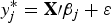 $y_j^\ast = {\bf X}{\prime}{\bf \beta} _j + \varepsilon $
, where
$y_j^\ast = {\bf X}{\prime}{\bf \beta} _j + \varepsilon $
, where
 ${\bf \beta} _j$
is a vector of parameters for the jth AVA or Sub-AVA.
${\bf \beta} _j$
is a vector of parameters for the jth AVA or Sub-AVA.
We estimate the
 ${\bf \beta} $
parameters using the linear probability model
${\bf \beta} $
parameters using the linear probability model
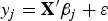 $y_j = {\bf X}^{\prime}{\bf \beta} _j + \varepsilon $
. With this model, we can more easily address spatial correlation in the errors than with a probit or logit specification. Because the AVAs and Sub-AVAs are geographically distinct areas, we might expect the errors to be correlated within AVAs or Sub-AVAs. We compute cluster-robust standard errors, where the clusters are defined as AVAs for the AVA models and Sub-AVAs for the Sub-AVA models. In all models, the independent variables include the varietal, aspect, elevation, and slope shares and the climate measures, as described above. We also include a set of variables for soil characteristics. We have four alternative sets of soil variables, which vary by degree of specificity: Each set includes 6, 24, 78, or 307 variables. We estimate a separate set of AVA and Sub-AVA models for each set of soil variables.
$y_j = {\bf X}^{\prime}{\bf \beta} _j + \varepsilon $
. With this model, we can more easily address spatial correlation in the errors than with a probit or logit specification. Because the AVAs and Sub-AVAs are geographically distinct areas, we might expect the errors to be correlated within AVAs or Sub-AVAs. We compute cluster-robust standard errors, where the clusters are defined as AVAs for the AVA models and Sub-AVAs for the Sub-AVA models. In all models, the independent variables include the varietal, aspect, elevation, and slope shares and the climate measures, as described above. We also include a set of variables for soil characteristics. We have four alternative sets of soil variables, which vary by degree of specificity: Each set includes 6, 24, 78, or 307 variables. We estimate a separate set of AVA and Sub-AVA models for each set of soil variables.
We find that soil characteristics are significant determinants of AVA designations, but not of Sub-AVA designations. Depending on which soil variables we use, between 2 and 21 percent of the estimated parameters on the soil variables are significantly different from zero in the AVA model sets. In contrast, at most 1 percent of the coefficient estimates for the soil variables are significant in Sub-AVA model sets. For the Sub-AVA models, the probability of Type II error is sufficiently low so that we can ignore the effects of soil at the Sub-AVA scale. However, the results for the AVA models suggest that we need AVA-level controls for soil. The most general approach is to include dummy variables for each of the AVAs, which is the approach we use. The dummy variable for the Northern Sonoma AVA is omitted for estimation.
C. Correcting Possible Sample-Selection Bias
In terms of land area, the vineyards sold between 1991 and 2007 represent only about 7 percent of all vineyard acreage in Napa and Sonoma, which suggests that our sample of sold vineyards may not be representative of the complete universe of vineyards. If a systematic basis determines which vineyards sell, failure to account for such selection in our sample would be a specification error that could produce inconsistent estimates (Heckman, Reference Heckman1979). To avoid this problem, we estimate the hedonic price model using Heckman's two-step estimation procedure. In the first step, we estimate a probit model in which the dependent variable is a binary indicator of whether a parcel sold, drawing on data for the universe of vineyards within Napa and Sonoma Counties. With these estimation results, we construct the inverse Mill's ratio, which is the ratio of the probability density function to the cumulative distribution function of the standard normal distribution (the probit model assumes that the error term follows a standard normal distribution). With Heckman's procedure, this ratio is included as a variable in the hedonic price equation estimated in the second step.
Heckman's two-step estimator can be unreliable in the absence of exclusion restrictions (Vella, Reference Vella1998). For our application, we identify two variables that can potentially explain whether a vineyard sells but that we expect to be uncorrelated with vineyard price. The first is the number of sold vineyards within a 2-kilometer buffer around a vineyard, excluding the vineyard itself (sale_count). If certain attributes of properties make them more likely to sell, and these attributes are spatially correlated, then the probability that a vineyard sells will increase in the count of nearby sales.Footnote 11
The other excluded variable is the share of the total parcel planted in vineyards (vineyard_share). Potential buyers can learn more about the value of nonvineyard land for grape production as the share of the parcel in vineyards increases. If buyers are seeking to expand the planted area, parcels with a larger vineyard share are more sought after and potentially more likely to sell. Better information about vineyard quality should raise the value of nonvineyard land but not affect the price of established vineyards.
These two variables are included in the first-stage probit model with those exogenous variables from the hedonic model that we can measure for unsold parcels. In addition, we include a set of year dummies in the hedonic model. Our data include sales in 1991 and the years 1993 to 2007. The dummy variable for 1991 is omitted for estimation.
D. Second-Stage Estimation of the Hedonic Price Function
After estimating the first-stage probit model and deriving from it the inverse Mills ratio, we specify the following hedonic price function and estimate its parameters:
 $$\eqalign{lnP_i\; & = \; \alpha + \; \beta _1\left( {A_i} \right) + \; \beta _2\left( {A_i^2} \right) + \mathop \sum \limits_{\,j = 1}^{26} \gamma _j\left( {AVA_{ij}} \right) + \mathop \sum \limits_{k = 1}^8 \delta _k\left( {V_{ik}} \right) + \mathop \sum \limits_{l = 1}^8 \zeta _l\left( {Asp_{il}} \right) \cr & \quad + \mathop \sum \limits_{n = 1}^6 \theta _n\left( {E_{in}} \right) + \mathop \sum \limits_{q = 1}^5 \kappa _q\left( {S_{iq}} \right) + \mathop \sum \limits_{r = 1}^3 \mu _r\left( {T_{ir}} \right) + \mathop \sum \limits_{s = 1}^2 \lambda _s\left( {R_{is}} \right) + \mathop \sum \limits_{t = 1}^{15} \pi _t\left( {Y_t} \right) \cr & \quad + \rho (M_i) + \; \varepsilon _{i,}}$$
where: P i = real vineyard sales price per acre for sale i (i = 1 to 188, as explained in text);
α = intercept;
A i = size of vineyard (acres);
AVA ij = AVA dummy variable or Sub-AVA designation j (where j = 1 to 26);
V ik = share of vineyard planted to varietal k (k = 1 to 8);
Asp il = share of vineyard located in aspect category l (l = 1 to 8);
E in = share of vineyard located in elevation category n (n = 1 to 6);
S iq = share of vineyard located in slope category q (q = 1 to 5);
T ir = difference between average high and average low temperature in month r (July through September);
R is = average precipitation over February through September (s = 1) and July through September (s = 2);
Y t = dummy variable for sale in year t (1993 through 2007);
M i = inverse Mills ratio from first-stage regression; and
ε i = error term.
E. Estimation of the Contribution of Sub-AVAs to Vineyard Prices
We use the estimated parameters from the above hedonic price model to calculate fitted values of the dependent variable to estimate the contribution that each Sub-AVA makes to vineyard sales prices. To do this, let
 $ln\hat P_i$
= fitted value for vineyard i; and
$ln\hat P_i$
= fitted value for vineyard i; and
 $ln\hat P_i^{noAVA} $
= fitted value for vineyard i, excluding Sub-AVA parameter.
$ln\hat P_i^{noAVA} $
= fitted value for vineyard i, excluding Sub-AVA parameter.
Then,
 $$C_i^1 \; = \; ln\hat P_i - ln\hat P_i^{noAVA} \; \; \approx \; \; (\hat P_i - \hat P_i^{noAVA} )/\hat P_i,$$
which is the Sub-AVA's percentage contribution to price.
This approximation becomes less reliable as the difference between
 $\hat P_i$
and
$\hat P_i$
and
 $\hat P_i^{noAVA} $
increases. Therefore, we also compute
$\hat P_i^{noAVA} $
increases. Therefore, we also compute
 $$C_i^2 = ln\hat P_i - ln\hat P_i^{AVA}$$
where
 $ln\hat P_i^{AVA}$$
= fitted value for vineyard i with only the Sub-AVA parameter included.
$ln\hat P_i^{AVA}$$
= fitted value for vineyard i with only the Sub-AVA parameter included.
Then,
 $C_i^2 $
approximates the percentage contribution of all non-AVA factors to price. By scaling
$C_i^2 $
approximates the percentage contribution of all non-AVA factors to price. By scaling
 $C_i^1 $
and
$C_i^1 $
and
 $C_i^2 $
so that they sum to unity, the scaled version of
$C_i^2 $
so that they sum to unity, the scaled version of
 $C_i^1 $
can be used as our estimate of the Sub-AVA contribution to the sale price of vineyard i. The average of these values for all vineyards within each Sub-AVA yields our estimate of the contribution of the Sub-AVA to vineyard sales prices.
$C_i^1 $
can be used as our estimate of the Sub-AVA contribution to the sale price of vineyard i. The average of these values for all vineyards within each Sub-AVA yields our estimate of the contribution of the Sub-AVA to vineyard sales prices.
IV. Sample Statistics and Econometric Results
Before turning to the results of our analysis, we examine summary statistics from the dataset we developed (Table 1). During the 17-year sample period (1991 to 2007), a total of 448 sales of vineyards were documented in Napa and Sonoma Counties. Of these, we verified the exact location of 359 sales, and for 188 sales, we subtracted improvements from vineyard prices, identified acreages of grape varietals, and associated Assessor Parcel Numbers (see Data Appendix). This revised dataset became the sample for our analysis.
Within this sample, the sale price averaged about $122,000 per vineyard-acre (in 2007 dollars), with a broad range of prices, as indicated by a standard deviation of nearly $90,000 (Table 1). Sale parcels contained on average about 33 acres of planted vineyards, representing about 63 percent of parcel areas. The largest share of vineyard area of sold parcels (12.7 percent) was in the Alexander Valley Sub-AVA, and the most common varietal was Cabernet Sauvignon (32 percent of all varietals by land area). Dominant geographic features included direct southern exposure at 18 percent of vineyard acreage sold, lower elevations (0 to 50 feet) at 71 percent, and level slopes (0 to 1 degree) at 41 percent. Price and acreage minima and maxima are excluded from Table 1 to preserve confidentiality.
A. First-Stage Econometric Results
Sold parcels may not be representative of the population of vineyard parcels as a whole in the Napa-Sonoma region. Combined with the selection of our sample for analysis (42 percent of observed sales), this suggests the distinct possibility of sample selection bias’ being introduced into the analysis. For this reason, we use Heckman's two-step estimation procedure. The first-stage probit model includes as the dependent variable an indicator of whether a parcel sold, drawing on data for the universe of vineyards within Napa and Sonoma Counties. The estimated coefficients on the two identifying variables are found to be significantly different from zero with the expected signs. The results indicate that marginal changes in the number of sales within 2 kilometers and the vineyard share of the parcel increase the probability that a vineyard is sold by 0.002 and 0.06, respectively.
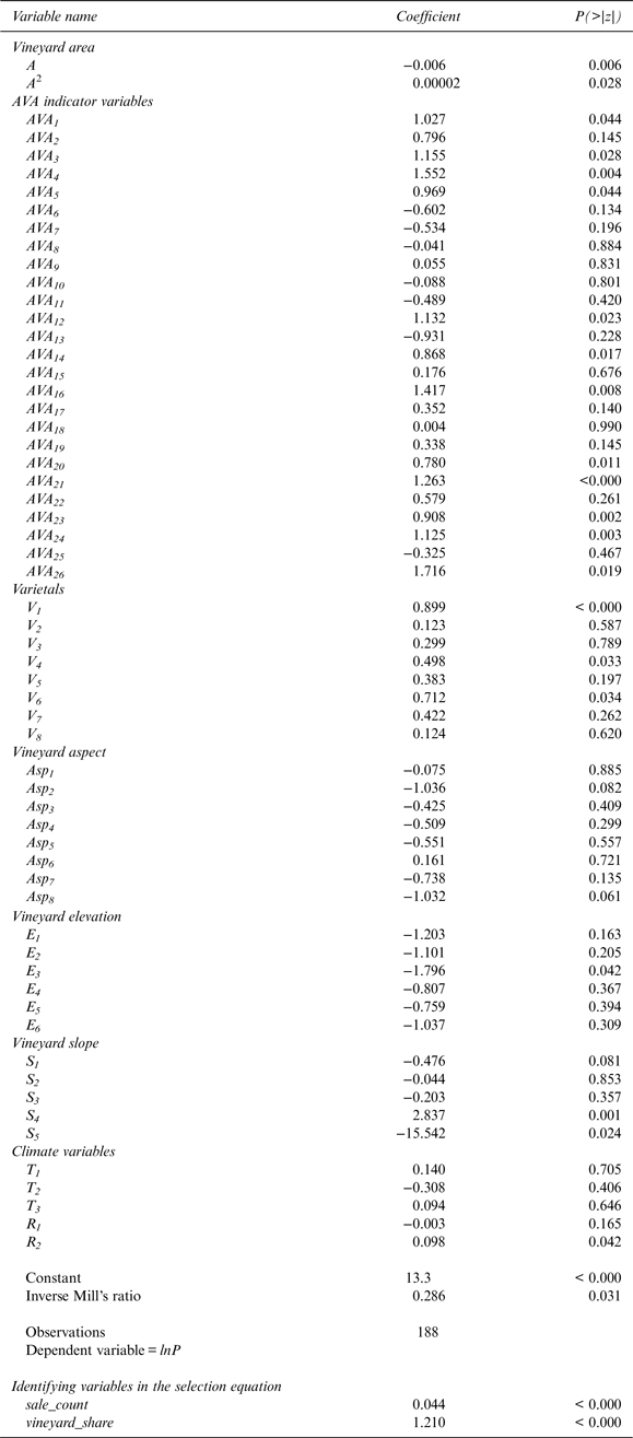
From the first stage, we construct the inverse Mill's ratio and include it as a variable in the hedonic price equation. As evidence of sample selection, note the significance of the coefficient on the inverse Mill's ratio (Melino, Reference Melino1982) in the second-stage hedonic regression—the z-value is 0.031 (Table 2). When the inverse Mill's ratio is omitted from the second-stage model, many of the coefficient estimates are smaller in absolute value and less precisely estimated. The key estimation results of both stages are reproduced in Table 2.
Table 2 Two-Stage Heckman Estimation Results
B. Results from the Hedonic Price Equation
Beginning with the site characteristics, the results indicate that some factors that would be assumed to contribute to terroir are significant, while others are not. In terms of effect of slope, there is a positive price premium for vineyards with a 20 to 30 degree slope (relative to flat ground), but a large negative effect for anything steeper. Although none of the aspect variables is significant, all the elevation variables are negative, with one category (200 to 300 feet) significant at the 5-percent level. Summer average precipitation has a positive and significant effect on vineyard prices, while none of the other climate variables is significant.Footnote 12
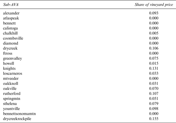
Turning to the viticultural area designations, most of the coefficients on the Sub-AVA indicator variables are positive, and nine are significantly different from zero (at the 5-percent confidence level), indicating price premiums for being inside many designated appellations. In seven cases, the estimated coefficients are negative, but none is significantly different from zero. The largest premiums are for the Knights Valley, Rutherford, and Dry Creek Sub-AVAs. Using the estimated parameters from the hedonic price model, calculated fitted values of the dependent variable provide estimates of the contribution that each Sub-AVA makes to vineyard sales prices (Table 3). These contributions to vineyard prices range from about 0 percent to nearly 16 percent.Footnote 13
Table 3 Estimated Contribution of Sub-AVAs to Vineyard Prices
C. Implications of the Results
In trying to sort out the meaning of terroir in the New-World context, the question we pose is essentially whether site attributes, AVA designations, or both influence vineyard prices. If site attributes affect wine quality (and if consumers are able to discriminate such quality), then vineyard prices depend on site attributes alone, because AVA designations are redundant. At the other extreme, if site attributes are irrelevant, with vineyard prices being fully explained by AVA designations, then terroir matters economically as a concept but not as a fundamental biophysical reality.
Our results support the intermediate case in which geographically based designations and some location-specific biophysical attributes are associated with the sales prices of vineyards. That said, the balance of the evidence supports the key role played by Sub-AVA designations, thereby supporting the notion that in Napa and Sonoma Counties, terroir matters economically as a concept but less so as a fundamental biophysical reality.
V. Conclusion
We have estimated a hedonic model of vineyard prices in one of the premier wine production areas of the New World—northern California's Napa and Sonoma Counties—to examine critically the notion of terroir, which plays such an important role in the production and appreciation of Old-World wines from the best locations in Europe. We examine whether Napa and Sonoma vineyard prices vary systematically with designated appellation, after controlling for site attributes.
Using precise measures of site attributes, we find mixed results—namely, that some site attributes have significant effects on vineyard sales prices, but others do not. The fact that some physical characteristics of vineyards are priced implicitly in the land market but others are not raises questions about whether Sub-AVA designations have a meaningful connection in reality with terroir. In our earlier study in Oregon, we reach a starker conclusion, finding that only AVA designations explain variation in vineyard prices.
We find more consistent results regarding designated appellations, with vineyard prices strongly affected by whether parcels are inside specific Sub-AVAs. This result indicates that terroir matters economically, with buyers and sellers of vineyard parcels in Napa and Sonoma Counties attaching significant premiums to specific designations. This is likely because consumers are willing to pay more for the experience of drinking wines from these areas. As studies using very different methodologies have found, although consumers may not discriminate much among wines in terms of their intrinsic qualities, they do respond to extrinsic attributes of wines, including prices and areas of origin.
In summary, site attributes and AVA designations influence vineyard prices, with estimated coefficients for site attributes measuring how producers value intra-AVA differences in vineyard characteristics. Producers attach premiums to site attributes that enhance wine quality if consumers can perceive and are willing to pay for such quality differences.
Data Appendix
Vineyard Sale Price
A detailed database of vineyard sales was obtained from an appraisal firm specializing in vineyards and wineries (Correia-Xavier, Inc., 2008). The database includes all vineyard sales in Napa and Sonoma Counties between 1991 and 2007. Appraised values are broken out for non-vineyard-related improvements, including residential and agricultural buildings, building site values, and winery permits. Vineyard sales values are obtained by removing any nonvineyard values from total sales prices and deflating to constant 2007 dollars using the Consumer Price Index.
Vineyard Boundaries
Improving on previous studies, we measure site attributes, such as climate, slope, aspect, and elevation, for the planted vineyards within each property instead of across the property as a whole. To obtain vineyard boundaries within sale parcels, we construct a digitized map of the sale parcel boundaries from historical Geographic Information System (GIS) records available at the Napa and Sonoma County Assessors’ Offices. Sales are matched to their digitized records using their Assessor Parcel Numbers (APNs) at the time of sale. The parcel map is then overlaid with digitized aerial photographs from county archives taken at or near the date of sale.Footnote 14 Vineyard boundaries are identified visually from the aerial images using GIS software (ArcGIS Version 10). Significant roads, driveways, trees, and outbuildings are excluded from vineyard areas.
We also generate a map of vineyard boundaries for all Napa and Sonoma Counties parcels, both sold and unsold. We obtain this census of vineyards by overlaying each county's APN layer with an aerial image, identifying vineyards visually, and delineating in ArcGIS. For this step, the aerial photo layers from 2000 and 2007 provide the best resolution for Sonoma and Napa Counties, respectively. For matching, APN boundary layers from 2000 and 2010 are used for Sonoma and Napa, respectively. A total of 10,323 vineyards is identified.Footnote 15
Vineyard Attributes
Another improvement over previous studies is the measurement of climatic variation across vineyards. Precipitation is measured for the effective growing season (February through September) as well as for the maturation and harvest period (July through September). Daily temperature fluctuation is measured for each month of the maturation and harvest period (July, August, and September). Daily climate observations are obtained from the PRISM Climate Group's 1980–present spatial climate database. Daily averages are calculated over the 10-year period of 1980 to 1989 to prevent overlap with the earliest vineyard sale database record.
Geographic attributes, including slope, aspect, and elevation, are obtained by dividing vineyards into 10-meter pixels and matching each pixel to its corresponding pixel in the National Elevation Dataset (U.S. Geological Survey, 2011). Each vineyard attribute, along with the two parcel-level sample-selection controls, including sales within a 2-kilometer buffer and the proportion of a parcel in vineyards, is calculated within the ArcGIS software environment.
The shares of vineyards located in specific AVAs and Sub-AVAs are determined by overlaying the vineyard boundary maps with digitized Sub-AVA maps for Napa and Sonoma Counties in ArcGIS. Public copies of the digitized AVA maps are made available by the two counties.


