II. California

In this section, we describe the regulatory environment for the beer market in California as well as illustrate the heterogeneity in consumer demographics across counties throughout California to motivate why this is a rich environment for study.

III. Demographics

With a population of over 39 million people, California would rank 34 in population and 5 in GDP for the world if viewed as an independent country. Furthermore, California has numerous counties that would rank in the top 100 countries in terms of GDP: Los Angeles (21), Santa Clara (37), Orange (49), San Diego (50), San Francisco (53), San Mateo (59), Alameda (59), San Bernardino (67), Sacramento (67), Riverside (70), and Contra Cosa (71). Indeed, California is a very diverse state with a lot of demographic and economic variation across counties. For a brief description of demographic summary statistics, see Table 1. It is also helpful to visualize spatially the variation in demographics across counties. Figure 1(a) shows how income per capita varies, while Figures 1(b)–(d) illustrate the variation among race/ethnicity.Footnote ¹

Figure 1. 2020 California county demographics. (a) Per Capita Income, (b) % White, (c) % Hispanic, (d) % Asian.

Table 1. 2020 County demographic summary statistics

Note: Population and personal income are in thousands.

IV. Data

California Business and Professions Code Section 25000 requires breweries, wholesalers, and importers to file beer price schedules with the California Department of Alcoholic Beverage Control (ABC). Until 2020, these price postings were all compiled in paper format, making them largely inaccessible to the general public. As the new system was launched, licensees were given the option to gradually phase into the online system, and as of October 15, 2023, they are now required to post all prices online. Starting on February 16, 2021, price postings were available online through ABC. This paper explores the first year of online observations, from February 2021 to June 2022. Prices are posted:

While the price posting data is transactional and displays package configuration and unit size, it does not include quantity sold, nor does it require an amendment every month that a malt beverage is sold if no attributes (including price) of the product change. In addition, transactions at multiple nodes in the beer supply chain may be recorded in the same period. For instance, a 12-pack of 12-oz aluminum cans of Sierra Nevada Pale Ale may be sold by the brewery to a wholesaler and then sold by the wholesaler to a retailer in the same county and month, such that both initial transactions will be recorded in the price posting data set. This particular aspect of the system allows for a glimpse into regional markups along the beer supply chain and potential differences between direct-to-consumer and conventional three-tier distribution. The price posting dataset contains multiple attributes of a particular malt beverage sold in California, including trade and product name, package configuration, product size, container type, destination county, buyer, price, and date.Footnote ²

To efficiently analyze the large dataset, extensive cleaning is conducted. All “non-beer” malt beverages such as seltzers, kombucha, and malt liquor are removed, as well as obvious entry errors such as incomplete filings. Package configuration is converted to one of three types: keg, loose, or pack. Total product size in ounces is calculated from Product Size and Package Configuration. Price per ounce is then calculated based on Price and total product size. Finally, we classify each beer’s ownership structure as Macro, defined as a brewery (or brewery conglomerate) with greater than 6 million barrels of annual production; Craft, as defined by the Brewers Association (2022); Crafty, as being a manufacturer with greater than 25% ownership by a non-alcohol manufacturing company or an alcohol manufacturing company that is not itself a craft brewery; and finally Import. With the price posting data cleaned, additional brewery and county descriptors are added.

The home county for California breweries is appended, as is the production size in 31-gallon barrels (bbls). This information comes from the California State Board of Equalization’s (CBOE) annual postings. County-level demographic data are merged as well. This information comes from the U.S. Bureau of Economic Analysis and provides county-level GDP, population, personal income, and race and age distributions.Footnote ³

Though the data is rich, there are some limitations. Essentially, the posting of a transaction is a registration to sell a particular package configuration in a county at a given price; quantities are not included. A brewery or distributer could post a price without actually selling in a county, such that we may observe a transaction in which 6x4 packs are sold and the price of that configuration, but we do not know how many 6x4 packs are sold in that transaction. Furthermore, we do not have the total universe of transactions. For example, there were 931 craft breweries in California in 2021, but we only have observations for 425 total breweries in California. This likely may be due to most breweries selling solely on their own premises. In addition, Bud Light (a truly ubiquitous beer) had price postings in only 25 counties during our observation timeline. This is likely because breweries are only required to file a transaction if something changes in that county, for example, price or package configuration. Thus, if neither of those things changes in the observation window, there will be missing observations.Footnote ⁴ Finally, though we observe when a new variety enters a market, we do not know when or if that variety leaves the market. This would be particularly useful information if one were to study the extensive margin of a brewery’s distribution.

V. Supply chain

Figure 2 illustrates the supply chain from Brewery to final destination. The way in which beer ends up at its final destination varies across types of breweries: macro, crafty, craft, and import. Table 2 breaks down the observations in the supply chain by type of beer. With self-distribution rights in California, a brewery can sell directly to consumers at their production facility or tap room, directly to retailers, either for on-premise consumption at pubs or restaurants, or for off-premise consumption at grocery or liquor stores, to wholesale distributers that will then sell to retailers, or to federal enclaves that operate their own retail establishments. The California price posting data allows us to observe transactions at every point on this supply chain except for brewery sales direct to consumers.Footnote ⁵ In addition, lateral flows of goods are recorded. Transactions such as a brewery selling to another brewery, as is the case when one brewery may feature another in their tap room, or an importer selling to a distributer are illustrated in Table 2.

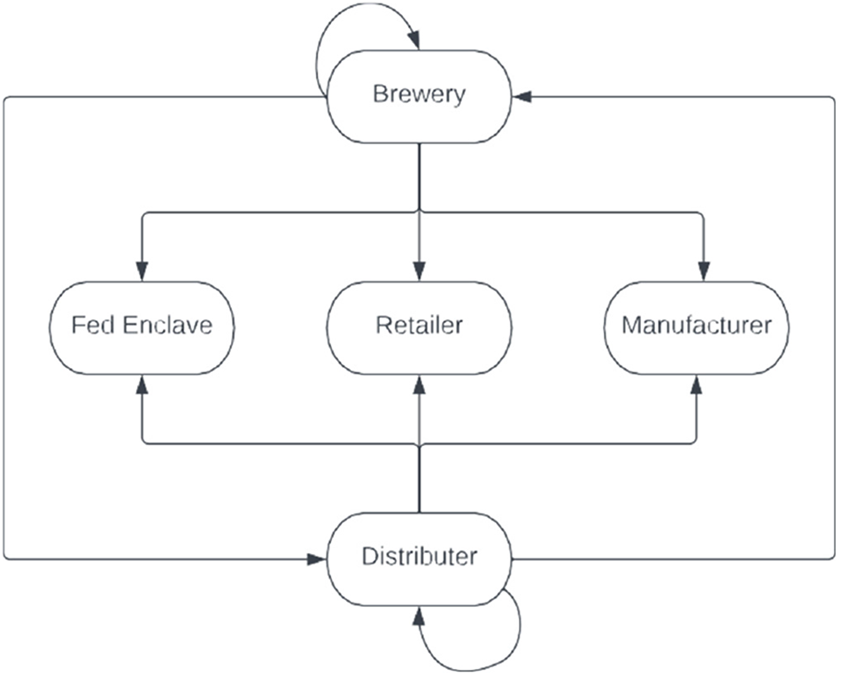
Figure 2. Supply chain flow.

Table 2. Transactions in supply chain by type

Note: See the text for the definition of “Crafty.”

Craft beer has by far the largest volume of observations in the price posting data. While they make up the largest sector of breweries in terms of establishments and beers made, they currently only hold slightly over 13% of the national market in terms of volume (BA 2022). In addition, craft breweries tend to continuously change product lines and recorded an average of 81.74 varieties with price postings over the sample period. Crafty breweries registered 74.74 on average per brewery, while macro and import only registered 11.25 and 9.71, respectively.

We also illustrate the variation in package type across the supply chain in Table 3. Note that a large percentage of observations of keg and pack go from either a brewery straight to retail or a distributer. Moreover, bottles are nearly entirely sold directly from a brewery to a retailer, as well as zero observations of loose packaging sold either from a distributer to a brewery or a federal enclave, or from a brewery directly to a federal enclave. This nuance will be important in order to properly isolate the effect of where in the supply chain the transaction occurs on the price per ounce.

Table 3. Supply chain by package type

VI. California breweries

In this section, we provide some descriptive statistics regarding California breweries. Of the nearly 900 breweries that currently operate in California, only 425 California breweries have listed transactions in our sample. This fraction of breweries in the posting data is likely due to two reasons. First, there are over 600 breweries operating that sell more than 25% of their production onsite, which does not require transaction reports. Second, the breweries might not have new accounts and/or price adjustments during the collection period.

Of the total varieties sold by the 425 CA breweries, 0.3% went to federal enclaves, 0.6% went to manufacturers, 69% went to retailers, and 30% went to wholesalers. The breakdown of supply chain distribution is quite similar to the average across breweries (Table 4). The two largest arms again are brewery direct to retail at 56% and brewery to wholesale at 30%. Interestingly, brewery-to-brewery sales average 0.5% across CA breweries, with a maximum of 1, indicating that there was at least one California brewery that sold all its beers to another brewery.

Table 4. California brewery summary statistics

For California-produced beers, the average price per ounce across all transactions was approximately $0.14, or $2.24 per pint. We further discuss price differentials in the next section. In terms of packaging, the majority of price posting transactions were in the form of kegs at 66.7%. This is not surprising, as this is the common form of packaging used in on-premise consumption at pubs and restaurants. Packs in various forms follow at 30.2%, in most cases intended for off-premise consumption. Individual bottle sales and loose cans make up the remainder at 1.8% and 1.3%, respectively. Finally, on average, a California brewery has beer registered to be served in just over half, 30.66 of 58, of all California counties during our sample period.

Examining individual California breweries provides some valuable insight into the relationship between small, micro, and regional craft breweries’ decisions to distribute beer. Figure 3 provides the percentage of product line price postings for four California breweries of varying size and location: Central Coast Brewing, Firestone Walker Brewing, Modern Times, and Russian River Brewing Company. Modern Times distribution, headquartered in San Diego, is the bottom left figure. In 2021, their total production was about 53,000 bbls and they distributed 135 varieties from February 2021 to June 2022. In addition to distribution, Modern Times ran six brewpub/taprooms in Southern California and one in Oregon State. Post-pandemic shutdowns and the company selling to another craft brewery have forced them to close three of their locations and rethink their business model. Note that for the 135 beer varieties they distributed in 2021/22, most counties that had registered beer obtained a large proportion of their varieties.

Figure 3. Percent of product line sold. (a) Central Coast Brewing, (b) Firestone Walker, (c) Modern Times, (d) Russian River.

Russian River Brewing, most famous for their Pliny the Elder and Pliny the Younger beers, produced about 70% as much as Modern Times and distributed 81 varieties (60%) in the same time frame. In addition, their distribution scheme appears much more targeted, concentrating mainly in surrounding Bay Area counties and then up and down the coast. Next, Central Coast Brewing, while only producing 2,727 bbls, registered 64 varieties. Note that their distribution is very localized, with surrounding counties receiving 65–100% of varieties and the rest of the state receiving less than 20%. Finally, contrast the three relatively small craft breweries to one of the largest breweries in California, Firestone Walker, owned by Belgian brewers Duvel Moortgat. Their 2021 production was 528,188 barrels with 135 varieties. The concentration of beers sold in the counties where they are sold is quite dichotomous. It appears they either registered nearly all varieties in a county or hardly any. Again, this may be due to data limitations where transactions could have occurred in the time frame but were not recorded because price or packaging did not change. Regardless, as more data becomes available, this avenue of examining the price posting data will afford a better understanding of brewers’ distribution decision-making.

In Table 5, we run a simple regression on the percent of a brewery’s product line sent to each county to highlight the heterogeneity in supply decisions.Footnote ⁶ As expected, we find that this percent decreases in the bilateral distance from the home county. However, the more counties a brewery has a presence in, the greater the percent of the product line that is supplied. There is a negative effect on production size, perhaps indicating that larger craft breweries tend to be more targeted in their distribution.Footnote ⁷

Table 5. Percent of product line sent to each county

Notes: Robust standard errors in parentheses:

*** p < 0.01, **p < 0.05, *p < 0.1. Source and destination county FE are included.

VII. Pricing

This section investigates the pricing strategy of a brewery. PricePerOunce_ijvghdt is a unit of observation, where i is the source county (missing if outside of California), j is the destination county, v is the variety (name) of beer, g is the “Product” (which represents product configuration, unit size, and container type), h is where it is in the supply chain, d is whether it’s delivered or FOB, and t is time (calendar date). Before exploring all the determinants of pricing, we first explore possible “pricing to market.” The descriptive analysis of variation across counties within California helps motivate potential variation in demand by location. However, recall that our data does not include the total quantity sold to each county, so while it is likely there are differences in quantity sold, it is not entirely clear that prices will also vary across counties. The next subsection explores this possibility and helps motivate the use of county fixed effects in our pricing model.

a. Pricing to market

Even within a single year of observations, the new price posting dataset allows for a geographic exploration of brewers’ and wholesalers’ pricing strategies and how they may differ across brewery sizes.Footnote ⁸ Take as a unit of observation the price per ounce for a variety to a buyer in the supply chain in a particular county in a particular month for a particular package configuration/size/container type. Define CV Price as the coefficient of variation of prices/oz for a variety to a buyer in the supply chain for a particular month, product (grouping of package configuration, unit size, and container type). Thus, for a given variety/product/supply chain/month/delivery, this will give us the standard deviation in prices relative to the mean. In other words, if CV_Price = 0, then the variety is the same price per oz across counties; if CV_Price > 0, then there is “pricing-to-market.” Table 6 gives summary statistics of this variation in price per ounce across counties. Without any additional controls, macro beer has the highest average variation in prices relative to the mean across counties, followed by crafty beer and then imported beer. Craft beer has the lowest average coefficient of variation, which suggests craft beer participates in less “pricing-to-market” as is to be expected since they typically have had less access to information on competitive prices in a market, a point that is no longer the case with the publishing of this dataset.

Table 6. Coefficient of variation in price by type

Though Table 6 provides some evidence of variation in pricing to market strategies by type, it is important to control for other aspects, like the supply chain. Table 7 provides such an analysis. We regress the coefficient of variation of price per ounce across counties controlling for terms of sale: delivery/FOB; location in the supply chain; and the type of beer (macro, crafty, craft, or import) with product and month fixed effects and clustered standard errors at the product level (recall “product” is the grouping of package configuration, unit size, and container type). Our first specification includes the full sample, while the next four specifications break up the sample by brewery type. Relative to macro beer, craft beer has a negative and statistically significant coefficient. We interpret this as craft beer engaging in less pricing to market relative to macro, crafty, and imported beer. Again, one possible explanation is that craft breweries are predominantly much smaller operations and do not have the resources to determine optimal prices for each market. We also break up the data across brewery types and can see that, relative to sales to a distributer/wholesaler, craft beer has less price variation across counties throughout the supply chain.

Table 7. Coefficient of variation in price per ounce across counties

Notes: Robust standard errors in parentheses:

*** p < 0.01, **p < 0.05, *p < 0.1. Product and month FE are included. Standard errors are clustered at the tradename level.

b. Price determinants

When thinking about the determinants of prices, we are primarily interested in how the location in the supply chain affects the pricing decision as well as the packaging (keg versus bottle, can, and pack) and the type of beer (macro versus crafty, craft, and imported). We have been motivated in our description of the California market in Section 2 as well as the previous subsection, Section 7a, that one would expect variation across counties, and thus it would be appropriate to include county fixed effects. We further illustrate in Figure 4 that there is variation across months and that “seasonal” effects are present. Though keg prices seem fairly stable, there is more variation with bottle and can prices. At first glance, one might infer that on average, keg prices are lower than bottles and cans. However, we will address this more formally with robust empirical analysis. In the remaining analysis, we omit observations with a price per oz above $0.28879—that is, the top 5% outliers. This is an attempt to eliminate special release/anniversary beers from our analysis.Footnote ⁹

Figure 4. Prices by month. (a) Bottle Price, (b) Keg Price, (c) Can Price.

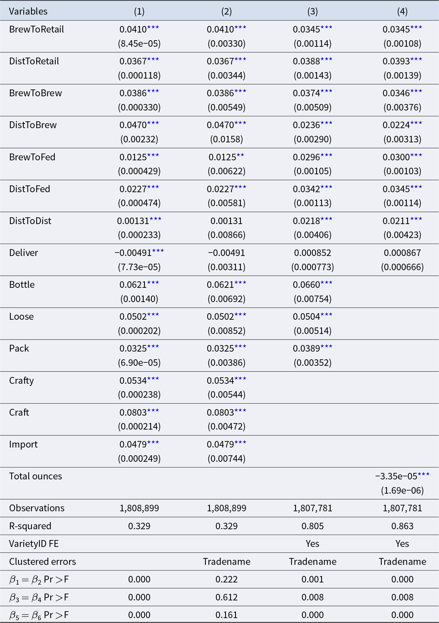
We present four different specifications in Table 8. The first includes county and month fixed effects but does not cluster standard errors. Finding the appropriate level to cluster errors can be debatable (see Abadie et al., Reference Abadie, Athey, Imbens and Wooldridge2023). We have chosen to cluster standard errors at the tradename level, as it seems reasonable that there may be some correlation at this level in pricing strategies across the firm’s product line. Another possibility would be at the manufacturer level, as some manufacturers have multiple trade names, for example, Anheuser-Busch. However, we postulate that any pricing strategies will more likely be at the tradename level; further exploration into pricing strategy differentials between trade name and manufacturer may be a worthwhile endeavor now possible with this dataset.Footnote ¹⁰ Specification (2) clusters standard errors, and all coefficients maintain significance with the exception of DistToDist and Deliver. Specifications (3) and (4) add in product name (VarietyID) fixed effects, and Specification (4) includes the variable Total Ounces instead of the package-type binary variables.Footnote ¹¹ We also omit the binary variable CA that indicates whether the brewery is home to California since there would likely be too much multicollinearity between this and Craft breweries, as the predominant type of brewery in California is Craft.Footnote ¹²

Table 8. Price per ounce

Notes: Robust standard errors in parentheses:

*** p < 0.01, **p < 0.05, *p < 0.1. County and month FE are included.

Unsurprisingly, relative to kegs, all other packaging types (bottle, loose, and pack) are more expensive per ounce, with single bottles being the most expensive. It is also expected that macro is the cheapest per ounce while craft and crafty are about the same, which is confirmed by our analysis. The results become more interesting when looking at the different markups relative to wholesale prices.Footnote ¹³ At the aggregate level, when controlling for variety fixed effects, there is about a half-penny discount per oz (or $0.06 per 12-oz beer) when going straight to a retailer or federal enclave from the brewery. When supplying to a brewery, the markup seems to be higher when coming straight from another brewery. However, this could be a selection issue that is not being accounted for, as these might be more collaborations on special releases.

Given the variation across package and brewery types and the fact that our observations overwhelmingly come from craft breweries, it would be prudent to analyze the data accounting for brewery type.Footnote ¹⁴ Instead of including many interaction terms, we run our specification for each subgroup separately. We report this analysis in Table 9 with variety-fixed effects.Footnote ¹⁵ Here we begin to see the heterogeneity between beer types. Of particular interest is the effect of “cutting out the middleman” when supplying to retailers. Though the markups over wholesale prices are smaller for macro beers, the “discount” is about the same in levels. This half-penny discount is maintained for craft and import beers, while crafty beers are essentially the same. It can also be seen that the difference in markups to federal enclaves is really being driven by craft beer sales, as is the difference in markups to breweries.

Table 9. Price per ounce by type with variety fixed effects

Notes: Robust standard errors in parentheses:

*** p < 0.01, **p < 0.05, *p < 0.1. County, month, and variety FE are included. Standard errors clustered at the tradename level.

Table 10. Observations by packaging/brewery type

We have highlighted the degree of heterogeneity across brewery types, but it is also important to note the heterogeneity across packaging types as well. In the Appendix, we illustrate such heterogeneity with regard to the pricing structure. In Tables 11 and 12, we break the pricing strategy down further by packaging type; specifically, we focus on kegs and packs. Though qualitative results are similar, this highlights that the entire pricing strategy depends on both brewery and packaging types.

Table 11. Price per ounce for kegs by type

Notes: Robust standard errors in parentheses:

*** p < 0.01, **p < 0.05, *p < 0.1. County and month FE are included. Standard errors clustered at the tradename level.

Table 12. Price per ounce for packs by type

Notes: Robust standard errors in parentheses:

*** p < 0.01, **p < 0.05, *p < 0.1. County and month FE are included. Standard errors clustered at the tradename level.