1 Introduction
High-energy emission in pulsars comes from high altitudes. Recent work shows that most optical, X-ray and
 ${\it\gamma}$
-ray emission comes from caustic zones at mid-to-high altitudes in the star’s magnetosphere or wind. The details, however, remain unclear. The high-energyFootnote
1
emission zones can lie anywhere along or within the open field line zones which exist over the star’s magnetic poles. They may also coincide with current sheets either within or outside of the light cylinder. The highly nonlinear behaviour of relativistic photon caustics, combined with uncertainties in the magnetic field structure close to the light cylinder, means that any of these possible emission zones can reproduce observed high-energy light curves. Because we do not know whether pulsed high-energy emission is due to synchrotron radiation, curvature radiation or inverse Compton scattering, we have few constraints on physical conditions within the high-energy emission zones. We need more information, and believe radio observations can help.
${\it\gamma}$
-ray emission comes from caustic zones at mid-to-high altitudes in the star’s magnetosphere or wind. The details, however, remain unclear. The high-energyFootnote
1
emission zones can lie anywhere along or within the open field line zones which exist over the star’s magnetic poles. They may also coincide with current sheets either within or outside of the light cylinder. The highly nonlinear behaviour of relativistic photon caustics, combined with uncertainties in the magnetic field structure close to the light cylinder, means that any of these possible emission zones can reproduce observed high-energy light curves. Because we do not know whether pulsed high-energy emission is due to synchrotron radiation, curvature radiation or inverse Compton scattering, we have few constraints on physical conditions within the high-energy emission zones. We need more information, and believe radio observations can help.
Radio emission in a large number of pulsars comes from lower altitudes, close to the magnetic axis. This geometry works for many pulsars, but fails for an interesting minority. For those stars – including the pulsar in the Crab Nebula, the subject of this paper – the similarity of the radio and high-energy light curves strongly suggests the radio emission comes from the same high-altitude regions that create the high-energy emission. However, the geometrical models do not address the physical mechanisms by which the magnetospheric plasma produces the intense radio emission we observe. Many different emission mechanisms have been proposed, but none has been proven to be operating in the general pulsar population.
Our group has approached the question of pulsar radio emission mechanisms by carrying out detailed studies of one object, the Crab pulsar. This pulsar shines in radio at many phases throughout its rotation period, with seven components detectable in its mean profileFootnote 2 . At least three, and probably five, of these come from high-altitude emission zones, spatially coincident with the high-energy emission zones in this star’s magnetosphere. The high time resolution and broad spectral bandwidth of our observations show that different components have different temporal and spectral characteristics. We infer that more than one type of radio emission mechanism is taking place within the star’s magnetosphere.
In this paper we collect and review our observational results, compare them to competing radio emission models and from this comparison discuss what physical conditions exist in the high-altitude zones that emit both radio and high-energy pulsed emission. We begin in § 2 by reviewing the basic picture of the rotating pulsar magnetosphere and its modern extension to the high-altitude transition to the wind zone. We focus on where in the extended magnetosphere the radio and high-energy emission originate. In § 3 we lay out physical conditions that must exist (the ‘emission physics’) if the magnetosphere is to produce intense radio emission. In § 4 we set the stage for our discussion of the radio properties of the Crab. We present the different components of the mean radio profile and review our observations of the pulsar. In § 5 we focus on the Main Pulse and the Low Frequency Interpulse, which we believe involve similar emission physics. Both of these components show bursting behaviour on sub-microsecond time scales; we argue this reflects variability of the driving mechanism, which is probably due to unshielded electric fields local to the region. We also introduce nanoshots – flares of emission on nanosecond time scales – which we believe reveal the fundamental emission process in these components. In § 6 we compare observed nanoshot properties to predictions of three plausible radio emission models. Although none of the models can fully explain the data, we suggest they can be used to constrain physical conditions in the radio emission zones. We then switch to the High requency Interpulse, a separate component with different radio characteristics that very likely involves different emission physics. In § 7 we discuss its radio properties, including the unexpected spectral emission bands, and consider what emission physics might be responsible for the bands. In § 8 we present two additional clues to its local environment: signal dispersion and polarization angle. Finally, in § 9, after congratulating the steadfast reader who has made it to the end, we end by summarizing the lessons we have learned to help us going forward.
We relegate to the Appendices necessary details on a variety of possible radio emission mechanisms. In appendix A we briefly review specific models of coherent radio emission that have been proposed for the general pulsar population, and in appendix B we review one additional model specifically proposed for the High Frequency Interpulse of the Crab pulsar.
2 Emission zones in the pulsar magnetosphere
Consider a rapidly rotating neutron star which supports a strong magnetic fieldFootnote
3
above the star’s surface. Within the so-called ‘light cylinder’ – the radius at which the corotation speed becomes the speed of light – the magnetic field geometry is thought to be nearly that of a vacuum dipole, rotating with the star and having its magnetic moment oriented at some oblique angle to the star’s rotation axis. Approaching the light cylinder, relativistic effects ‘sweep back’ the dipolar field lines, generating a toroidal component which becomes an outward propagating EM wave past the light cylinder (Deutsch Reference Deutsch1955). Most poloidal field lines which leave the star’s surface return to the pulsar well within the light cylinder, creating the ‘closed field zone’. It is generally thought that plasma in this region, pulled from the star’s surface by rotation-induced electric fields, becomes charge separated in just the amount needed to short out any parallel electric field. This necessary charge density is known as the ‘Goldreich–Julian charge density’,
 $n_{GJ}={\it\Omega}_{\ast }\boldsymbol{\cdot }\boldsymbol{B}/2{\rm\pi}ec$
, from a seminal ansatz by Goldreich & Julian (Reference Goldreich and Julian1969, ‘GJ’). If this density is attained, it supports corotation of a force-free plasma magnetosphere in the closed field line region. It is also generally agreed that magnetic field lines or flux ropes which originate near the star’s magnetic poles cross the light cylinder before they return to the star, creating an ‘open field line’ region. The area on the star’s surface traced by the outermost open field lines is called the ‘polar cap’.
$n_{GJ}={\it\Omega}_{\ast }\boldsymbol{\cdot }\boldsymbol{B}/2{\rm\pi}ec$
, from a seminal ansatz by Goldreich & Julian (Reference Goldreich and Julian1969, ‘GJ’). If this density is attained, it supports corotation of a force-free plasma magnetosphere in the closed field line region. It is also generally agreed that magnetic field lines or flux ropes which originate near the star’s magnetic poles cross the light cylinder before they return to the star, creating an ‘open field line’ region. The area on the star’s surface traced by the outermost open field lines is called the ‘polar cap’.
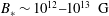
Table 1. Scaling numbers for the Crab pulsar, assuming the Goldreich–Julian (‘GJ’, § 2) model holds.
 ${\it\nu}_{B}$
is the lepton Larmor frequency;
${\it\nu}_{B}$
is the lepton Larmor frequency;
 ${\it\nu}_{p}$
is the lepton plasma frequency. Values are given at the star’s surface and at two higher altitudes more relevant to the radio and high-energy emission.
${\it\nu}_{p}$
is the lepton plasma frequency. Values are given at the star’s surface and at two higher altitudes more relevant to the radio and high-energy emission.
 $R_{\ast }\simeq 10$
km is the radius of the neutron star, which rotates at
$R_{\ast }\simeq 10$
km is the radius of the neutron star, which rotates at
 ${\it\Omega}_{\ast }\simeq 190~\text{rad}~\text{s}^{-1}$
(rotation period 33 ms). The distance
${\it\Omega}_{\ast }\simeq 190~\text{rad}~\text{s}^{-1}$
(rotation period 33 ms). The distance
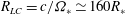 $R_{LC}=c/{\it\Omega}_{\ast }\simeq 160R_{\ast }$
is the light cylinder radius. The magnetic field is assumed to be dipolar. The number density of charge required to maintain corotation is
$R_{LC}=c/{\it\Omega}_{\ast }\simeq 160R_{\ast }$
is the light cylinder radius. The magnetic field is assumed to be dipolar. The number density of charge required to maintain corotation is
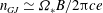 $n_{GJ}\simeq {\it\Omega}_{\ast }B/2{\rm\pi}ce$
. In many applications the number density of the plasma is thought to be enhanced relative to the GJ value, by a factor
$n_{GJ}\simeq {\it\Omega}_{\ast }B/2{\rm\pi}ce$
. In many applications the number density of the plasma is thought to be enhanced relative to the GJ value, by a factor
 ${\it\lambda}=n/n_{GJ}$
.
${\it\lambda}=n/n_{GJ}$
.

This model is hardly the final word on the subject. The structure of the magnetosphere is complex, dynamic and nonlinear. It is far from clear that it will ever attain the steady-state situation envisaged by Goldreich & Julian, because magnetic fields, currents and charges feed back on each other, creating a very dynamic system. Observations reveal that the radio emission is variable on both short and long time scales; this also suggests that the emission regions are unsteady and dynamic. Nonetheless, the model provides valuable insights, and it has become part of the ‘standard pulsar picture’ over the years. To illustrate the model, and for later reference for the Crab pulsar, we list important scaling numbers in table 1.
2.1 The traditional radio geometry: lighthouse beams
The picture just described has been particularly successful in providing a context for understanding the pulsed radio emission by which most pulsars have been discovered. Plasma/current flow out along the open field lines enables the build up of charge-starved regions (so-called ‘gaps’). Such gaps may fill the open field line region close to the star’s surface (polar gap; e.g. Ruderman & Sutherland Reference Ruderman and Sutherland1975), or may sit along the edge of the open field line region (slot gap; Arons & Scharlemann Reference Arons and Scharlemann1979). Parallel electric fields (
 $E_{\Vert }$
; component along
$E_{\Vert }$
; component along
 $\boldsymbol{B}$
) in these gaps accelerate outflowing charges to very high Lorentz factors (typically
$\boldsymbol{B}$
) in these gaps accelerate outflowing charges to very high Lorentz factors (typically
 ${\it\gamma}\sim 10^{6}{-}10^{7}$
). Curvature radiation from these fast charges supports magnetic pair creationFootnote
4
in the strong magnetic field close to the polar cap. The pair cascade enhances the plasma density, relative to
${\it\gamma}\sim 10^{6}{-}10^{7}$
). Curvature radiation from these fast charges supports magnetic pair creationFootnote
4
in the strong magnetic field close to the polar cap. The pair cascade enhances the plasma density, relative to
 $n_{GJ}$
, by a factor
$n_{GJ}$
, by a factor
 ${\it\lambda}=n/n_{GJ}$
. Models suggest
${\it\lambda}=n/n_{GJ}$
. Models suggest
 ${\it\lambda}\sim 10^{2}{-}10^{4}$
, and a final pair streaming speed
${\it\lambda}\sim 10^{2}{-}10^{4}$
, and a final pair streaming speed
 ${\it\gamma}_{s}\sim 10^{2}{-}10^{3}$
(Hibschman & Arons Reference Hibschman and Arons2001; Arendt Jr & Eilek Reference Arendt and Eilek2002). Thus, result of the pair cascade is a fast particle beam moving through a slower moving pair plasma, both still moving out along the open field lines.
${\it\gamma}_{s}\sim 10^{2}{-}10^{3}$
(Hibschman & Arons Reference Hibschman and Arons2001; Arendt Jr & Eilek Reference Arendt and Eilek2002). Thus, result of the pair cascade is a fast particle beam moving through a slower moving pair plasma, both still moving out along the open field lines.
If some part of the energy in the fast outflow through the open field line region is converted to radio emission – which will be strongly forward beamed, approximately along the star’s magnetic axis – an observer will see a radio pulse every time the star’s rotation sweeps this ‘lighthouse beam’ past his or her sightline. In this simple picture, most pulsars should show only one pulse per rotation period, which is indeed the case. We would need a special geometry to see more: either the magnetic moment and the viewing angle are both at
 $90^{\circ }$
to the rotation axis (giving two pulses
$90^{\circ }$
to the rotation axis (giving two pulses
 $180^{\circ }$
apart) or both are very close to the rotation axis (giving a complex pulse distribution if the emitting region is inhomogeneous). This model also predicts the position angle of linear polarization should rotate as the radio beam crosses the observer’s sightline (Radhakrishnan & Cooke Reference Radhakrishnan and Cooke1969; assuming the polarization direction is rigidly tied to magnetic field geometry in the emission zone). Because both predictions hold true for the majority of well-studied pulsars, this geometry has become part of the standard pulsar picture for the past several decades.
$180^{\circ }$
apart) or both are very close to the rotation axis (giving a complex pulse distribution if the emitting region is inhomogeneous). This model also predicts the position angle of linear polarization should rotate as the radio beam crosses the observer’s sightline (Radhakrishnan & Cooke Reference Radhakrishnan and Cooke1969; assuming the polarization direction is rigidly tied to magnetic field geometry in the emission zone). Because both predictions hold true for the majority of well-studied pulsars, this geometry has become part of the standard pulsar picture for the past several decades.
2.2 Expand this picture: the extended magnetosphere
We’ve learned much more in recent years. The happy conjunction of abundant high-energy pulsar observations with significant advances in numerical simulations (both MHD and PIC methods) have greatly broadened our understanding of the high-altitude magnetosphere and its transition to the pulsar wind (known as the ‘extended’ magnetosphere; e.g. Kalapotharakos, Contopoulos & Kazanas Reference Kalapotharakos, Contopoulos and Kazanas2012a
). Various analytic attempts to understand the region around the light cylinder have generally proved less than successful over the years, but several groups have now modelled this region numerically. Initial numerical work assumed pair creation was sufficiently abundant that the force-free condition (
 $\boldsymbol{E}\boldsymbol{\cdot }\boldsymbol{B}=0$
) holds everywhere (e.g. Bai & Spitkovsky Reference Bai and Spitkovsky2010; Contopoulos & Kalapotharakos Reference Contopoulos and Kalapotharakos2010). More recently, modelling has been extended to include phenomenological resistivity in regions where current sheets are expected (e.g. Kalapotharakos et al.
Reference Kalapotharakos, Kazanas, Harding and Contopoulos2012b
; Li, Spitkovsky & Tchekhovskoy Reference Li, Spitkovsky and Tchekhovskoy2012).
$\boldsymbol{E}\boldsymbol{\cdot }\boldsymbol{B}=0$
) holds everywhere (e.g. Bai & Spitkovsky Reference Bai and Spitkovsky2010; Contopoulos & Kalapotharakos Reference Contopoulos and Kalapotharakos2010). More recently, modelling has been extended to include phenomenological resistivity in regions where current sheets are expected (e.g. Kalapotharakos et al.
Reference Kalapotharakos, Kazanas, Harding and Contopoulos2012b
; Li, Spitkovsky & Tchekhovskoy Reference Li, Spitkovsky and Tchekhovskoy2012).
While details differ between authors, the basic properties of the extended magnetosphere seem to be agreed on, and are in good agreement with the analytic models of Bogovalov (Reference Bogovalov1999). Closed field lines and charge-separated regions exist within light cylinder, as predicted by the GJ model. Plasma flows out along open field lines, crosses the light cylinder and develops into an outflowing pulsar wind. Past the light cylinder, the plasma flow – which must remain below the speed of light – trails the star’s rotation and creates a spiral pattern for the toroidal magnetic field. The poloidal field becomes asymptotically radial and develops a ‘split monopole’ structure, changing sign across an undulating equatorial current sheet. This picture of the extended magnetosphere reveals more regions which may accelerate particles to relativistic energies and have the potential to be emission zones for high-energy emission, radio emission or both.
Gaps are regions where force-free MHD breaks down and unshielded
 $E_{\Vert }$
can exist; a variety of explanations have been suggested. In addition to the low-altitude polar gaps described above, some authors have suggested slot gaps, which extend the polar gap from the star’s surface out to the light cylinder along the edges of the open field line region (Arons & Scharlemann Reference Arons and Scharlemann1979; Muslimov & Harding Reference Muslimov and Harding2004; also called two-pole caustics, see next section). Other authors have suggested outer gaps and annular gaps: vacuum regions allowing
$E_{\Vert }$
can exist; a variety of explanations have been suggested. In addition to the low-altitude polar gaps described above, some authors have suggested slot gaps, which extend the polar gap from the star’s surface out to the light cylinder along the edges of the open field line region (Arons & Scharlemann Reference Arons and Scharlemann1979; Muslimov & Harding Reference Muslimov and Harding2004; also called two-pole caustics, see next section). Other authors have suggested outer gaps and annular gaps: vacuum regions allowing
 $E_{\Vert }\neq 0$
, originating close to the so-called neutral charge surface (part way out along the open field region, where the charge density needed for corotation changes sign) and extending by some distance both towards the light cylinder and into the polar flux tube (e.g. Cheng, Ho & Ruderman Reference Cheng, Ho and Ruderman1986; Romani & Yadigaroglu Reference Romani and Yadigaroglu1995; Qiao et al.
Reference Qiao, Lee, Wang, Xu and Han2004).
$E_{\Vert }\neq 0$
, originating close to the so-called neutral charge surface (part way out along the open field region, where the charge density needed for corotation changes sign) and extending by some distance both towards the light cylinder and into the polar flux tube (e.g. Cheng, Ho & Ruderman Reference Cheng, Ho and Ruderman1986; Romani & Yadigaroglu Reference Romani and Yadigaroglu1995; Qiao et al.
Reference Qiao, Lee, Wang, Xu and Han2004).
Current sheets have also been suggested as possible sites of particle energization and high-energy radiation. In models of the extended magnetosphere, current sheets exist both within the light cylinder – where currents flow along the separatrices between open and closed field lines – and external to the light cylinder – where an undulating current sheet, frozen into the wind, separates the two hemispheres of the split monopole wind. It is often argued that reconnection events across the current sheets energize the plasma, possibly to relativistic energies, making them additional sources of high-energy emission (e.g. Petri & Kirk Reference Pétri and Kirk2005; Bai & Spitkovsky Reference Bai and Spitkovsky2010; Cerutti et al. Reference Cerutti, Philippov, Parfrey and Spitkovsky2015). Although we have not seen much discussion of these current sheets as sites of radio emission, we think the topic warrants further study.
2.3 Caustics, sky maps and high-energy emission
Rapid recent advances in high-energy pulsar observations – particularly the many
 ${\it\gamma}$
-ray light curves obtained by Fermi (Abdo et al.
Reference Abdo, Ajello, Baldini, Ballet, Barbiellini, Baring, Bastieri, Belfiore and Bellazzzini2013) – reveal that double-peaked high-energy pulsar light curves are the rule rather than the exception. This shows that high-energy emission cannot come from low altitudes, because there are far too many double-peaked high-energy light curves to be consistent with the special geometry needed (both viewing and inclination angles close to
${\it\gamma}$
-ray light curves obtained by Fermi (Abdo et al.
Reference Abdo, Ajello, Baldini, Ballet, Barbiellini, Baring, Bastieri, Belfiore and Bellazzzini2013) – reveal that double-peaked high-energy pulsar light curves are the rule rather than the exception. This shows that high-energy emission cannot come from low altitudes, because there are far too many double-peaked high-energy light curves to be consistent with the special geometry needed (both viewing and inclination angles close to
 $90^{\circ }$
) if the emission were from low-altitude polar gaps. It is now generally accepted that the two bright peaks typical of high-energy light curves come from extended high-altitude regions – gaps or current sheets – associated with, but not local to, the star’s two magnetic poles.
$90^{\circ }$
) if the emission were from low-altitude polar gaps. It is now generally accepted that the two bright peaks typical of high-energy light curves come from extended high-altitude regions – gaps or current sheets – associated with, but not local to, the star’s two magnetic poles.
The detailed structure of these high-altitude emission regions is not understood and cannot easily be determined from observations. Finite photon light travel times, and the non-dipolar magnetic field geometry at high altitudes, cause outgoing photons emitted parallel to
 $\boldsymbol{B}$
to accumulate in a few preferred directions (‘caustics’). Simulations document a highly nonlinear mapping between the spatial structure of magnetospheric emission regions and the rotation phases and viewing angles at which emitted radiation is caught by the observer. In particular, double-peaked light curves do not require special geometry, but are seen from a wide range of viewing and orientation angles (e.g. Dyks, Harding & Rudak Reference Dyks, Harding and Rudak2004; Bai & Spitkovsky Reference Bai and Spitkovsky2010).
$\boldsymbol{B}$
to accumulate in a few preferred directions (‘caustics’). Simulations document a highly nonlinear mapping between the spatial structure of magnetospheric emission regions and the rotation phases and viewing angles at which emitted radiation is caught by the observer. In particular, double-peaked light curves do not require special geometry, but are seen from a wide range of viewing and orientation angles (e.g. Dyks, Harding & Rudak Reference Dyks, Harding and Rudak2004; Bai & Spitkovsky Reference Bai and Spitkovsky2010).
How does all this connect to radio emission? In many pulsars, the radio and high-energy light curves are out of phase with the main radio pulse, leading the brighter of the two high-energy pulses by 0.2–0.3 of a rotation period. This is generally ascribed to radio emission coming from low-altitude polar gaps, while high-energy emission comes from high altitudes. Because the emission mechanisms are also different, one might think the radio and high-energy emission zones have little to do with each other.
The situation is different, however, for an interesting subset of radio pulsars, including the Crab pulsar. In these stars the main radio and high-energy peaks occur at the same rotation phases. This suggests that both the radio and high-energy emission come from the same spatial regions – high-altitude gaps or current sheets – sitting somewhere in the upper reaches of the magnetosphere. Although the location and structure of the emission regions are not yet understood, comparison of radio and high-energy profiles gives some insight. The two high-energy pulses of the Crab pulsar are much broader than their radio counterparts, and emission bridges between the peaks are seen at high energies but not in the radio region of the spectrum, (e.g. Abdo et al. Reference Abdo, Ackerman, Ajello, Atwood, Axelsson, Baldini, Ballet, Barbiellini, Baring and Bastieri2010). There is a modest correlation between bright radio pulses and enhanced optical pulses (Shearer et al. Reference Shearer, Collins, Naletto, Barbieri, Zampieri, Germana, Gradiari, Verroi, Stappers, Lewandoski, Maron, Kijak and Słowikowska2012). Putting this all together, we infer that radio emission sites in the Crab pulsar are related to high-energy emission sites, but are more localized. Furthermore, the radio emission is highly unsteady; it varies on short and long time scales. We infer that the radio emission sites are dynamic, inhomogeneous regions.
3 How do pulsars shine in radio?
Although the standard picture described in § 2 can explain the phenomenology of most radio pulsars, details of the physics are not well addressed. The key questions – unanswered despite several decades of hard work – are just how and where the radio emission is produced. The problem is made challenging by the high brightness temperaturesFootnote
5
of the radio emission (often quoted as
 $10^{26}~\text{K}$
, but can be as high as
$10^{26}~\text{K}$
, but can be as high as
 $10^{41}~\text{K}$
; Hankins & Eilek Reference Hankins and Eilek2007). Such high intensities are unlikely to come from any incoherent emission process. Instead, a so-called ‘coherent’ process is needed, such as maser amplification or coordinated motion of a group of charges.
$10^{41}~\text{K}$
; Hankins & Eilek Reference Hankins and Eilek2007). Such high intensities are unlikely to come from any incoherent emission process. Instead, a so-called ‘coherent’ process is needed, such as maser amplification or coordinated motion of a group of charges.
Three things comprise the ‘emission physics’ needed to make the intense radio emission we see from pulsars.
-
(i) There must be a robust, long-lived site within the magnetosphere where conditions are right to make the radio emission observable at regular, well-defined phases of the star’s rotation (‘pulses’ or ‘components of the mean profile’). Polar gaps in the lighthouse model are one example; localized regions within extended high-altitude gaps or caustics are another example.
-
(ii) There must be a source of available energy which can be tapped for radio emission; that source must come from dynamics within the magnetosphere. One example is relativistic plasma outflow in the open field line region, driven by electric fields parallel to the magnetic field. Another example may be conversion of magnetic energy, for instance reconnection events in current sheets.
-
(iii) There must be a mechanism by which the available energy is converted to coherent radio emission. While it is generally agreed that such a mechanism must operate at the microphysical (plasma) scale, the details of the emission mechanism are not yet understood.
A wide range of models have been proposed over the years to meet these conditions and explain pulsar radio emission. None of them has yet emerged as the definitive answer, in part because it has been very hard to compare the models to the data. Most of the models assume a beam of relativistic charges provides the available energy, but other variants have also been suggested. There are great differences between the models in how that energy is converted to coherent radio emission, as well as in the plasma conditions required for a particular mechanism to work. We discuss several of these models in appendix A and test some of them against our data for the Crab pulsar in §§ 6 and 7, below.
4 Radio emission from the Crab pulsar
The well-studied pulsar in the Crab Nebula is an important case study because the high radio power of its occasional ‘giant’ pulses makes it an ideal target for dedicated radio studies, such as our group has carried out over the years. We have studied the star over a wide frequency range, capturing individual bright pulses with time resolution down to, a fraction of a nanosecond. We have also continuously sampled the star’s radio emission at many frequencies, from which we determine both the star’s mean radio profile and the unsteady nature of its radio emission. In this paper we draw on this body of work to characterize the Crab pulsar’s radio properties and consider what they reveal about conditions in the pulsar’s radio emission zones. The reader interested in further details of our work can refer to Moffett & Hankins (Reference Moffett and Hankins1996, Reference Moffett and Hankins1999), Hankins et al. (Reference Hankins, Kern, Weatherall and Eilek2003), Hankins & Eilek (Reference Hankins and Eilek2007), Crossley et al. (Reference Crossley, Eilek, Hankins and Kern2010), Hankins, Jones & Eilek (Reference Hankins, Jones and Eilek2015) and Hankins, Eilek & Jones (Reference Hankins, Eilek and Jones2016).
4.1 Mean profile of the Crab pulsar
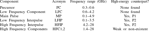
The mean radio profile of the Crab pulsar is complex, with seven distinct components identified so far. The strength of each component depends on frequency: radio observations above
 ${\sim}5~\text{GHz}$
find a very different profile from that seen at lower radio frequencies. We show the radio evolution of the mean profile, with components labelled, in figure 1, and summarize the components in table 2.
${\sim}5~\text{GHz}$
find a very different profile from that seen at lower radio frequencies. We show the radio evolution of the mean profile, with components labelled, in figure 1, and summarize the components in table 2.

Figure 1. Mean radio profiles for the Crab pulsar at a number of frequencies with formal Gaussian fits overplotted. The dominant components discussed in this paper are described in the text and summarized with acronyms in table 2. The Main Pulse (MP) and the two Interpulses (LFIP, HFIP) are coincident in phase with the two peaks in the high-energy profile, which suggests a similar spatial origin for the radio and high-energy emission. The High Frequency Components have not been clearly detected in high-energy profiles. Additional radio components seen at low frequencies, the Precursor (PC) and the Low Frequency Component (LFC), may come from low altitudes close to the star’s polar cap. Nomenclature is from Moffett & Hankins (Reference Moffett and Hankins1996); figure from Hankins et al. (Reference Hankins, Jones and Eilek2015).
The Crab’s mean profile at low radio frequencies – between
 ${\sim}100~\text{MHz}$
and
${\sim}100~\text{MHz}$
and
 ${\sim}5~\text{GHz}$
– is dominated by two peaks, the Main Pulse and the Low Frequency Interpulse, separated by
${\sim}5~\text{GHz}$
– is dominated by two peaks, the Main Pulse and the Low Frequency Interpulse, separated by
 ${\sim}145^{\circ }$
of rotation phase. Both are phase coincident with the two strong peaks in the high-energy light curves (e.g. Abdo et al.
Reference Abdo, Ackerman, Ajello, Atwood, Axelsson, Baldini, Ballet, Barbiellini, Baring and Bastieri2010; Zampieri et al.
Reference Zampieri, Cadez, Barbieri, Naletto, Calvani, Barbieri, Verroi, Zoccarato and Occhipinti2014). However, both radio components are significantly narrower in phase than their high-energy counterparts, and each radio pulse lags the corresponding high-energy pulse by
${\sim}145^{\circ }$
of rotation phase. Both are phase coincident with the two strong peaks in the high-energy light curves (e.g. Abdo et al.
Reference Abdo, Ackerman, Ajello, Atwood, Axelsson, Baldini, Ballet, Barbiellini, Baring and Bastieri2010; Zampieri et al.
Reference Zampieri, Cadez, Barbieri, Naletto, Calvani, Barbieri, Verroi, Zoccarato and Occhipinti2014). However, both radio components are significantly narrower in phase than their high-energy counterparts, and each radio pulse lags the corresponding high-energy pulse by
 ${\sim}2{-}3^{\circ }$
of phase. Two additional weak components can be seen at low radio frequencies: the Precursor leads the Main Pulse by
${\sim}2{-}3^{\circ }$
of phase. Two additional weak components can be seen at low radio frequencies: the Precursor leads the Main Pulse by
 ${\sim}20^{\circ }$
and the Low Frequency Component leads the Main Pulse by
${\sim}20^{\circ }$
and the Low Frequency Component leads the Main Pulse by
 ${\sim}37^{\circ }$
.
${\sim}37^{\circ }$
.
The Crab’s mean profile is quite different at high radio frequencies. It is dominated by an interpulse and two new components which are weak or non-existent below
 ${\sim}5~\text{GHz}$
. The Main Pulse nearly disappears above
${\sim}5~\text{GHz}$
. The Main Pulse nearly disappears above
 ${\sim}8~\text{GHz}$
. The interpulse undergoes a discontinuous phase shift of
${\sim}8~\text{GHz}$
. The interpulse undergoes a discontinuous phase shift of
 ${\sim}7^{\circ }$
, and also undergoes a dramatic change in the spectral and temporal properties of its single pulses. Because the differences between the Low Frequency and High Frequency Interpulses are so striking, we identify them as two separate components. Despite the
${\sim}7^{\circ }$
, and also undergoes a dramatic change in the spectral and temporal properties of its single pulses. Because the differences between the Low Frequency and High Frequency Interpulses are so striking, we identify them as two separate components. Despite the
 $7^{\circ }$
phase shift, the High Frequency Interpulse is also phase coincident with the second of the two broad peaks in the high-energy light curve, but now this radio component leads the high-energy component by
$7^{\circ }$
phase shift, the High Frequency Interpulse is also phase coincident with the second of the two broad peaks in the high-energy light curve, but now this radio component leads the high-energy component by
 ${\sim}3^{\circ }$
of a phase.
${\sim}3^{\circ }$
of a phase.
Two new mean profile components appear at high radio frequencies: the High Frequency Components. These first appear at a few GHz, and become increasingly dominant going to higher frequencies. By 28 GHz, the highest frequency at which we have a mean profile, the two High Frequency Components are as strong as the High Frequency Interpulse. Unlike other components, the High Frequency Components drift in rotation phase, appearing later in phase as one goes to higher frequencies. There is no clear sign of either High Frequency Component in high-energy profiles, except for a weak possible detection in the
 ${\gtrsim}10~\text{GeV}$
profile of Abdo et al. (Reference Abdo, Ackerman, Ajello, Atwood, Axelsson, Baldini, Ballet, Barbiellini, Baring and Bastieri2010).
${\gtrsim}10~\text{GeV}$
profile of Abdo et al. (Reference Abdo, Ackerman, Ajello, Atwood, Axelsson, Baldini, Ballet, Barbiellini, Baring and Bastieri2010).
The fact that we see seven radio components, distributed throughout the full rotation period, immediately tells us we are not seeing low-altitude polar cap emission. If that were the case, we would see at most two components, separated by
 ${\sim}180^{\circ }$
of phase. Furthermore, both the magnetic inclination angle and viewing angle of the pulsar would have to be
${\sim}180^{\circ }$
of phase. Furthermore, both the magnetic inclination angle and viewing angle of the pulsar would have to be
 ${\sim}90^{\circ }$
in order for two polar cap components to be detected. That requirement disagrees with our known viewing angle of
${\sim}90^{\circ }$
in order for two polar cap components to be detected. That requirement disagrees with our known viewing angle of
 ${\sim}60^{\circ }$
relative to the star’s rotation axis (determined from the X-ray torus which surrounds the pulsar; Ng & Romani Reference Ng and Romani2004). We thus conclude – consistent with arguments in § 2.3 – that the main radio pulsesFootnote
6
from the Crab pulsar come from high-altitude regions in the magnetosphere.
${\sim}60^{\circ }$
relative to the star’s rotation axis (determined from the X-ray torus which surrounds the pulsar; Ng & Romani Reference Ng and Romani2004). We thus conclude – consistent with arguments in § 2.3 – that the main radio pulsesFootnote
6
from the Crab pulsar come from high-altitude regions in the magnetosphere.
Table 2. Components of the mean radio profile of the Crab pulsar which we discuss in this paper. The frequency range describes the range over which components have been found in mean profiles from our group (Moffett & Hankins Reference Moffett and Hankins1996; Hankins et al.
Reference Hankins, Jones and Eilek2015) or other work (e.g. Rankin et al.
Reference Rankin, Comella, Craft, Richards, Campbell and Counselman1970). We have occasionally detected single Main Pulses and Low-Frequency Interpulses above the listed frequency ranges, but they are too rare to contribute to mean profiles. Acronyms used are as in figure 1. The two peaks seen in high-energy profiles are P1 (‘main pulse’) and P2 (‘interpulse’); they can be tracked continuously from optical (Słowikowska et al.
Reference Słowikowska, Kanbach, Kramer and Stefanescu2009) to
 ${\it\gamma}$
-rays (e.g. Abdo et al.
Reference Abdo, Ackerman, Ajello, Atwood, Axelsson, Baldini, Ballet, Barbiellini, Baring and Bastieri2010).
${\it\gamma}$
-rays (e.g. Abdo et al.
Reference Abdo, Ackerman, Ajello, Atwood, Axelsson, Baldini, Ballet, Barbiellini, Baring and Bastieri2010).
4.2 Our single-pulse observations of the Crab pulsar
Our main focus in this paper is what we have learned about individual Main Pulses and interpulses from our high-time-resolution observations of the Crab pulsar. This work was carried out at between 1993 and 1999 at the Karl G. Jansky Very Large Array, between 2002 and 2009 at the Arecibo Observatory and from 2009 and 2011 at the Robert C. Byrd Green Bank Telescope. Details of our single-pulse observations and data acquisition system are given in Hankins & Eilek (Reference Hankins and Eilek2007) and Hankins et al. (Reference Hankins, Jones and Eilek2015). Our net ‘take’ was 1440 bright single pulses above
 ${\sim}1~\text{GHz}$
with high enough signal-to-noise to be useful. Pulses at lower frequencies are significantly broadened by interstellar scintillation, thus not useful for our analysis here. We captured approximately 870 strong Main Pulses, 540 strong interpulses (510 of which were High Frequency Interpulses, the rest Low Frequency Interpulses) and 30 High Frequency Component pulses. In this paper we focus on the Main Pulse and the two interpulses, for which our data allow useful comparisons to the models.
${\sim}1~\text{GHz}$
with high enough signal-to-noise to be useful. Pulses at lower frequencies are significantly broadened by interstellar scintillation, thus not useful for our analysis here. We captured approximately 870 strong Main Pulses, 540 strong interpulses (510 of which were High Frequency Interpulses, the rest Low Frequency Interpulses) and 30 High Frequency Component pulses. In this paper we focus on the Main Pulse and the two interpulses, for which our data allow useful comparisons to the models.
Because our data acquisition system is triggered only by the brightest pulses, we have captured single pulses from the bright end of the pulse fluence distribution. These are sometimes called ‘giant pulses’ in the literature. However, there is no evidence that these are any different from fainter, ‘normal’ pulses that make up the majority of the star’s pulsed radio emission. We therefore assume the pulses we have captured are good representatives of the emission physics for both high and low radio power.
Our single-pulse work shows that two very different types of radio emission physics exist in the magnetosphere of the Crab pulsar. As we show in the following sections, single Main Pulses and Low Frequency Interpulses share the same temporal and spectral characteristics, while single High Frequency Interpulses are very different. This result was totally unexpected. In § 2 we argued that the Main Pulse and the two Interpulses should be associated with the star’s two magnetic poles, probably from high-altitude caustics above each pole. However, because no pulsar model to date predicts any asymmetry between the north and south magnetic poles, there is no reason to expect the radio emission physics from the two regions to be different. And yet that seems to be the case.
We emphasize that we have not seen any secular changes in the properties of the Main Pulse or either Interpulse. The characteristics we summarize here are robust and constant, over the nearly 20 years we have observed this pulsar. In the rest of this paper we present the detailed characteristics of each type of radio component, and consider how well – if at all – existing models can explain the observations.
5 Main Pulse emission: microbursts and nanoshots
Although the Main Pulse and Low Frequency Interpulse components of the mean profile are smooth and well fit by Gaussians (as in figure 1), the story is very different when pulses are observed individually.
5.1 Explosive bursts of radio emission
The radio emission in a single Main Pulse or Low Frequency Interpulse comes in microbursts: abrupt releases of coherent radio emission with a characteristic time of a few microseconds. Figure 2 shows two such examples. These bursts can occur anywhere in the probability envelope defined by the mean profile component, which extends for several hundred microseconds (figure 1). The burst strength is highly variable. The strongest bursts are the most dramatic, but weak bursts are more common. Furthermore, detectable bursts occur in random groups that persist for a few minutes, between longer periods of radio silence.
The spectrum of a microburst is relatively broadband. As figure 2 shows, it fills our observing bandwidth, which was typically 2 or 4 GHz for most of our observations, and extended to 8 GHz for one data set. No lower frequency limit has been found for Main Pulse emission; that component can be seen in mean profiles well below 100 MHz (e.g. Rankin et al.
Reference Rankin, Comella, Craft, Richards, Campbell and Counselman1970). Main Pulses and Low Frequency Interpulses become faint and/or scarce above
 ${\sim}10~\text{GHz}$
. They disappear from mean profiles and we have captured very few single pulses in these phase windows at higher frequencies.
${\sim}10~\text{GHz}$
. They disappear from mean profiles and we have captured very few single pulses in these phase windows at higher frequencies.
5.2 Sporadic energy release in the emission zone
Microbursts show that the radio emission region is neither uniform nor homogeneous. It must be highly variable in space and time, producing the short-lived bursts of radio emission from isolated regions within the emission zone. We therefore need some process which sporadically creates localized regions in which conditions are conducive to coherent radio emission. We do not know the radio emission mechanism, but nearly all models rely on a relativistic particle beam (as we discuss in § 6 and appendix A). The sporadic nature of the radio bursts tells us that the driving beams are not steady. They must dissipate after their energy is given up to the radio emission and be continually regenerated throughout the emission region.

Figure 2. Two typical examples of Main Pulses. (a,b) Show intensity integrated across our observing band. The radio emission comes in distinct bursts, each lasting less than a microsecond. (c,d) Show the dynamic spectrum within our observing band; the orange line on the left shows the equalized frequency response of the receiver. The spectrum of each microburst is relatively broadband, spanning the full observing bandwidth (but compare the pulse shown in figure 3, where individual, narrowband shots within the pulse can be resolved). Data were obtained with time resolution equal to the inverse of the observing bandwidth. For display purposes, both pulses have been smoothed to time resolution 51.2 ns and spectral resolution 78 MHz. Both pulses were dedispersed with DM
 $56.73762~\text{pc}~\text{cm}^{-3}$
(see § 8.1 for definition of DM).
$56.73762~\text{pc}~\text{cm}^{-3}$
(see § 8.1 for definition of DM).
The driving beams must themselves be driven by electric fields. In highly magnetized regions such as the pulsar magnetosphere, the driving
 $\boldsymbol{E}$
must be parallel to the local
$\boldsymbol{E}$
must be parallel to the local
 $\boldsymbol{B}$
. Thus,
$\boldsymbol{B}$
. Thus,
 $E_{\Vert }$
must itself be sporadic: reaching high strengths, creating the particle beam, then – perhaps – being shorted out. This picture was originally suggested for the polar cap by Ruderman & Sutherland (Reference Ruderman and Sutherland1975), and has been explored numerically by Levinson et al. (Reference Levinson, Melrose, Judge and Luo2005) and Timokhin & Arons (Reference Timokhin and Arons2013). Their simulations verify that cyclic behaviour can be a direct consequence of low-altitude magnetic pair production, as follows. Say we start with a finite
$E_{\Vert }$
must itself be sporadic: reaching high strengths, creating the particle beam, then – perhaps – being shorted out. This picture was originally suggested for the polar cap by Ruderman & Sutherland (Reference Ruderman and Sutherland1975), and has been explored numerically by Levinson et al. (Reference Levinson, Melrose, Judge and Luo2005) and Timokhin & Arons (Reference Timokhin and Arons2013). Their simulations verify that cyclic behaviour can be a direct consequence of low-altitude magnetic pair production, as follows. Say we start with a finite
 $E_{\Vert }$
driven by the star’s rotation in a nearly empty gap region. It accelerates charges, which in turn create
$E_{\Vert }$
driven by the star’s rotation in a nearly empty gap region. It accelerates charges, which in turn create
 ${\it\gamma}$
-rays by curvature radiation. The
${\it\gamma}$
-rays by curvature radiation. The
 ${\it\gamma}$
-ray photons decay into
${\it\gamma}$
-ray photons decay into
 $e^{+}e^{-}$
pairs, which fill the gap region and shield
$e^{+}e^{-}$
pairs, which fill the gap region and shield
 $E_{\Vert }$
. Once the electric field is neutralized, particle acceleration ceases, the existing pairs stream out of the region and the original
$E_{\Vert }$
. Once the electric field is neutralized, particle acceleration ceases, the existing pairs stream out of the region and the original
 $E_{\Vert }$
is recovered as the gap again becomes (nearly) empty.
$E_{\Vert }$
is recovered as the gap again becomes (nearly) empty.
The radio microbursts tell us that a similar process is needed in the high-altitude radio emission regions of the Crab pulsar. However, the magnetic field is too low in those regions for magnetic pair production to take place in situ. It may be that the particle beams which drive the radio emission have propagated from their natal regions above the polar caps, but it is not obvious that they would retain their identity and still have the sporadic and inhomogeneous nature required to explain the microbursts. Alternatively, two-photon pair creation may take place within the high-altitude gaps (e.g. Ho Reference Ho1989; Cheng, Ruderman & Zhang Reference Cheng, Ruderman and Zhang2000). The seed
 ${\it\gamma}$
-rays are still thought to come from curvature radiation of charges accelerated by unshielded
${\it\gamma}$
-rays are still thought to come from curvature radiation of charges accelerated by unshielded
 $E_{\Vert }$
fields. The target photons (likely X-rays) may be thermal emission from the star’s surface, or secondary photons from a low-altitude pair cascade. While this process has not been studied in detail, it seems likely that an oscillatory
$E_{\Vert }$
fields. The target photons (likely X-rays) may be thermal emission from the star’s surface, or secondary photons from a low-altitude pair cascade. While this process has not been studied in detail, it seems likely that an oscillatory
 $E_{\Vert }$
cycle can also be characteristic of high-altitude gap regions.
$E_{\Vert }$
cycle can also be characteristic of high-altitude gap regions.

Figure 3. An example of nanoshots in a Main Pulse. (a,c) Shows the total intensity and dynamic spectrum, dedispersed with DM
 $56.76378~\text{pc}~\text{cm}^{-3}$
; layout is the same as in figure 2. The radio emission in this pulse is confined to a set of well-separated nanoshots. Each nanoshot lasts of the order of a nanosecond and is relatively narrowband (frequency spread
$56.76378~\text{pc}~\text{cm}^{-3}$
; layout is the same as in figure 2. The radio emission in this pulse is confined to a set of well-separated nanoshots. Each nanoshot lasts of the order of a nanosecond and is relatively narrowband (frequency spread
 ${\it\delta}{\it\nu}\sim 0.1{\it\nu}$
). Shown with time resolution 51.2 ns and spectral resolution 39.1 MHz. (b,d) is a zoom into the nanoshots seen between 18 and
${\it\delta}{\it\nu}\sim 0.1{\it\nu}$
). Shown with time resolution 51.2 ns and spectral resolution 39.1 MHz. (b,d) is a zoom into the nanoshots seen between 18 and
 $27~{\rm\mu}\text{s}$
in (a,c), now displayed at 4 ns time resolution. At this resolution, individual nanoshots within the clump at
$27~{\rm\mu}\text{s}$
in (a,c), now displayed at 4 ns time resolution. At this resolution, individual nanoshots within the clump at
 $24~{\rm\mu}\text{s}$
are now resolved. The different time smoothing in this view gives different peak fluxes for each nanoshot. (b) shows the total intensity (I; black), linearly polarized intensity (L; green) and circularly polarized intensity (V; red). (d) shows the position angle of the linear polarization. Only polarized flux above 4 times the off-pulse noise (indicated by the orange lines in b) is shown. Note the strong circular polarization of individual nanoshots can be of either sign.
$24~{\rm\mu}\text{s}$
are now resolved. The different time smoothing in this view gives different peak fluxes for each nanoshot. (b) shows the total intensity (I; black), linearly polarized intensity (L; green) and circularly polarized intensity (V; red). (d) shows the position angle of the linear polarization. Only polarized flux above 4 times the off-pulse noise (indicated by the orange lines in b) is shown. Note the strong circular polarization of individual nanoshots can be of either sign.
5.3 Nanoshots
Once in a while, a Main Pulse or a Low Frequency Interpulse can be resolved into very brief nanoshots. We show examples in figure 3; others can be seen in Hankins et al. (Reference Hankins, Eilek and Jones2016). Because we believe these nanoshots provide a critical test of the radio emission mechanism, we highlight their properties here.
Time scales. Some of the nanoshots we have captured are unresolved at our best time resolution (a fraction of a nanosecond; the inverse of our observing bandwidth). Others are marginally resolved, lasting of the order of a nanosecond. The example pulse we show in figure 3 is substantially smoothed, for clarity of presentation. Nanoshots displayed at higher time resolution can be found in Hankins et al. (Reference Hankins, Kern, Weatherall and Eilek2003) and Hankins & Eilek (Reference Hankins and Eilek2007).
Spectrum. Each isolated nanoshot we have captured is relatively narrowband, with fractional bandwidth
 ${\it\delta}{\it\nu}/{\it\nu}$
of the order of 10 %. Figure 3 shows that the centre frequency of the nanoshots is not fixed, but can be anywhere within our observing band. The product of the centre frequency,
${\it\delta}{\it\nu}/{\it\nu}$
of the order of 10 %. Figure 3 shows that the centre frequency of the nanoshots is not fixed, but can be anywhere within our observing band. The product of the centre frequency,
 ${\it\nu}_{obs}$
, and duration,
${\it\nu}_{obs}$
, and duration,
 ${\it\delta}t$
, of a nanoshot turns out to be a useful diagnostic for the models. For each isolated nanoshot we have captured between 5 and 10 GHz this product
${\it\delta}t$
, of a nanoshot turns out to be a useful diagnostic for the models. For each isolated nanoshot we have captured between 5 and 10 GHz this product
 ${\it\nu}_{obs}{\it\delta}t\sim O(10)$
.
${\it\nu}_{obs}{\it\delta}t\sim O(10)$
.
Polarization. As the example in figure 3 shows, individual nanoshots tend to be elliptically polarized. While most of them show some linear polarization, they are often dominated by circular polarization (CP). The sign of the CP can change from one nanoshot to the next, apparently at random.
Although microbursts in most Main Pulses and Low Frequency Interpulses last longer and have a broader dynamic spectrum than do the nanoshots, we suspect that microbursts are incoherent superpositions of short-lived narrowband, nanoshots. In other words, all microbursts are ‘clumps of nanoshots’. This is supported by the observationally motivated amplitude-modulated noise model of pulsar emission (Rickett Reference Rickett1975). Because each such microburst is broadband (§ 5.1), the centre frequencies of the nanoshots within a microburst must span a wide frequency range.
6 Nanoshots as tests of radio emission models
It has been hard, historically, to compare radio emission models to the data. The models address physical processes on plasma microscales, but most of the data can only address larger-scale, system-wide processes. We believe the nanoshots in the Main Pulse and Low Frequency Interpulse, revealed by our very high-time-resolution observations, provide a key clue to the underlying physics.
In this section we use our data to confront three plausible models from appendix A. Because each model can be connected to the spectrum, duration and/or polarization of an individual nanoshot, we can constrain physical conditions which must hold in the radio emission region in order for that model to work.
For easy reference in the following discussion we refer back to the basic magnetospheric parameters of the Crab pulsar in table 1. We highlight the three models in table 3 and summarize the plasma conditions required by each model in table 4.
6.1 Strong plasma turbulence
When electrostatic turbulence is driven to large amplitude (which we call ‘strong plasma turbulence’, SPT), a modulational instability creates localized Langmuir wave solitons. These solitons are themselves unstable, generating electromagnetic waves which can escape the plasma, and potentially be observed as nanoshots. We generally follow Weatherall (Reference Weatherall1997, Reference Weatherall1998); see also § A.1.
Spectrum. Individual bursts are emitted around the plasma frequency in the comoving plasma frame. If the plasma is moving out from the pulsar at a streaming speed
 ${\it\gamma}_{s}$
, we observe nanoshots centred at
${\it\gamma}_{s}$
, we observe nanoshots centred at
 $$\begin{eqnarray}\displaystyle {\it\nu}_{obs}^{SPT}\sim 2{\it\gamma}_{s}^{1/2}{\it\nu}_{p}, & & \displaystyle\end{eqnarray}$$
where
 ${\it\nu}_{p}$
is the plasma frequency, and everything is written in the observer’s frame. Conditions required to put
${\it\nu}_{p}$
is the plasma frequency, and everything is written in the observer’s frame. Conditions required to put
 ${\it\nu}_{obs}$
in the radio band are given in table 4 and § 6.4. Simulations by Weatherall (Reference Weatherall1998) predict the nanoshots will be relatively narrowband, with
${\it\nu}_{obs}$
in the radio band are given in table 4 and § 6.4. Simulations by Weatherall (Reference Weatherall1998) predict the nanoshots will be relatively narrowband, with
 ${\it\delta}{\it\nu}/{\it\nu}_{obs}\sim {\it\Lambda}$
, where
${\it\delta}{\it\nu}/{\it\nu}_{obs}\sim {\it\Lambda}$
, where
 ${\it\Lambda}$
measures the strength of the turbulence. Using
${\it\Lambda}$
measures the strength of the turbulence. Using
 ${\it\Lambda}\gtrsim 0.1$
, from Weatherall (Reference Weatherall1997, Reference Weatherall1998), this prediction agrees with our observations of isolated nanoshots (§ 5.3).
${\it\Lambda}\gtrsim 0.1$
, from Weatherall (Reference Weatherall1997, Reference Weatherall1998), this prediction agrees with our observations of isolated nanoshots (§ 5.3).
Time scales. The dynamic time scale for soliton collapse, and the duration of the consequent flare of radiation, is
 ${\it\delta}t\sim 1/(2{\it\gamma}_{s}^{1/2}{\it\Lambda}{\it\nu}_{p})$
, again written in the observer’s frame. Using (6.1), this model predicts that radiation bursts observed at a few GHz last of the order of a nanosecond, and have the product
${\it\delta}t\sim 1/(2{\it\gamma}_{s}^{1/2}{\it\Lambda}{\it\nu}_{p})$
, again written in the observer’s frame. Using (6.1), this model predicts that radiation bursts observed at a few GHz last of the order of a nanosecond, and have the product
 ${\it\nu}_{obs}{\it\delta}t\sim 1/{\it\Lambda}$
. These predictions are also consistent with our observations of isolated nanoshots.
${\it\nu}_{obs}{\it\delta}t\sim 1/{\it\Lambda}$
. These predictions are also consistent with our observations of isolated nanoshots.
Polarization. The collapsing soliton generates electromagnetic waves whose polarization is set by local plasma conditions. Weatherall (Reference Weatherall1998) worked in the context of a strongly magnetized plasma, in which charges can only move along the magnetic field. In this limit, emergent radiation around the plasma frequency is linearly polarized along the magnetic field. Because nanoshots from the Crab pulsar can show strong circular polarization, they cannot be explained by Weatherall’s model as it stands. That model would have to be extended, perhaps to a plasma in which the natural modes are elliptically polarized.
Table 3. Overview of nanoshot models discussed in the text.

a Both SPT and FEM, as currently formulated, predict fully linear polarization, which disagrees with the observations.
b The densities needed for CIE to match observations are much higher than magnetosphere theories predict.
c The current formulation of CIE cannot address the short-lived nanoshots we observe.
Table 4. Plasma conditions required for radio emission models discussed in § 6 to match the spectrum of the nanoshots. The density of the pair plasma is
 $n$
; for comparison, table 1 shows the GJ density
$n$
; for comparison, table 1 shows the GJ density
 $n_{GJ}\sim (2\times 10^{6}-2\times 10^{7})~\text{cm}^{-3}$
in the upper magnetosphere. The Lorentz factor
$n_{GJ}\sim (2\times 10^{6}-2\times 10^{7})~\text{cm}^{-3}$
in the upper magnetosphere. The Lorentz factor
 ${\it\gamma}_{s}$
describes the streaming speed of the pair plasma;
${\it\gamma}_{s}$
describes the streaming speed of the pair plasma;
 ${\it\gamma}_{b}$
describes the speed of the particle beam that drives FEM emission, which must satisfy
${\it\gamma}_{b}$
describes the speed of the particle beam that drives FEM emission, which must satisfy
 ${\it\gamma}_{b}^{2}\sim O(10)$
to match the observations;
${\it\gamma}_{b}^{2}\sim O(10)$
to match the observations;
 ${\it\gamma}_{res}$
describes the energy of the beam particles which participate in the cyclotron resonance. The magnetic field is scaled to
${\it\gamma}_{res}$
describes the energy of the beam particles which participate in the cyclotron resonance. The magnetic field is scaled to
 $10^{6}~\text{G}$
, the smallest field likely within the standard picture of the magnetosphere.
$10^{6}~\text{G}$
, the smallest field likely within the standard picture of the magnetosphere.
6.2 Free-electron maser emission
A relativistic electron beam, moving parallel to the magnetic field, generates Langmuir turbulence as usual. The interaction of the beam particles with that turbulence leads to coherent bunching of the beam charges, and consequent strong bursts of radiation. This model is similar to the SPT model, but here the beam itself is what radiates; emission from the background plasma is not considered. See also § A.2.
Spectrum. Bunched electron beams, moving at
 ${\it\gamma}_{b}$
, scatter on intense, localized electrostatic waves of the plasma turbulence. The scattered radiation can be treated as inverse Compton scattering of the Langmuir photons. If the plasma is at rest, the scattered photon frequency isFootnote
7
${\it\gamma}_{b}$
, scatter on intense, localized electrostatic waves of the plasma turbulence. The scattered radiation can be treated as inverse Compton scattering of the Langmuir photons. If the plasma is at rest, the scattered photon frequency isFootnote
7
 $$\begin{eqnarray}\displaystyle {\it\nu}_{obs}^{FEM}\sim 2{\it\gamma}_{b}^{2}{\it\nu}_{p} & & \displaystyle\end{eqnarray}$$
(e.g. Benford Reference Benford1992). Conditions required to put
 ${\it\nu}_{obs}$
in the radio band are given in table 4 and § 6.4.
${\it\nu}_{obs}$
in the radio band are given in table 4 and § 6.4.
Time scales. Short-lived radiation bursts arise naturally in a free-electron maser, when the beam particles interact with electric fields in the Langmuir turbulence they have generated. Both the coherent charge bunching, and the consequent radiation bursts, are characterized by the plasma time scale for the background plasma:
 ${\it\delta}t\sim 1/{\it\nu}_{p}$
(e.g. Schopper et al.
Reference Schopper, Ruhl, Kunzl and Lesch2003). Thus, this model predicts the product
${\it\delta}t\sim 1/{\it\nu}_{p}$
(e.g. Schopper et al.
Reference Schopper, Ruhl, Kunzl and Lesch2003). Thus, this model predicts the product
 ${\it\nu}_{obs}{\it\delta}t\sim {\it\gamma}_{b}^{2}$
. Clearly the beam cannot be too fast;
${\it\nu}_{obs}{\it\delta}t\sim {\it\gamma}_{b}^{2}$
. Clearly the beam cannot be too fast;
 ${\it\gamma}_{b}^{2}\sim O(10)$
is needed to match the frequency-duration product of our observed nanoshots.
${\it\gamma}_{b}^{2}\sim O(10)$
is needed to match the frequency-duration product of our observed nanoshots.
Polarization. Both the oscillating electric field in the induced Langmuir turbulence, and the motion of beam charges in that field, are parallel to the local magnetic field. It follows that radiation bursts are linearly polarized, also parallel to
 $\boldsymbol{B}$
(e.g. Windsor & Kellog Reference Windsor and Kellog1974). This model would also have to be extended to accommodate circular polarization. Perhaps the bunched beam charges have finite and synchronized pitch angles. This can work in the lab; Benford & Tzach (Reference Benford and Tzach2000) reported coherent synchrotron emission from bunched electrons in an incoming rotating beam. However, it is not clear that such a situation would arise naturally in a pulsar magnetosphere.
$\boldsymbol{B}$
(e.g. Windsor & Kellog Reference Windsor and Kellog1974). This model would also have to be extended to accommodate circular polarization. Perhaps the bunched beam charges have finite and synchronized pitch angles. This can work in the lab; Benford & Tzach (Reference Benford and Tzach2000) reported coherent synchrotron emission from bunched electrons in an incoming rotating beam. However, it is not clear that such a situation would arise naturally in a pulsar magnetosphere.
6.3 Cyclotron instability emission
A relativistic particle beam moving into a magnetized plasma generates transverse waves when it couples to the plasma through the anomalous cyclotron resonance. Because the waves can escape the plasma without mode conversion, this is a direct emission process. This theory has been applied to pulsars by Kazbegi, Machabeli & Melikidze (Reference Kazbegi, Machabeli and Melikidze1991, ‘K91’) and Lyutikov, Machabeli & Blandford (Reference Lyutikov, Machabeli and Blandford1999, ‘L99’, and references therein). To compare this model to Main Pulse nanoshots, we follow the specific problem set-up assumed by those authors: one-dimensional motion of a cold pair plasma, streaming outward from the pulsar at
 ${\it\gamma}_{s}$
, as well as a faster ‘primary beam’ moving through that plasma at
${\it\gamma}_{s}$
, as well as a faster ‘primary beam’ moving through that plasma at
 ${\it\gamma}_{b}$
. See also § A.3.
${\it\gamma}_{b}$
. See also § A.3.
Spectrum. Emission proceeds through the first harmonic of the anomalous cyclotron resonance. The escaping radiation is around the resonant frequency:
 $$\begin{eqnarray}\displaystyle {\it\nu}_{obs}^{CIE}={\it\nu}_{B}\frac{4{\it\nu}_{B}^{2}}{{\it\nu}_{p}^{2}}\frac{{\it\gamma}_{s}^{3}}{{\it\gamma}_{res}}, & & \displaystyle\end{eqnarray}$$
where
 ${\it\nu}_{B}$
is the electron cyclotron frequency and
${\it\nu}_{B}$
is the electron cyclotron frequency and
 ${\it\gamma}_{res}$
is the Lorentz factor of the resonant beam particles (
${\it\gamma}_{res}$
is the Lorentz factor of the resonant beam particles (
 ${\it\gamma}_{s}<{\it\gamma}_{res}<{\it\gamma}_{b}$
). All terms are written in the observer’s frame, and the solution describes waves propagating nearly along the magnetic field. Because this is a resonant process, operating at the lowest harmonic, we guess the emission is relatively narrowband. Conditions required to put
${\it\gamma}_{s}<{\it\gamma}_{res}<{\it\gamma}_{b}$
). All terms are written in the observer’s frame, and the solution describes waves propagating nearly along the magnetic field. Because this is a resonant process, operating at the lowest harmonic, we guess the emission is relatively narrowband. Conditions required to put
 ${\it\nu}_{obs}$
in the radio band are given in table 4 and § 6.4.
${\it\nu}_{obs}$
in the radio band are given in table 4 and § 6.4.
Time scales. Because this model has not been carried past the linear instability calculation, it cannot address short-lived nanoshots. One would expect the instability to generate resonant plasma waves, some remaining in the plasma to generate pitch-angle scattering, others potentially escaping to be seen as radio emission. Lyutikov considered possible saturation mechanisms (e.g. L99 & references therein), but did not discuss self-generated coherent particle bunching, which would be needed for bright radio nanoshots.
Polarization. If the distribution functions of the electrons and positrons in a pair plasma are different, the normal modes of the plasma become circularly polarized for propagation close to the magnetic field (Allen & Melrose Reference Allen and Melrose1982, K91). The CIE models of K91/L99 take advantage of this fact by assuming relative streaming between the two species. If the electrons are moving faster than the positrons, their model predicts left-handed CP; if the positrons are moving faster, one gets right-handed CP.
6.4 Nanoshots: implications for the emission region
In this section we have compared three beam-driven radio emission models to our nanoshot data. Each model has its own requirements on the plasma density in the emission region, which we summarize here and in table 4. We also point out that each model requires further development before it can match all of the observations.
6.4.1 SPT and FEM models
Both of these models involve plasma turbulence driven by a relativistic particle beam, presumably via a two-stream instability. The SPT model emphasizes radio emission from collapsing solitons when the turbulence has become strong. The FEM model emphasizes radio emission from coherent charge bunching caused by the beam responding to the turbulence it has created.
In both models the emission frequency is related to the plasma frequency in the background plasma: one boosted by
 ${\it\gamma}_{s}$
, the other by
${\it\gamma}_{s}$
, the other by
 ${\it\gamma}_{b}^{4}$
. In practice, of course, we expect both phenomena to contribute to the nanoshots. The relative importance of the two effects depends on the relative densities of the driving beam and the background plasma, neither of which we attempt to estimate.
${\it\gamma}_{b}^{4}$
. In practice, of course, we expect both phenomena to contribute to the nanoshots. The relative importance of the two effects depends on the relative densities of the driving beam and the background plasma, neither of which we attempt to estimate.
To radiate between 100 MHz and 10 GHz, the emitting plasma density and streaming or beam speeds must satisfy
 $$\begin{eqnarray}\displaystyle n{\it\gamma}_{s}\sim (3\times 10^{7}-3\times 10^{11})~\text{cm}^{-3}\quad \text{or}\quad n{\it\gamma}_{b}^{4}\sim (3\times 10^{7}-3\times 10^{11})~\text{cm}^{-3}\qquad & & \displaystyle\end{eqnarray}$$
for SPT or FEM, respectively. Recalling that
 ${\it\gamma}_{b}^{2}\sim O(10)$
is needed to match the frequency-duration product of the nanoshots, and that
${\it\gamma}_{b}^{2}\sim O(10)$
is needed to match the frequency-duration product of the nanoshots, and that
 ${\it\gamma}_{s}$
may be as low as
${\it\gamma}_{s}$
may be as low as
 ${\sim}10^{2}$
in some models, we see that these two constraints are not dissimilar.
${\sim}10^{2}$
in some models, we see that these two constraints are not dissimilar.
Comparing these constraints to the GJ density in the upper magnetosphere (table 1), we see that the density enhancement,
 ${\it\lambda}=n/n_{GJ}$
, must be in the range given by
${\it\lambda}=n/n_{GJ}$
, must be in the range given by
 $10^{2}\lesssim {\it\lambda}{\it\gamma}_{s}\lesssim 10^{5}$
and/or
$10^{2}\lesssim {\it\lambda}{\it\gamma}_{s}\lesssim 10^{5}$
and/or
 $10^{2}\lesssim {\it\lambda}{\it\gamma}_{b}^{4}\lesssim 10^{5}$
in the emitting region. For modest values of
$10^{2}\lesssim {\it\lambda}{\it\gamma}_{b}^{4}\lesssim 10^{5}$
in the emitting region. For modest values of
 ${\it\gamma}_{s}$
and
${\it\gamma}_{s}$
and
 ${\it\gamma}_{b}$
, the upper part of the required density (or
${\it\gamma}_{b}$
, the upper part of the required density (or
 ${\it\lambda}$
) range is generally consistent with models of pair production close to the polar cap (as in § 2.1). Perhaps pair cascades operating in high-altitude gaps result in similar enhancements and streaming speeds.
${\it\lambda}$
) range is generally consistent with models of pair production close to the polar cap (as in § 2.1). Perhaps pair cascades operating in high-altitude gaps result in similar enhancements and streaming speeds.
The lower end of the density range is problematic, however. Previous authors (e.g. Kunzl et al.
Reference Kunzl, Lesch, Jessner and von Hoensbroech1998; Melrose & Gedalin Reference Melrose and Gedalin1999) have argued that models based on relativistic plasma emission have difficulty explaining radio emission from young pulsars. If the radio emission comes from low altitudes – over the polar cap – the GJ density there is too high, even with
 ${\it\lambda}\sim 1$
, to be compatible with low radio frequencies. This problem is mitigated if the radio emission comes from higher altitudes, as it does in the Crab pulsar. Perhaps the lowest radio frequencies come from high-altitude regions where the plasma density is not significantly enhanced over the GJ density.
${\it\lambda}\sim 1$
, to be compatible with low radio frequencies. This problem is mitigated if the radio emission comes from higher altitudes, as it does in the Crab pulsar. Perhaps the lowest radio frequencies come from high-altitude regions where the plasma density is not significantly enhanced over the GJ density.
6.4.2 CIE model
This model is also beam driven, but the emission proceeds through the cyclotron resonance, which becomes unstable in the low magnetic fields found at high altitudes (for the specific model of K91/L99). Because this model includes relative streaming between electrons and positrons, it can explain the circular polarization we observe in the nanoshots.
Stringent conditions, however are required if this model is to explain the radio data. Matching the resonant frequency (6.3) to the radio band requires
 $$\begin{eqnarray}\displaystyle (n{\it\gamma}_{res}/B^{3}{\it\gamma}_{s}^{2})\sim (1\times 10^{40}-1\times 10^{42})~\text{cm}^{-3}~\text{G}^{-3}. & & \displaystyle\end{eqnarray}$$
Even taking the most optimistic parameter choices within the standard model (
 $B\sim 10^{6}$
G,
$B\sim 10^{6}$
G,
 ${\it\gamma}_{res}\sim 10^{6}$
and
${\it\gamma}_{res}\sim 10^{6}$
and
 ${\it\gamma}_{s}$
of order unity), we still need
${\it\gamma}_{s}$
of order unity), we still need
 $n\sim 10^{16}{-}10^{18}~\text{cm}^{-3}$
in order for this model to produce radio emission.
$n\sim 10^{16}{-}10^{18}~\text{cm}^{-3}$
in order for this model to produce radio emission.
Such high densities require huge pair enhancements,
 ${\it\lambda}\sim 10^{9}{-}10^{11}$
, much higher than predicted by models of polar cap pair cascades (§ 2.1). For comparison, models of the Crab Nebula suggest the mean outflow density from the pulsar exceeds the GJ value by 5 or 6 orders of magnitude (e.g. Bucciantini, Arons & Amato Reference Bucciantini, Arons and Amato2010). While that range also exceeds the
${\it\lambda}\sim 10^{9}{-}10^{11}$
, much higher than predicted by models of polar cap pair cascades (§ 2.1). For comparison, models of the Crab Nebula suggest the mean outflow density from the pulsar exceeds the GJ value by 5 or 6 orders of magnitude (e.g. Bucciantini, Arons & Amato Reference Bucciantini, Arons and Amato2010). While that range also exceeds the
 ${\it\lambda}$
values predicted by pair cascade models, the density enhancement required if the CIE model is to match observations is higher still. Perhaps some process, such as magnetic reconnection, can dump large amounts of mass into high-altitude emission regions. Perhaps unusually low magnetic fields – which would lower the necessary density range – exist in such regions.
${\it\lambda}$
values predicted by pair cascade models, the density enhancement required if the CIE model is to match observations is higher still. Perhaps some process, such as magnetic reconnection, can dump large amounts of mass into high-altitude emission regions. Perhaps unusually low magnetic fields – which would lower the necessary density range – exist in such regions.
6.4.3 What is missing?
None of the three models, as currently formulated, can address all of the data. The SPT and FEM models can explain the existence of the nanoshots, but not their polarization. The CIE model can explain the circularly polarized emission, but cannot explain the existence of the nanoshots.
We suspect the way forward is a combination of the two approaches. If the electrons and positrons have different distributions – for instance, different streaming speeds – the fundamental modes of the plasma are circularly polarized. Alternating signs of CP in different nanoshots require alternating dominance of one or the other species in each nanoshot. Perhaps that can exist in a highly turbulent pair cascade zone. Nanosecond long bursts of coherent radio emission suggest that the emitting charges are coherently bunched. Perhaps that can come from the nonlinear evolution of one or both of these models, operating in a plasma which can carry circular polarization.
7 The High Frequency Interpulse: a different picture
When we first studied individual High Frequency Interpulses, in 2004–2006, we were astonished to find they have very different properties from Main Pulses and Low Frequency Interpulses. Since then we have continued to study them, over several years, going to other telescopes and higher radio frequencies. The result is unchanged: High Frequency Interpulses are very different from Main Pulses and Low Frequency Interpulses, in ways no current model of pulsar radio emission can explain.
7.1 Microbursts but no nanoshots
The temporal signature of High Frequency Interpulses is similar to that of Main Pulses and Low Frequency Interpulses (§ 5), but with important differences. Single High Frequency Interpulses typically contain two or three microbursts, each lasting a few microseconds and overlapping in time. Figure 4 shows two examples. As with Main Pulses and Low Frequency Interpulses, individual High Frequency Interpulses are much shorter lived than the corresponding component in the pulsar’s mean profile. Single pulses can occur anywhere within the mean profile envelope; more than one pulse, typically separated by a few hundred
 ${\rm\mu}\text{s}$
, can occur in the same rotation period.
${\rm\mu}\text{s}$
, can occur in the same rotation period.
Also as with the Main Pulse and Low Frequency Interpulse, the emission region for the High Frequency Interpulse is dynamic. Localized hot spots, with conditions favourable to radio emission, are created intermittently throughout the broad emission region. Each hot spot emits a burst of coherent radio emission, then dies away, in only a few
 ${\rm\mu}\text{s}$
. Similar hot spots are regenerated again and again throughout the extended emission region that is the source of the High Frequency Interpulse.
${\rm\mu}\text{s}$
. Similar hot spots are regenerated again and again throughout the extended emission region that is the source of the High Frequency Interpulse.
There are, however, some differences between the time signature of High Frequency Interpulses, and that of Main Pulses and Low Frequency Interpulses. Each microburst in a High-Frequency Interpulse lasts approximately ten times longer than that in a Main Pulse (compare figures 2 and 4). We have never recorded a High Frequency Interpulse with the well-separated, sub-
 ${\rm\mu}\text{s}$
bursts that characterize the Main Pulses, nor have we ever captured isolated nanoshots in a High Frequency Interpulse. These details suggest to us that the energy storage/release mechanism – be it particle beams driven by
${\rm\mu}\text{s}$
bursts that characterize the Main Pulses, nor have we ever captured isolated nanoshots in a High Frequency Interpulse. These details suggest to us that the energy storage/release mechanism – be it particle beams driven by
 $E_{\Vert }$
, or something completely different – is not the same in the two types of emission regions.
$E_{\Vert }$
, or something completely different – is not the same in the two types of emission regions.

Figure 4. Two typical examples of High Frequency Interpulses, shown with the same layout as in figure 2. Each pulse contains a small number of bursts, each one lasting a few microseconds. Comparison to figure 2 shows that bursts in this component are fewer, and longer lived, than in a typical main pulse. The dynamic spectra show the radio emission is concentrated in narrow spectral emission bands. These bands are very different from the Main Pulse spectra (figures 2 and 3), and were not predicted by any model of pulsar radio emission. Each microburst in a High Frequency Interpulse has its own band sets: four sets can be seen in the pulse in (a,c), and (probably) three can be found in the pulse in (b,d). Pulse in (a,c) was dedispersed with DM
 $56.73743~\text{pc}~\text{cm}^{-3}$
and displayed at 76.8 ns time resolution. Pulse in (b,d) was dedispersed with DM
$56.73743~\text{pc}~\text{cm}^{-3}$
and displayed at 76.8 ns time resolution. Pulse in (b,d) was dedispersed with DM
 $56.75017~\text{pc}~\text{cm}^{-3}$
and displayed with time resolution 51.2 ns. Both pulses displayed with 78.125 MHz spectral resolution.
$56.75017~\text{pc}~\text{cm}^{-3}$
and displayed with time resolution 51.2 ns. Both pulses displayed with 78.125 MHz spectral resolution.
7.2 Spectral emission bands
The unusual character of High Frequency Interpulses is clearest from their spectra. To quote Zheleznyakov et al. (Reference Zheleznyakov, Zaitsev and Zlotnik2012), the spectra revealed by our observations are ‘completely unexpected against a backdrop of forty-year-long studies of pulsar radio emission’.
Comparing the lower panels of figures 2 and 4 illustrates the difference. Where the burst spectrum of a Main Pulse or Low Frequency Interpulse is continuous across our observing band, the spectrum of a High Frequency Interpulse is characterized by spectral emission bands. Each burst in a High Frequency Interpulse contains its own band sets. For pulses with more than one burst and band set, the bands associated with second or third bursts tend to be at slightly higher frequencies than those in the first burst (figure 4 shows good examples).
The spacing between adjacent bands is not constant, as one might expect for simple harmonic emission. Instead, the band spacing increases with frequency, while keeping the fractional separation constant. Our data between 6 and 30 GHz are well fit by
 ${\rm\Delta}{\it\nu}\simeq 0.06{\it\nu}$
(details in Hankins & Eilek Reference Hankins and Eilek2007; Hankins et al.
Reference Hankins, Eilek and Jones2016). Interestingly, our formal fit to the band spacing is consistent with zero band spacing at zero frequency, even though we have seen no High Frequency Interpulses below 5 GHz.
${\rm\Delta}{\it\nu}\simeq 0.06{\it\nu}$
(details in Hankins & Eilek Reference Hankins and Eilek2007; Hankins et al.
Reference Hankins, Eilek and Jones2016). Interestingly, our formal fit to the band spacing is consistent with zero band spacing at zero frequency, even though we have seen no High Frequency Interpulses below 5 GHz.
We have never seen a High Frequency Interpulse which did not have emission bands across our full observing band. Thus, although we have never been able to observe the full 5–30 GHz bandwidth at one time, we think it likely that each burst of a High Frequency Interpulse contains at least 30 emission bands, proportionally spaced from 5 GHz upwards.
7.3 Models for spectral emission bands
The High Frequency Interpulse of the Crab pulsar is the only place where ordered spectral emission bands have been seen in a pulsar. The bands cannot be satisfactorily explained by any current model of pulsar radio emission (including those listed in appendix A).
To search for new models, we note the resemblance between emission bands in the High Frequency Interpulse and ‘zebra bands’ seen in dynamic spectra of type IV solar flares. Zebra band sets can have from a few up to
 ${\sim}30$
spectral bands; they also have band spacing that increases with frequency (e.g. Chernov et al.
Reference Chernov, Yan, Fu and Tan2005). Two classes of models have been proposed for zebra bands: geometric effects and resonant plasma emission. Perhaps of these models will help us understand the emission bands in the Crab pulsar.
${\sim}30$
spectral bands; they also have band spacing that increases with frequency (e.g. Chernov et al.
Reference Chernov, Yan, Fu and Tan2005). Two classes of models have been proposed for zebra bands: geometric effects and resonant plasma emission. Perhaps of these models will help us understand the emission bands in the Crab pulsar.
7.3.1 Geometric models
The striking regularity of the bands suggests an interference or propagation effect. For instance, if some mechanism splits the emission beam coherently, it may interfere with itself, creating emission bands. Alternatively, perhaps cavities form in the plasma and trap some of the incoming radiation, imposing a discrete frequency structure on the escaping signal. Both possibilities have been suggested for solar zebra bands (e.g. Ledenev et al. Reference Ledendev, Karlický, Yan and Fu2001; LaBelle et al. Reference LaBelle, Truemann, Yoon and Karlický2003). The necessary plasma structures must be small, of the order of a few to a few hundred centimetres.
While we find this idea attractive, making it work is challenging. One issue is the incoming radiation. If the bands are due to a geometrical effect, the incoming radiation must be coherent over the full 5–30 GHz band. The narrowband shots which characterize Main Pulse and Low Frequency Interpulse emission do not work. A quite different emission mechanism is needed – perhaps from a double layer. Charges accelerated in the potential drop of a double layer emit broadband radiation (Kuijpers Reference Kuijpers, Dubois, Bely-Dubau and Grèsellon1990). If the double layer thickness is
 ${\sim}c/2{\rm\pi}{\it\nu}_{p}$
(following Carlqvist Reference Carlqvist1982 for a relativistic lepton double layer), the radiation bandwidth may be sufficiently large.
${\sim}c/2{\rm\pi}{\it\nu}_{p}$
(following Carlqvist Reference Carlqvist1982 for a relativistic lepton double layer), the radiation bandwidth may be sufficiently large.
The more difficult challenge, however, is the basic geometry. What long-lived plasma structures can create the necessary interference or wave trapping? How can those structures be created or maintained so consistently, within a dynamic magnetosphere, to give a steady
 ${\rm\Delta}{\it\nu}/{\it\nu}$
which has not changed over the seven years we have studied this star? We have not come up with a good solution to this problem; new ideas are needed.
${\rm\Delta}{\it\nu}/{\it\nu}$
which has not changed over the seven years we have studied this star? We have not come up with a good solution to this problem; new ideas are needed.
7.3.2 Double plasma resonance
This model was also proposed to explain solar zebra bands (e.g. Kuijpers Reference Kuijpers1975; Zhelezniakov & Zlotnik Reference Zhelezniakov and Zlotnik1975; Winglee & Dulk Reference Winglee and Dulk1986). Recent radio observations of solar flares (Chen et al.
Reference Chen, Bastian, Gary and Jing2011) are in good agreement with the model. If conditions are right (as detailed in appendix B), resonant emission occurs when the plasma frequency is an integer multiple,
 $s$
, of the electron gyrofrequency:
$s$
, of the electron gyrofrequency:
 $$\begin{eqnarray}\displaystyle {\it\nu}_{obs}^{DPR}\simeq {\it\nu}_{p}\simeq s{\it\nu}_{B}. & & \displaystyle\end{eqnarray}$$
If the upper-hybrid turbulence excited by the instability converts to electromagnetic modes which can escape the plasma, we will see emission bands at discrete values of
 ${\it\nu}_{obs}$
. In a non-uniform plasma the resonance for each integer
${\it\nu}_{obs}$
. In a non-uniform plasma the resonance for each integer
 $s$
occurs at different spatial locations; the band spacing depends on the specific structure of the plasma density and magnetic field. Zheleznyakov et al. (Reference Zheleznyakov, Zaitsev and Zlotnik2012) suggested this mechanism can also account for the emission bands in the High Frequency Interpulse. While we also find this model promising, two problems are apparent.
$s$
occurs at different spatial locations; the band spacing depends on the specific structure of the plasma density and magnetic field. Zheleznyakov et al. (Reference Zheleznyakov, Zaitsev and Zlotnik2012) suggested this mechanism can also account for the emission bands in the High Frequency Interpulse. While we also find this model promising, two problems are apparent.
One problem is the plasma setting. The double plasma resonance requires superthermal particles moving across a weak magnetic field (with
 ${\it\nu}_{B}\ll {\it\nu}_{p}$
). This situation arises naturally in the magnetic bottles created by solar coronal loops, from which only particles with low pitch angles can escape. However, such geometry is not part of our standard picture for the pulsar magnetosphere, where particle beams moving along the magnetic field are thought to be common (e.g. §§ 3 or 5.2). Perhaps magnetic traps can form in dynamic regions of the upper magnetosphere, or associated with neutral current sheets (e.g. Zheleznyakov et al.
Reference Zheleznyakov, Zaitsev and Zlotnik2012).
${\it\nu}_{B}\ll {\it\nu}_{p}$
). This situation arises naturally in the magnetic bottles created by solar coronal loops, from which only particles with low pitch angles can escape. However, such geometry is not part of our standard picture for the pulsar magnetosphere, where particle beams moving along the magnetic field are thought to be common (e.g. §§ 3 or 5.2). Perhaps magnetic traps can form in dynamic regions of the upper magnetosphere, or associated with neutral current sheets (e.g. Zheleznyakov et al.
Reference Zheleznyakov, Zaitsev and Zlotnik2012).
A second problem is the numbers. To put the resonant frequencies in the radio band, the plasma density must be high and the magnetic field extremely low. To get
 ${\it\nu}_{obs}\sim 5{-}30~\text{GHz}$
, the plasma must have
${\it\nu}_{obs}\sim 5{-}30~\text{GHz}$
, the plasma must have
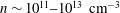 $n\sim 10^{11}{-}10^{13}~\text{cm}^{-3}$
and
$n\sim 10^{11}{-}10^{13}~\text{cm}^{-3}$
and
 $B\sim 10^{2}{-}10^{4}~\text{G}$
. Referring to table 1, we see these parameter ranges do not easily fit anywhere in the standard picture of the magnetosphere. Higher densities and much lower fields are needed. Perhaps the necessary magnetic loops or current sheets, if they do exist in the upper magnetosphere, have the right parameters; but no models yet predict such structures. Once again, new ideas are needed.
$B\sim 10^{2}{-}10^{4}~\text{G}$
. Referring to table 1, we see these parameter ranges do not easily fit anywhere in the standard picture of the magnetosphere. Higher densities and much lower fields are needed. Perhaps the necessary magnetic loops or current sheets, if they do exist in the upper magnetosphere, have the right parameters; but no models yet predict such structures. Once again, new ideas are needed.
8 Emission region of the High Frequency Interpulse
The spectral emission bands are not the only unusual property of the High Frequency Interpulse. Unlike Main Pulses and Low Frequency Interpulses, High Frequency Interpulses are partially dispersed within the magnetosphere before they leave the pulsar. In addition, their linear position angle shows no rotation across the entire mean profile component. Both properties give us additional clues on the origin of High Frequency Interpulses.

Figure 5. Excess dispersion measures, relative to Jodrell Bank monitoring, for 58 pulses captured within 80 minutes of each other during a typical observing day. (a) Shows
 ${\it\delta}(\text{DM})$
values for Main Pulses; (b) shows
${\it\delta}(\text{DM})$
values for Main Pulses; (b) shows
 ${\it\delta}(\text{DM})$
for High Frequency Interpulses. Observed at centre frequency 6500 MHz, with bandwidth 1 GHz; plotted against the rotation phase at which each pulse arrived (compare the mean profiles in figure 1). See Hankins et al. (Reference Hankins, Eilek and Jones2016) for details of method. The solid lines show the Jodrell Bank value (corresponding to
${\it\delta}(\text{DM})$
for High Frequency Interpulses. Observed at centre frequency 6500 MHz, with bandwidth 1 GHz; plotted against the rotation phase at which each pulse arrived (compare the mean profiles in figure 1). See Hankins et al. (Reference Hankins, Eilek and Jones2016) for details of method. The solid lines show the Jodrell Bank value (corresponding to
 ${\it\delta}(\text{DM})=0$
); the dotted lines are the mean
${\it\delta}(\text{DM})=0$
); the dotted lines are the mean
 ${\it\delta}(\text{DM})$
for each set of pulses. Dispersion of Main Pulses is approximately consistent with the Jodrell Bank value, but High Frequency Interpulses have significant intrinsic dispersion (
${\it\delta}(\text{DM})$
for each set of pulses. Dispersion of Main Pulses is approximately consistent with the Jodrell Bank value, but High Frequency Interpulses have significant intrinsic dispersion (
 ${\it\delta}(\text{DM})\neq 0$
), with large pulse-to-pulse scatter.
${\it\delta}(\text{DM})\neq 0$
), with large pulse-to-pulse scatter.
8.1 Intrinsic dispersion in the High Frequency Interpulse
To quantify magnetospheric dispersion, we use the dispersion measure (‘DM’), defined as follows. The signal propagation time from a cosmic source depends on the group velocity in the plasma through which it propagates:
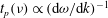 $t_{p}({\it\nu})\propto (\text{d}{\it\omega}/\text{d}k)^{-1}$
. For cold, weakly magnetized plasma (such as the interstellar medium), the dispersion relation is well known, and we have
$t_{p}({\it\nu})\propto (\text{d}{\it\omega}/\text{d}k)^{-1}$
. For cold, weakly magnetized plasma (such as the interstellar medium), the dispersion relation is well known, and we have
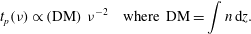 $$\begin{eqnarray}\displaystyle t_{p}({\it\nu})\propto (\text{DM})~{\it\nu}^{-2}\quad \text{where }\text{DM}=\int n\,\text{d}z. & & \displaystyle\end{eqnarray}$$
Thus, the difference in pulse arrival times at two frequencies measures the column density between the signal source and us. This quantity is conventionally expressed as the DM, with units of
 $\text{pc}~\text{cm}^{-3}$
 $(1~\text{pc}~\text{cm}^{-3}\simeq 3\times 10^{18}~\text{cm}^{-2})$
.
$(1~\text{pc}~\text{cm}^{-3}\simeq 3\times 10^{18}~\text{cm}^{-2})$
.
Nearly all of the dispersion for the Crab pulsar comes from the large plasma column between us and the pulsar – plasma in the Crab Nebula and the intervening interstellar medium. To focus on the small contribution from the pulsar itself, we express our results relative to the average DM which is tracked monthly by the Jodrell Bank Radio ObservatoryFootnote
8
. This excess DM for an individual pulse, relative to the Jodrell Bank value, we call
 ${\it\delta}(\text{DM})$
.
${\it\delta}(\text{DM})$
.
Figure 5 shows
 ${\it\delta}(\text{DM})$
values for Main Pulses and High Frequency Interpulses on a typical observing day. We find
${\it\delta}(\text{DM})$
values for Main Pulses and High Frequency Interpulses on a typical observing day. We find
 ${\it\delta}(\text{DM})$
for Main Pulses is approximately consistent with zero; the Jodrell Bank values describe the Main Pulse well. However,
${\it\delta}(\text{DM})$
for Main Pulses is approximately consistent with zero; the Jodrell Bank values describe the Main Pulse well. However,
 ${\it\delta}(\text{DM})$
for High Frequency Interpulses differs significantly from zero and fluctuates strongly from pulse to pulse. It can vary from nearly zero to
${\it\delta}(\text{DM})$
for High Frequency Interpulses differs significantly from zero and fluctuates strongly from pulse to pulse. It can vary from nearly zero to
 ${\sim}0.04~\text{pc}~\text{cm}^{-3}$
, on a time scale of a few minutes. We note that observations of Main Pulses and High Frequency Interpulses were interspersed with each other during a typical observing run. No intervening foreground ‘screen’ could change rapidly enough, and just in phase with the pulsar’s rotation, to exist only in front of the High Frequency Interpulse. It is therefore clear that the excess DM of the High Frequency Interpulse comes from the pulsar itself, not an intervening screen.
${\sim}0.04~\text{pc}~\text{cm}^{-3}$
, on a time scale of a few minutes. We note that observations of Main Pulses and High Frequency Interpulses were interspersed with each other during a typical observing run. No intervening foreground ‘screen’ could change rapidly enough, and just in phase with the pulsar’s rotation, to exist only in front of the High Frequency Interpulse. It is therefore clear that the excess DM of the High Frequency Interpulse comes from the pulsar itself, not an intervening screen.
We find no evidence that
 ${\it\delta}(\text{DM})$
depends on observing frequency between 5 and 30 GHz where we have captured High Frequency Interpulses. This suggests the magnetospheric dispersion law obeys
${\it\delta}(\text{DM})$
depends on observing frequency between 5 and 30 GHz where we have captured High Frequency Interpulses. This suggests the magnetospheric dispersion law obeys
 $t_{p}({\it\nu})\propto {\it\nu}^{-2}$
– although it need not be the cold plasma law assumed in (8.1). We note that a few
$t_{p}({\it\nu})\propto {\it\nu}^{-2}$
– although it need not be the cold plasma law assumed in (8.1). We note that a few
 ${\it\delta}(\text{DM})$
values in figure 5 are negative. We do not interpret this as inverted dispersion behaviour (
${\it\delta}(\text{DM})$
values in figure 5 are negative. We do not interpret this as inverted dispersion behaviour (
 $dt_{p}/d{\it\nu}>0$
) in the pulsar. Rather, it seems likely that the Jodrell Bank value, which is based on mean profiles, contains a small contribution, the mean excess dispersion,
$dt_{p}/d{\it\nu}>0$
) in the pulsar. Rather, it seems likely that the Jodrell Bank value, which is based on mean profiles, contains a small contribution, the mean excess dispersion,
 $\langle {\it\delta}(\text{DM})\rangle$
, from the pulsar itself.
$\langle {\it\delta}(\text{DM})\rangle$
, from the pulsar itself.
Interpreting our result in terms of plasma conditions in the emission region is difficult, because we do not know the true dispersion law in the region. Magnetospheric dispersion relations have been well studied only for low-altitude polar cap regions (e.g. Arons & Barnard Reference Arons and Barnard1986; Melrose & Gedalin Reference Melrose and Gedalin1999). While the effective DM has not been calculated for these laws, we suspect the more complex physical situation in such strongly magnetized regions would cause more complex
 $t_{p}({\it\nu})$
behaviour than the simple form in (8.1).
$t_{p}({\it\nu})$
behaviour than the simple form in (8.1).
As a possible example of dispersion in the upper magnetosphere, consider dispersion in a relativistic, weakly magnetized plasma. If
 $\langle {\it\gamma}\rangle$
measures the mean internal energy of the plasma, the DM over a path
$\langle {\it\gamma}\rangle$
measures the mean internal energy of the plasma, the DM over a path
 $L$
turns out to be
$L$
turns out to be
 $\simeq nL/\langle {\it\gamma}\rangle$
(following, e.g. Shcherbakov Reference Shcherbakov2008). Guessing
$\simeq nL/\langle {\it\gamma}\rangle$
(following, e.g. Shcherbakov Reference Shcherbakov2008). Guessing
 $L\sim 0.1R_{LC}$
for a high-altitude emission zone, we need
$L\sim 0.1R_{LC}$
for a high-altitude emission zone, we need
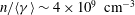 $n/\langle {\it\gamma}\rangle \sim 4\times 10^{9}~\text{cm}^{-3}$
to account for the typical
$n/\langle {\it\gamma}\rangle \sim 4\times 10^{9}~\text{cm}^{-3}$
to account for the typical
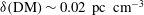 ${\it\delta}(\text{DM})\sim 0.02~\text{pc}~\text{cm}^{-3}$
we see in the High Frequency Interpulse. Comparing this result to the high-altitude GJ densities (table 1), we find a density enhancement
${\it\delta}(\text{DM})\sim 0.02~\text{pc}~\text{cm}^{-3}$
we see in the High Frequency Interpulse. Comparing this result to the high-altitude GJ densities (table 1), we find a density enhancement
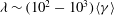 ${\it\lambda}\sim (10^{2}-10^{3})\langle {\it\gamma}\rangle$
would be needed. This is generally consistent with predictions of pair cascade models, as long as
${\it\lambda}\sim (10^{2}-10^{3})\langle {\it\gamma}\rangle$
would be needed. This is generally consistent with predictions of pair cascade models, as long as
 $\langle {\it\gamma}\rangle$
is not too large.
$\langle {\it\gamma}\rangle$
is not too large.
The more interesting clue, however, is the
 ${\it\delta}(\text{DM})$
variability. The plasma column around or above the emission site fluctuates by
${\it\delta}(\text{DM})$
variability. The plasma column around or above the emission site fluctuates by
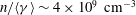 $n/\langle {\it\gamma}\rangle \sim 4\times 10^{9}~\text{cm}^{-3}$
, on time scales of no more than a few minutes. This shows the region creating the DM excess of the High Frequency Interpulse is not some high-density region that happens to sit above the emission zone. It must be an intrinsic part of the dynamic emission zone.
$n/\langle {\it\gamma}\rangle \sim 4\times 10^{9}~\text{cm}^{-3}$
, on time scales of no more than a few minutes. This shows the region creating the DM excess of the High Frequency Interpulse is not some high-density region that happens to sit above the emission zone. It must be an intrinsic part of the dynamic emission zone.

Figure 6. Polarization of two High Frequency Interpulses, captured between 17.75 and 22.75 GHz, within two minutes of each other on one observing day. Dedispersed with DM
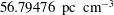 $56.79476~\text{pc}~\text{cm}^{-3}$
and displayed with 51.2 ns time resolution. The pulse in (a,c) arrived close to the leading edge of the High Frequency Interpulse component in the mean profile (figure 1); the pulse shown in (b,d) arrived close to the trailing edge. For each pulse, (a,b) shows the total flux (I; solid line) and linearly polarized flux (L; green filled area). (c,d) shows the position angle of the linear polarization (
$56.79476~\text{pc}~\text{cm}^{-3}$
and displayed with 51.2 ns time resolution. The pulse in (a,c) arrived close to the leading edge of the High Frequency Interpulse component in the mean profile (figure 1); the pulse shown in (b,d) arrived close to the trailing edge. For each pulse, (a,b) shows the total flux (I; solid line) and linearly polarized flux (L; green filled area). (c,d) shows the position angle of the linear polarization (
 ${\it\phi}$
). Polarization is shown only for points above three times the off-pulse noise (indicated by the two orange lines in (a,b)).
${\it\phi}$
). Polarization is shown only for points above three times the off-pulse noise (indicated by the two orange lines in (a,b)).
8.2 Linear polarization in the High Frequency Interpulse
High Frequency Interpulses are linearly polarized. Figure 6 shows two typical pulses, both of which are strongly polarized with nearly constant position angles. The polarization provides two key diagnostics of the emission region for this component.
Such strong polarization – 90 % is typical – constrains the extent of the emission region. We argued in § 2.3 that the phase coincidence of the High Frequency Interpulse and the high-energy pulse P2 suggests the two features originate in similar parts of the magnetosphere. However, if the High Frequency Interpulse comes from a wide range of altitudes – say throughout a slot gap or an outer gap – it would be depolarized by caustic effects (Dyks et al. Reference Dyks, Harding and Rudak2004). The strong polarization of the High Frequency Interpulse tells us caustic depolarization is not important for this component. Therefore, its emission zone must occupy only a small fraction of the extended caustic region that is probably the source of pulsed high-energy emission.
Figure 6 also shows that the polarized position angle remains constant throughout a single pulse. This angle is independent of the rotation phase at which the pulse appears. For example, the two pulses in figure 6 arrived at rotation phases separated by
 $6.5^{\circ }$
(which can be compared to the
$6.5^{\circ }$
(which can be compared to the
 $9.0^{\circ }$
width of the mean profile component; Hankins et al.
Reference Hankins, Jones and Eilek2015), yet both pulses show the same, steady polarization angle.
$9.0^{\circ }$
width of the mean profile component; Hankins et al.
Reference Hankins, Jones and Eilek2015), yet both pulses show the same, steady polarization angle.
The position angle of pulsar radio emission reveals the direction of the magnetic field in the emission zone. Radio emission is polarized either parallel or perpendicular to the local field, depending on the emission model. The polarization angle observed at earth therefore depends on the direction of the field as projected on the sky plane. A change of angle through a pulse is interpreted as a change of magnetic field direction. The classic example is radiation from the low-altitude polar gap, which is a region with diverging field lines. As the star rotates past the line of sight, creating the radio pulse, the projected field direction rotates across the pulse (e.g. Radhakrishnan & Cooke Reference Radhakrishnan and Cooke1969).
The lack of such position-angle rotation in the High Frequency Interpulse tells us the direction of the magnetic field is constant throughout its emission region. The field does not diverge within the region, as it does in the polar gap. Its direction does not change with time, as might be expected in a turbulent region dominated by plasma inertia. The emission region for the High Frequency Interpulse must be inhomogeneous – in order to account for the variable dispersion – but must also contain an ordered magnetic field. Perhaps we are seeing a region filled with field-aligned density fluctuations.
9 Summary and lessons learned
In this paper we have reviewed our high-time-resolution observations of the Crab pulsar and compared them to various models for pulsar radio emission physics. We offer hearty congratulations to the reader who has made it this far. To summarize, our key results are as follows.
-
(i) The bright radio pulses come from high altitudes, not from the polar caps. Their emission regions are probably co-spatial with the gaps or current sheets responsible for high-energy emission. We use our data to probe physical conditions in the outer reaches of the magnetosphere.
-
(ii) Variability of the radio signal on microsecond time scales, or longer, is generally consistent with the picture of cyclic pair cascades in an unshielded gap. The details, however, remain unclear; we suggest our radio data motivate new study of cascades in high-altitude emission regions.
-
(iii) Three emission models – strong plasma turbulence, free-electron masers, and cyclotron instability emission – compare fairly well to the nanoshots which characterize the Main Pulse and the Low Frequency Interpulse. However, none of them can explain all of the observations; further work is needed.
-
(iv) The spectral emission bands which characterize the High Frequency Interpulse confound every radio emission model yet proposed. The model which comes closest is double-resonant emission, but it requires extreme conditions which push the envelope of current magnetosphere models.
-
(v) The variable dispersion and strong polarization of the High Frequency Interpulse show the emission zone for that component is a localized, dynamic region that is probably threaded by a uniform magnetic field.
Our analysis makes it clear that we do not yet have all the answers about the pulsar’s magnetosphere and how it makes coherent radio emission. We have, however, learned some useful lessons which should help us going forward.
The Crab pulsar has at least one radio emission zone that is not predicted by current models. Strong radio pulses from the Crab pulsar come from localized zones within extended high-energy emission regions – probably gaps or separatrices associated with each magnetic pole. We infer this from several facts. The Main Pulse and the Low Frequency Interpulse appear at the same rotation phases as the two strong components of the high-energy mean profile, and the viewing angle of the star does not allow a low-altitude polar cap origin for the latter. Furthermore, these two components have the same radio characteristics. This suggests they come from the same emission physics, which is consistent with their origin in two similar regions connected to the two magnetic poles.
The story is much less clear, however, for a third radio component. The High Frequency Interpulse has very different characteristics from the other two. This suggests it comes from a region in which different emission physics is operating, but we do not know where that is. Because the High Frequency and Low Frequency Interpulses appear at similar rotation phases, we might think they come from different parts of one polar caustic. However, the most likely models suggest the High Frequency Interpulse arises in a dense, turbulent region with uniform magnetic field direction. It is not clear where such a region exists within our current picture of the high-altitude magnetosphere.
High-altitude emission zones are unsteady places. Their dynamical state is reflected in the radio emission. Radio emission from the Crab pulsar is not steady. It comes in short-lived bursts which can occur anywhere within the probability envelope defined by the mean profile. We conclude from this that the mechanism which drives the coherent radio emission exists only sporadically throughout the emission zone. Whatever drives the driver must also be sporadic. The energy source builds up, is depleted to radio emission and is soon regenerated to repeat the cycle.
If the driver is a relativistic particle beam – as is likely for the Main Pulse and Low Frequency Interpulse – the duty cycle reflects oscillatory behaviour of parallel electric fields which drive the beams. This picture is generally consistent with the behaviour expected for unsteady pair cascades in gap regions. If the Main Pulse and Low Frequency Interpulse come from high-altitude caustic regions associated with the star’s two magnetic poles, an unsteady ‘sparking’ cycle must occur there, just as has been predicted for the low-altitude polar cap.
The driver is less certain for the High Frequency Interpulse, because its radio emission mechanism is less clear. Perhaps unsteady reconnection is taking place in the mysterious region which gives rise to this component.
The radio emission regions are either denser, or more tenuous, than predicted by standard pair cascade models, but we do not know which. Radio bursts in Main Pulses and Low Frequency Interpulses are clumps of nanoshots: short-lived narrowband polarized flashes of radio emission. No models yet proposed can fully explain the nanoshots, but some come close. One class of models involves strong plasma turbulence, either directly (via soliton collapse) or indirectly (via the bunched response of the driving beam). These models require fairly low densities within the emission zones – comparable to, or somewhat above, the GJ density. An alternative model invokes emission from a cyclotron instability. This model requires substantially higher densities in the emission zones, significantly above the GJ density for the region and also well above densities predicted by current pair cascade models. None of these models are the final word on the nanoshots, but all of them appear to disagree with predictions of the pair cascade models.
Two other arguments also suggest high densities. While the emission physics behind the High Frequency Interpulse is not well understood, the promising double-resonant model of the spectral bands requires high densities in the relevant emission zone. In addition, some models of the Crab’s pulsar wind nebula require high densities in the wind leaving the pulsar. Neither of these models is likely to be the final word on the High Frequency Interpulse or the nebular wind, but both suggest densities higher than pair cascade models can produce. We conclude that the pair cascade – the only mechanism yet proposed to increase magnetospheric density over the fiducial GJ value – is not yet understood.
Radio emission can be a powerful probe of magnetospheric conditions, but the models need more work. We have discussed the radio emission models we find the most promising at present, and the limitations of each one. Models based on plasma turbulent emission have been extended to nonlinear regimes, and thus can address short-lived nanoshots. However, they are restricted to electrostatic turbulence in strongly magnetized regions, so they cannot account for circular polarization in the nanoshots. Models based on cyclotron emission have been constructed to admit circular polarization. However, they have not been developed past the linear regime, so they cannot address the behaviour of the nanoshots. Models based on solar zebra bands are a promising approach to the spectral emission bands, but they require unusual physical situations which are not part of our standard picture of the magnetosphere.
Our opinion is that these models – which we have highlighted – can benefit by continued development, and help us truly understand conditions in the high-altitude radio emission zones. These are not the only options, however. Many other models, including those listed in appendix A, have promise but have not been developed to the point where they can be compared to data in any quantitative way. Perhaps one of them will turn out, in the end, to be a better answer for radio emission from the Crab pulsar.
Acknowledgements
We are grateful to G. Benford, M. Lyutikov and D. Melrose for entertaining discussions and thoughtful reviews that have helped our understanding and appreciation of pulsar emission physics. We particularly thank G. Jones and many of our students, including D. Moffett, J. Kern, J. Crossley, T. Delaney, E. Plum, J. Dickerson, and J. Sheckard for their critical help at the telescopes during our observing sessions. The Arecibo Observatory is operated by SRI International under a cooperative agreement with the National Science Foundation, and in alliance with Ana G. Méndez-Universidad Metropolitana and the Universities Space Research Association. The Very Large Array and the Green Bank Telescope are run by the National Radio Astronomy Observatory, a facility of the National Science Foundation, operated under cooperative agreement by Associated Universities, Inc.
Appendix A. Models proposed for pulsar radio emission
A wide range of models have been proposed over the years to explain the mechanism by which pulsars make coherent radio emission. The models vary in both the plasma-scale processes responsible for the radiation and the magnetosphere conditions under which they can operate.
We do not attempt to give a full review of all possible radio emission models. The reader who has the strength can refer to the excellent reviews by Melrose (such as Melrose Reference Melrose1995) for a more complete discussion. Instead, we present overviews of several models which are commonly proposed and/or of particular interest for the Crab pulsar.
A.1 Strong plasma turbulence
This mechanism is known to operate in solar radio bursts, but must be revisited for the high magnetic fields and relativistic pair plasmas relevant to pulsars. An instability – most likely two-stream, driven by an energetic particle beam – drives Langmuir turbulence. That turbulence cannot escape the plasma directly; the Langmuir waves must undergo some nonlinear process which converts part or all of their energy into escaping radiation.
One possibility for this mode conversion involves modulational instabilities in strong Langmuir turbulence that drive the growth (‘collapse’) of localized knots of strong electric field, generally called solitons. Nonlinear wave–wave coupling within the solitons generates bursts of electromagnetic radiation – ‘nanoshots’ – which can escape the plasma (e.g. Robinson Reference Robinson1997). Weatherall (Reference Weatherall1997, Reference Weatherall1998) has studied this process in the pulsar context.
The duration and spectrum of the nanoshots provide key comparisons to the data. In Weatherall’s simulations, the rate of collapse of the electrostatic wave packet and subsequent conversion to electromagnetic modes is of the order of
 ${\sim}{\it\Lambda}{\it\nu}_{p}$
, where
${\sim}{\it\Lambda}{\it\nu}_{p}$
, where
 ${\it\nu}_{p}$
is the plasma frequency, and
${\it\nu}_{p}$
is the plasma frequency, and
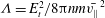 ${\it\Lambda}=E_{t}^{2}/8{\rm\pi}nm\bar{v_{\Vert }}^{2}$
measures the strength of the turbulence (
${\it\Lambda}=E_{t}^{2}/8{\rm\pi}nm\bar{v_{\Vert }}^{2}$
measures the strength of the turbulence (
 $E_{t}$
is the turbulent wave electric field and
$E_{t}$
is the turbulent wave electric field and
 $\bar{v_{\Vert }}$
is the velocity spread of the pair plasma). The time scale for soliton collapse, and the duration of the nanoshot produced by each collapse, is therefore
$\bar{v_{\Vert }}$
is the velocity spread of the pair plasma). The time scale for soliton collapse, and the duration of the nanoshot produced by each collapse, is therefore
 ${\it\delta}t\sim 1/{\it\Lambda}{\it\nu}_{p}$
. The spectrum of the nanoshot will be relatively narrowband,
${\it\delta}t\sim 1/{\it\Lambda}{\it\nu}_{p}$
. The spectrum of the nanoshot will be relatively narrowband,
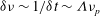 ${\it\delta}{\it\nu}\sim 1/{\it\delta}t\sim {\it\Lambda}{\it\nu}_{p}$
. Weatherall found that strong, localized solitons appear for
${\it\delta}{\it\nu}\sim 1/{\it\delta}t\sim {\it\Lambda}{\it\nu}_{p}$
. Weatherall found that strong, localized solitons appear for
 ${\it\Lambda}\gtrsim 0.1$
.
${\it\Lambda}\gtrsim 0.1$
.
Weatherall’s calculation assumes the radiative loss time scale is no longer than dynamic time scale for soliton collapse. This holds for packet sizes smaller than
 ${\sim}c/{\it\Lambda}{\it\nu}_{p}$
, which is consistent with other estimates of soliton size (e.g. Weatherall & Benford Reference Weatherall and Benford1991).
${\sim}c/{\it\Lambda}{\it\nu}_{p}$
, which is consistent with other estimates of soliton size (e.g. Weatherall & Benford Reference Weatherall and Benford1991).
Polarization of the nanoshot is another key test. The collapsing soliton generates electromagnetic waves with polarization set by local plasma conditions. Weatherall (Reference Weatherall1998) worked in the context of a strongly magnetized plasma. In this limit, emergent radiation around the plasma frequency – such as the nanoshots – is linearly polarized along the magnetic field (cf. the O mode of Arons & Barnard Reference Arons and Barnard1986).
Because strong Langmuir turbulence is an incoherent superposition of localized solitons (e.g. Robinson Reference Robinson1997), the radiation ‘shot’ produced by each soliton is independent of those from its neighbours. This agrees nicely with the amplitude-modulated noise model suggested by high-time-resolution observations of pulsar radio emission (Rickett Reference Rickett1975, also § 5.3). We compare this model to the Crab pulsar in § 6.1.
A.2 Free-electron maser emission
In this model, a relativistic beam encounters an electric field that varies in space and time. Charges interacting with the field bunch together in a resonant interaction, and emit intense, coherent bursts of radiation. This process has been extensively studied in the lab, where particle beams pass through externally applied electromagnetic fields (‘wigglers’) and radiate in a narrow cone beamed along the initial beam direction.
This interesting idea has not been taken very far in pulsar applications. Fung & Kuijpers (Reference Fung and Kuijpers2004) proposed a model in which a high-
 ${\it\gamma}$
beam propagates through a strong, transverse EM wiggler in a nearly unmagnetized background plasma. Their simulations found the expected collective particle bunching, resulting in short-lived narrowband bursts of radiation, on a time scale governed by the frequency of the imposed EM wiggler. However, neither an externally applied transverse wiggler, nor a nearly unmagnetized plasma, seem easy to maintain in a pulsar magnetosphere.
${\it\gamma}$
beam propagates through a strong, transverse EM wiggler in a nearly unmagnetized background plasma. Their simulations found the expected collective particle bunching, resulting in short-lived narrowband bursts of radiation, on a time scale governed by the frequency of the imposed EM wiggler. However, neither an externally applied transverse wiggler, nor a nearly unmagnetized plasma, seem easy to maintain in a pulsar magnetosphere.
A more likely possibility is that the particle beam generates its own parallel wiggler. Baker et al. (Reference Baker, Borovsky, Benford and Eilek1988), also Weatherall & Benford (Reference Weatherall and Benford1991), suggested that when beam-driven Langmuir turbulence becomes strong, both it and the driving beam will become spatially inhomogeneous. In that situation, the collective motion of charge bunches interacting with electrostatic fluctuations in the turbulence results in coherent, forward-beamed radiation (e.g. Kato, Benford & Tzach Reference Kato, Benford and Tzach1983; Schopper et al.
Reference Schopper, Ruhl, Kunzl and Lesch2003). For weak Langmuir turbulence, these models predict linearly polarized radiation at
 ${\sim}{\it\gamma}^{2}{\it\nu}_{p}$
, where
${\sim}{\it\gamma}^{2}{\it\nu}_{p}$
, where
 ${\it\nu}_{p}$
is the plasma frequency of the background plasma. If turbulence is strong enough to collapse to solitons with scale
${\it\nu}_{p}$
is the plasma frequency of the background plasma. If turbulence is strong enough to collapse to solitons with scale
 $D<c/{\it\omega}_{p}$
, the Compton-boosted beam radiation comes out at even higher frequencies
$D<c/{\it\omega}_{p}$
, the Compton-boosted beam radiation comes out at even higher frequencies
 ${\sim}{\it\gamma}_{b}^{2}c/D$
(Weatherall & Benford Reference Weatherall and Benford1991). In either case, the radiation frequency is significantly boosted relative to the plasma frequency of the background plasma. We consider this for the Crab pulsar in § 6.2.
${\sim}{\it\gamma}_{b}^{2}c/D$
(Weatherall & Benford Reference Weatherall and Benford1991). In either case, the radiation frequency is significantly boosted relative to the plasma frequency of the background plasma. We consider this for the Crab pulsar in § 6.2.
A.3 Cycloton instability emission
In this model, a relativistic particle beam drives a cyclotron instability through the cyclotron resonance,
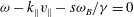 ${\it\omega}-k_{\Vert }v_{\Vert }-s{\it\omega}_{B}/{\it\gamma}=0$
. Initially the
${\it\omega}-k_{\Vert }v_{\Vert }-s{\it\omega}_{B}/{\it\gamma}=0$
. Initially the
 $s=1$
resonance was invoked as a source of Alfvén waves that could scatter particles to higher pitch angles as they passed into the wind, thus enabling synchrotron radiation (Machabeli & Usov Reference Machabeli and Usov1979) from the wind nebula.
$s=1$
resonance was invoked as a source of Alfvén waves that could scatter particles to higher pitch angles as they passed into the wind, thus enabling synchrotron radiation (Machabeli & Usov Reference Machabeli and Usov1979) from the wind nebula.
Later authors, including Kazbegi et al. (Reference Kazbegi, Machabeli and Melikidze1991) and Lyutikov et al. (Reference Lyutikov, Machabeli and Blandford1999), suggested the anomalous cyclotron instability (
 $s<0$
) could be a direct radiation source, generating transverse waves which escape the plasma without needing mode conversion. This interaction causes a beam particle to increase its perpendicular momentum, at the same time that it emits a photon; the energy of course comes from the parallel momentum. If wave modes in the background plasma are circularly polarized – as is assumed in their formulation – the emitted radiation is also circularly polarized.
$s<0$
) could be a direct radiation source, generating transverse waves which escape the plasma without needing mode conversion. This interaction causes a beam particle to increase its perpendicular momentum, at the same time that it emits a photon; the energy of course comes from the parallel momentum. If wave modes in the background plasma are circularly polarized – as is assumed in their formulation – the emitted radiation is also circularly polarized.
In practice, this model is challenged in application to real pulsars, because of the weak magnetic fields and high plasma densities needed in order to put the emitted radiation in the radio band. It is also challenged by the lack of a clear path to produce short-lived nanoshots. We consider this model for the Crab pulsar in § 6.3.
A.4 Linear acceleration emission
In this model, a beam of relativistic charges moving along a magnetic field passes through and responds to an oscillating, parallel electric field. The particles radiate due to the acceleration caused by
 $E_{\Vert }$
. Melrose (Reference Melrose1978) treated this process in the linear limit (assuming
$E_{\Vert }$
. Melrose (Reference Melrose1978) treated this process in the linear limit (assuming
 ${\it\gamma}$
stays nearly constant), and showed that the radiation comes out around
${\it\gamma}$
stays nearly constant), and showed that the radiation comes out around
 ${\it\gamma}^{2}{\it\omega}_{o}$
, where
${\it\gamma}^{2}{\it\omega}_{o}$
, where
 ${\it\omega}_{o}$
is the oscillation frequency of the E field. The radiation is linearly polarized parallel to the projected B field. To reach high brightness temperatures while retaining the single-particle linear analysis, Melrose suggested negative absorption (maser amplification), but found the optical depth is much less than unity for typical pulsar conditions.
${\it\omega}_{o}$
is the oscillation frequency of the E field. The radiation is linearly polarized parallel to the projected B field. To reach high brightness temperatures while retaining the single-particle linear analysis, Melrose suggested negative absorption (maser amplification), but found the optical depth is much less than unity for typical pulsar conditions.
The origin of the oscillating E field is unclear. Melrose (Reference Melrose1978) suggested oscillation at
 ${\sim}{\it\omega}_{p}$
, a case which is very similar to free-electron maser models when the wigglers are self-generated Langmuir waves. Unsteady pair creation in an unshielded gap has also been suggested as the source of oscillating E fields (e.g. Levinson et al.
Reference Levinson, Melrose, Judge and Luo2005; Timokhin & Arons Reference Timokhin and Arons2013). These models are still being developed, and the time signature of the unshielded E field is not yet clear. In addition, recent work has explored electric fields strong enough to change the particle’s Lorentz factor significantly in one oscillation. This limit seems more relevant to high-energy emission, and different treatments are still being explored in the literature (Melrose, Rafat & Luo Reference Melrose, Rafat and Luo2009; Reville & Kirk Reference Reville and Kirk2010). We find this mechanism interesting, but further work is needed before it can be usefully tested against pulsar data.
${\sim}{\it\omega}_{p}$
, a case which is very similar to free-electron maser models when the wigglers are self-generated Langmuir waves. Unsteady pair creation in an unshielded gap has also been suggested as the source of oscillating E fields (e.g. Levinson et al.
Reference Levinson, Melrose, Judge and Luo2005; Timokhin & Arons Reference Timokhin and Arons2013). These models are still being developed, and the time signature of the unshielded E field is not yet clear. In addition, recent work has explored electric fields strong enough to change the particle’s Lorentz factor significantly in one oscillation. This limit seems more relevant to high-energy emission, and different treatments are still being explored in the literature (Melrose, Rafat & Luo Reference Melrose, Rafat and Luo2009; Reville & Kirk Reference Reville and Kirk2010). We find this mechanism interesting, but further work is needed before it can be usefully tested against pulsar data.
A.5 Maser amplification of radio beams
Lyubarskii & Petrova (Reference Lyubarskii and Petrova1996) considered stimulated Compton scattering of pulsar radio emission by the magnetospheric pair plasma in the presence of background radiation. They were interested in scattering out of the radio beam, to explain low-frequency spectral turnovers seen in many pulsars. However in later papers, (e.g. Petrova Reference Petrova2008, Reference Petrova2009) suggested that stimulated scattering of radio emission out of the primary beam can be the origin of secondary components in a pulsar’s mean profile (e.g. the interpulse found in a few radio pulsars, or the several components of the Crab’s mean profile). Unfortunately, the scattering opacity is hard to predict. It depends not just on magnetospheric parameters, but also varies with scattering regimes, so that the nature of the scattered radiation is extremely sensitive to assumed details of the scattering. While these models have some nice physics, the difficulty of quantifying the scattering opacity seems to preclude any robust test of them against the data.
Weatherall (Reference Weatherall2001) also considered stimulated Compton scattering of a pulsar radio beam, but by strong turbulence in the magnetospheric plasma which the beam traverses. He mostly studied scattering in a non-magnetized plasma, but did include a simple model restricting charge motion to one dimension (appropriate for a high magnetic field). He finds that interesting amplification is possible if the plasma turbulence is extremely strong (e.g. turbulent energy density of the order of
 $10^{12}$
times the plasma temperature). However, he presents no discussion of how such strong turbulence can be maintained, nor does he consider radiation emitted by the turbulence itself (as in § A.1 above).
$10^{12}$
times the plasma temperature). However, he presents no discussion of how such strong turbulence can be maintained, nor does he consider radiation emitted by the turbulence itself (as in § A.1 above).
In addition, both of these models assume the existence of an initial radio beam that can be amplified by stimulated scattering. The origin of the beam is not discussed. In that sense, neither of these models addresses the primary radio emission mechanism. Given the many uncertainties, neither model can easily be compared to radio data. We do not pursue these any further.
A.6 Coherent charge bunches
Curvature emission by coherent bunches was one of the first models proposed for pulsar radio emission (e.g. Ruderman & Sutherland Reference Ruderman and Sutherland1975; Buschauer & Benford Reference Buschauer and Benford1976). The general idea is that some instability groups
 $N\gg 1$
charges into a coherently moving bunch that acts as a single large charge,
$N\gg 1$
charges into a coherently moving bunch that acts as a single large charge,
 $Q=Ne$
; this bunch then radiates curvature emission in the radio band. Although this model initially seemed attractive, subsequent analysis (e.g. Melrose Reference Melrose1978, Reference Melrose1995, and references therein) identified several serious problems, including but not limited to the lack of an effective mechanism for forming the bunches, and the inability of the putative charge bunch to hold together long enough to radiate.
$Q=Ne$
; this bunch then radiates curvature emission in the radio band. Although this model initially seemed attractive, subsequent analysis (e.g. Melrose Reference Melrose1978, Reference Melrose1995, and references therein) identified several serious problems, including but not limited to the lack of an effective mechanism for forming the bunches, and the inability of the putative charge bunch to hold together long enough to radiate.
This model has recently been revived by Melikidze, Gil & Pataraya (Reference Melikidze, Gil and Pataraya2000; also Gil, Lyubarsky & Melikidze Reference Gil, Lyubarsky and Melikidze2004). They follow Karpman et al. (Reference Karpman, Norman, Ter Harr and Tsytovich1975), who argued that Langmuir solitons will be charge separated if the two charge species have different masses. Melikidze et al. (Reference Melikidze, Gil and Pataraya2000) proposed that solitons in a pair plasma will also be charge separated if the electrons and positrons have different relativistic streaming speeds. These authors then assumed that the solitons are sufficiently long lived for the separated ‘charges’ within each soliton to produce curvature emission. They further assumed that the plasma and soliton parameters are just what is needed to put the radiation in the radio band, and they ignored any other radiation caused by plasma dynamics within the soliton. Given the large number of assumptions required by this model, and the lack of any demonstration of the solitons’ dynamic evolution, we do not consider this model any further.
A.7 Curvature maser emission
While simple curvature emission cannot support maser action (Blandford Reference Blandford1975), signal amplification is possible if particle curvature drift and/or field line distortion is taken into account (e.g. Luo & Melrose Reference Luo and Melrose1992, Reference Luo and Melrose1995; Lyutikov et al. Reference Lyutikov, Machabeli and Blandford1999). However, the model details are very sensitive to the local field line curvature, which is poorly known in the outer magnetosphere. The situation is also complicated by the fact that the energetic particle beam necessary for either type of curvature maser also drives streaming instabilities that can lead to relativistic plasma emission (see Melrose Reference Melrose1995). Furthermore, there is still disagreement in the literature about the efficacy of this mechanism (e.g. Kaganovich & Lyubarsky Reference Kaganovich and Lyubarsky2010). For all of these reasons, we do, not pursue this mechanism here.
Appendix B. Double plasma resonance model for pulsar emission
The spectral emission bands in the High Frequency Interpulse have not been seen in any other pulsar. A variety of new models, specific to the emission bands, have been suggested since their discovery, but none have successfully explained all the data. We review several such models in Hankins et al. (Reference Hankins, Eilek and Jones2016); here we only discuss one, the Double Plasma Resonance which may explain the ‘zebra’ emission bands seen in Type IV solar flares (e.g. Kuijpers Reference Kuijpers1975; Zhelezniakov & Zlotnik Reference Zhelezniakov and Zlotnik1975; Winglee & Dulk Reference Winglee and Dulk1986).
This is another two-stage process. A maser instability generates upper hybrid waves at the cyclotron resonance, and those waves must be converted to transverse modes in order to escape the system. The instability growth is especially rapid at a set of discrete frequencies,
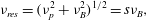 $$\begin{eqnarray}\displaystyle {\it\nu}_{res}=({\it\nu}_{p}^{2}+{\it\nu}_{B}^{2})^{1/2}=s{\it\nu}_{B}, & & \displaystyle\end{eqnarray}$$
where
 $s$
is the harmonic number,
$s$
is the harmonic number,
 ${\it\nu}_{p}$
is the plasma frequency,
${\it\nu}_{p}$
is the plasma frequency,
 ${\it\nu}_{B}$
is the electron cyclotron frequency and the growth is fastest for waves propagating across the local magnetic field.
${\it\nu}_{B}$
is the electron cyclotron frequency and the growth is fastest for waves propagating across the local magnetic field.
If the plasma is non-uniform, with the magnetic field and plasma density varying on different scales, the resonance for each harmonic
 $s$
will be satisfied at a different spatial location, and multiple spectral bands will be seen. This is a stringent constraint. In order to produce a particular value of the band spacing,
$s$
will be satisfied at a different spatial location, and multiple spectral bands will be seen. This is a stringent constraint. In order to produce a particular value of the band spacing,
 ${\rm\Delta}{\it\nu}/{\it\nu}$
, the local structure of the plasma density and magnetic field must have just the right behaviour. From (B 1), in the limit
${\rm\Delta}{\it\nu}/{\it\nu}$
, the local structure of the plasma density and magnetic field must have just the right behaviour. From (B 1), in the limit
 ${\it\nu}_{B}\ll {\it\nu}_{p}$
, the spacing between adjacent bands is usually written
${\it\nu}_{B}\ll {\it\nu}_{p}$
, the spacing between adjacent bands is usually written
 $$\begin{eqnarray}\displaystyle \frac{{\rm\Delta}{\it\nu}}{{\it\nu}}\simeq \frac{L_{B}}{sL_{B}-(s+1)L_{n}}, & & \displaystyle\end{eqnarray}$$
where
 $L_{B}$
and
$L_{B}$
and
 $L_{n}$
are the gradient scales of the magnetic field and density:
$L_{n}$
are the gradient scales of the magnetic field and density:
 $L_{B}=B/|\boldsymbol{{\rm\nabla}}B|$
and
$L_{B}=B/|\boldsymbol{{\rm\nabla}}B|$
and
 $L_{n}=2n/|\boldsymbol{{\rm\nabla}}n|$
. For general field and density distributions,
$L_{n}=2n/|\boldsymbol{{\rm\nabla}}n|$
. For general field and density distributions,
 $L_{B}$
and
$L_{B}$
and
 $L_{n}$
are functions of position, and (B 2) becomes an implicit condition for the location at which (B 1) is satisfied for a given harmonic
$L_{n}$
are functions of position, and (B 2) becomes an implicit condition for the location at which (B 1) is satisfied for a given harmonic
 $s$
.
$s$
.
In addition to the geometrical restriction, this theory has other important requirements on the plasma. The magnetic field must be weak,
 ${\it\nu}_{B}\ll {\it\nu}_{p}$
, and much lower than is predicted anywhere in the standard magnetosphere if
${\it\nu}_{B}\ll {\it\nu}_{p}$
, and much lower than is predicted anywhere in the standard magnetosphere if
 ${\it\nu}_{res}$
is to lie in the radio band. The theory has only been developed for non-relativistic, electron–ion plasmas. Zheleznyakov et al. (Reference Zheleznyakov, Zaitsev and Zlotnik2012) suggested the instability may also develop in pair plasmas, but we have not found that work in the literature. There must be an excess of energetic particles moving across the magnetic field – a situation which is common in solar coronal loops, but not expected in the standard magnetosphere.
${\it\nu}_{res}$
is to lie in the radio band. The theory has only been developed for non-relativistic, electron–ion plasmas. Zheleznyakov et al. (Reference Zheleznyakov, Zaitsev and Zlotnik2012) suggested the instability may also develop in pair plasmas, but we have not found that work in the literature. There must be an excess of energetic particles moving across the magnetic field – a situation which is common in solar coronal loops, but not expected in the standard magnetosphere.
Despite the challenges, we find this model attractive, because it offers a clear physical cause of discrete spectral bands such as those we see in the High Frequency Interpulse of the Crab pulsar. We discuss its relevance for the Crab pulsar in § 7.3.