1 Introduction
This paper discusses results from optimizations to produce quasi-helically symmetric (QHS) equilibria that simultaneously demonstrate multiple desirable properties for advanced stellarators. These properties include excellent neoclassical and energetic particle confinement, a reduction in turbulent transport and a functional non-resonant divertor (Bader et al. Reference Bader, Boozer, Hegna, Lazerson and Schmitt2017; Boozer & Punjabi Reference Boozer and Punjabi2018). The baseline targets for the configuration also avoided low-order rational surfaces, and included a vacuum magnetic well to avoid interchange instabilities. In this paper, we present a configuration that includes both the desired confinement and global macroscopic properties.
Optimization studies of stellarators have a long and rich history (Grieger et al. Reference Grieger, Lotz, Merkel, Nührenberg, Sapper, Strumberger, Wobig, Burhenn, Erckmann and Gasparino1992). The two constructed optimized stellarator experiments to date are the QHS Helically Symmetric eXperiment (HSX) (Anderson et al. Reference Anderson, Simon, Almagri, Anderson, Matthews, Talmadge and Shohet1995) and the quasi-omnigenous Wendelstein 7-X (W7-X) (Beidler et al. Reference Beidler, Grieger, Herrnegger, Harmeyer, Kisslinger, Lotz, Maassberg, Merkel, Nührenberg and Rau1990). Examples of quasi-axisymmetric stellarator concepts are the National Compact Stellarator eXperiment (NCSX) (Zarnstorff et al. Reference Zarnstorff, Berry, Brooks, Fredrickson, Fu, Hirshman, Hudson, Ku, Lazarus and Mikkelsen2001) and the Chinese First Quasi-axisymmetric Stellarator (Shimizu et al. Reference Shimizu, Liu, Isobe, Okamura, Nishimura, Suzuki, Xu, Zhang, Liu and Huang2018). Optimized stellarator configurations have also been the focus of reactor concepts. These include the ARIES-CS project (Ku et al. Reference Ku, Garabedian, Lyon, Turnbull, Grossman, Mau and Zarnstorff2008) adapted from the NCSX design, the HELIAS reactor concept (Beidler et al. Reference Beidler, Harmeyer, Herrnegger, Igitkhanov, Kendl, Kisslinger, Kolesnichenko, Lutsenko, Nührenberg and Sidorenko2001) adapted from W7-X and the Stellarator Pilot Plant Study (Miller et al Reference Miller1996) a quasi-helical configuration adapted from HSX.
Improvements in optimization tools have led to new configuration designs. These advances come in several forms including the identification of new quasi-axisymmetric configurations (Henneberg et al. Reference Henneberg, Drevlak, Nührenberg, Beidler, Turkin, Loizu and Helander2019b). Advances in theoretical understanding have produced mechanisms for optimization in the areas of turbulent transport (Mynick, Pomphrey & Xanthopoulos Reference Mynick, Pomphrey and Xanthopoulos2010; Xanthopoulos et al. Reference Xanthopoulos, Mynick, Helander, Turkin, Plunk, Jenko, Görler, Told, Bird and Proll2014; Hegna, Terry & Faber Reference Hegna, Terry and Faber2018), energetic particle transport (Bader et al. Reference Bader, Drevlak, Anderson, Faber, Hegna, Likin, Schmitt and Talmadge2019; Henneberg, Drevlak & Helander Reference Henneberg, Drevlak and Helander2019a) and non-resonant divertors (Bader et al. Reference Bader, Hegna, Cianciosa and Hartwell2018). Also, construction of optimized equilibria from first principles has been demonstrated for quasi-symmetric stellarators (Landreman & Sengupta Reference Landreman and Sengupta2018; Landreman, Sengupta & Plunk Reference Landreman, Sengupta and Plunk2019) and quasi-omnigenous stellarators (Plunk, Landreman & Helander Reference Plunk, Landreman and Helander2019).
The structure of the paper is as follows. Section 2 provides a more detailed description of the optimization process for stellarators. Section 3 describes the generation of coils for the device. In § 4, detailed properties of the device are examined. These include, in order, energetic particle transport, turbulent transport, magnetohydrodynamic (MHD) stability and divertor construction. A conclusion and a description of future work are given in § 5. Additionally, appendix A provides a description of an optimized configuration evaluated for a midscale device.
2 Optimization
Typically, stellarators are optimized by representing the plasma boundary in a two-dimensional Fourier series and perturbing that boundary in an optimization scheme. The boundaries for stellarator symmetric equilibria are given as
 \begin{equation} R = \sum_{m,n} R_{m,n}\cos\left( m\theta - n\phi\right);\quad Z = \sum_{m,n} Z_{m,n}\sin\left( m\theta - n\phi\right). \end{equation}
Here  $(R,Z,\phi )$ represent a cylindrical coordinate system, $\theta$ is a poloidal-like variable and $R_{m,n}$, $Z_{m,n}$ are the Fourier coefficients for the $m$th poloidal and $n$th toroidal mode numbers. This representation enforces stellarator symmetry, as is commonly used in stellarator design.
Using the boundary defined in (2.1a,b) and profiles for the plasma pressure and current, the equilibrium can be solved for at all points inside the boundary. Equilibrium solutions in this paper are calculated using the Variational Moments Equilibrium Code (VMEC) (Hirshman & Whitson Reference Hirshman and Whitson1983). The full equilibrium can then be evaluated for various properties of interest and the overall performance of the configuration can thus be determined.
Optimization of the equilibrium is performed by the ROSE (Rose Optimizes Stellarator Equilibria) code (Drevlak et al. Reference Drevlak, Beidler, Geiger, Helander and Turkin2018). The ROSE code evaluates boundaries by first computing a VMEC equilibrium solution and then applying user-defined metrics with appropriate weights. A target function for the equilibrium is computed as
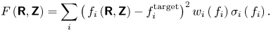 \begin{equation} F\left({\boldsymbol{\mathsf{R}}}, {\boldsymbol{\mathsf{Z}}}\right) = \sum_i \left(\,f_i\left({\boldsymbol{\mathsf{R}}}, {\boldsymbol{\mathsf{Z}}}\right) - f_i^{\mathrm{target}}\right)^{2} w_i\left(\,f_i\right) \sigma_i\left(\,f_i\right). \end{equation}
Here,  ${\boldsymbol{\mathsf{R}}}$ and ${\boldsymbol{\mathsf{Z}}}$ represent the arrays of the $R_{m,n}$ and $Z_{m,n}$ coefficients that define the boundary. The summation is over the different penalty functions, $f_i$, chosen by the user, each of which has a weight $w_i$, a target $f_i^{\mathrm {target}}$ and a function $\sigma _i$ which determines whether the penalty function is a target or a constraint. A target function tries to minimize $f_i - f_i^{\mathrm {target}}$ while a constraint only requires either $f_i < f_i^{\mathrm {target}}$ or $f_i > f_i^{\mathrm {target}}$.
The variation of the boundary coefficients  ${\boldsymbol{\mathsf{R}}}$ and ${\boldsymbol{\mathsf{Z}}}$ is performed through an optimization algorithm. For the resulting configuration shown here, Brent's algorithm is used (Brent Reference Brent2013). Additional details of this optimization technique can be found in Drevlak et al. (Reference Drevlak, Beidler, Geiger, Helander and Turkin2018) and Henneberg et al. (Reference Henneberg, Drevlak, Nührenberg, Beidler, Turkin, Loizu and Helander2019b), and results for similar optimizations of quasi-symmetric stellarators can be found in Ku et al. (Reference Ku, Garabedian, Lyon, Turnbull, Grossman, Mau and Zarnstorff2008).
The optimization for this new QHS configuration is an extension of a scheme that focused on improved energetic particle transport (Bader et al. Reference Bader, Drevlak, Anderson, Faber, Hegna, Likin, Schmitt and Talmadge2019). For the new optimization, multiple field periodicities and aspect ratios were considered. The best performing result presented here has four-field periods and an aspect ratio of 6.7. The metrics included in this optimization are the following:
(i) The deviation from quasi-symmetry, where the quantity to be minimized is defined as the energy in the non-symmetric modes normalized to some reference field, here the field on axis. In more detail, the configuration is converted into Boozer coordinates (Boozer Reference Boozer1981) and the magnitude of the magnetic field strength is represented in a discrete Fourier series with coefficients $B_{m,n}$. Then the quasi-symmetry deviation for a four-field-period device is calculated as
(2.3)where\begin{equation} P_{\textrm{QH}} = \left.\left( \sum_{n/m \neq 4} B_{m,n}^{2} \right) \right/ B_{0,0}^{2}, \end{equation}$B_{0,0}$ is the field on axis.
$B_{m,n}$. Then the quasi-symmetry deviation for a four-field-period device is calculated as
(2.3)where\begin{equation} P_{\textrm{QH}} = \left.\left( \sum_{n/m \neq 4} B_{m,n}^{2} \right) \right/ B_{0,0}^{2}, \end{equation}$B_{0,0}$ is the field on axis.(ii) The
$\varGamma _c$ metric is a proxy for energetic particle confinement (Nemov et al. Reference Nemov, Kasilov, Kernbichler and Leitold2008). In brief, this metric seeks to align contours of the second adiabatic invariant $J_\parallel$ with flux surfaces. Its viability in producing configurations with excellent energetic ion confinement was demonstrated in Bader et al. (Reference Bader, Drevlak, Anderson, Faber, Hegna, Likin, Schmitt and Talmadge2019).(iii) A magnetic well (Greene Reference Greene1997), where present, provides stability against interchange modes. Because finite-
$\beta$ effects in quasi-helical symmetry tend to deepen magnetic wells, it suffices to have a vacuum magnetic well of any strength. In this optimization, the vacuum well was required to exist at the magnetic axis, but was not optimized further beyond that.(iv) The rotational transform profile was chosen to avoid low-order rational surfaces, and to be sufficiently high above the
${\raise.3pt-\kern-5pt\iota} = 1$ surface to avoid a resonance when self-consistent, pressure-induced plasma current is added.(v) A target aspect ratio of 6.7 was chosen. In general, it is easier to satisfy most optimization targets at higher aspect ratios. Additionally, it is easier to generate coils that accurately reproduce the plasma boundary at high aspect ratios. However, smaller aspect ratios are desirable to reduce overall machine size, which is a major driving concern. The choice of 6.7 is a trade-off between good performance and reduction of device size.
(vi) The neoclassical transport metric
$\epsilon _{\mathrm {eff}}$ (Nemov et al. Reference Nemov, Kasilov, Kernbichler and Heyn1999) is required to remain below the value 0.01. In practice, adequate quasi-symmetry enforces this constraint automatically. In addition, proxies that attempt to align the maxima and minima values of the magnetic field strength on a field line were also employed in the optimizations. These proxies compute the contour of maximum (or minimum) magnetic field on a surface and seek to minimize the variance of the magnetic field strength on that contour.


The properties considered in the optimizer are all dimensionless quantities and are also independent of the choice of either major radius or magnetic field strength.
2.1 Configuration characteristics
A new optimized configuration, here termed the WISTELL-A configuration, has been generated through the optimization procedures described above. Figure 1 shows some of the properties of the configuration. Contours of the vacuum magnetic field strength on the boundary are shown in figure 1(a). The helical nature of the magnetic field strength, a feature of quasi-helical symmetry, is clearly seen. Figure 1(b) shows toroidal cuts of the boundary surface at toroidal angles 0,  ${\rm \pi} /8$ and ${\rm \pi} /4$, colloquially referred to as the ‘bean’, ‘teardrop’ and ‘triangle’ surfaces, respectively. Shown are both the vacuum boundary surfaces (red) and the surfaces with normalized plasma pressure $\beta = 0.94\,\%$. The surfaces with finite pressure are generated by a free boundary solution using coils and self-consistent bootstrap current. For finite- $\beta$ calculations throughout this work, the assumed profiles, given in terms of the normalized toroidal magnetic flux $s=\psi / \psi _{\textrm {LCFS}}$, were $T_e = T_i \propto (1-s)$, $N_e = N_i \propto (1-s^{5})$, $Z_{\textrm {eff}}=1$ and $P = P_e + P_i \propto (1 - s - s^{5} + s^{6})$. The procedure for generating finite- $\beta$ equilibria is described in § 4.3. The bootstrap current modifies the rotation transform. The finite-pressure boundary is somewhat smaller than the vacuum boundary.
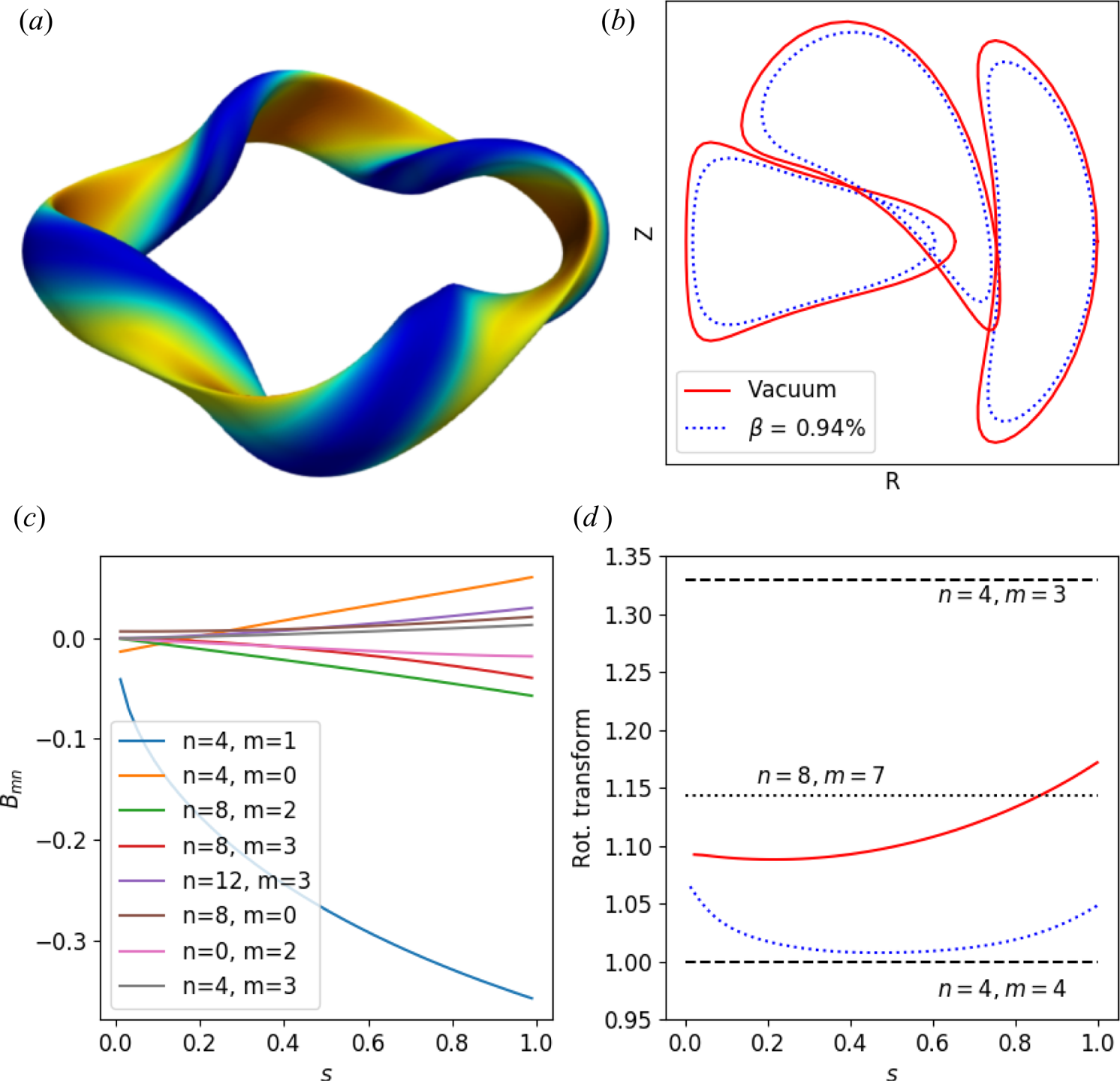
Figure 1. (a) Contours of the magnetic field strength on the boundary. (b) Boundary surfaces at toroidal cuts of toroidal angles 0,  ${\rm \pi} /8$ and ${\rm \pi} /4$ for the vacuum configuration (red) and a configuration with 0.94 % $\beta$ (blue dots). (c) The vacuum Boozer spectrum with the strengths of the eight most dominant modes as a function of normalized toroidal flux, $s$. (d) The vacuum rotational transform profile (red) and the rotational transform profile at 0.94 % $\beta$ (blue dots); important rational surfaces are plotted with dashed and dotted black lines.
Figure 1(c) shows the Boozer spectrum for the vacuum equilibrium where the  $n=0, m=0$ mode has been suppressed. The $n=4, m=1$ mode is dominant, which is expected for a four-period QHS equilibrium. The largest non-symmetric modes are the mirror mode at $n=4, m=0$ and the $n=8, m=3$ mode. Note that the $n=8, m=2$ mode has the same helicity as the dominant harmonic. Figure 1(d) shows the rotational transform profile both for vacuum and at $\beta = 0.94$ %. The dashed black lines represent the major low-order rational surfaces that should be avoided; these are the ${\raise.3pt-\kern-5pt\iota} = 1.0$ and ${\raise.3pt-\kern-5pt\iota} = 4/3$ surfaces. The configuration passes through the ${\raise.3pt-\kern-5pt\iota} = 8/7$ surface at the edge in the vacuum configuration. This vacuum surface can possibly be used to test island divertor features, which will be discussed in § 4.4. The blue dotted line in figure 1(d) represents the rotational transform profile at $\beta = 0.94$ %. As can be seen, the minimum of the rotational transform profile is just above the ${\raise.3pt-\kern-5pt\iota} = 1$ surface.
In addition, we note some features of the configuration used in the optimization. In figure 2, we show the neoclassical transport, as quantified by the  $\epsilon _{\mathrm {eff}}$ metric, the quasi-symmetry deviation, as described in (2.3), and the $\varGamma _c$ metric for vacuum configurations. In order to provide a baseline for comparison, we include the same quantities calculated for the HSX equilibrium (black). Helically Symmetric eXperiment has better values obtained for the quasi-symmetry metric, but slightly worse values for $\epsilon _{\mathrm {eff}}$ and $\varGamma _c$ over the majority of the minor radius. In addition to the optimized vacuum configuration, we also show the quantities for the vacuum fields produced by filamentary coils. The results here show that the configuration produced with coils does a very good job at reproducing the important qualities of the equilibrium.
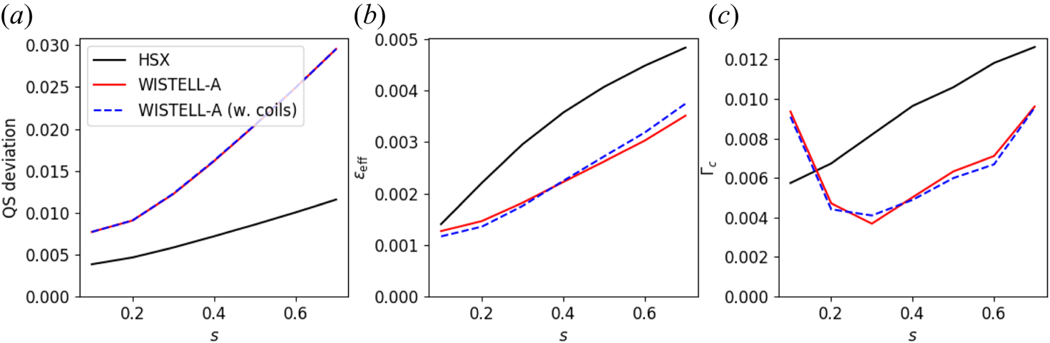
Figure 2. Values of the quasi-symmetry deviation (a),  $\epsilon _\mathrm {eff}$ (b) and $\varGamma _c$ (c) are plotted as a function of normalized toroidal flux $s$ for three configurations: the HSX configuration (black solid), the WISTELL-A configuration (red solid) and the WISTELL-A configuration as produced by coils (blue dashed).
3 Coil construction
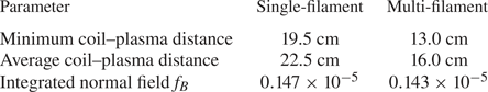
Coils to reproduce the vacuum boundary were produced by the FOCUS code (Zhu et al. Reference Zhu, Hudson, Song and Wan2018) using an initial coil set generated by the REGCOIL code (Landreman Reference Landreman2017). The FOCUS code targets the average normal field on the magnetic boundary (a quantity to minimize) and the minimal radius of curvature for the coils (a quantity to maximize). A representation of the coils is given in figure 3(a) along with the magnetic field magnitude on the boundary. In addition a Poincaré plot generated using Biot–Savart following of field lines produced by the filamentary magnetic coils is shown in figure 3(b). The results show that the internal surfaces are well formed without the presence of magnetic islands.

Figure 3. (a) A representation of coils for the WISTELL-A configuration. Internal to the coils is a representation of the magnetic field strength on the boundary as produced by the coils. (b) A Poincaré plot for surfaces produced by the coils represented in (a).
Of particular importance is the fact that the FOCUS code does not require a specified coil winding surface, and is therefore able to move the coils further from the plasma in regions where the reliability of reproducing the configuration is less sensitive to the coil position. The ability to optimize without being confined to a winding surface is a new capability within FOCUS that was not available for the coil sets designed for HSX and W7-X. Previous results showed that areas of low sensitivity can be calculated for stellarator equilibria using shape gradients (Landreman & Paul Reference Landreman and Paul2018). Fortuitously, these regions of low sensitivity are also the areas were divertor heat fluxes tend to exit the plasma (Bader et al. Reference Bader, Boozer, Hegna, Lazerson and Schmitt2017), allowing for the construction of a non-resonant divertor as described in § 4.4.
4 Performance evaluation
The performance of the configuration is evaluated in several topical areas. These include confinement of energetic particles evaluated by Monte Carlo analysis, turbulent transport evaluated by nonlinear Gene simulations (Jenko et al. Reference Jenko, Dorland, Kotschenreuther and Rogers2000), stability at finite pressure evaluated by COBRAVMEC (Sanchez, Hirshman & Ware Reference Sanchez, Hirshman and Ware2000) and an initial attempt at edge transport and divertor behaviour evaluated by EMC3-EIRENE (Feng et al. Reference Feng, Sardei, Kisslinger, Grigull, McCormick and Reiter2004).
4.1 Energetic particles
Energetic particle optimization was obtained in these configurations by targeting the  $\varGamma _c$ metric that seeks to align contours of the second adiabatic invariant $J_\parallel$ with flux surfaces. The calculation for $\varGamma _c$ is given in Nemov et al. (Reference Nemov, Kasilov, Kernbichler and Leitold2008, Eq. (61)) as
 \begin{equation} \varGamma_c = \frac{{\rm \pi}}{\sqrt{8}} \lim_{L_s \rightarrow \infty} \left( \int_0^{L_s} \frac{\textrm{d}s}{B} \right)^{-1} \left[ \int_1^{B_{\max}/B_{\min}} \textrm{d}b' \sum_{\mathrm{well}_j} \gamma_{cj}^{2} \frac{v \tau_{b,j}}{4 B_{\min} {b'}^{2}} \right], \end{equation}
where the electric field contribution is ignored. The arbitrary reference field  $B_0$ in Nemov et al. (Reference Nemov, Kasilov, Kernbichler and Leitold2008, Eq. (61)) is set to the minimum magnetic strength on the field line $B_{\min }$. The quantity $\gamma _c$ is
 \begin{equation} \gamma_c = \frac{2}{{\rm \pi}} \mathrm{arctan} \left( \frac{v_r}{v_\theta} \right). \end{equation}
Here,  $v_r$ is the bounce averaged radial drift and $v_\theta$ is the bounce averaged poloidal drift. The ratio $v_r/v_\theta$ is the key quantity to minimize. A method to calculate $v_r/v_\theta$ from geometrical quantities of the magnetic field line is described in Nemov et al. (Reference Nemov, Kasilov, Kernbichler and Leitold2008, Eq. (51)). The summation in (4.1) is taken over all the wells for a suitably long field line. In our case between 60 and 100 toroidal transits were used. The calculation considers trapping wells encountered by all possible trapped-particle pitch angles, with $b'$ representing a normalized value of the reflecting field. The bounce time for a particle in a specific magnetic well is given by $\tau _{b,j}$. The parameters $B_{\max }$ and $B_{\min }$ are the maximum and minimum magnetic field strength on the flux surface.
Previously, equilibria in ROSE were optimized by simultaneously minimizing  $\varGamma _c$ and the quasi-helical symmetry deviation. This resulted in configurations with very low collisionless particle losses (Bader et al. Reference Bader, Drevlak, Anderson, Faber, Hegna, Likin, Schmitt and Talmadge2019). However, calculations to assess energetic confinement used ideal, fixed boundary equilibria and did not include the effects of coils. For the following evaluation of the new configuration, collisionless energetic particle losses are calculated using the magnetic field structure produced from the filamentary coils presented in § 3.
To evaluate energetic particle transport, a scaling of the configuration to reactor-relevant parameters is necessary. Therefore, the transport of fusion-born alpha particles is examined in a configuration scaled to the ARIES-CS volume ( $450\ \textrm {m}^{3}$) and on-axis field strength (5.7 T). We choose a flux surface and distribute the alpha particles on the flux surface such that they properly resemble a distribution of alpha particles. The evaluation is done with the ANTS code (Drevlak et al. Reference Drevlak, Geiger, Helander and Turkin2014), which constructs a magnetic field grid in cylindrical coordinates. Therefore, ANTS is well suited to evaluate both the ideal equilibrium and the equilibrium produced by the filamentary coils. In both cases, 5000 particles are included in the evaluation for each flux surface for 200 ms, which corresponds to 2 alpha slowing down times at the core ARIES-CS density ( $n_e = 5 \times 10^{20}\ \textrm {m}^{-3}$) and temperature ( $T_e = 12\ \textrm {keV}$) and to 10 alpha slowing down times at the mid-radius density ( $n_e = 5 \times 10^{20}\ \textrm {m}^{-3}$) and temperature ( $T_e = 4\ \textrm {keV}$). Previous calculations indicated that 5000 particles per flux surface were sufficient for Monte Carlo statistical purposes (Bader et al. Reference Bader, Drevlak, Anderson, Faber, Hegna, Likin, Schmitt and Talmadge2019). These calculations only consider the vacuum fields, and improvements with finite pressure and plasma currents are left for future optimization studies. Similarly, calculations including collisional effects are left for future analyses.
The results for the energetic particle confinement are shown both with and without coils in figure 4. The confinement does deteriorate slightly with the presence of coils. Some particles are lost at  $s=0.2$, whereas in the ideal case, no particles are lost. The losses just outside the mid-radius, at $s=0.3$, increase from 1.2 % in the ideal case to 1.7 % in the configuration with coils. Also included in figure 4 are the results from the HSX configuration scaled to ARIES-CS volume and magnetic field. The finite ripple from the HSX coils produces significant alpha particle losses and at the ARIES-CS scale nearly all trapped particles are lost (approximately 25 % of the total particles). The poor performance of HSX agrees with previous results of alpha particle confinement by Nemov, Kasilov & Kernbichler (Reference Nemov, Kasilov and Kernbichler2014).
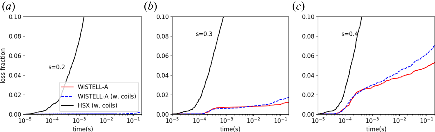
Figure 4. Collisionless alpha particle losses are plotted as a function of time for three flux surfaces corresponding to normalized toroidal fluxes of 0.2 (a), 0.3 (b) and 0.4 (c). Red is the ideal WISTELL-A configuration, blue dashed is the WISTELL-A configuration with coils and black is the HSX configuration. All configurations are scaled to the ARIES-CS volume and field.
The lost particles are shown as a function of starting pitch angle at  $s=0.4$ in figure 5. Here, the $x$ axis represents the field at which the particle reflects: $B_{\textrm {ref}} = E/\mu$, where $E$ and $\mu$ are the particle's energy and magnetic moment. Low values of $B_{\textrm {ref}}$ represent deeply trapped particles, and high values of $B_{\textrm {ref}}$ represent particles near the trapped–passing boundary. The trapped–passing boundary is indicated with a vertical dashed line. All passing particles are confined.
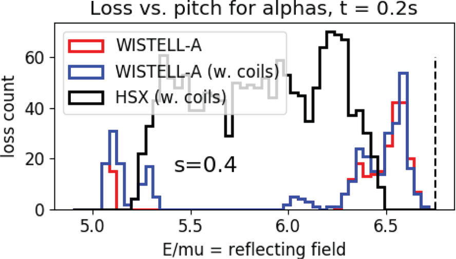
Figure 5. Alpha particle losses as a function of pitch angle for the ideal fixed boundary WISTELL-A configuration (red), the vacuum field from filamentary coils for WISTELL-A (blue) and the HSX configuration (black). The vertical dashed black line represents the trapped–passing boundary for the WISTELL-A configuration.
As is clear from the results in figure 5, most of the particle losses are from particles near the trapped–passing boundary. However, there are a few additional losses of deeply trapped particles, and from particles somewhat further from the trapped–passing boundary, at  $E/\mu \approx 6.0$. The results for a scaled version of HSX are also presented, showing particle losses for all trapped particle pitch angles.
4.2 Turbulent transport
Improving turbulent transport is a key area for stellarator research. Recent results from W7-X indicate turbulent transport determines the overall energy and particle confinement (Bozhenkov et al. Reference Bozhenkov, Kazakov, Ford, Beurskens, Alcusón, Alonso, Baldzuhn, Brandt, Brunner and Damm2020; Pablant et al. Reference Pablant, Langenberg, Alonso, Baldzuhn, Beidler, Bozhenkov, Burhenn, Brunner, Dinklage and Fuchert2020). The dominance of turbulent transport in optimized stellarators had also been previously shown for HSX plasmas (Canik et al. Reference Canik, Anderson, Anderson, Likin, Talmadge and Zhai2007). The configuration presented here is not explicitly optimized for turbulent transport. However, previous gyrokinetic calculations indicate that QHS configurations demonstrate enhanced nonlinear energy transfer properties over other optimized configurations (Plunk, Xanthopoulos & Helander Reference Plunk, Xanthopoulos and Helander2017; McKinney et al. Reference McKinney, Pueschel, Faber, Hegna, Talmadge, Anderson, Mynick and Xanthopoulos2019). It is anticipated that future iterations will include optimization of nonlinear turbulent energy transfer using a novel metric modelling turbulent energy transfer to stable modes (Hegna et al. Reference Hegna, Terry and Faber2018; Faber Reference Faber2020). Despite the lack of the turbulence metric in the optimization scheme, some aspects of the turbulence properties can be deduced from analysing the equilibrium.
Nonlinear flux-tube gyrokinetic calculations were performed to describe ion temperature gradient (ITG) turbulence at the  $s=0.5$ surface using the Gene code (Jenko et al. Reference Jenko, Dorland, Kotschenreuther and Rogers2000) for various values of the ion temperature scale length $a/L_{\textrm {Ti}}$ assuming adiabatic electrons. In figure 6, the heat flux in dimensionless gyro-Bohm units for WISTELL-A is compared to two other configurations, the HSX configuration, which has been well analysed for turbulent transport (Faber et al. Reference Faber, Pueschel, Proll, Xanthopoulos, Terry, Hegna, Weir, Likin and Talmadge2015; Pueschel et al. Reference Pueschel, Faber, Citrin, Hegna, Terry and Hatch2016; Faber et al. Reference Faber, Pueschel, Terry, Hegna and Roman2018; McKinney et al. Reference McKinney, Pueschel, Faber, Hegna, Talmadge, Anderson, Mynick and Xanthopoulos2019), and a third ‘turbulent reduced’ configuration, which was the result of a separate optimization calculation. The turbulence-reduced configuration is identical to the configuration in Bader et al. (Reference Bader, Drevlak, Anderson, Faber, Hegna, Likin, Schmitt and Talmadge2019) labelled ‘Opt. for QHS and $\varGamma _c$’. It possessed favourable energetic particle properties, but did not possess a vacuum magnetic well. Nevertheless, the turbulent properties of this configuration are of interest. The results show that WISTELL-A reduces turbulent heat flux relative to HSX in the regime of low ion temperature scale length. However, for $a/L_{\textrm {Ti}} \geq 2$, the heat flux is comparable to that of HSX. The turbulence-reduced configuration, on the other hand, demonstrates reduced heat flux across a range of $a/L_{\textrm {Ti}}$ and a notable reduction in heat flux from HSX and WISTELL-A at $a/L_{\textrm {Ti}} \geq 3$.
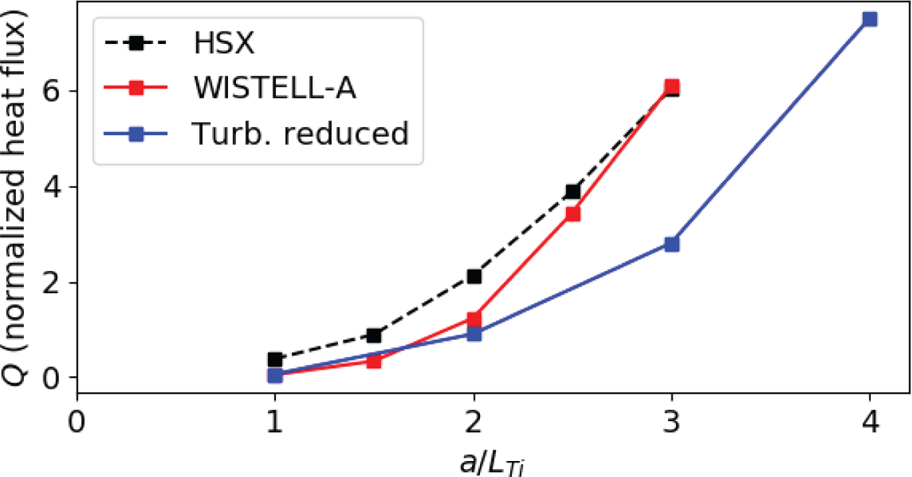
Figure 6. Turbulent heat flux in gyro-Bohm units at the  $s=0.5$ surface as a function of normalized ion temperature scale length $a/L_{\textrm {Ti}}$ for three different configurations: HSX (black dashed), WISTELL-A (red) and a turbulence-reduced configuration (blue).
Analysis of the turbulence at  $a/L_{\textrm {Ti}} = 3$ for each configuration indicates that the differences in the ion heat flux values at $s = 0.5$ are not associated with changes in the linear ITG instability spectrum. Figure 7 shows the heat flux in dimensionless gyro-Bohm units at $a/L_{\textrm {Ti}} = 3$ for each configuration as a function of $k_y\rho _s$. The HSX and WISTELL-A show similar heat flux spectra, with the flux peaking at $k_y\rho _s \approx 0.6$. The prominent feature in the WISTELL-A flux spectrum at $k_y\rho _s = 0.2$ has been previously observed and analysed in gyrokinetic simulations of HSX (Faber et al. Reference Faber, Pueschel, Proll, Xanthopoulos, Terry, Hegna, Weir, Likin and Talmadge2015, Reference Faber, Pueschel, Terry, Hegna and Roman2018) and while large in value, does not contribute substantially to the bulk of the heat flux. More strikingly, the bulk of the heat flux spectrum in the turbulence-reduced configuration is down-shifted in $k_y\rho _s$ from $k_y\rho _s \approx 0.6$ to $k_y\rho _s \approx 0.3$. The linear growth rate spectrum normalized by the ratio of the ion acoustic speed to the average minor radius as a function of $(k_x\rho _s,k_y\rho _s)$ for each configuration at $a/L_{\textrm {Ti}} = 3$ is shown in figure 8. Visual inspection of the growth rate spectra indicates there is little difference in the dominant linear instability between each configuration, and in fact the turbulence-reduced configuration (figure 8c) has larger growth rates than either HSX or WISTELL-A. This observation is supported more directly by using the eigenmode data from figure 8 in a quasi-linear heat flux calculation using the model described in Pueschel et al. (Reference Pueschel, Faber, Citrin, Hegna, Terry and Hatch2016, Eq. (2)), which is reproduced here:
 \begin{align} \left.\begin{array}{c}\displaystyle Q_{\textrm{QL}}= \frac{a}{L_{\textrm{Ti}}}\mathcal{C}\sum_{k_x,k_y}\frac{w_i(k_x,k_y) \gamma(k_x,k_y)}{\langle k_{i,\perp}^{2}(k_x,k_y)\rangle},\\ \displaystyle \langle k_\perp^{2}(k_x,k_y) \rangle= \frac{\int \mathrm{d}z \sqrt{g(z)} \varPhi^{2}(k_x,k_y,z) k_\perp^{2}(k_x,k_y,z)}{\int \mathrm{d}z \sqrt{g(z)} \varPhi^{2}(k_x,k_y,z)}.\end{array}\right\} \end{align}
The linear growth rate  $\gamma (k_x,k_y)$ is calculated from a linear Gene simulation at normalized perpendicular wavenumber $(k_x,k_y)$ and produces an eigenmode $\varPhi (k_x,k_y,z)$, where $z$ is the field-line-following coordinate. The Jacobian along the field line is given by $\sqrt {g(z)}$ and each contribution to the sum is weighted by $w_i = \tilde {Q}_i/\tilde {n}_i^{2}$, where $\tilde {Q}_i$ and $\tilde {n}_i$ are the calculated linear gyrokinetic heat flux and density perturbations from Gene. The normalizing coefficient $\mathcal {C}$ is fit to a nonlinear gyrokinetic heat flux calculation and $a/L_{\textrm {Ti}}$ is the normalized temperature gradient; only ratios of $Q_{\textrm {QL}}$ will be considered here to avoid model ambiguity. The quasi-linear calculation predicts that the heat flux for the turbulence-reduced configuration should actually be larger than that for HSX at $a/L_{\textrm {Ti}}=3$ by a factor of approximately 1.1. This does not agree with the nonlinear gyrokinetic heat fluxes shown in figure 6. The discrepancy between the linear growth rates and the full nonlinear heat flux is consistent with trends found in McKinney et al. (Reference McKinney, Pueschel, Faber, Hegna, Talmadge, Anderson, Mynick and Xanthopoulos2019). The results presented here also indicate that linear growth rates can be a misleading indicator for stellarator turbulence and turbulent transport. Furthermore, these results suggest that the turbulence-reduced configuration possesses enhanced turbulence saturation mechanisms.
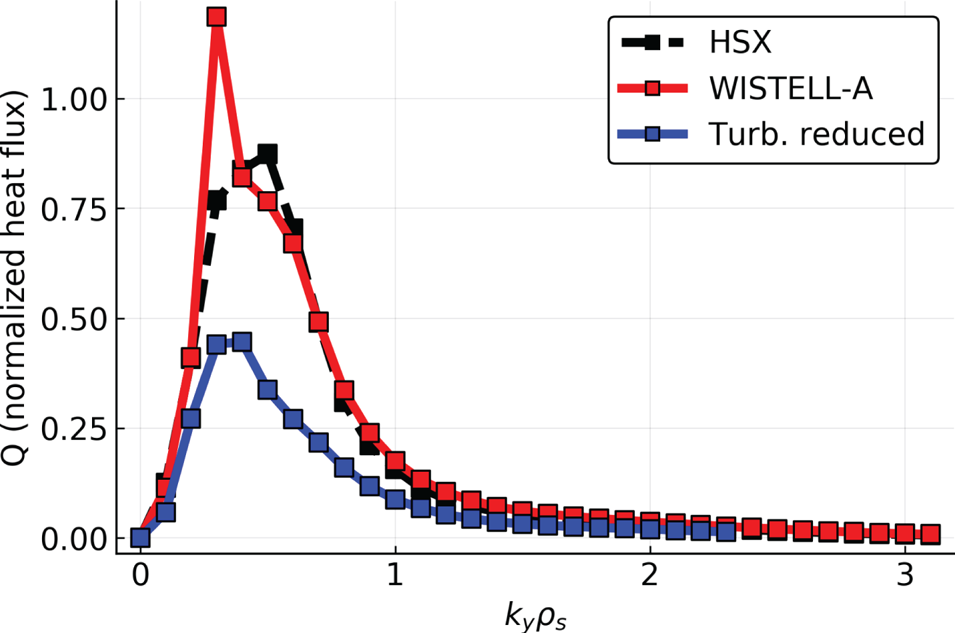
Figure 7. Turbulent heat flux spectrum in gyro-Bohm units at  $a/L_{\textrm {Ti}}=3$ from figure 6 as a function of normalized binormal wavenumber $k_y\rho _s$ for HSX (black dashed), WISTELL-A (red) and a turbulence-reduced configuration (blue).
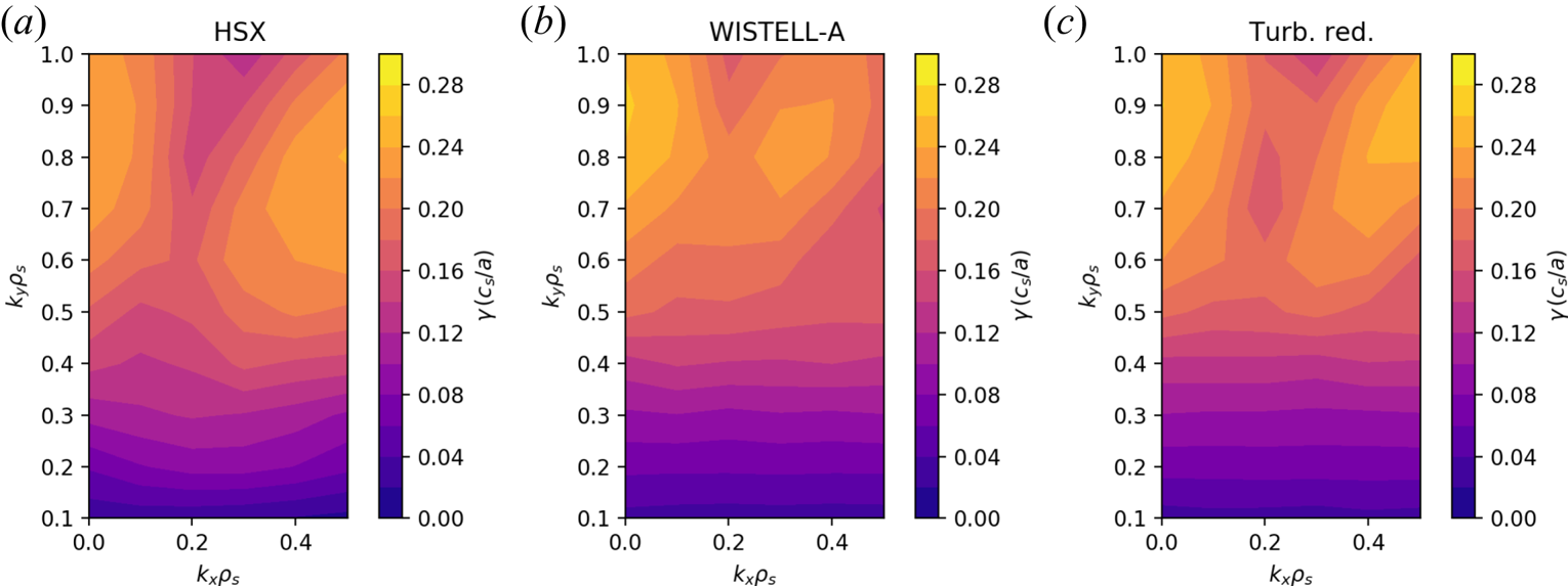
Figure 8. Ion temperature gradient growth rate spectrum in units of  $c_s/a$ with $a/L_{\textrm {Ti}} = 3$ as a function of normalized radial wavenumber $k_x\rho _s$ and normalized binormal wavenumber $k_y\rho _s$: (a) HSX, (b) WISTELL-A and (c) turbulence-reduced configurations.
To make a preliminary assessment of the turbulence saturation characteristics, the turbulence saturation theory from Hegna et al. (Reference Hegna, Terry and Faber2018) is applied. A crucial aspect of this theory is the supposition that the dominant nonlinear physics involves energy transfer from unstable to damped eigenmodes at comparable wavenumbers. This is accomplished through a three-wave interaction quantified by a triplet correlation lifetime between unstable and stable ITG modes as defined in Hegna et al. (Reference Hegna, Terry and Faber2018, Eq. (104)) by
 \begin{equation} \tau_{\textrm{pst}}(\boldsymbol{k},\boldsymbol{k}') = \frac{-\mathrm{i}}{\omega_t(\boldsymbol{k}'') + \omega_s(\boldsymbol{k}') - \omega^{\ast}_p(\boldsymbol{k})};\quad \boldsymbol{k} -\boldsymbol{k}' = \boldsymbol{k}'', \end{equation}
where  $\omega (\boldsymbol {k})$ is the normalized complex linear ITG frequency at normalized wavenumber $\boldsymbol {k} = (k_x\rho _s,k_y\rho _s)$. Large values of the triplet lifetimes suggest energy can be very effectively transferred out of turbulent-transport-inducing instabilities into damped eigenmodes that either dissipate energy or transfer it back to the bulk distribution function. High values of $\tau _{\textrm {pst}}$ correspond to lowered turbulent fluctuation levels and correspondingly reduced turbulent transport. In Hegna et al. (Reference Hegna, Terry and Faber2018), the dominant saturation mechanism was shown to be energy transfer to stable modes through non-zonal, marginally stable drift waves. As such, the analysis presented here focuses on assessing the energy transfer through non-zonal modes as opposed to energy transfer through zonal flows, which is shown to be the dominant saturation mechanism in tokamaks (Terry et al. Reference Terry, Faber, Hegna, Mirnov, Pueschel and Whelan2018), the NCSX stellarator (Hegna et al. Reference Hegna, Terry and Faber2018; McKinney et al. Reference McKinney, Pueschel, Faber, Hegna, Talmadge, Anderson, Mynick and Xanthopoulos2019) and the W7-X stellarator (Plunk et al. Reference Plunk, Xanthopoulos and Helander2017).
In figure 9, the triplet correlation lifetimes are shown for the HSX and the turbulence optimized configuration. Importantly, the turbulence-reduced configuration shows larger triplet correlation lifetimes in the region  $k_y\rho _s \lesssim 0.6$ compared to HSX, where the larger correlation lifetimes are observed at higher $k_y\rho _s$. This is an important difference, as instabilities at larger scales (smaller $|\boldsymbol {k}_\perp |$) can more easily contribute to turbulent transport. Thus, larger triplet correlation lifetimes at smaller $k_y\rho _s$ where at least one unstable and one stable mode are involved suggest energy is being transferred more efficiently from the modes driving the fluctuation spectrum to dissipation and thus lowering the contribution to turbulent transport at that
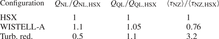
  $k_y\rho _s$. This may be contributing to both the decrease in overall transport in figure 6 and the down-shift in heat flux spectrum in figure 7 between HSX and the turbulence-reduced configuration. The connections between nonlinear turbulent heat flux, quasi-linear turbulent heat flux and the triplet correlation lifetimes are summarized in table 1. The triplet correlation lifetimes for each configuration are quantified by computing a spectral average defined as
 \begin{equation} \langle \tau_{\textrm{NZ}} \rangle = \sum_{k_x,k_y} \mathcal{S}_{G}(k_x,k_y) \textrm{Re}(\tau_{\textrm{NZ}}(k_x,k_y)). \end{equation}
The weighting factor  $\mathcal {S}(k_x,k_y)$ is a turbulent fluctuation spectrum computed from a characteristic nonlinear gyrokinetic simulation that preferentially weights low $|\boldsymbol {k}_\perp |$ contributions to provide consistency with the nonlinear simulations. The decrease in nonlinear flux between HSX and the turbulence-reduced configuration by a factor of two correlates with an increase in triplet correlation lifetimes by more than a factor of three, while the increase in nonlinear flux between WISTELL-A and HSX correlates with a decrease in triplet correlation lifetimes. This will be explored in more detail in future work. However, the result presented here already indicates that QHS configurations with lower ITG-driven transport can be obtained which are consistent with excellent energetic ion confinement and reduced neoclassical transport.
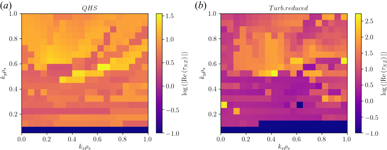
Figure 9. Triplet correlation lifetimes on a log scale as a function of  $\boldsymbol {k}$ for (a) HSX and (b) the turbulence-reduced configuration for $a/L_{Ti}=3$. The value shown at any particular $\boldsymbol {k}$ is the calculation of $\tau _{\textrm {pst}}$ as defined by (4.4a,b) where $p$ is an unstable mode at that $\boldsymbol {k}$ and $s$ is a stable mode at whatever wavenumber $\boldsymbol {k}'$ such that $\textrm {Re}(\tau _{pst}(\boldsymbol {k},\boldsymbol {k}'))$ is maximized by a third mode $t$, which can be unstable or stable. The triplet correlation lifetime value has been weighted by a fluctuation energy spectrum obtained from gyrokinetic calculations which emphasize triplet lifetimes involving energy-containing scales. The dark values on the plot correspond to regions either where no instability is observed, such as at $k_y\rho _{s} = 0.05$ in both plots, or where the triplet correlation lifetime is almost purely imaginary.
Table 1. Values of nonlinear gyrokinetic heat flux, quasi-linear heat flux and spectral averaged triplet correlation lifetimes at  $a/L_{\textrm {Ti}} = 3$ for the three configurations. All values have been normalized to the corresponding HSX value.
4.3 Magnetohydrodynamic stability
The MHD properties of quasi-helical stellarators (Nührenberg & Zille Reference Nührenberg and Zille1988) are somewhat distinct from those of other classes of optimized stellarators. The relatively reduced connection length (the distance along the field line between  $B_{\max }$ and $B_{\min }$) implies that quasi-helical stellarators have reduced banana widths, reduced orbit drifts for passing particles (Talmadge et al. Reference Talmadge, Sakaguchi, Anderson, Anderson and Almagri2001), smaller Pfrisch–Schlüter (Boozer Reference Boozer1981; Schmitt, Talmadge & Anderson Reference Schmitt, Talmadge and Anderson2013) and bootstrap currents (Boozer & Gardner Reference Boozer and Gardner1990; Schmitt et al. Reference Schmitt, Talmadge, Anderson and Hanson2014) and reduced Shafranov shift compared to an equivalent sized tokamak for the same parameters. This is quantified by the ‘effective’ rotational transform ${\raise.3pt-\kern-5pt\iota} _{\textrm {eff}} = ({\raise.3pt-\kern-5pt\iota} - N)$, where $N$ is the periodicity of the stellarator. Moreover, the bootstrap current in a quasi-helical stellarator is in the opposite direction relative to what occurs in a tokamak. This has the consequence of reducing the value of ${\raise.3pt-\kern-5pt\iota}$ with rising plasma pressure and producing negative $\textrm {d}{\raise.3pt-\kern-5pt\iota} /\textrm {d}s$ in the core region. Negative values of $\textrm {d}{\raise.3pt-\kern-5pt\iota} /\textrm {d}s$ can have beneficial effects for both ideal ballooning (Hegna & Hudson Reference Hegna and Hudson2001) and magnetic island physics (Hegna & Callen Reference Hegna and Callen1994).
In the following, the MHD stability properties are evaluated using local ideal MHD stability criteria. Local pressure-driven instabilities are evaluated using ideal MHD interchange ( $k{||} = 0$) and ballooning ( $k_{||} \neq 0$) stability calculations.
The only stability quantity constrained in the ROSE optimization is the magnetic well depth as described by  $\textrm {d}^{2}V/\textrm {d}\varPhi ^{2}$, the second derivative of volume with respect to toroidal flux, at the magnetic axis for the vacuum equilibrium. A magnetic well ( $V'' < 0$) is stabilizing to interchange instability. The magnetic well depth at points away from the magnetic axis was not explicitly optimized for, but can be quantified with
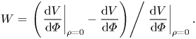 \begin{equation} W = \left.\left(\left.\frac{\textrm{d}V}{\textrm{d}\varPhi}\right|_{\rho=0} - \frac{\textrm{d}V}{\textrm{d}\varPhi}\right)\right/\left. \frac{\textrm{d}V}{\textrm{d}\varPhi}\right|_{\rho=0} . \end{equation}
The magnetic hill/well is a measure of the flux surface averaged field line curvature and a crucial quantity in evaluating the interchange stability properties of a magnetic configuration. In the following, a more comprehensive test of ideal MHD interchange stability is provided by an evaluation of the Mercier criterion. The strength of the magnetic hill/well is a prominent element in this evaluation.
For calculations including finite pressure, it is necessary to choose a machine size and field strength along with density and temperature profiles. For these calculations we assume the machine size as laid out in appendix A, with major radius  $R = 2\ \textrm {m}$ and axis magnetic field $B_0 = 2.5$ T. A pressure profile is assumed where temperature is linear in normalized flux, $T = T_0(1-s)$, and the density profile is broad, $n = n_0(1 - s^{5})$. Here, $T_0$ and $n_0$ represent the temperature and density at the magnetic axis, respectively. The pressure profiles as a function of normalized flux are given in figure 10(a). The pressure was varied by varying $T_0$ at fixed $n_0 = 0.9 \times 10^{20}\ \textrm {m}^{-3}$, with $T_0$ ranging from 1.3 to 3.5 keV. The free-boundary equilibrium was calculated with VMEC using the vacuum magnetic field given by the filamentary coils described in § 3. The self-consistent bootstrap current profiles are calculated using SFINCS (Landreman et al. Reference Landreman, Smith, Mollén and Helander2014) in an iterative loop with the VMEC equilibrium. In the neoclassical calculations, a pure plasma with $T_e = T_i$ was assumed, and the bootstrap current was calculated at the ambipolar radial electric field and is shown in figure 11. An iterative optimization scheme was used to solve for the toroidal current density $\textrm {d}I/\textrm {d}s$:
 \begin{equation} \frac{\textrm{d}I}{\textrm{d}s} = - \frac{\mu_0 I}{ \langle B_i^{2} \rangle }\frac{\textrm{d}p}{\textrm{d}s} + 2{\rm \pi} \frac{\textrm{d}\psi}{\textrm{d}s}\frac{\langle j_{||} B \rangle}{\langle B_i^{2} \rangle }. \end{equation}
Figure 10. (a) The pressure profiles versus normalized flux  $s$ for several values of volume-average $\beta$. The effects of finite $\beta$ are shown for the radial profiles (in $s$) of (b) the rotational transform ( ${\raise.3pt-\kern-5pt\iota} \equiv \iota / 2{\rm \pi}$), (c) the magnetic well depth and (d) the Mercier stability criterion. Positive values indicate Mercier stability. (Inset shows more detail for $0.4 < s < 1.0$.) Vacuum quantities for the rotational transform and well depth are shown (dashed lines).

Figure 11. The bootstrap current profiles versus normalized flux  $s$ for the same values of volume-average $\beta$ as in figure 10.
Calculating the toroidal current density and bootstrap current in this way ensures that the effects of all equilibrium currents generated by the plasma (diamagnetic, Pfirsch–Schlüter and bootstrap) are included in the magnetic field of the equilibrium. This equilibrium represents the plasma configuration after the current profile has relaxed to its steady-state value via current diffusion (with temperature and density profiles assumed stationary in time). The rotational transform profiles from the VMEC equilibria evaluated for several different pressures are shown in figure 10(b).
As noted previously, the bootstrap current tends to lower the value of  ${\raise.3pt-\kern-5pt\iota}$ and produce reversed magnetic shear in the core. As seen in figure 10(b), the rotational transform profile crosses ${\raise.3pt-\kern-5pt\iota} =1$ around $s \approx 0.5$ when the normalized pressure $\beta \approx 1\,\%$. Unless compensated for, this potentially sets an operational limit for this configuration.
With finite- $\beta$ equilibria, relevant stability metrics can be calculated. The well depths, as given by (4.6) are shown in figure 10(c). As seen in the figure, the vacuum configuration has a magnetic well, and the well depth gets larger as the pressure increases. Noting $V''$ is related to the derivative of $W$, the peak in the well depth indicates the radial location at which the configuration changes from having a stabilizing magnetic well to an unstable magnetic hill. This radial location increases with $\beta$; however, a magnetic hill region remains near the plasma edge at all values of $\beta$ explored here.
The Mercier criterion is given by the sum (Bauer, Betancourt & Garabedian Reference Bauer, Betancourt and Garabedian1984; Carreras et al. Reference Carreras, Dominguez, Garcia, Lynch, Lyon, Cary, Hanson and Navarro1988)
 \begin{equation} D_{\textrm{Merc}} = D_S + D_W + D_I + D_G \geq 0, \end{equation}
where the individual terms in (4.8) represent contributions (stabilizing or destabilizing) from the shear, magnetic well, current and geodesic curvature and are given by the following:
 \begin{gather*} D_S = \frac{s}{{\raise.3pt-\kern-5pt\iota}^{2} {\rm \pi}^{2}} \frac{\left(\varPsi'' \varPhi'\right)^{2}}{4}, \\ D_W = \frac{s}{{\raise.3pt-\kern-5pt\iota}^{2} {\rm \pi}^{2}} \int \int {g\,\textrm{d}\theta \,\textrm{d}\zeta \frac{B^{2}}{g^{\textrm{ss}}} \frac{\textrm{d}p}{\textrm{d}s}} \times \left(V'' - \frac{\textrm{d}p}{\textrm{d}s}\int\int{g \frac{\textrm{d}\theta \,\textrm{d}\zeta}{B^{2}}} \right),\\ D_I = \frac{s}{{\raise.3pt-\kern-5pt\iota}^{2} {\rm \pi}^{2}}\left[\int \int{g \,\textrm{d}\theta \,\textrm{d}\zeta \frac{B^{2}}{g^{\textrm{ss}}}\varPsi'' I'} - \left(\varPsi'' \varPhi' \right) \int\int{g \,\textrm{d}\theta \, \textrm{d}\zeta \frac{\left(\boldsymbol{J}\boldsymbol{\cdot}\boldsymbol{B}\right)}{g^{\textrm{ss}}}} \right], \\ D_G = \frac{s}{{\raise.3pt-\kern-5pt\iota}^{2} {\rm \pi}^{2}}\left[ \left( \int \int{g \,\textrm{d}\theta \,\textrm{d}\zeta \frac{\left(\boldsymbol{J}\boldsymbol{\cdot}\boldsymbol{B}\right)}{g^{\textrm{ss}}}} \right)^{2} - \left(\int \int{g \,\textrm{d}\theta \,\textrm{d}\zeta \frac{\left(\boldsymbol{J} \boldsymbol{\cdot}\boldsymbol{B}\right)^{2}}{g^{\textrm{ss}} B^{2}} }\right)\left(\int \int { g \,\textrm{d}\theta \,\textrm{d}\zeta \frac{B^{2}}{g^{\textrm{ss}}}} \right) \right]. \end{gather*}
 In the above expressions,  $\varPhi$ and $\varPsi$ are the toroidal and poloidal magnetic fluxes, $g$ is the Jacobian, $p$ is the pressure, $I$ is the net toroidal current enclosed within a magnetic surface and the metric element $g^{\textrm {ss}} = |\boldsymbol {\nabla }s|^{2}$.
Figure 10(d) shows the Mercier stability criterion as given by (4.8) and evaluated by VMEC. All configurations are Mercier stable ( $D_{\textrm {Merc}} > 0$) for $s \lesssim 0.6$. Calculations of ballooning stability were obtained with COBRAVMEC (Sanchez et al. Reference Sanchez, Hirshman and Ware2000) and are shown in figure 12. The configuration is stable to ballooning modes up to values of $\beta \leq 1.2\,\%$. Ballooning stability is violated at higher values of $\beta$ with the specified pressure profile shape. The region where ballooning instability tends to occur first is near $s \approx 0.7$. Higher critical $\beta$ values for ideal ballooning instability can be obtained by tuning the pressure profile. This will be pursued in future work.

Figure 12. (a) The radial profiles of the growth rates, as calculated by COBRAVMEC for various values of normalized pressure  $\beta$. Negative (positive) growth rates indicate stability (instability). Configurations that are stable for all radial positions are plotted as solid lines. Configurations are plotted as dashed lines if they are unstable at any radial position. (b) The value of the growth rate for the most unstable ballooning mode is shown as a function of normalized pressure $\beta$. The configuration at $\beta =1.16\,\%$ is stable to ballooning modes, while at $\beta =1.28$, the configuration becomes unstable with positive growth rates first appearing near $s \approx 0.7$.
The configuration presented here was optimized for quasi-helical symmetry, energetic particle confinement, neoclassical confinement and stability near the axis. The effects of finite plasma pressure and bootstrap current on the equilibrium were not considered, and finite- $\beta$ stability properties were not included as targets in the optimization. As a consequence, this configuration has only modest MHD stability limits. It is anticipated that the stability properties can be improved through optimization using equilibrium with finite $\beta$ and bootstrap current along with ideal MHD Mercier and ballooning stability evaluations. However, there is little evidence to support the notion that MHD stability provides any rigorous limit for stellarator operation (Weller et al. Reference Weller, Anton, Geiger, Hirsch, Jaenicke, Werner, Nührenberg, Sallander and Spong2001).
4.4 Divertor
Divertors for quasi-symmetric stellarators require either resilience to changes in the plasma current and pressure profiles or active control mechanisms to ensure proper function of a resonant divertor, often referred to as an island divertor, from startup to the operational point (König et al. Reference König, Grigull, McCormick, Feng, Kisslinger, Komori, Masuzaki, Matsuoka, Obiki and Ohyabu2002). Properties for non-resonant divertors have been explored both theoretically and numerically (Bader et al. Reference Bader, Boozer, Hegna, Lazerson and Schmitt2017, Reference Bader, Hegna, Cianciosa and Hartwell2018; Boozer & Punjabi Reference Boozer and Punjabi2018). In this section we present a methodology for constructing such a divertor, and provide a first attempt at what a non-resonant divertor could look like for a QHS stellarator.
As with the section on MHD stability, for this analysis we choose the machine size laid out in appendix A, with input power of 2 MW distributed evenly between ions and electrons. The methodology for constructing the divertor is to begin with a wall at some uniform distance from the last closed flux surface. A field line diffusion model can then be used to calculate the strike positions on the wall (Strumberger Reference Strumberger1992; Bader et al. Reference Bader, Boozer, Hegna, Lazerson and Schmitt2017). The model works by distributing field lines uniformly on good internal flux surfaces. Points are followed along the field line but given a random perpendicular displacement in accordance with a specified diffusion parameter. The ‘diffusive’ field lines eventually leave the confined region and terminate on the wall. These exiting field lines are always seen to exit the plasma in regions of high curvature of the last closed flux surface (Strumberger Reference Strumberger1992; Bader et al. Reference Bader, Boozer, Hegna, Lazerson and Schmitt2017).
As noted above, a benefit of the FOCUS code is that it allows the coils to expand away from the plasma in regions where they are not required to be close to the plasma. Fortuitously, the regions of high curvature where strike lines exit are also regions where coil expansion is possible. Therefore, a method for divertor construction is to adjust the uniform wall so it is expanded in these regions. This allows for both longer connection lengths between the plasma and the wall and some degree of divertor closure, allowing for access to high neutral pressure.
An initial attempt at such a construction is shown in figure 13. Here four plots of the divertor structure at toroidal values of  $\phi = 0^{\circ }$, $15^{\circ }$, $30^{\circ }$ and $45^{\circ }$ are shown. In addition, an EMC3-EIRENE simulation was carried out using operating parameters for the upgraded scenario. The calculation from EMC3-EIRENE indicates that the heat flux is concentrated in specific areas toroidally and poloidally near $\phi = 30^{\circ }$. A three-dimensional representation of the divertor design is shown in figure 14.

Figure 13. A representation of a non-resonant divertor concept for the WISTELL-A device. Plots correspond to four toroidal positions at  $\phi = 0^{\circ }$, $15^{\circ }$, $30^{\circ }$ and $45^{\circ }$. The wall (solid blue) is expanded near regions of peak heat flux. The heat flux is calculated by EMC3-EIRENE and shown in colour.
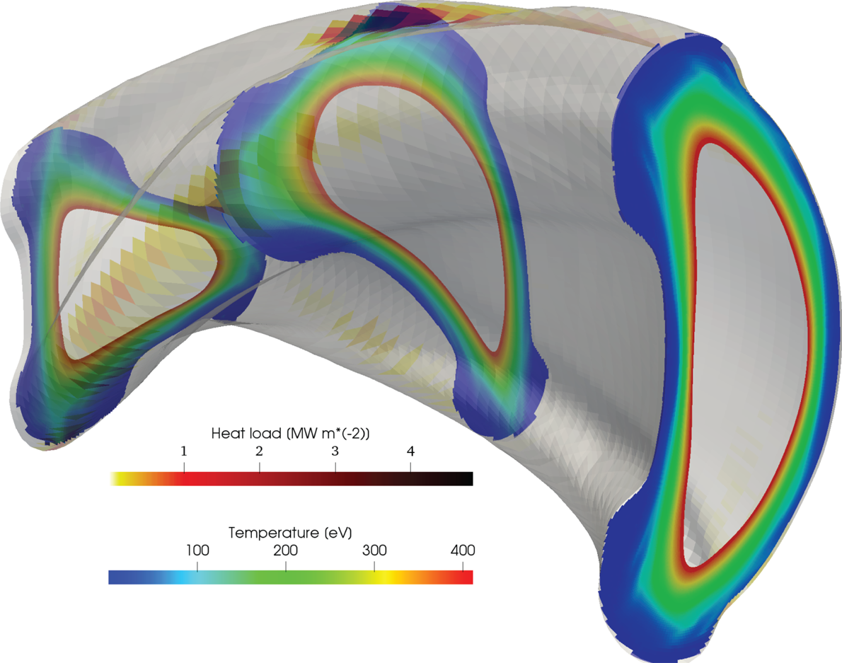
Figure 14. A three-dimensional representation of a non-resonant divertor concept for the WISTELL-A device. The grey outer surface represents the wall. Temperature contours from EMC3-EIRENE are presented at  $\phi = 0^{\circ }$, $22.5^{\circ }$ and $45^{\circ }$, and the heat flux on the wall is also represented on the boundary.
Future iterations of the divertor structure design are necessary in order to smooth the heat flux deposition. The results presented here are therefore meant to indicate a first attempt at how divertor design could proceed and not indicative of a final design.
In addition, the configuration will have access to island divertor experiments by exploiting the  $n=8,m=7$ resonance. However, due to the presence of self-generated plasma currents in quasi-symmetric equilibria, ensuring the island position is maintained throughout the discharge to the operating point requires some external control, whether by auxiliary coils or current drive. Designing such operational scenarios is beyond the scope of this current work.
5 Conclusion
A new optimized QHS stellarator is developed that has a number of desirable features including improved energetic ion confinement, low neoclassical transport and non-resonant divertor capability. Additionally, preliminary calculations indicate that QHS configurations with reduced turbulent transport exist that are consistent with these favourable properties. The new configuration is made possible through the simultaneous improvements in optimization (ROSE) and coil (FOCUS) tools as well as advances in physics understanding. Stellarator optimization is a rapidly developing field with new advancements in physics metrics, equilibrium solutions and optimization algorithms occurring at an impressive pace. Individual optimized equilibria represent markers of where progress is at a given point in time. They highlight recent advancements and provide benchmarks for testing further optimizations.
A particularly significant advance is the development of configurations with excellent energetic particle confinement. Importantly, this improved energetic ion confinement is realized in the presence of external magnetic fields generated from filamentary coils. These improvements were only possible due to recent improvements in stellarator optimization.
A relatively new element in stellarator optimization is targeting reduced turbulent transport. In addition to the configuration presented here, another turbulence-reduced configuration has been identified. Nonlinear gyrokinetic simulations of ITG turbulence demonstrate that this configuration has improved normalized values of heat flux relative to that predicted in HSX for all values of ITG drive. Interestingly, improvements in turbulent transport are not correlated to significant changes to the linear stability properties. Rather, there are indications that the improved turbulent transport is related to changes in the nonlinear energy transfer physics.
Quasi-helically symmetric stellarators have a number of intrinsic advantages when compared to other optimized stellarators. The reduced connection lengths of quasi-helical relative to quasi-axisymmetric implies they have smaller banana widths, Shafranov shifts and plasma-generated currents. However, MHD effects need to be accounted for in comprehensive stellarator optimization. Only modest attempts were made to improve the MHD properties of this new configuration. Nevertheless, configurations with magnetic wells throughout the core confinement regime are realized with ballooning instability onset at  $\beta$ of a few percent. There is reason to believe this property can be improved.
There is a need for a viable divertor option for stellarators with finite bootstrap current. Initial calculations show that non-resonant divertors, which do not rely on a low-order resonance at the edge, may be a possible solution. The complex interactions between edge plasma, impurities, neutral gas and plasma boundary surfaces in a stochastic edge are only accessible numerically with the EMC3-EIRENE code. Validation of this code in different edge scenarios in experiments with relevant geometries and conditions is necessary to predict the functionality of next-step experiments.
A final advantage of new equilibria is that they can be the foundation for new experimental designs. In appendix A, a conception of a midscale QHS stellarator is given.
Acknowledgements
This work was supported by the University of Wisconsin, UW2020-135AAD3116, and US Department of energy grants DE-FG02-93ER54222 and DE-FG02-99ER54546. B.J.F. is supported by the US Department of Energy Fusion Energy Sciences Postdoctoral Research Program administered by the Oak Ridge Institute for Science and Education (ORISE) for the DOE. ORISE is managed by Oak Ridge Associated Universities (ORAU) under DOE contract number DE-SC0014664. All opinions expressed in this paper are the authors’ and do not necessarily reflect the policies and views of DOE, ORAU or ORISE. This research used resources of the National Energy Research Scientific Computing Center (NERSC), a US Department of Energy Office of Science User Facility operated under contract no. DE-AC02-05CH11231.
Editor Per Helander thanks the referees for their advice in evaluating this article.
Declaration of interests
The authors report no conflict of interest.
Appendix A
This appendix details a possible realization of the new configuration as a midscale experiment. Such an experiment could significantly advance the quasi-symmetric concept and retire some of the risks related to energetic particle transport, turbulent transport and divertor operation in quasi-symmetry. Importantly, neither the configuration itself nor the parameters given here are meant to represent a final machine design. It is expected that many further optimizations will take place to improve the physics basis. Rather, the appendix here is meant to indicate what rough parameter scales are necessary to experimentally measure the relevant physics.
A zero-dimensional analysis was carried out in order to determine a target equilibrium for a realization of the WISTELL-A configuration for a midscale experiment. Details are presented in table 2. The major size and cost drivers are the magnetic field strength and the minor radius. In addition the operation is split into two phases, an initial operational phase at half field (1.25 T) and a full operational phase at 2.5 T. The magnetic field strength is chosen to take advantage of electron cyclotron heating (ECH) from commercially available 70 GHz gyrotrons at the second harmonic in the initial phase. In the full operational phase, the 70 GHz gyrotrons can be used at the fundamental O-mode harmonic, or 140 GHz gyrotrons can be used to heat at the second harmonic. The choice of gyrotron frequency sets the density cutoff, the maximum operational density for ECH plasmas. The cutoff density is  $\epsilon _0 m_e \omega ^{2} / e^{2}$, where $\epsilon _0$ is the permittivity of free space, $m_e$ is the electron mass, $e$ is the fundamental charge and $\omega$ is the angular frequency of the launched wave. For 70 GHz gyrotrons the cutoff is ${\sim }0.6 \times 10^{20}\ \textrm {m}^{-3}$. For 140 GHz gyrotrons the cutoff is ${\sim }2.4 \times 10^{20}\ \textrm {m}^{-3}$. The Sudo density limit for 1 MW absorbed power is $9.0 \times 10^{20}\ \textrm {m}^{-3}$ (Sudo et al. Reference Sudo, Takeiri, Zushi, Sano, Itoh, Kondo and Iiyoshi1990).
Table 2. Parameters and derived quantities (using zero-dimensional analysis) for the WISTELL-A stellarator for the initial operational phase and three scenarios for the full operational phase.
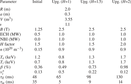
The confinement time  $\tau _E$ (in ms) is given by the ISS04 empirical scaling law (Yamada et al. Reference Yamada, Harris, Dinklage, Ascasibar, Sano, Okamura, Talmadge, Stroth, Kus and Murakami2005):
 \begin{equation} \tau_E = \tau_E^{\mathrm{ISS04}} = 134 a^{2.28}R^{0.64}P^{-0.61}n_e^{0.54}B^{0.84} {\raise.3pt-\kern-5pt\iota}_{2/3}^{0.41}. \end{equation}
Here,  $R$ and $a$ are the major and minor radii, respectively, in metres, $P$ is the total absorbed power in megawatts, $n_e$ is the electron density in units of $10^{19}\ \textrm {m}^{-3}$, $B$ is the magnetic field on axis in teslas and ${\raise.3pt-\kern-5pt\iota} _{2/3}$ is the rotational transform value at $r/a$ = 2/3. While the convention for the ISS04 scaling is to use density in units of $10^{19}\ \textrm {m}^{-3}$, from this point forward, all calculations will use the convention of density in units of $10^{20}\ \textrm {m}^{-3}$. The average temperature $T = ( T_e + T_i )/2$ in eV is given by
 \begin{equation} T = \frac{\tau_e\left( P_i + P_e \right)}{3nV}, \end{equation}
where  $V$ is the plasma volume, $P_i$ is the power absorbed by ions (taken here as power from the neutral beam) and $P_e$ is the power transmitted to electrons (taken here as ECH power). In table 2 a confinement improvement factor $H$ is included anticipating potential advances in understanding how to reduce turbulent transport.
The electron–ion energy equilibration time  $\tau _{\textrm {ie}}$ is
 \begin{equation} \tau_{\textrm{ie}} = \frac{m_i}{2m_e}\tau_e;\quad \tau_e = 3\left(2 {\rm \pi}\right)^{3/2}\frac{\epsilon_0 m_e^{1/2} T^{3/2}}{n Z^{2} e^{4} \ln\varLambda}. \end{equation}
Here,  $\epsilon _0$ is the permittivity of free space, $T$ is the mean temperature in joules, $n$ is the density, $Z$ is the particle charge (taken to be 1), $e$ is the fundamental electric charge, $m_e$ and $m_i$ are the electron and ion masses, respectively, and $\ln \varLambda$ is the coulomb logarithm, taken to be 17. For the values calculated in table 2, we assume main species hydrogen with $n = n_e = n_i$.
The energy partition between ions and electrons is calculated assuming
 \begin{equation} \frac{2}{3} \frac{P_e}{nV} = \left[ \frac{1}{\tau_E} + \frac{1}{\tau_{\textrm{ie}}}\right]T_e - \frac{T_i}{\tau_{\textrm{ie}}}; \quad \frac{2}{3} \frac{P_i}{nV} = \left[ \frac{1}{\tau_E} + \frac{1}{\tau_{\textrm{ie}}}\right]T_i - \frac{T_e}{\tau_{\textrm{ie}}}, \end{equation}
where ion and electron temperatures  $T_e$ and $T_i$, respectively, are in joules.
The normalized ion collisionality  $\nu ^{*}_i$ is given by
 \begin{equation} \nu^{*}_i = \frac{1}{\tau_{\textrm{ii}}} \sqrt{\frac{m_i}{T_i}} \frac{R}{\epsilon^{3/2}\left(N-{\raise.3pt-\kern-5pt\iota}\right)}; \quad \tau_{\textrm{ii}} = \frac{12{\rm \pi}^{3/2}}{\sqrt{2}}\frac{m_i^{1/2} T_i^{3/2} \epsilon_0^{2}}{n Z^{4} e^{4} \ln\varLambda}, \end{equation}
where  $\epsilon$ is the inverse aspect ratio evaluated at the mid-radius $(a/2)/R$, the ion temperature $T_i$ is evaluated in joules and the usual tokamak safety factor $q$ has been replaced by the stellarator equivalent for a QHS stellarator, $1/(N - {\raise.3pt-\kern-5pt\iota} )$, with $N$ the number of field periods. The zero-dimensional analysis indicates that for relatively modest amounts of external heating, small- $\nu _i^{*}$ regimes can be realized.
The normalized pressure  $\beta$ is
 \begin{equation} \beta = \frac{nT}{B^{2}/\left(2\mu_0\right)}, \end{equation}
with  $\mu _0$ the permeability of free space.
The midscale design employs water-cooled copper coils, and thus pulse length is expected to be limited by coil heating.
The parameters for the coil quality of fit and relevant engineering parameters for the midscale realization are given in table 3. These data include a preliminary analysis of the coils including a finite build made up of multiple filaments and a winding pack size commensurate with realizable current densities. The error  $f_B$ is given by
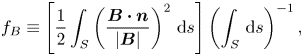 \begin{equation} f_B \equiv \left[ \frac{1}{2} \int_{S} \left( \frac{\boldsymbol{B} \boldsymbol{\cdot} \boldsymbol{n}}{\lvert \boldsymbol{B} \rvert} \right)^{2} \,\textrm{d}s \right] \left( \int_S \,\textrm{d}s \right)^{-1}, \end{equation}
where  $S$ represents the boundary surface and $\boldsymbol {B} \boldsymbol {\cdot } \boldsymbol {n}$ represents the normal field on the boundary. More information on the procedure for generating these coils can be found in Singh et al. (Reference Singh, Kruger, Bader, Zhu, Hudson and Anderston2020).
Table 3. Parameters for the coil set produced for the WISTELL-A configuration using the dimensions in table 2.