


1. INTRODUCTION
In the field of navigation and positioning, technologies based on Radio Frequency (RF) wave propagation are gaining increasing attention. There are various positioning techniques and systems - from global (operating worldwide) to local or personal navigation (operating only inside a particular area, certain place or application). In recent years, the use of local area RF positioning has gained attention, especially in applications where Global Navigation Satellite Systems (GNSS) techniques are not usable (e.g. indoor positioning). RF communication technology is regulated by the IEEE 802.15.4 standard. The use of standardised communication technologies makes positioning much more effective, especially in positioning systems comprised of more than one location device. Since, from a geometric point of view, positioning in RF networks is very often based on trilateration, position accuracy depends on the distance measurement accuracy. There are several different approaches to obtain the distance between nodes in RF technology, including the utilisation of Radio Signal Strength (RSS) (Chen et al., Reference Chen, H. Liu, Yu and Guo2012; Wu et al., Reference Wu, Meng, Lin, He, Peng and Liang2009) to techniques involving Time Of Flight (TOF), Time Of Arrival (TOA), or angle of arrival associated with their communication functionality (Günther and Hoene, Reference Günther, Hoene, Boutaba, Almeroth, Puigjaner, Shen and Black2005; Indelman et al., Reference Indelman, Gurfil, Rivlin and Rotstein2011; Nilson et al., Reference Nilsson, Zachariah, Skog and Händel2013; Obst et al., Reference Obst, Shubert, Mattern, Liberto, Romon and Khoudour2012). Though these techniques show some promising results, the accuracy of such positioning can be improved to allow its use in more demanding applications (Smieja, Reference Smieja2014). Improvement in positioning accuracy can be obtained either by developing new positioning or ranging algorithms, or by new measurement techniques.
A new ranging approach based on the integration of ZigBee communication network protocol and phase shift measurements of RF waves is implemented in the AT86RF233 chip, which provides the possibility to measure distance with much better accuracy than previous techniques. The AT86RF233 is equipped with a Phase Measurement Unit (PMU), which makes it possible to perform ranging using a phase shift measurement as well as perform TOF measurements.
The key advantage of the ZigBee device is its low power consumption. A single device can operate for a very long time (up to several years) on a single battery. It can be used for small mobile devices or embedded into modern cell phones or tablets. A detailed description of ZigBee power consumption can be found in Casilari et al. (Reference Casilari, Cano-García and Campos-Garrido2010).
This paper presents the results of preliminary ranging tests using phase difference measurements based on ZigBee. In this paper, the AT86RF233 chip-ranging results are investigated, and an algorithm to process the measurement results is proposed.
2. DEVICE DESCRIPTION
In the experiment a REB233SMAD-EK device was used. It consists of a pair of network nodes, called “initiator” and “reflector” – as illustrated in Figure 3. Each of the individual nodes consists of a Radio Extender Board (REB) equipped with RF233 AT86RF233 and a Controller Base Board (CBB) equipped with ATxmega256a3 micro-controller (Atmel, 2013). As the user interface a Personal Computer (PC) is used, connected with the initiator node using a Universal Serial Bus (USB) line. The block diagram of the device is presented in Figure 1.

Figure 1. Device block diagram.

Figure 2. Ranging procedure (Atmel, 2013).

Figure 3. Device configuration.
An important feature of an AT86RF233 Transceiver, dedicated primarily for communication in accordance with protocols such as ZigBee, RF4CE, I 6LoWPAN, is the ability to perform ranging, thanks to embedded peripherals such as a Phase Measurement Unit (PMU) or a Time of Flight Module (TOM). In ranging mode, the AT86RF233 chip operates in the 2·4 GHz RF band. The power consumption of the AT86RF233 is approximately 1μA in sleep state and up to 14 mA in active transmit state. Since one of the major disturbances in such measurements is the multipath effect caused by the impact of the environment, to decrease the impact of this effect there is an AS222-92 RF-switch and two pole antennas in the input antenna circuit, as shown in Figure 1. The REB233SMAD-EK device is programmed to perform the ranging procedure and to communicate between the nodes according to the rules based on IEEE802·15·4.
The ranging process between two nodes, preceded by a synchronization phase, is based on the measurement of the RF signal phase shift between the nodes. During one ranging cycle the action is repeated several times for an assumed number of selected frequencies. Every single result is complemented with an additional parameter v that reflects the correctness of the measurement (v = 1 is a valid result and v = 0 is invalid result). The final result of one cycle is expressed as a pair [d; DQF] where d is the calculated and averaged distance and DQF is a Distance Quality Factor (% of valid results in a ranging cycle). The exchange of the frames carrying necessary information such as a request or answer or confirmation, is based on IEEE802·15·4 excluding the actual ranging phase. This is REB233SMAD-EK specific, as depicted in Figure 2.
3. EXPERIMENT
The test measurements were conducted using two nodes placed on known reference baselines, as depicted in Figure 3.
The location of the nodes during each experiment was constant and the reference distances between the nodes were l = 4·86 m, l = 12·76 m, l = 20·00 m, l = 43·80 m, l = 62·00 m. The reference distances were measured with a laser rangefinder. The distance between the antennas mounted on a single node and working in the diversity mode was 12 cm. In further considerations it was assumed to be 0. This assumption is justified because the distance between nodes is from a few metres up to 40–50 metres, while the distance between antennas in a single device is about 10 cm. Therefore, four measured distances are considered as the same distance with an expected accuracy of 10 cm. The vertical location of both nodes was h = 1·50 m above the ground level. Between the nodes there were no obstacles in the Line Of Sight (LOS) or in the close vicinity.
The experiment was performed in two stages. First a series of 300 measurements of distances between nodes 1 and 2 was performed with a 100 ms time interval at each distance. The results from four pairs of antennas (as shown as an example in Figure 4 for 12·76 m) were stored in a file, including distances with corresponding DQF factors.

Figure 4. Raw measurement results.
In the second stage, the results were processed with the algorithm described in Section 4 and were then analysed.
4. EVALUATION OF THE RESULTS AND ALGORITHM FOR DISTANCE DATA PROCESSING
As an example, results of the obtained distance measurements at 12·76 m (which will be called raw measurements in the paper) are depicted in Figure 4. The distance measurement statistics for all measured distances are presented in Table 1. The relative error δ is defined as:
 $$\delta = \displaystyle{{\vert\bar d - {d_0}\vert} \over {{d_0}}}100\% $$
where  $\bar d$ is the average of all samples from one measurement and d 0 is the reference distance.
Table 1. Statistics of the raw distance measurement [cm].

Explicit differences between distances from each pair are caused mainly by a multipath effect, which is typical in such kinds of ranging technology (Liu et al., Reference Hui Liu, Banerjee and Liu2007). In the experiment, the multipath effect is caused by RF waves reflected from the floor. As a result of this phenomenon, fading occurs which causes interference in measurement results. The presence of fading due to interference in LOS causes an unpredictable effect of constructive or destructive interference in RF signal reception that is difficult to eliminate. This disturbance depends strongly on the location of the transmitting and receiving antenna.
The minimum, maximum and standard deviations presented in Table 1 reflect this phenomenon and indicate which pair of antennae is not affected by multipath. The antenna diversity applied in the device allows it to choose the data from the less disturbed pair of antennae, thanks to their slightly different locations.
At each distance the relative error and standard deviations vary depending on the antenna pair. For example at the mean distance of 12·76 m, distances (calculated from all cycles) are in the boundary of 1σ t for pairs 3 and 4, while the values from pairs 1 and 2 differ significantly. This is also confirmed by the histograms in Figures 5 and 6.

Figure 5. Histograms of calculated distance residuals for 12·76 m.

Figure 6. Histograms of DQF for 12·76 m.
Figure 5 shows the histogram of residuals for all antenna pairs. The residuals were calculated using Equation (2).
 $${v_i} = D - {d_i}$$
where v i is the residual, D is the reference distance and d i is the measurement result for one pair of antennae.
At 12·76 m, correct distances (within 1σ t boundary) are present for each pair, although pairs 3 and 4 have the highest number of correct results. This is confirmed by the DQF values (Figure 6). In the case of pairs 3 and 4 there is a much higher number of DQFs with a high value than for pairs 1 and 2.
Another important value for signals is their distribution. As an example, a comparison of the distribution of 12·76 m distance measurements for each pair of antennae with a normal distribution is presented in a normal quartile–quartile plot in Figure 7. Each point on the plot corresponds to one of the quartiles of the distribution of measurement results (y-coordinate) plotted against the same quartile of the normal distribution (x-coordinate). A straight line depicts the normal distribution. The distributions of the measurement results for pairs 3 and 4 are much closer to normal distribution than the distribution of measurement for pairs 1 and 2.

Figure 7. Normal quartile–quartile plots of results from each pair of antennae.
An analysis of Figure 4 shows that in some epochs, the distance closest to the reference distance does not always originate from pair 3 or 4.
Figure 8 depicts the correlation of DQFs and the distances between each pair of antennae. It is a graphical display of a correlation matrix. The size and colour of the circles depicts a correlation between the parameters on the intersection of each row and column. The numbers in the circles are values of correlation translated to percentages. The fact that there is no significant correlation between these variables suggests that the results from each pair can be treated independently.

Figure 8. Plots of correlation between measurement results for antenna pairs.
Preliminary measurement results were processed using simple statistical parameters such as the average of distance and DQF, median of distance and DQF, minimum of distance and DQF, minimum of distance and DQF considering variance, maximum of distance and DQF (for each ranging cycle). The results are summarised in Table 2.
Table 2. Statistics of the filtering results.

The total number of measured distances is 6000 (5 baselines × 4 pairs × 300 measurements). The mean residual calculated from all observations is  $\widehat{{{d_t}}} = 126{\rm \; cm}$, with a standard deviation σ t = 569 cm. The boundary of ${\sigma _t}\; ( \pm \displaystyle{1 \over 2}{\sigma _t} = \pm 284.5\, {\rm cm})$ will be used in the rest of the paper as the maximum error boundary.
Taking into account the lack of correlation it can be assumed that there are four independent data streams (one for each antenna pair). On the basis of the geometry, the most credible data stream is the one with the minimum measured distance value (it is most likely to reflect the direct path between two antennas without multipath effect). The credibility of the data obtained from a single pair of antennas is described by its DQF value.
In order to improve the final ranging results, on the basis of above assumptions, the following algorithm is proposed:
(A) Creating an intermediate data stream of consecutive n cycles
(1) read the data sample from each of the four pairs of antennas (in every ranging cycle)
(2) selection of the smallest value as most credible (without multipath effect)
(3) add the value selected in point (2) to the intermediate stream
Denoting a i, bi, ci, di as values of distance measured in ith cycle for pair 1, 2, 3 and 4 respectively, from the geometric point of view the most credible distance x i is:
(3) $${x_i} = {\rm min}\{ {a_i},{b_i},{c_i},{d_i}\} $$
(B) Smoothing of the intermediate stream from point (A) using a moving average with a structure similar to the finite impulse response filter (FIR) is presented in Figure 9. In Figure 9, the notation z −1 represents a previous sample.


Figure 9. Adaptive moving average/FIR.
According to this algorithm, the final value of distance d is obtained by a sum of the last k elements of an intermediate stream multiplied by the corresponding weights wDQF expressed as:
 $$wDQ{F_i} = \displaystyle{{DQ{F_i} \cdot 100} \over {\mathop \sum \nolimits DQF}}$$
where ∑DQF is a sum of DQF values in one cycle. Multiplication by 100 in the nominator is caused by the DQF values originally expressed as percentages. Additional smoothing effect, especially useful in a dynamic application, is obtained by weighting the last n samples with the arbitrary selected constant weights b 0, b 1, …, b k. The choice of these parameters depends on the scenario in which the device will be used. These parameters provide a smoothing of movement, so they will depend on the system dynamics. In the example presented in this paper these values decrease in arithmetical progression. The algorithm can be presented in the form of Equation (5).
 $${d_n} = \mathop \sum \limits_{k = 0}^{k = N} {x_{(n - k)}}wDQ{F_{(n - k)}}{b_k}$$
The results of applying of the algorithm presented above (with FIR length N = 20) are presented in Figure 10 along with corresponding DQF values and selected pairs of antennas. The number of selections for each pair of antennas is summarised in Table 3. In almost 50% of cycles pair number 3 was selected. This suggests that for antenna pair 3 the distance is measured in a way closest to the LOS.

Figure 10. Minimum distances for each sample.
Table 3. Number of selections for each pair.

The bold line in Figure 10 depicts the results of computations. It is much smoother than the raw measurements. Statistics of the results are provided in Table 4.
Table 4. Statistics of the filtering results [cm].

The results of all of the filtration methods presented above are summarised in Figure 11. Horizontal bars represent the mean residuals for each method at each distance. Black error bars represent standard deviations.
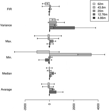
Figure 11. Mean residuals with error bars for each filtering method at different distances.
For each baseline the mean results of proposed filtering method are inside the 1σ boundary. For the presented method the mean residual is increasing with growing distance. In the case of the rest of the methods presented in this paper there is no dependency between distance and mean residual. The smallest residuals, comparable for each filtering method are for the shortest distance. This is because of a short distance – the DQF value is 100% for almost all measurements, so weights are equal and the algorithm is simpler to average.
5. CONCLUSIONS
In this paper, the results of distance measurements performed with AT86RF233 are presented and analysed. The measurement experiment was prepared using an REB233SMADEK device. For the test purposes 6000 data samples were collected. Performed tests confirmed the usability of AT86RF233 in ranging. It provides better ranging accuracy then TOF or RSSI methods.
An algorithm for data processing was proposed based on preliminary statistical evaluation. It consists of a sample selection (forming an intermediate stream) stage and smoothing of the results stage. In the second stage, a weighted moving average is used.
The obtained results show that raw measurements are difficult to interpret and apply in ranging. A simple way to use this data is to apply simple statistical tools such as mean, median or variance (Table 2). A major improvement in ranging results can be obtained using the proposed algorithm. In the case of measurement at 4·86 m distance, the DQF values are saturated so the weighting procedure did not improve the results significantly. The improvement is visible at longer distances where the DQF values varies. For example for the 12·76 m value, using simple statistics gave the best standard deviation of 91 cm while standard deviation after applying the proposed algorithm is 46 cm. The mean residual value also improved from 61 cm (4·78% of total distance) to 11 cm (0·86% of total distance).
The obtained results encourage the use of ranging based on phase shift measurements and the ZigBee protocol in positioning applications. The combination of network communication and ranging in one device allows for further work on collaborative navigation, for example, in indoor applications.


