1. INTRODUCTION
The shortest distance between any two non-antipodal points on a sphere's surface is the only great circle track (GCT) passing through them. The Earth can be considered as a sphere for obtaining the waypoints on the GCT by using great circle sailing (GCS). However, because of the Earth's rotation, the Earth is approximately an oblate spheroid (or ellipsoid of revolution). Consequently, the Mercator chart or an Electronic Chart Display and Information System (ECDIS) usually uses the WGS 84 (World Geodetic System ellipsoid of 1984). A great circle other than a meridian or the equator is a curved line whose true direction changes continually, thus navigators do not usually attempt to follow it exactly. Instead, they select a number of waypoints along the GCT, construct rhumb lines between the waypoints on the Mercator chart or in the ECDIS, and then steer along these rhumb lines (Bowditch, Reference Bowditch2002). In practical navigation, the waypoints on the GCT are entered into the ECDIS, GPS, or a fully integrated navigation system. Then, the vessel is programmed to follow the GCT by sailing from waypoint to waypoint by rhumb line, with allowances made for wind and current effects.
When the Earth is regarded as a sphere, the navigator has to give initial conditions for obtaining the waypoints along the GCT. Generally speaking, these given initial conditions include: giving the longitudes of the waypoints to obtain their latitudes (Condition 1); giving the great circle distances to yield the latitudes and longitudes of the waypoints (Condition 2). Once all the waypoints on the GCT are available, the navigator needs to take the Earth as an oblate spheroid for practical navigation. Because the GCT is composed of legs of rhumb lines, the course and distance of the rhumb line between two adjacent waypoints can be determined by using the Mercator sailing.
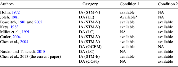
The spherical triangle method (STM) with a reference point at the vertex (called STM-V) has been developed to solve the waypoints on the GCT for many years. It can handle the waypoints problem under Conditions 1 or 2 (Holm, Reference Holm1972; Bowditch, Reference Bowditch1981, Reference Bowditch2002; Keys, Reference Keys1983; Cutler, Reference Cutler2004; Chen et al., Reference Chen, Hsu and Chang2004). The advantage of this method is that the solved formulae are simplified because the method uses Napier's rules of right-angled spherical triangles. Finding the equator crossing point of the GCT is easier than finding the vertex of the GCT. In addition, when the supplemental theorem is introduced, the right-angled spherical triangles can be converted into quadrantal spherical triangles (Clough-Smith, Reference Clough-Smith1966). Therefore, a method with the reference point at the equator crossing point (called STM-E) should be available. The STM-E has the same advantage as the STM-V and can also deal with the waypoints problem under Condition 1 or 2. However, a common disadvantage of the STM-V and STM-E is that the reference point should be determined in advance. Owing to this disadvantage, both methods are usually considered as a type of indirect approach (IA).
To overcome this shortcoming, some researchers take the departure point as the reference point. This means one can replace the Greenwich meridian by the meridian of the departure point and this is usually called the relative longitude concept. Similarly, Jofeh (Reference Jofeh1981) constructed a linear equation (LE) of the GCT, which appears as a straight line on the polar gnomonic chart. According to his method, the latitudes of the waypoints are determined only under Condition 1. Unfortunately, when the departure and destination points are located in different hemispheres, the method fails. Later, Miller et al. (Reference Miller, Moskowitz and Simmen1991) first used the technique of the fixed coordinates system to construct a vector expression of the waypoints and then adopted linear combination (LC) of a vector basis to formulate another vector expression. Comparing the components of the different vector expressions yields three key formulae, that is, five-parts formula (x-component), five-parts formula (y-component) and side cosine law (z-component). Then, a combination of the five-parts formula (x-component) and the side cosine law (z-component) can handle the waypoints problem but only under Condition 2. Thereafter, Chen et al. (Reference Chen, Hsu and Chang2004) first combined the technique of the fixed coordinates system with the relative longitude concept (FCRL) and then proposed the great circle equation method (GCEM), in which the great circle equation is formulated by vector algebra. It is found that the GCEM can deal with the waypoints problem only under Condition 1. In addition, like Miller et al. (Reference Miller, Moskowitz and Simmen1991), Nastro and Tancredi (Reference Nastro and Tancredi2010) adopted linear combination (LC) of a different vector basis with the FCRL, also reaching three key formulae. That is, five-parts formula (x-component), sine law (y-component) and side cosine law (z-component). Then, the sine law divided by the five-parts formula obtains the four-parts formula. A combination of this formula and the yielded side cosine law can handle the waypoints problem but only under Condition 2. However, tedious derivations make their solutions hard to understand. In contrast to the IA, the methods mentioned above all belong to a type of direct approach (DA). The comparison of the mentioned methods is listed in Table 1. In this table, it is found that the DA can solve the waypoints problem under either Condition 1 or Condition 2; while the IA can deal with the problems under both Conditions 1 and 2.
Table 1. A comparison of different methods for solving the GCS.

* This method fails when departure and destination points are located in different hemispheres.
To overcome the complex derivations (Miller et al., Reference Miller, Moskowitz and Simmen1991; Nastro and Tancredi, Reference Nastro and Tancredi2010), the concise derivation of the formulae by using multiple products of vector algebra (VA-MP) with the FCRL is proposed to solve the waypoints problem under Condition 2. Once the initial great circle course is fixed (COFI), the GCT can be determined. With this characteristic, the proposed approach is named the “COFI method”. Further, to tackle the waypoints problem covering Conditions 1 and 2, a program, based on the COFI method and the simplified GCEM, has been developed for the practical navigator. In addition, because the STM-E can deal with the waypoints problem under two given conditions, derivations of the method are also included in this article.
Theoretical backgrounds of the STM-E, the COFI method and the simplified GCEM are presented in Section 2. Section 3 describes the computation procedures of the COFI method and the simplified GCEM. Validated examples are given in Section 4. Finally, the work is summarised and concluded in Section 5.
2. THEORETICAL BACKGROUNDS
2.1. Deriving Formulae for the STM-E
As mentioned in the previous section, the supplemental theorem can be used to derive the formulae of the STM-E for solving the waypoints problem. The supplemental theorem describes (Clough-Smith, Reference Clough-Smith1966):
“The angles in the polar triangle are supplements of the corresponding sides in the primitive triangle, and the sides in the polar triangle are supplements of the corresponding angles in the primitive triangle.”
Due to this property, those formulae used in right-angled spherical triangles can also work in quadrantal spherical triangles. In addition, because the great circle arc from the equator crossing point to the pole should be 90°, the equator crossing point, the pole nearer the departure and waypoints along the GCT can form numerous quadrantal spherical triangles as shown in Figure 1. Consequently, the solving steps of the STM-E are presented as follows. All the symbols used below are listed in the Appendix.
Figure 1. An illustration of the STM-E for solving the problem of GCS.
Step 1. Finding the great circle distance (D) and the initial great circle course angle (C) as shown in Figure 1. The great circle distance and the initial course angle can be calculated by the side cosine law and the four-parts formula of the spherical trigonometry, respectively as (Chen et al., Reference Chen, Hsu and Chang2004):
 $$\cos D = \sin L_{\rm F} \sin L_{\rm T} + \cos L_{\rm F} \cos L_{\rm T} \cos DLo,$$
 $$\tan C = \displaystyle{{\sin DLo} \over {(\cos L_{\rm F} \tan L_{\rm T} ) - (\sin L_{\rm F} \cos DLo)}}.$$
Step 2. Finding the longitude of the equator crossing point, λ E, as shown in Figure 2. By using Napier's rules of quadrantal spherical triangles, the following two formulae can be yielded as:
 $$\tan DLo_{{\rm FE}} = - \sin L_{\rm F} \tan C,$$
 $$\sin C_{\rm E} = \cos L_{\rm F} \sin C.$$
Figure 2. An illustration of finding the equator crossing point on the GCT by using Napier's rule of quadrantal spherical triangles.
Note that if DLo FE has the same name as DLo (i.e. both West or both East) and λ F is available, λ E can be obtained by Equation (3). In addition, C E, can be obtained by Equation (4) and it will be used in the following step.
Step 3. Finding the latitudes and longitudes of the waypoints along the GCT is shown in Figure 3. Since only C E is available, the given condition is necessary for obtaining the waypoints. By using Napier's rules of quadrantal spherical triangles, we can yield the following formulae under both Conditions 1 and 2.
Figure 3. An illustration of finding the waypoints on the GCT by using Napier's rule of quadrantal spherical triangles.
Condition 1. When λ X is given, DLo EX can be obtained. Then, L X can be calculated from the following formula
 $$\tan L_X = \pm \cot C_{\rm E} \sin DLo_{{\rm E}X}. $$
Note that if DLo EX is the contrary name to DLo (i.e. one East and one West), the right-hand side of Equation (5) should take the positive sign. It means L X and L F are located in the same hemisphere. Conversely, if DLo EX has the same name as DLo, the right-hand side of Equation (5) should be treated as negative sign. It means L X and L F are located in different hemispheres.
Condition 2. When the D EX is given, the waypoints can be obtained from the formulae,
 $$\sin L_X = \cos C_{\rm E} \sin D_{{\rm E}X}, $$
 $$\tan DLo_{{\rm E}X} = \sin C_{\rm E} \tan D_{{\rm E}X}. $$
In Equation (6), note that when L X is smaller than L F, the waypoints are on the GCT. This means L X and L F are located in the same hemisphere. Thus, L X is taken as the positive. Similarly, when L X is smaller than L T, the waypoints are on the GCT but L X and L T are located in different hemispheres. In this regard, L X is taken as the negative. In Equation (7), if the value of tan DLo EX is negative, (180°−DLo EX) should replace (−DLo EX) for satisfying the definition of DLo EX. As for the designated east or west of DLo EX, it depends on the sign of L X. If L X is positive, DLo EX is contrary name to DLo. However, if L X is negative, DLo EX has the same name as DLo. Obviously, too many judgments of sign conventions arise in the solving procedures of the STM-E and this makes use of this method hard work for the navigator. However, the STM-E method still offers a way to solve the waypoints problem.
2.2. Deriving Formulae for the COFI method
As the Earth is treated as a unitary sphere, the vector expression of any point G(L, λ) on the Earth's surface in a Cartesian coordinates system can be written as:
 $${\bf {\mathop{G}\limits^{\rightharpoonup}} }= \left[ {\cos L\cos \lambda, \;\cos L\sin \lambda, \;\sin L} \right],\;L = \left[ { - \displaystyle{\pi \over 2},\;\displaystyle{\pi \over 2}} \right],\;\lambda = [0,{\rm 2}\pi {\rm )}{\rm.} $$
To avoid an additional judgment of sign convention, the technique of the fixed coordinates system is first considered, that is, the north latitude is treated as a positive value and the south latitude is taken as a negative one. As shown in Figure 4, introducing the relative longitude concept, the unit vectors of the North Pole (P), the departure (F), the destination (T) and the waypoints (X) on a GCT can be expressed as:
 $${\bf {\mathop{P}\limits^{\rightharpoonup}} } = \left[ {0,{\rm} 0,{\rm} 1} \right],$$
 $${\bf {\mathop{F}\limits^{\rightharpoonup}} } = \left[ {\cos L_{\rm F}, {\rm} 0,{\rm} \sin L_{\rm F}} \right],$$
 $${\bf {\mathop{T}\limits^{\rightharpoonup}} } = \left[ {\cos L_{\rm T} \cos DLo,\,\cos L_{\rm T} \sin DLo,\;\sin L_{\rm T}} \right],$$
 $${\bf {\mathop{X}\limits^{\rightharpoonup}} } = \left[ {\cos L_X \cos DLo_{{\rm F}X}, \,\cos L_X \sin DLo_{{\rm F}X}, \;\sin L_X} \right].$$
Figure 4. An illustration of four position vectors.
When the vector algebra is introduced, derivations of the formulae used for the COFI will be simpler and clearer than those of the DA. Therefore, we adopt multiple products of the vector algebra to yield the great circle distance, the initial course and the waypoints on the GCT (Spiegel, Reference Spiegel, Lipschutz and Spellman2009; Chen et al., Reference Chen, Hsu and Chang2004).
2.2.1. Obtaining the great circle distance
As shown in Figure 4, there are two ways to obtain the great circle distance. One is to yield the great circle arc (D) of the spherical triangle by the dot product of two unit vectors. That is,
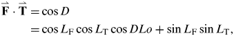 $$\eqalign{{\bf {\mathop{F}\limits^{\rightharpoonup}} } \cdot {\bf {\mathop{T}\limits^{\rightharpoonup}} } = & \cos D \cr {\rm =} & \cos L_{\rm F} \cos L_{\rm T} \cos DLo + \sin L_{\rm F} \sin L_{\rm T},} $$
in which the first row of the above equation uses the geometric definition of vector product, while the second row uses the algebraic operation of vector product.
Another method is to adopt the dot product of two normal vectors,  $({\bf {\mathop{P}\limits^{\rightharpoonup}} } {\bf \times} {\bf {\mathop{T}\limits^{\rightharpoonup}} } )$ and $({\bf {\mathop{P}\limits^{\rightharpoonup}} } {\bf \times} {\bf {\mathop{F}\limits^{\rightharpoonup}} } )$, to yield the dihedral angle (DLo) of the spherical triangle. Therefore,
 $$\eqalign{( {\bf {\mathop{P}\limits^{\rightharpoonup}} }\times {\bf {\mathop{T}\limits^{\rightharpoonup}} }) \cdot ({\bf {\mathop{P}\limits^{\rightharpoonup}} } \times {\bf {\mathop{F}\limits^{\rightharpoonup}} }) = & \cos L_{\rm T} \cos L_{\rm F} \cos DLo \cr {\rm =} & \left| {\matrix{ {{\rm (}{\bf {\mathop{P}\limits^{\rightharpoonup}} } \cdot {\bf {\mathop{P}\limits^{\rightharpoonup}} }{\rm )}} & {{\rm (}{\bf {\mathop{P}\limits^{\rightharpoonup}} } \cdot {\bf {\mathop{F}\limits^{\rightharpoonup}} }{\rm )}} \cr {{\rm (}{\bf {\mathop{T}\limits^{\rightharpoonup}} } \cdot {\bf {\mathop{P}\limits^{\rightharpoonup}} }{\rm )}} & {{\rm (}{\bf {\mathop{T}\limits^{\rightharpoonup}} } \cdot {\bf {\mathop{F}\limits^{\rightharpoonup}} }{\rm )}} \cr}} \right| = \cos D - \sin L_{\rm F} \sin L_{\rm T}.} $$
Similarly, two rows of Equation (14) represent the same mathematical meanings as those of Equation (13). After arranging Equations (13) or (14), we can write the same governing equation as:
 $$\cos D = \sin L_{\rm F} \sin L_{\rm T} + \cos L_{\rm F} \cos L_{\rm T} \cos DLo.$$
Equation (15) is the well-known side cosine law of spherical trigonometry.
2.2.2. Obtaining the initial great circle course angle
To yield the initial great circle course angle, that is, the dihedral angle (C) of the spherical triangle, we adopt the dot product of two normal vectors,  $({\bf {\mathop{F}\limits^{\rightharpoonup}} } {\bf \times} {\bf {\mathop{P}\limits^{\rightharpoonup}} } )$ and $({\bf {\mathop{F}\limits^{\rightharpoonup}} }\! \times\! {\bf {\mathop{T}\limits^{\rightharpoonup}} } )$. Hence,
 $$\eqalign{({\bf {\mathop{F}\limits^{\rightharpoonup}} } {\bf \times} {\bf {\mathop{P}\limits^{\rightharpoonup}} } ) \cdot ({\bf {\mathop{F}\limits^{\rightharpoonup}} } {\bf \times} {\bf {\mathop{T}\limits^{\rightharpoonup}} } ) = & \cos L_{\rm F} \sin D\cos C \cr {\rm =} & \sin L_{\rm T} - \sin L_{\rm F} \cos D,} $$
in which the first row uses the geometric definition of vector products, while the second row uses the algebraic operation of vector products. Rearranging Equation (16) obtains the governing equation as:
 $$\cos C = \displaystyle{{\sin L_{\rm T} - \sin L_{\rm F} \cos D} \over {\cos L_{\rm F} \sin D}}.$$
Equation (17) is another form of the side cosine law of the spherical trigonometry.
2.2.3. Obtaining the latitudes of waypoints along the GCT
As the initial great circle course is fixed, the GCT can be determined. Then, giving the great circle distance from the departure point (Condition 2) we can obtain every waypoint along the GCT. Replacing the parameter vector  ${\bf {\mathop{T}\limits^{\rightharpoonup}} }$ of Equation (16) by the variable vector ${\bf {\mathop{X}\limits^{\rightharpoonup}} }$ yields
 $$\eqalign{({\bf {\mathop{F}\limits^{\rightharpoonup}} } \times {\bf {\mathop{P}\limits^{\rightharpoonup}} } ) \cdot ({\bf {\mathop{F}\limits^{\rightharpoonup}} } \times {\bf {\mathop{X}\limits^{\rightharpoonup}} } ) = & \cos L_{\rm F} \sin D_{{\rm F}X} \cos C \cr = & \sin L_X - \sin L_{\rm F} \cos D_{{\rm F}X}.} $
Rearranging Equation (18) obtains
 $$\sin L_X = \sin L_{\rm F} \cos D_{{\rm F}X} + \cos L_{\rm F} \sin D_{{\rm F}X} \cos C.$$
The above equation is also the side cosine law of the spherical trigonometry.
2.2.4. Obtaining the longitudes of waypoints along the GCT
Replacing parameter vector ${\bf {\mathop{T}\limits^{\rightharpoonup}} }$ of Equation (14) by variable ${\bf {\mathop{X}\limits^{\rightharpoonup}} }$ vector yields
 $$\eqalign{({\bf {\mathop{P}\limits^{\rightharpoonup}} } \times{\bf {\mathop{X}\limits^{\rightharpoonup}} } ) \cdot ({\bf {\mathop{P}\limits^{\rightharpoonup}} } \times {\bf {\mathop{F}\limits^{\rightharpoonup}} } ) = & \cos L_X \cos L_{\rm F} \cos DLo_{{\rm F}X} \cr = & \cos D_{{\rm F}X} - \sin L_{\rm F} \sin L_X.} $$
Rearranging Equation (20), we have
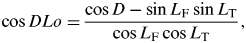
 $$\cos DLo_{{\rm F}X} = \displaystyle{{\cos D_{{\rm F}X} - \sin L_{\rm F} \sin L_X} \over {\cos L_{\rm F} \cos L_X}}. $$
The above equation is another form of the side cosine law of spherical trigonometry.
Note that Equations (19) and (21) are a set of the governing equations to obtain the latitudes and longitudes of the waypoints along the GCT under Condition 2. In summary, formulae used in the COFI method are only a form of the side cosine law of spherical trigonometry. Therefore, introducing the vector algebra into derivations of the COFI method makes this method simpler and clearer than the conventional approaches.
2.3. Reformulating the formulae used for the GCEM
To solve the waypoints problem covering Conditions 1 and 2, the GCEM and the COFI method should be combined for the practical navigator. Therefore, revisiting and simplifying the formulae of the GCEM are described as follows.
2.3.1. Revisiting the GCEM
Those formulae used for the GCEM are briefly revisited here (Chen et al., Reference Chen, Hsu and Chang2004). As shown in Figure 4, if three vectors are coplanar, the scalar triple product is equal to zero. That is,
 $$({\bf {\mathop{F}\limits^{\rightharpoonup}} } \times{\bf {\mathop{T}\limits^{\rightharpoonup}} } ) \cdot {\bf {\mathop{X}\limits^{\rightharpoonup}} } = 0.$$
Now, assuming
 $${\bf {\mathop{F}\limits^{\rightharpoonup}} } {\bf \times} {\bf {\mathop{T}\limits^{\rightharpoonup}} }= \left[ {a,{\rm} b,{\rm} c} \right],$$
and substituting Equations (10) and (11) into Equation (23) yield
 $$a = - \sin L_{{\rm F}} \cos L_{{\rm T}} \sin DLo,$$
 $$b = \sin L_{\rm F} \cos L_{\rm T} \cos DLo - \cos L_{\rm F} \sin L_{\rm T}, $$
 $$c = \cos L_{\rm F} \cos L_{\rm T} \sin DLo.$$
Finally, the Great Circle Equation can be formulated as
 $$a\cos L_X \cos DLo_{{\rm F}X} + b\cos L_X \sin DLo_{{\rm F}X} + c\sin L_X = 0.$$
Note that Equation (27) implies the information of the great circle, for example, the waypoints along the GCT, the equator crossing point and the vertex.
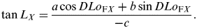
1. The waypoints along the GCT: When λ X is given, DLo FX can be obtained. Rearranging Equation (27) yields
(28) $$\tan L_X = \displaystyle{{a\cos DLo_{{\rm F}X} + b\sin DLo_{{\rm F}X}} \over { - c}}.$$
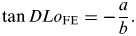
2. The equator crossing point: Since L E=0, substituting it into Equation (28) yields
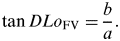
(29)$$\tan DLo_{{\rm FE}} = - \displaystyle{a \over b}.$$3. The vertex: When the vertex is the highest latitude for the great circle, the first derivative of Equation (28) must be zero. Therefore, we have
(30)$$\tan DLo_{{\rm FV}} = \displaystyle{b \over a}.$$
Substituting the above result into Equation (28) yields
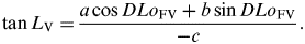 $$\tan L_{\rm V} = \displaystyle{{a\cos DLo_{{\rm FV}} + b\sin DLo_{{\rm FV}}} \over { - c}}.$$
2.3.2. Simplifying formulae used for the GCEM
Because Equation (25) used for obtaining the parameter, b, is complex, we need to simplify it for a practical use. First, Equations (15) and (17) can be rewritten as
 $$\cos DLo = \displaystyle{{\cos D - \sin L_{\rm F} \sin L_{\rm T}} \over {\cos L_{\rm F} \cos L_{\rm T}}}, $$
 $$\sin L_{\rm T} = \sin L_{\rm F} \cos D + \cos L_{\rm F} \sin D\cos C.$$
Then, substituting Equations (32) and (33) into Equation (25) and rearranging it yield
 $$b = - \sin D\cos C.$$
Introducing the sine law of spherical trigonometry, that is,
 $$\cos L_{\rm T} \sin DLo = \sin D\sin C,$$
and substituting Equation (35) into Equations (24) and (26), respectively yield
 $$a = - \sin L_{{\rm F}} \sin D\sin C,$$
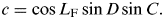 $$c = \cos L_{\rm F} \sin D\sin C.$$
Therefore, the concise formulae used for the simplified GCEM are as follows.
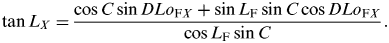
1. The waypoints along the GCT: Substituting Equations (34), (36) and (37) into Equation (28) and rearranging it yield
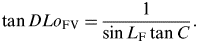
(38)$$\tan L_X = \displaystyle{{\cos C\sin DLo_{{\rm F}X} + \sin L_{\rm F} \sin C\cos DLo_{{\rm F}X}} \over {\cos L_{\rm F} \sin C}}.$$2. The equator crossing point: Substituting Equations (34) and (36) into Equation (29) yields
(39)$$\tan DLo_{{\rm FE}} = - \sin L_{\rm F} \tan C.$$3. The vertex: Substituting Equations (34) and (36) into Equation (30) yields
(40)$$\tan DLo_{{\rm FV}} = \displaystyle{1 \over {\sin L_{\rm F} \tan C}}.$$

Further, substituting Equations (34), (36) and (37) into Equation (31) yields
 $$\tan L_V = \displaystyle{{\cos C\sin DLo_{{\rm F}V} + \sin L_{\rm F} \sin C\cos DLo_{{\rm F}V}} \over {\cos L_{\rm F} \sin C}}.$$
3. COMPUTATION PROCEDURES AND NUMERICAL PROGRAM
The great circle sailing problem is first to obtain the waypoints along the GCT. Then, the course and distance of the rhumb line between two adjacent waypoints can be determined by using the Mercator sailing. All required formulae used for the numerical program are listed as
 $$M = a_e \ln \left[ {\tan \left( {45{\curr { \char "000B0}}} + \displaystyle{L \over 2}} \right) \times \left( {\displaystyle{{1 - e\sin L} \over {1 + e\sin L}}} \right)^{\textstyle{e \over 2}}} \right],$$
in which e=0·081819190842622 for WGS 84 (NIMA, 2000) and a e=3437·74677078 nautical miles (nm) (Bowditch, Reference Bowditch2002).
According to the formulae of the Mercator sailing,
 $$\ell = L_{{\rm X}_{i + 1}} - L_{{\rm X}_i}, \;dlo = \lambda _{{\rm X}_{i + 1}} - \lambda _{{\rm X}_i}, \;m = M_{{\rm X}_{i + 1}} - M_{{\rm X}_i}, $$
 $$\tan cm = \displaystyle{{dlo \times 60\prime} \over m},$$
 $$dm = \left\{ {\matrix{ {\ell \sec {\kern 1pt} cm} , & & {cm \ne 90{\curr { \char "000B0}}} \cr {dlo\cos {\kern 1pt} L_{{\rm X}_i}}, & & {cm = 90{\curr { \char "000B0}}} \cr}} \right.$$
3.1. Computation procedures for the simplified GCEM and the COFI method
3.2. Developing the numerical program
A GCS program, called “GCSPro”, covering Conditions 1 and 2, has been developed based on the COFI method and the simplified GCEM. For ease of use, GCSPro uses Visual Basic (VB) with a graphical user interface (GUI) for programming. In addition, for the purpose of choosing reasonable numbers of the waypoints, a diagram of total Mercator distance versus waypoints number (called tMd-n diagram) is provided for the navigator.
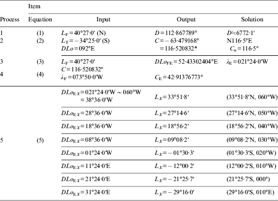
Table 2. Results of solving waypoints along the GCT under λ X by using the STM-E in Example 1.
* Since tan(−θ)=tan(180°−θ), (−θ) is replaced as (180°−θ).
4. DEMONSTRATED EXAMPLES AND DISCUSSION
4.1. Example 1
A vessel is proceeding from New York (USA) to Cape Town (South Africa). The master desires to use the great circle sailing from L40°27·0′N, λ073°50·0′W to L34°25·0′S, λ018°10·0′E.
4.1.1. Required
Calculate the following cases under different given conditions by using the STM-E.
1. Calculate the great circle distance, initial course and the latitudes and longitudes of the waypoints along the GCT at longitude 060°W and at each 10° of longitude thereafter to longitude 010°E (Condition 1).
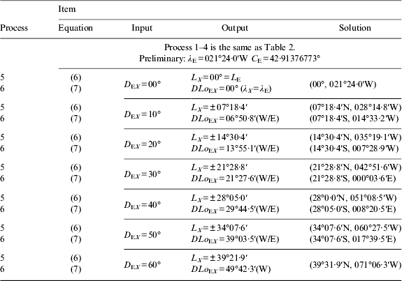
2. Calculate the latitudes and longitudes of the waypoints along the GCT at equal interval of great circle distance, 600 (10°) nautical miles (nm), from the equator crossing point (Condition 2).
4.1.2. Solution
1. The STM-E is adopted to solve the waypoints along the GCT under Condition 1. Results and the solving procedures with the suggested formulae are shown in Table 2.
2. The STM-E is adopted to solve the waypoints along the GCT under Condition 2. Results and the solving procedures with the suggested formulae are shown in Table 3.
Table 3. Results of solving waypoints along the GCT under D EX by using the STM-E in Example 1.
4.1.3. Discussion
In this example, although the STM-E can solve waypoints problems under Conditions 1 and 2, many sign convention judgments arise in the solving procedure of the STM-E. Anyway, it still offers another solving approach for the IA.
4.2. Example 2
A vessel is proceeding from San Francisco (USA) to Sydney (Australia). The navigator desires to use great circle sailing from L37°47·5′N, λ122°27·8′W to L33°51·7′S, λ151°12·7′E (Bowditch, Reference Bowditch1981, P.616–618).
4.2.1. Required
Using GCSPro to calculate the latitudes and longitudes of the waypoints on the GCT 360 nm apart (Condition 2), and the information for the great circle (eg. the great circle distance, initial course, the equator crossing point and the vertices).
4.2.2. Solution
GCSPro is used to solve the waypoints on the GCT under Condition 2. Results including of the waypoints, great circle information, and a tMd-n diagram are shown in Figure 5. The comparison of results obtained by the COFI method and those by the Ageton method (tabular method) is shown in Table 4. In addition, when the “show data” button in Figure 5 is clicked, detailed numerical information of total Mercator distance versus numbers of waypoints will display in the format shown in Table 5.
Figure 5. Results of running the GCSPro under Condition 2 in Example 2.
Table 4. A comparison of results obtained by the Ageton method and the COFI method in Example 2.

* Resource: Bowditch, Reference Bowditch1981, P.616–618.
Table 5. The relationship between total Mercator distance (nm) and waypoint number on the GCT in Example 2.

4.2.3. Discussion
In this example, the COFI method has been validated successfully. In Table 4, it is found that the COFI method is more accurate than the Ageton method because the former is free of rounding errors, which was also reported in Bowditch (Reference Bowditch2002). As for Table 5, the total Mercator distance of 16 waypoints is nearly equal to that of 8 waypoints and their distance difference is less than 1 nm. An optimum number of waypoints can be determined from this table for the navigator.
4.3. Example 3
A vessel is proceeding from Sydney (Australia) to Balboa (Panama). The master desires to use the great circle sailing from L33°51·5′S, λ151°13·0′E, to L08°53·0′N, λ079°31·0′W (Chen et al, Reference Chen, Hsu and Chang2004. pp. 317–319).
4.3.1. Required
Using GCSPro to calculate the latitudes and longitudes of the waypoints on the GCT at longitude and at each 10 degrees of longitude thereafter to longitude (Condition 1), and the information for the great circle (eg. the great circle distance, initial course, the equator crossing point and the vertices).
4.3.2. Solution
GCSPro is used to solve the waypoints along the GCT under Condition 1 successfully. Results including the waypoints, great circle information and a tMd-n diagram are shown in Figure 6.
Figure 6. Results of running the GCSPro under Condition 1 in Example 3.
4.3.3. Discussion
Based on the proposed COFI method and the simplified GCEM, the developed GCSPro program has been validated by Examples 2 and 3. It is found that the GCSPro program shows the advantages of completeness and practical application.
5. CONCLUSIONS
In this paper, the COFI method has been developed to calculate the waypoints along the GCT successfully using the multiple products of the vector algebra (VA-MP). Due to fixing the initial great circle course, the GCT can be determined and the waypoints along the GCT can be calculated directly. In addition, without tedious derivations, the COFI method is simpler and more straightforward than the conventional methods. A program, GCSPro, for calculating GCT problems has been validated by the practical examples. It is found that the program can be user friendly and effectively operated by the navigator under two given initial conditions. Finally, the STM-E has been derived and also offers another way to solve the waypoints problem successfully.
ACKNOWLEDGEMENT
Constructive suggestions by Dr. Jiang-Ren Chang are highly appreciated. In addition, financial support from the National Science Council, Taiwan under contract number: NSC 95-2221-E-019-092- and NSC 96-2628-E-019-022-MY3 are acknowledged.
APPENDIX