


1. INTRODUCTION
In classical celestial navigation a running fix is obtained by combining sights taken at two different times and positions. The relative distance and bearing of the two positions are assumed to be known from the ship's course and speed.
In practice such a fix is often obtained graphically by plotting Lines of Position (LoP) LoP1 and LoP2 associated with the first and second sights respectively on a nautical chart or plotting sheet. LoP1 is then translated or advanced by a distance and direction that reflects the rhumb line track of the vessel between the two observations. The point where the advanced LoP1 crosses LoP2 provides the running fix. This procedure generally works satisfactorily on small scales over which the Earth's surface can be represented by a plane and LoPs are well approximated by straight lines.
On the surface of a sphere an LoP obtained from a celestial sight becomes a Circle of Position (CoP) centred on the point on the Earth's surface where the observed celestial body is directly overhead. This is referred to as the body's Geographic Position (GP).
Attempts have been made to extend the notion of advancing an LoP to the case of the sphere with the idea that the running fix could then be found as the intersection point of two circles using double altitude or similar methods (Metcalf Reference Metcalf1991; Zevering Reference Zevering2006). The problem, as has been pointed out previously (Williams Reference Williams1998; Huxtable, Reference Huxtable2006), is that if each point on a CoP is individually advanced on a rhumb line course of specified distance and bearing, the resultant locus of points is no longer a circle. This point is illustrated in Figure 1. It follows that any approach that purports to obtain a running fix on the surface of a sphere as the intersection of two circles is fundamentally flawed.

Figure 1. Effect of advancing each point on an initial Circle of Position indicated by the heavy curve by 2000 nm (dashed curve) and 4000 nm (dotted curve) on a course of 160° True. The centre of the original CoP is shown. Large displacements have been chosen to make the resulting distortions clearly visible.
An equation satisfied by points on the advanced CoP and its generalization to the ellipsoid has been given by Williams (Reference Williams1998) who suggests solving a pair of non-linear simultaneous equations to obtain the fix.
On reflection it is perhaps unfortunate that the graphical technique used on a plane for obtaining a running fix has so strongly coloured the thinking and influenced the approaches when it comes to a running fix on curved surfaces where advancing or transferring an LoP offers no obvious advantages.
In this note the problem of the running fix on the surface of the Earth is approached in a manner that avoids the need for advancing an LoP as a whole. Indeed the method will be described for the case of an ellipsoidal Earth as it is only marginally more complicated than the spherical case.
It is to be expected that, because of the complex mixture of logarithms and trigonometric functions that appear in Mercator sailing formulae, solutions will necessarily be numerical in nature even in the case of a sphere. It will be shown that the numerical problem can be reduced to one of finding the root of a function of just one variable and does not require solving simultaneous non-linear equations.
On an ellipsoid a celestial sight yields a set of possible positions that lie neither on a circle nor a line. In what follows LoP should considered to stand for Locus of Position.
2. RUNNING FIX ON THE SURFACE OF AN ELLIPSOID
Assume a sight of a celestial body is made when the ship is initially at a position denoted P 1. The sight yields the zenithal distance, ZD1, for the observed body. At the instant of observation the GP of the body is specified by its declination, δ1, and Greenwich Hour Angle, GHA1. From this information it can be determined that P 1 lies somewhere on a locus of position LoP1. The vessel then travels a distance, D, on a rhumb line course of bearing, C, measured east from north to a position denoted P 2 where a second sight is made. This sight produces a corresponding set of parameters ZD2, δ2 and GHA2 which determines that the vessel's position, denoted P 2, lies somewhere on LoP2.
The general running fix requires finding positions P 1 and P 2 that satisfy the following conditions
-
1) P 1 lies on LoP1
-
2) P 2 lies a distance D from P 1 along a rhumb line course with bearing C.
-
3) P 2 lies on LoP2
The required fix is given by P 2. In general it is to be expected that two geographically widely separated sets of points can be found to satisfy these conditions. A similar situation arises in double altitude sights. A reasonable initial estimate of position ensures that the correct solution is selected.
Assume a value L 1 for the latitude of position P 1 and find the corresponding longitude, λ1, such that P 1 lies on LoP1 using the equation
 $$\lambda_1 =-\hbox{GHA}_1 \pm \cos^{-1}\left({\displaystyle{{\cos ZD_1 -\sin \delta_1 \sin L_1}\over{\cos \delta_1 \cos L_1}}}\right)$$
The upper (lower) sign applies when the object lies to the observer's west (east). This formula follows from the familiar cosine rule of spherical trigonometry but because geodetic or astronomical latitude and longitude on the surface of an ellipsoid are defined from the direction of the normal to the surface it applies to both the sphere and ellipsoid. An explicit proof is given by Williams (Reference Williams1998, Section 9.3). On the sphere, points on the LoP all lie the same geodesic distance from the GP; however this is not true for an ellipsoid.
Compute the position P 2, with latitude L 2 and longitude, λ2, located a distance D along a rhumb line course of bearing C from P 1. This is the direct Mercator sailing problem which can be solved, in principle, using the equations
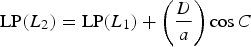 $$\hbox{LP}\lpar {L_2}\rpar =\hbox{LP}\lpar {L_1} \rpar +\left({\displaystyle{{D}\over{a}}} \right)\cos C $$
 $$\lambda_2 = \lambda_1 +\lpar {\hbox{MP}\lpar {L_2}\rpar -\hbox{MP}\lpar {L_1}\rpar }\rpar \tan C $$
Here a is the Earth's equatorial radius and MP(ϕ) is the meridional part:
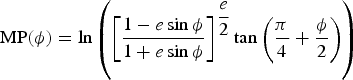 $$\hbox{MP}\lpar \phi \rpar =\ln \left({\left[{\displaystyle{{1-e\sin \phi}\over{1+e\sin \phi}}}\right]^{\displaystyle{{e}\over{2}}}\tan \left({\displaystyle{{\pi}\over{4}}+\displaystyle{{\phi}\over{2}}}\right)}\right)$$
When L 2 = L 1 Equation (2) becomes
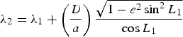 $$\lambda_2 = \lambda_1 +\left({\displaystyle{{D}\over{a}}}\right)\displaystyle{{\sqrt {1-e^2\sin ^2L_1}}\over{\cos L_1}}$$
The function LP(ϕ) is the meridional arc length in units of a from the equator to the latitude ϕ:
 $$LP\lpar \phi \rpar =\lpar {1-e^2} \rpar \int\limits_0^\phi {\lpar {1-e^2\sin^2\theta} \rpar ^{-\displaystyle{{3}\over{2}}}d\theta}$$
This can be written in terms of Legendre elliptic integrals of the second or third kind:
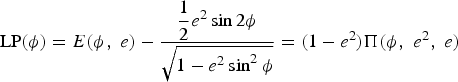 $$\hbox{LP}\lpar \phi \rpar =E\lpar {\phi\comma \; e} \rpar -\displaystyle{{\displaystyle{{1}\over{2}} e^2\sin 2\phi}\over{\sqrt {1-e^2\sin ^2\phi}}}=\lpar {1-e^2} \rpar \Pi \lpar {\phi\comma \; e^2\comma \; e} \rpar $$
where conventions defined by Olver et al. (Reference Olver, Lozier, Boisvert and Clark2010) have been used.
These functions are available in some standard software packages. Solving Equation (1) for L 2 requires evaluating both the function LP(ϕ) and its inverse. Series expansions in the Earth's eccentricity, e, have been given by Tseng et al. (Reference Tseng, Earle and Guo2012). To O(e 4) their results can be written
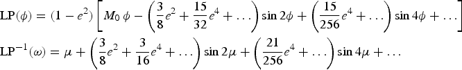 $$\eqalign{&\hbox{LP}\lpar \phi \rpar =\lpar 1-e^2\rpar \left[M_0 \, \phi -\left({\displaystyle{{3}\over{8}}e^2+\displaystyle{{15}\over{32}}e^4+\ldots} \right)\sin 2\phi +\left({\displaystyle{{15}\over{256}}e^4+\ldots} \right)\sin 4\phi +\ldots\right]\cr & \hbox{LP}^{-1}\lpar \omega \rpar =\mu +\left({\displaystyle{{3}\over{8}}e^2+\displaystyle{{3}\over{16}}e^4+\ldots} \right)\sin 2\mu +\left({\displaystyle{{21}\over{256}}e^4+\ldots} \right)\sin 4\mu +\ldots}$$
where
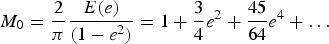 $M_{0} =\displaystyle{{2}\over{\pi}}\displaystyle{{E\lpar e \rpar }\over{\lpar {1-e^{2}} \rpar }} = 1+\displaystyle{{3}\over{4}}e^{2}+\displaystyle{{45}\over{64}}e^{4}+\ldots$
and the rectifying latitude
$M_{0} =\displaystyle{{2}\over{\pi}}\displaystyle{{E\lpar e \rpar }\over{\lpar {1-e^{2}} \rpar }} = 1+\displaystyle{{3}\over{4}}e^{2}+\displaystyle{{45}\over{64}}e^{4}+\ldots$
and the rectifying latitude
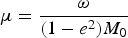 $\mu =\displaystyle{{\omega}\over{\lpar {1-e^{2}}\rpar M_{0}}}$
.
$\mu =\displaystyle{{\omega}\over{\lpar {1-e^{2}}\rpar M_{0}}}$
.
In the case of the sphere LP(ϕ) = ϕ.
Having obtained L 2 and λ2 for position P 2 from Equations (1) and (2) compute the quantity:
 $$\hbox{f}=\sin \delta _2 \sin L_2 +\cos \delta _2 \cos L_2 \cos \lpar {\lambda_2 + \hbox{GHA}_2} \rpar -\cos ZD_2$$
P 2 lies on LoP2 when f(L 1) = 0 and the three conditions listed above will all be satisfied. The starting value L 1 can be adjusted iteratively using standard methods for finding the root of a function of one variable. Convergence is expected to be rapid provided the intersection angle between the LoPs is not too small which is a standard requirement for reliable fixes.
In this procedure the path between P 1 and P 2 is a single rhumb line but it could equally be constructed from multiple rhumb line legs by the repeated application of Equations (1) and (2).
Practical limitations involved in following a precise rhumb line track mean that treating the running fix on the ellipsoid is likely to meet or exceed all real world requirements for accuracy. If it were necessary to go a step further and consider the geoid it would be most natural and efficientFootnote 1 to compute a set of corrections to P 1 and/or P 2 once they have been determined by the method described above. Such additional corrections will not be considered here.
3. AN EXAMPLE
In what follows WGS84 geodetic datum is assumed.
On 29 February 2016 a Sun sight taken at 17:00:00 UT from a ship near latitude 48°N yields ZD
 $_{1}=77^{\circ}36{\cdot}8'$
and for which the Nautical Almanac gives
$_{1}=77^{\circ}36{\cdot}8'$
and for which the Nautical Almanac gives
 $\hbox{GHA}_{1} = 71^{\circ}54{\cdot}3^{^{\prime}}\semicolon \; \delta_{1} = -7^{\circ}36{\cdot}8^{\prime}$
. The Sun's azimuth is
$\hbox{GHA}_{1} = 71^{\circ}54{\cdot}3^{^{\prime}}\semicolon \; \delta_{1} = -7^{\circ}36{\cdot}8^{\prime}$
. The Sun's azimuth is
 $Z_{n} = 117^{\circ}$
.
$Z_{n} = 117^{\circ}$
.
Over the next five hours the vessel travels 50 nautical miles on a course of 160° True at which point a second Sun sight gives ZD
 $_{2}=56^{\circ}13{\cdot}6^{\prime}$
with
$_{2}=56^{\circ}13{\cdot}6^{\prime}$
with
 $\hbox{GHA}_{2} =146^{\circ}54{\cdot}9^{\prime}\semicolon \; \delta_{2} = -7^{\circ}32{\cdot}1^{\prime}$
.
$\hbox{GHA}_{2} =146^{\circ}54{\cdot}9^{\prime}\semicolon \; \delta_{2} = -7^{\circ}32{\cdot}1^{\prime}$
.
For the purposes of illustration it will be assumed that these values are exact.
With these parameters f(47
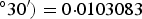 $^{\circ} 30^{\prime}\rpar = 0{\cdot}0103083$
and f(48
$^{\circ} 30^{\prime}\rpar = 0{\cdot}0103083$
and f(48
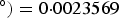 $^{\circ}\rpar = 0{\cdot}0023569$
. With these initial values the solution f(L
1) = 0 can be found by standard iterative methods such as the Secant Method (Press et al. Reference Press, Teukolsky, Vetterling and Flannery2007).
$^{\circ}\rpar = 0{\cdot}0023569$
. With these initial values the solution f(L
1) = 0 can be found by standard iterative methods such as the Secant Method (Press et al. Reference Press, Teukolsky, Vetterling and Flannery2007).
The table below gives the result of iterations performed until successive estimates for P 2 differ by less than 1 metre.
An additional iteration changes the position of P
2 by 2 μm. The locations of P
2 obtained by assuming a sphere (e = 0) and WGS84 ellipsoid (
 $e = 0{\cdot}08181919\ldots$
) differ by 4·4 m. Convergence is rapid as the LoPs are fairly straight over the scale of this problem.
$e = 0{\cdot}08181919\ldots$
) differ by 4·4 m. Convergence is rapid as the LoPs are fairly straight over the scale of this problem.
The result
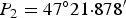 $P_{2} = 47^{\circ}21{\cdot}878^{\prime}$
N, 133
$P_{2} = 47^{\circ}21{\cdot}878^{\prime}$
N, 133
 $^{\circ}12{\cdot}958^{\prime}$
W is the required fix at the time of the second celestial sight. The vessel's position at the time of the first sight
$^{\circ}12{\cdot}958^{\prime}$
W is the required fix at the time of the second celestial sight. The vessel's position at the time of the first sight
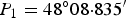 $P_{1} = 48^{\circ} 08{\cdot}835^{\prime}$
N, 133
$P_{1} = 48^{\circ} 08{\cdot}835^{\prime}$
N, 133
 $^{\circ}38{\cdot}303^{\prime}$
W is also obtained as a by-product without additional computational effort. The positions P
1 and P
2 satisfy the three conditions listed in the text are therefore consistent with all available information including the vessel's distance and direction of travel. A graphical representation of the results of the procedure is shown in Figure 2.
$^{\circ}38{\cdot}303^{\prime}$
W is also obtained as a by-product without additional computational effort. The positions P
1 and P
2 satisfy the three conditions listed in the text are therefore consistent with all available information including the vessel's distance and direction of travel. A graphical representation of the results of the procedure is shown in Figure 2.

Figure 2. The iterative procedure described in the text finds points P 1 and P 2 lying on LoP1 and LoP2 respectively and separated by a specified rhumb line distance of (50 nautical miles) and bearing (160° True). The dotted arrows are the initial trials used in Iteration 0 of Table 1. These satisfy 1) and 2) of the conditions listed in the text but not 3). Since LoP1 is not advanced it does not undergo the distortion illustrated in Figure 1 and therefore retains its relatively simple algebraic form.
Table 1. Successive estimates of latitude. L, and longitude, λ, of positions P 1 and P 2 in solving the equation f(L 1) = 0. The column labelled ΔP 2 gives the change in the location of P 2 compared to the previous estimate inmetres.

4. CONCLUSIONS
In a running fix two celestial sights and the known track of the vessel provide three key pieces of information or conditions that must be satisfied for the fix to be valid. It has been shown that the solution to this problem can be reduced to one of finding the root of a well-behaved function in one variable and that standard iterative methods can be applied to determine the root to arbitrary accuracy. The procedure yields the unique position that is consistent with all the available information and is applicable to both the sphere and ellipsoid. The need to advance the initial LoP with its associated complexities and ambiguities is avoided.


