


1. INTRODUCTION
The Global Positioning System (GPS) is a satellite-based navigation system that provides a user access to useful and accurate positioning information anywhere on the globe (Axelrad and Brown, Reference Axelrad, Brown, Parkinson, Spilker, Axelrad and Enga1996). The well-known Kalman Filter (KF) (Gelb, Reference Gelb1974; Brown and Hwang, Reference Brown and Hwang1997), which provides an optimal (minimum mean square error) estimate of the system state vector, has been widely applied to the field of navigation.
In navigation filter processing, the linear model increases modelling errors since the vehicle motions are normally nonlinear. It has been common that additional fictitious process noise can be added to the system process model, nevertheless, the more suitable cure for the divergence problem caused by mis-modelling is to correct the dynamics model. To achieve improved estimation accuracy, the designers are required to possess complete a priori knowledge on both the dynamic process and measurement models. The Extended Kalman Filter (EKF) relies on the first order linearization of the system model to propagate the mean and covariance of the state. The EKF is sensitive to outliers in the measurements, thus it is likely to yield poor performance if the measurements include outliers.
The Unscented Kalman Filter (UKF) (Julier, Reference Julier2002; Julier et al., Reference Julier, Uhlmann and Durrant-Whyte1995; Julier et al., Reference Julier, Uhlmann and Durrant-Whyte2000) has been developed to deal with highly nonlinear state estimation problems. The UKF performs a Gaussian approximation with a limited number of points (sigma points) using the Unscented Transform (UT). The sigma points are used to propagate the probability of state distribution through the nonlinear dynamics of the system. The standard EKF is generally a first order approximation, whereas the EKF based on a second-order Taylor expansion is shown to be quite closely related to UKF. Gustafsson and Hendeby (Reference Gustafsson and Hendeby2012) indicated that the UT gives a good approximation of many standard sensor models in tracking and navigation applications, however, UT generally does not give the same elements in the covariance as the second-order Taylor expansion. A simple counterexample was demonstrated in Gustafsson and Hendeby (Reference Gustafsson and Hendeby2012). Furthermore, for high-dimensional systems, the UT or the UKF is believed to be unstable due to the possible negative weights on the centre point.
As a general approach to approximating the Bayesian solution, the Cubature Kalman Flter (CKF) proposed by Arasaratnam and Haykin (Reference Arasaratnam and Haykin2009) has been an increasing interest in the development of nonlinear Bayesian filters. The CKF uses a third-degree spherical-radial cubature rule to solve the integration in the Bayesian filtering problem for numerically computing the multivariate moment integrals encountered in the nonlinear filtering framework. The CKF is considered to be a more accurate and stable nonlinear filtering approach than the UKF and has been used in many engineering applications (Fernandez-Prades and Vila-Valls, Reference Fernandez-Prades and Vila-Valls2010). The spherical-radial cubature rule is composed of two different integrals which include spherical and radial integrals. This is based on the spherical-radial transformation and generates an even number of equally weighted cubature points. These integrals are then numerically computed by the spherical cubature rule and the Gaussian quadrature rule, respectively. The performance in terms of estimation accuracy, numerical stability and computational costs can be improved.
Gustafsson and Hendeby (Reference Gustafsson and Hendeby2012) pointed out that the CKF can be viewed as a special case of UKF. The viewpoint provided by Wu et al. (Reference Wu, Hu, Wu and Hu2006) has validated the statement. As stated in this paper, the UT is essentially a Gaussian quadrature rule and other similar rules can also be applied. The spherical-radial cubature rule used in CKF is a special case of the quadrature rules. The higher-degree CKF was studied in Jia et al. (Reference Jia, Xin and Cheng2013), and higher-order UKF has already been studied in Wu et al. (Reference Wu, Hu, Wu and Hu2006). The possible negative weights of the centre point in UT can be avoided through tuning the parameters (Julier et al., Reference Julier, Uhlmann and Durrant-Whyte2000). Using the additional tuning parameters of UKF compared to CKF provides flexibility. If one does not want to bother to tune them, we can fix them as their default values, or just exclude the centre point, and the CKF is automatically obtained.
The differences between UKF and CKF are summarised as follows: (1) The CKF uses cubature points with the same weights through the spherical-radial integration rule, which employs an analytical Probability Density Function (PDF) to capture the mean and covariance of the posterior distribution using the total probability theorem and subsequently uses the measurement to update with Bayes' rule. From the perspective of numerical analysis, the third-degree cubature rule can be viewed as a UT of special form with better numerical stability; (2) the CKF follows directly from the spherical-radial cubature rule for numerically computing Gaussian-weighted integrals whose important property is that they do not entail any free parameters. The UKF introduces a non-zero scaling parameter, which defines the non-zero centre point and is often associated with a set of weighted samples higher than that of the minimal set of sigma points (Julier et al., Reference Julier, Uhlmann and Durrant-Whyte1995; Wan and Van der Merwe, Reference Wan, Van der Merwe and Haykin2001; Van der Merwe and Wan, Reference Van der Merwe and Wan2004); (3) the UKF-calculated estimation covariance matrix is not always guaranteed to be positive definite, hence the decomposition of the covariance matrix is unavailable. To improve the stability of the nonlinear filter, the CKF can effectively avoid round-off errors of numerical computation, and it is more stable than the UKF and EKF (Jia et al., Reference Jia, Xin and Cheng2013).
Investigation of the CKF algorithm on the navigation problem presented by Xu et al. (Reference Xu, Xiao, Gao, Zhang, Liu and Liu2014) assumed that the Kalman-type filters are concerned with estimation of the dynamics model from noisy measurements where the dynamic and measurement processes can be approximated by Gaussian state-space models. Those nonlinear filters are very sensitive to measurement errors when the distribution of the true noise deviates from the assumed Gaussian model, often being characterised by high-intensity measurement noise and heavy tail distributions. There is considerable motivation to consider robust statistical procedures to improve the performance of the CKF in non-Gaussian environments, particularly in the presence of outliers.
Masreliez and Martin (Reference Masreliez and Martin1977) used the M-estimator to “robustify” the KF. Boncelet and Dickinson (Reference Boncelet and Dickinson1983) recast the measurement update as a linear regression problem and solved it using the M-estimator. Using the M-estimator, Yang (Reference Yang1991) robustified the general Bayes estimator by which KF had been seen as a special case. An adaptively Robust Kalman Filter (RKF), capable of dealing with uncertainties in both process and measurement models, was proposed in Yang et al. (Reference Yang, He and Xu2001) and Yang and Gao (Reference Yang and Gao2006a; Reference Yang and Gao2006b), in which the influences of measurement outliers were controlled using the M-estimator. The Sigma Point Kalman Filter (SPKF) was robustified by Karlgaard et al. (Reference Karlgaard, Schaub, Crassidis, Psiaki, Chiang, Ohlmeyer and Norgaard2007), focusing on the divided difference filter. As the statistical linearization perspective of the UT is incorrectly employed in the work by Karlgaard et al. (Reference Karlgaard, Schaub, Crassidis, Psiaki, Chiang, Ohlmeyer and Norgaard2007) and Wang et al. (Reference Wang, Cui and Guo2010), Chang et al. (Reference Chang, Hu, Chang and Li2012a) robustified the measurement update of the UKF using the M-estimator in a straightforward and intuitive manner. Recently, the robust sigma point Kalman smoother was studied by Karlgaard (Reference Karlgaard2015). It should be noted that two kinds of nonlinearity exist, i.e., the original nonlinearity in the measurement equation, and that brought by the re-weighting procedure of the M-estimator, and the iteration becomes rather complex. If both nonlinearities were to be accounted for in the iteration, it involves issues of iterative UKF (Chang et al., Reference Chang, Hu, Chang and Li2012b; Reference Chang, Hu, Chang and Li2012c).
The Huber M-estimation methodology (Huber, Reference Huber1981; Maronna et al., Reference Maronna, Martin and Yohai2006; Gandhi and Mili, Reference Gandhi and Mili2010; Chang and Liu, Reference Chang and Liu2015) is one of the robust techniques that is based on the combination of minimum ℓ1 – and ℓ2 – norm estimator. The method has been successfully used for robust state estimation, inertial navigation system and visual tracking applications (Wang et al., Reference Wang, Cui and Guo2010; Gao et al., Reference Gao, Liu and Xu2014; Hou, Reference Hou2014). The development of a RKF uses the Huber technique applied to a linear regression problem at each measurement update (Kovacevic et al. Reference Kovacevic, Durovic and Glavaski1992; Durgaprasad and Thakur, Reference Durgaprasad and Thakur1998). The Huber M-estimation methodology is essentially based on modifying the quadratic cost function in the filter framework, and works between smooth ℓ2 – norm properties for small residuals and robust ℓ1 – norm properties for large residuals (Petrus, Reference Petrus1999). Alternative functional equations, such as the Huber criterion and the hybrid ℓ1/ℓ2 criterion have also been considered (Huber, Reference Huber1973; Bube and Langan, Reference Bube and Langan1997; Guitton and Symes, Reference Guitton and Symes2003).
The robust Huber-based Cubature Kalman Filter (HCKF) algorithm integrates the merits of the Huber M-estimation methodology and CKF. The CKF is used to avoid the numerical instability and the Huber M-estimation methodology is incorporated to handle outliers through reformulating the measurement information in the CKF framework to provide robustness against deviations from Gaussian behaviour.
This paper is organised as follows. In Section 2, the preliminary background to the nonlinear filter is introduced, where the UKF and the CKF will be reviewed. The Huber M-estimate regression filtering strategy is presented in Section 3. In Section 4, some results from simulation and experiments are presented to evaluate GPS navigation performance for the HCKF approach in comparison to those by the conventional approach. Conclusions are given in Section 5.
2. THE NONLINEAR FILTERS
The nonlinear filtering deals with the case governed by the nonlinear stochastic difference equations:
 $${\bf x}_{k + 1} = {\bf f}({\bf x}_k, k) + {\bf w}_k $$
 $${\bf z}_k = {\bf h}({\bf x}_k, k) + {\bf v}_k $$
where the state vector is ${\bf x}_k \in \Re ^n {\rm } $
, process noise vector
${\bf x}_k \in \Re ^n {\rm } $
, process noise vector ${\bf w}_k \in \Re ^n $
, measurement vector
${\bf w}_k \in \Re ^n $
, measurement vector ${\bf z}_k \in \Re ^m $
, and measurement noise vector
${\bf z}_k \in \Re ^m $
, and measurement noise vector ${\bf v}_k \in \Re ^m $
. The vectors
${\bf v}_k \in \Re ^m $
. The vectors ${\bf w}_k $
and
${\bf w}_k $
and ${\bf v}_k $
are zero mean Gaussian white sequences having zero cross-correlation with each other:
${\bf v}_k $
are zero mean Gaussian white sequences having zero cross-correlation with each other:
 $${\bf E}[{\bf w}_k {\bf w}_i^{\rm T} ] = \left\{ {\matrix{ {{\bf Q}_k, \matrix{ {} & {i = k} \cr}} \cr {0,\matrix{ {} & {i \ne k} \cr}} \cr}} \right.;\ {\bf E}[{\bf v}_k {\bf v}_i^{\rm T} ] = \left\{ {\matrix{ {{\bf R}_k, \matrix{ {} & {i = k} \cr}} \cr {0,\matrix{ {} & {i \ne k} \cr}} \cr}} \right.;\ {\bf E}[{\bf w}_k {\bf v}_i^{\rm T} ] = {\bf 0}\quad \quad for\;all\;i\;and\;k$$
where ${\bf Q}_k $
is the process noise covariance matrix,
${\bf Q}_k $
is the process noise covariance matrix, ${\bf R}_k $
is the measurement noise covariance matrix.
${\bf R}_k $
is the measurement noise covariance matrix.
2.1. Unscented Kalman Filter
The first step in the UKF involves the UT to generate a set of weighted samples/sigma points, which are deterministically chosen so that they adequately capture the true mean and covariance of the random variable. Consider an n dimensional random variable ${\bf x}$
, which has the mean
${\bf x}$
, which has the mean $\hat {\bf x}$
and covariance
$\hat {\bf x}$
and covariance ${\bf P}$
, and suppose that it propagates through an arbitrary nonlinear function
${\bf P}$
, and suppose that it propagates through an arbitrary nonlinear function ${\bf f}$
. The UT creates 2n + 1 sigma vectors
${\bf f}$
. The UT creates 2n + 1 sigma vectors ${\bf x}$
(a capital letter) and weighted points W,
${\bf x}$
(a capital letter) and weighted points W,
 $${\bf X}_{(0)} = \hat {\bf x};\,{\bf X}_{(i)} = \hat {\bf x} + (\sqrt {(n + \lambda ){\bf P}} )_i^T ;{\bf X}_{(i + n)} = \hat {\bf x} - (\sqrt {(n + \lambda ){\bf P}} )_i^T, i = 1,...,n$$
 $$\eqalign{W_0^{(m)} &= \displaystyle{\lambda \over {(n + \lambda )}};\,W_0^{(c)} = W_0^{(m)} + (1 - \alpha ^2 + \beta );\,W_i^{(m)} = W_i^{(c)} = \displaystyle{1 \over {2(n + \lambda )}}, \cr i &= 1\comma\ldots\comma \,2n\,}$$
where ${\bf (}\sqrt {{\bf (}n + \lambda {\bf )P}} {\bf )}_i $
is the ith row of the matrix square root.
${\bf (}\sqrt {{\bf (}n + \lambda {\bf )P}} {\bf )}_i $
is the ith row of the matrix square root. $\sqrt {{\bf (}n + \lambda {\bf )P}} $
can be obtained from the lower-triangular matrix of the Cholesky factorisation;
$\sqrt {{\bf (}n + \lambda {\bf )P}} $
can be obtained from the lower-triangular matrix of the Cholesky factorisation; $\lambda = \alpha ^2 (n + \kappa ) - n$
is a scaling parameter; α determines the spread of the sigma points around
$\lambda = \alpha ^2 (n + \kappa ) - n$
is a scaling parameter; α determines the spread of the sigma points around ${\mathop{\bf x}\limits^{\frown}}$
; κ is a secondary scaling parameter; β is used to incorporate prior knowledge of the distribution of
${\mathop{\bf x}\limits^{\frown}}$
; κ is a secondary scaling parameter; β is used to incorporate prior knowledge of the distribution of $\bar {\bf x}$
;
$\bar {\bf x}$
; $W_i^{(m)} $
and
$W_i^{(m)} $
and $W_i^{(c)} $
are the weights for the mean and covariance, respectively, associated with the ith point.
$W_i^{(c)} $
are the weights for the mean and covariance, respectively, associated with the ith point.
The sigma vectors are propagated through the nonlinear function to yield a set of transformed sigma points,
 $${\bf y}_i = f\,({\bf X}_i )\,i = 0,...,2n$$
The mean and covariance of ${\bf y}_i $
are approximated by a weighted average mean and covariance of the transformed sigma points:
${\bf y}_i $
are approximated by a weighted average mean and covariance of the transformed sigma points:
 $$\bar {\bf y}_u = \sum\limits_{i = 0}^{2n} {W_i^{(m)}} {\bf y}_i $$
 $${\bf P}_u = \sum\limits_{i = 0}^{2n} {W_i^{(c)}} ({\bf y}_i - \bar {\bf y}_u )({\bf y}_i - \bar {\bf y}_u )^T $$
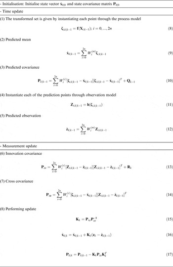
To implement the UKF, the set of sigma points are firstly created by Equation (3). After that, the algorithm for implementation of the UKF is summarized in Table 1 (Tseng et al., Reference Tseng, Lin and Jwo2016). The UKF involves the time update (prediction) stage, i.e., Equations (8)–(12), and the measurement update (correction) stage, i.e., Equations (13)–(17).
Table 1. Implementation algorithm for the unscented Kalman filter.
2.2. The Cubature Kalman Filter
Like the UKF, the CKF is another type of nonlinear filtering approach without linearization of the nonlinear model. The first step of the CKF algorithm is to approximate the mean and variance of the probability distribution through a set of 2n (n is the dimension of the system model) cubature points. The cubature points are then propagated through the nonlinear functions. The mean and variance of the current approximate Gaussian distribution by the propagated cubature points can then be calculated. A set of 2n cubature points are given by $[{\bf \xi} _i, {\rm } \omega _i ]$
, where
$[{\bf \xi} _i, {\rm } \omega _i ]$
, where ${\bf \xi} _i $
is the ith cubature point and ω
i
is the corresponding weight:
${\bf \xi} _i $
is the ith cubature point and ω
i
is the corresponding weight:
 $${\bf \xi} _i = \left\{ {\matrix{ {\sqrt n [1]_i, {\rm}} \cr { - \sqrt n [1]_{i - n}, {\rm}} \cr}} \right.{\rm} \matrix{ {i = 1,2,...,n} \hfill \cr {i = n + 1,n + 2,...,2n} \hfill \cr} \,{\rm ;}\ \omega _i = \displaystyle{1 \over {2n}},{\rm} i = 1,2,...,2n$$
where $\left[ 1 \right]_i \in \Re ^n $
denotes the ith column vector of the identity matrix I
n×n
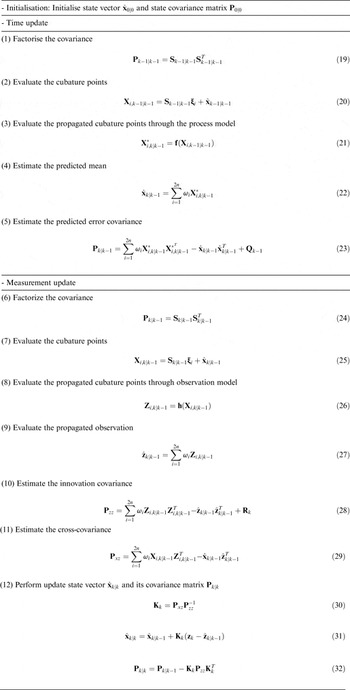
. Under the assumption that the posterior density at time k – 1 is known, the steps involved in the time and measurement updates are given by Equations (19)–(32), summarised in Table 2. See Tseng et al. (Reference Tseng, Lin and Jwo2016) for further discussion.
$\left[ 1 \right]_i \in \Re ^n $
denotes the ith column vector of the identity matrix I
n×n
. Under the assumption that the posterior density at time k – 1 is known, the steps involved in the time and measurement updates are given by Equations (19)–(32), summarised in Table 2. See Tseng et al. (Reference Tseng, Lin and Jwo2016) for further discussion.
Table 2. Implementation algorithm for the cubature Kalman filter.
3. THE HUBER-BASED REGRESSION FILTERING STRATEGY
As a recursive minimum ℓ2 – norm estimation technique, the KF exhibits sensitivity to deviations from the assumed underlying probability distributions.
3.1. The Huber M-estimate regression filtering
The technique that relies on Huber's generalised Maximum Likelihood (ML) methodology exhibits robustness against deviations from the commonly assumed Gaussian probability density functions and can solve the non-Gaussian distribution problem efficiently. The measurement update can be modified to enhance robustness using the Huber M-estimation methodology.
To incorporate this mechanism into the CKF framework, it is necessary to reformulate the measurement update as a nonlinear regression problem between the state prediction and the observed quantity, and then the nonlinear regression model has the form (Chang et al., Reference Chang, Hu, Chang and Li2012a; Tsakonas et al., Reference Tsakonas, Jaldén, Sidiropoulos and Ottersten2014)
 $$\left[ {\matrix{ {{\bf z}_k} \cr {\hat {\bf x}_{k \vert k - 1}} \cr}} \right] = \left[ {\matrix{ {{\bf h}({\bf x}_k )} \cr {{\bf x}_k} \cr}} \right] + \left[ {\matrix{ {{\bf v}_k} \cr {\delta {\bf x}_k} \cr}} \right]$$
where ${\bf z}_k $
is the measurement;
${\bf z}_k $
is the measurement; $\hat {\bf x}_{k \vert k - 1} $
is the predicted state, which is obtained from the time update of the CKF, and
$\hat {\bf x}_{k \vert k - 1} $
is the predicted state, which is obtained from the time update of the CKF, and $\delta {\bf x}_k $
is the error between the true state and its prediction. Denote
$\delta {\bf x}_k $
is the error between the true state and its prediction. Denote
 $${\bf e}_k = \left[ {\matrix{ {{\bf v}_k} \cr {\delta {\bf x}_k} \cr}} \right]{\rm}$$
with
 $$E[{\bf e}_{\bf k} ] = 0{\rm} \,{\rm and}\,{\rm} E[{\bf e}_k {\bf e}_k^T ] = \left[ {\matrix{ {{\bf R}_k} & {\bf 0} \cr {\bf 0} & {{\bf P}_{k \vert k - 1}} \cr}} \right] = {\bf \Lambda} _k {\bf \Lambda} _k^T $$
where the term ${\bf \Lambda} _k $
may be obtained by Cholesky decomposition,
${\bf \Lambda} _k $
may be obtained by Cholesky decomposition, ${\bf R}_k $
is assumed to be a known noise covariance of
${\bf R}_k $
is assumed to be a known noise covariance of ${\bf v}_k $
, and
${\bf v}_k $
, and ${\bf P}_{k \vert k - 1} $
is the error covariance propagation.
${\bf P}_{k \vert k - 1} $
is the error covariance propagation.
Multiplying Equation (33) with ${\bf \Lambda} _k^{ - 1} $
yields the nonlinear regression model
${\bf \Lambda} _k^{ - 1} $
yields the nonlinear regression model
 $$\tilde {\bf z}_k = {\bf g}({\bf x}_k ) + {\bf \upsilon} _k $$
where
 $$\tilde {\bf z}_k = {\bf \Lambda} _k^{ - 1} \left[ {\matrix{ {{\bf z}_k} \cr {\hat {\bf x}_{k \vert k - 1}} \cr}} \right]$$
and
 $${\bf g}({\bf x}_k ) = {\bf \Lambda} _k^{ - 1} \left[ {\matrix{ {{\bf h}({\bf x}_k )} \cr {{\bf x}_k} \cr}} \right];\,{\bf \upsilon} _k = {\bf \Lambda} _k^{ - 1} \left[ {\matrix{ {{\bf v}_k} \cr {\delta {\bf x}_k} \cr}} \right]\,$$
The covariance matrix of ${\bf \upsilon} _k $
is the identity matrix, as can be seen from expanding the expectation
${\bf \upsilon} _k $
is the identity matrix, as can be seen from expanding the expectation $E[{\bf \upsilon} _k {\bf \upsilon} _k^T ]$
.
$E[{\bf \upsilon} _k {\bf \upsilon} _k^T ]$
.
In Equation (35), the nonlinear regression problem can be solved efficiently for robustness using Huber's generalised ML method, in which the solution is found by minimising the cost function
 $$\hat {\bf x}_{k \vert k} = \arg \min \sum\limits_{i = 1}^{m + n} {\rho (\upsilon _{k,i} )}$$
where υ
k,i
is the ith component of the residual vector, ${\bf \upsilon} _k $
, and
${\bf \upsilon} _k $
, and $\rho ( \cdot )$
is the score function used to handle the outlier measurements or contaminated Gaussian; m is the dimension of the measurement. The Huber ρ – function used in the M-estimation is given by
$\rho ( \cdot )$
is the score function used to handle the outlier measurements or contaminated Gaussian; m is the dimension of the measurement. The Huber ρ – function used in the M-estimation is given by
 $$\rho (\upsilon _{k,i} ) = \left\{ {\matrix{ {\displaystyle{1 \over 2}\upsilon _{k,i}^2} \cr {\gamma \vert \upsilon _{k,i} \vert - \displaystyle{1 \over 2}\gamma ^2} \cr}} \right.\,\matrix{ {{\rm for} \vert \upsilon _{k,i} \vert \lt \gamma} \cr {{\rm for} \vert \upsilon _{k,i} \vert \ge \gamma} \cr} \,$$
where γ is a tuning parameter. The ρ function is a blend of the ℓ1 – and ℓ2 – norm estimation functions, which provides ℓ2 – norm properties for small residuals to ensure both quality and efficiency simultaneously with normal distribution and ℓ1 – norm properties for large residuals to suppress the impact of outliers or contaminated Gaussian noises.
If the ρ – function is differentiable, the solution to the nonlinear regression problem can be found by deriving the cost function as
 $$\sum\limits_{i = 1}^{m + n} {\phi (\upsilon _{k,i} )} \displaystyle{{\partial \upsilon _{k,i}} \over {\partial {\bf x}_k}} = 0 $$
where $\phi (\upsilon _{k,i} ) = \rho '(\upsilon _{k,i} )$
. By defining the ψ – function as
$\phi (\upsilon _{k,i} ) = \rho '(\upsilon _{k,i} )$
. By defining the ψ – function as $\psi (\upsilon _{k,i} ) = \phi (\upsilon _{k,i} )/\upsilon _{k,i} $
, and corresponding to the Huber density
$\psi (\upsilon _{k,i} ) = \phi (\upsilon _{k,i} )/\upsilon _{k,i} $
, and corresponding to the Huber density
 $$\psi (\upsilon _{k,i} ) = \left\{ {\matrix{ 1 \cr {\gamma {\mathop{\rm sgn}} (\upsilon _{k,i} )/\upsilon _{k,i}} \cr}} \right.\,\matrix{ {{\rm for} \vert \upsilon _{k,i} \vert \le \gamma} \cr {{\rm for} \vert \upsilon _{k,i} \vert \gt \gamma} \cr} $$
The Huber M-estimation methodology makes use of the weighting matrix ${\bf \Psi} _k = {\rm diag}[\psi (\upsilon _{k,i} )]$
to recast the measurement information. The weighting matrix
${\bf \Psi} _k = {\rm diag}[\psi (\upsilon _{k,i} )]$
to recast the measurement information. The weighting matrix ${\bf \Psi} _k $
can be interpreted in terms of re-weighting the residual error covariance and constructing the measurement process. The modified covariance is given by
${\bf \Psi} _k $
can be interpreted in terms of re-weighting the residual error covariance and constructing the measurement process. The modified covariance is given by
 $$\bar {\bf S}_k = {\bf \Lambda} _k^{1/2} {\bf \Psi} _k^{ - 1} {\bf \Lambda} _k^{T/2} $$
The decomposition of the $\bar {\bf S}_k $
matrix into two submatrices
$\bar {\bf S}_k $
matrix into two submatrices $\bar {\bf S}_{k,x} $
and
$\bar {\bf S}_{k,x} $
and $\bar {\bf S}_{k,z} $
corresponding to the state update and state correction with measurements so that
$\bar {\bf S}_{k,z} $
corresponding to the state update and state correction with measurements so that
 $$\bar {\bf S}_k = \left[ {\matrix{ {\bar {\bf S}_{k,z}} & 0 \cr 0 & {\bar {\bf S}_{k,x}} \cr}} \right]$$
where the $\bar {\bf S}_{k,x} \in \Re ^{n \times n} $
and
$\bar {\bf S}_{k,x} \in \Re ^{n \times n} $
and $\bar {\bf S}_{k,z} \in \Re ^{m \times m} $
, and the robust measure of correlation can be expressed in the recursive filter as the CKF measurement-update.
$\bar {\bf S}_{k,z} \in \Re ^{m \times m} $
, and the robust measure of correlation can be expressed in the recursive filter as the CKF measurement-update.
3.2. The Huber M-estimation methodology-based cubature Kalman filter
The Huber M-estimation methodology is robust to the outliers and ensures the accuracy of the state estimation. To apply this method, the ψ – function is the component of the residual vector ${\bf \upsilon} _k $
. Specifically, when |υ
k,i
| ≤ γ, the accurate estimation of the system state reaches the expected behaviour demand and Huber-based filtering is equal to the CKF measurement update because
${\bf \upsilon} _k $
. Specifically, when |υ
k,i
| ≤ γ, the accurate estimation of the system state reaches the expected behaviour demand and Huber-based filtering is equal to the CKF measurement update because ${\bf \Psi} _k = {\bf I}$
. On the other hand, when |υ
k,i
| > γ, the CKF has a divergent trend due to the noisy signal contaminated with outliers. The measurement update is modified to exhibit robustness using the Huber M-estimation methodology. Defining
${\bf \Psi} _k = {\bf I}$
. On the other hand, when |υ
k,i
| > γ, the CKF has a divergent trend due to the noisy signal contaminated with outliers. The measurement update is modified to exhibit robustness using the Huber M-estimation methodology. Defining
 $$\tilde {\bf R}_k = \bar {\bf S}_{k,z} $$
as the modified measurement covariance, and replacing ${\bf R}_k $
with
${\bf R}_k $
with $\tilde {\bf R}_k $
for operating the CKF framework in the measurement update process leads to the HCKF.
$\tilde {\bf R}_k $
for operating the CKF framework in the measurement update process leads to the HCKF.
The M-estimation problem in Huber-based regression filtering aims to minimise Equation (38), which is essentially nonlinear. In general, the calculation procedure of the RKF based on the M-estimation should be solved iteratively because the reweight matrix is constructed based on the residuals which are further related to the state parameter estimates. By setting the weighting matrix ${\bf \Psi} _k = {\rm diag}[\psi (\upsilon _{k,i} )]$
, an iterative solution to Equation (40) can be obtained using statistical approximation of the nonlinear function
${\bf \Psi} _k = {\rm diag}[\psi (\upsilon _{k,i} )]$
, an iterative solution to Equation (40) can be obtained using statistical approximation of the nonlinear function ${\bf M}_k ( \cdot )$
. The implicit Equation (40) can be written in matrix form,
${\bf M}_k ( \cdot )$
. The implicit Equation (40) can be written in matrix form,
 $${\bf M}_k^T {\bf \Psi} _k ({\bf M}_k x_k - \tilde {\bf z}_k ) = 0 $$
which can be solved for ${\bf x}_k $
to give
${\bf x}_k $
to give ${\bf x}_k = ({\bf M}_k^T {\bf \Psi} _k {\bf M}_k )^{ - 1} {\bf M}_k^T {\bf \Psi} _k \tilde {\bf z}_k $
. An iterative solution to Equation (45) is expressed as
${\bf x}_k = ({\bf M}_k^T {\bf \Psi} _k {\bf M}_k )^{ - 1} {\bf M}_k^T {\bf \Psi} _k \tilde {\bf z}_k $
. An iterative solution to Equation (45) is expressed as
 $${\bf x}_k^{(\,j + 1)} = ({\bf M}_k^T {\bf \Psi} _k^{(\,j)} {\bf M}_k )^{ - 1} {\bf M}_k^T {\bf \Psi} _k^{(\,j)} \tilde {\bf z}_k $$
where the superscript $(j)$
is the iteration index. The method can be initialised using the iteratively reweighted least squares solution:
$(j)$
is the iteration index. The method can be initialised using the iteratively reweighted least squares solution: ${\bf x}_k^{(0)} = ({\bf M}_k^T {\bf M}_k )^{ - 1} {\bf M}_k^T \tilde {\bf z}_k $
. The iteration will converge if the ψ function is non-increasing when using the Huber ρ function. The Huber M-estimation methodology can be iterated until convergence or can be carried out through only one fixed iteration step to save the computational costs.
${\bf x}_k^{(0)} = ({\bf M}_k^T {\bf M}_k )^{ - 1} {\bf M}_k^T \tilde {\bf z}_k $
. The iteration will converge if the ψ function is non-increasing when using the Huber ρ function. The Huber M-estimation methodology can be iterated until convergence or can be carried out through only one fixed iteration step to save the computational costs.
The one-step Huber update is summarised as follows: (1) Calculate ${\bf X}_{i,k \vert k - 1} $
,
${\bf X}_{i,k \vert k - 1} $
, ${\bf Z}_{i,k \vert k - 1} $
and
${\bf Z}_{i,k \vert k - 1} $
and $\hat {\bf z}_{k \vert k - 1} $
using Equations (24)–(27); (2) Form a redundant observation vector shown as in Equation (33); (3) Solve the nonlinear regression model, Equation (35), using the solution based on Equation (46); (4) Update the modified covariance matrix using Equation (42); (5) Perform the modified measurement covariance
$\hat {\bf z}_{k \vert k - 1} $
using Equations (24)–(27); (2) Form a redundant observation vector shown as in Equation (33); (3) Solve the nonlinear regression model, Equation (35), using the solution based on Equation (46); (4) Update the modified covariance matrix using Equation (42); (5) Perform the modified measurement covariance $\tilde {\bf R}_k = \bar {\bf S}_{k,z} $
, and replace
$\tilde {\bf R}_k = \bar {\bf S}_{k,z} $
, and replace ${\bf R}_k $
with
${\bf R}_k $
with $\tilde {\bf R}_k $
for operating the CKF framework in Equation (28). A high level operation of the HCKF is shown in Figure 1(a). Figure 1(b) presents the architecture of the GPS navigation processing using the HCKF implementation. The block indicated by the dashed-line is the Huber M-estimation mechanism for reformulating the measurement information of the CKF framework.
$\tilde {\bf R}_k $
for operating the CKF framework in Equation (28). A high level operation of the HCKF is shown in Figure 1(a). Figure 1(b) presents the architecture of the GPS navigation processing using the HCKF implementation. The block indicated by the dashed-line is the Huber M-estimation mechanism for reformulating the measurement information of the CKF framework.
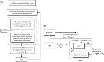
Figure 1. (a) High level operation of the HCKF. (b) Configuration of the GPS navigation processing using the HCKF.
4. GPS NAVIGATION PROCESSING AND PERFORMANCE EVALUATION
Both the Position-Velocity (PV) model and the Position-Velocity-Acceleration (PVA) model are linear. The nonlinear dynamic model that provides more adequate description of the vehicle is adopted from Jwo and Lai (Reference Jwo and Lai2008).
4.1. Nonlinear dynamic modelling for GPS navigation
Consider a vehicle moving at the velocity represented as ${\bf V}_b = u_b {\vec i} + v_b {\vec j} + w_b {\vec k}$
. The velocity in the fixed frame in terms of Euler angles and body velocity components has the relation
${\bf V}_b = u_b {\vec i} + v_b {\vec j} + w_b {\vec k}$
. The velocity in the fixed frame in terms of Euler angles and body velocity components has the relation
 $${\bf V}_b = \left[ {\matrix{ {\dot x} \cr {\dot y} \cr {\dot z} \cr}} \right] = \left[ {\matrix{ {C_\theta C_\psi} & {S_\Phi S_\theta C_\psi - C_\Phi S_\psi} & {C_\Phi S_\theta C_\psi + S_\Phi S_\psi} \cr {C_\theta S_\psi} & {S_\Phi S_\theta S_\psi + C_\Phi C_\psi} & {C_\Phi S_\theta S_\psi - S_\Phi C_\psi} \cr { - S_\theta} & {S_\Phi C_\theta} & {C_\Phi C_\theta} \cr}} \right]\left[ {\matrix{ {u_b} \cr {v_b} \cr {w_b} \cr}} \right]$$
where the following notations are used: $S_\Phi \equiv \sin (\Phi )$
,
$S_\Phi \equiv \sin (\Phi )$
, $C_\Phi \equiv \cos (\Phi )$
,
$C_\Phi \equiv \cos (\Phi )$
, $S_\theta \equiv \sin (\theta )$
,
$S_\theta \equiv \sin (\theta )$
, $C_\theta \equiv \cos (\theta )$
,
$C_\theta \equiv \cos (\theta )$
, $S_\psi \equiv \sin (\psi )$
, and
$S_\psi \equiv \sin (\psi )$
, and $C_\psi \equiv \cos (\psi )$
. Suppose that the non-holonomic constraint is applied, only the longitudinal movement is considered and the lateral slippage is neglected. In case the velocity in the x-component of the body frame is considered,
$C_\psi \equiv \cos (\psi )$
. Suppose that the non-holonomic constraint is applied, only the longitudinal movement is considered and the lateral slippage is neglected. In case the velocity in the x-component of the body frame is considered, $\vert\vert{\bf V}_b \vert\vert \approx \vert\vert u_b \vec i\vert\vert \approx V$
, the dynamic process model of the GPS receiver, when written in the form
$\vert\vert{\bf V}_b \vert\vert \approx \vert\vert u_b \vec i\vert\vert \approx V$
, the dynamic process model of the GPS receiver, when written in the form $ \dot {\bf x} = {\bf f}({\bf x},t) + {\bf u}(t)$
, can be represented as
$ \dot {\bf x} = {\bf f}({\bf x},t) + {\bf u}(t)$
, can be represented as
 $$\left[ {\matrix{ {\dot x} \cr {\dot y} \cr {\dot z} \cr {\dot \Phi} \cr {\dot \theta} \cr {\dot \psi} \cr {\dot V} \cr {\dot b} \cr {\dot d} \cr}} \right] = \left[ {\matrix{ {\dot x_1} \cr {\dot x_2} \cr {\dot x_3} \cr {\dot x_4} \cr {\dot x_5} \cr {\dot x_6} \cr {\dot x_7} \cr {\dot x_8} \cr {\dot x_9} \cr}} \right] = \left[ {\matrix{ {V\cos \theta \cos \psi} \cr {V\cos \theta \sin \psi} \cr { - V\sin \theta} \cr 0 \cr 0 \cr 0 \cr 0 \cr d \cr 0 \cr}} \right] + \left[ {\matrix{ {u_1} \cr {u_2} \cr {u_3} \cr {u_4} \cr {u_5} \cr {u_6} \cr {u_7} \cr \matrix{u_8 \hfill \cr u_9 \hfill} \cr}} \right]$$
The process noise covariance matrix for this nonlinear model has the form
 $${\bf Q}_k = \left[ {\matrix{ {{\rm diag(}q_{11} {\rm,} \ldots {\rm,} q_{77} {\rm )}} & {} & 0 \cr {} & {q_{88}} & {q_{98}} \cr 0 & {q_{89}} & {q_{99}} \cr}} \right]$$
where ${\rm diag(}q_{11} {\rm,} \ldots {\rm,} q_{77} {\rm )}$
denotes the 7 × 7 diagonal matrix, and q
88 = S
f
Δt + S
g
Δt
3/2; q
98 = S
g
Δt
2/2; q
89 = S
g
Δt
2/2; q
99 = S
g
Δt.
${\rm diag(}q_{11} {\rm,} \ldots {\rm,} q_{77} {\rm )}$
denotes the 7 × 7 diagonal matrix, and q
88 = S
f
Δt + S
g
Δt
3/2; q
98 = S
g
Δt
2/2; q
89 = S
g
Δt
2/2; q
99 = S
g
Δt.
If only the pseudorange observables are available, the expected pseudorange ${\bf h}_k (\hat {\bf x}_k^ - )$
based on the GPS satellite position and the a priori estimate
${\bf h}_k (\hat {\bf x}_k^ - )$
based on the GPS satellite position and the a priori estimate $\hat {\bf x}_k^ - $
is given by
$\hat {\bf x}_k^ - $
is given by
 $${\bf h}_k (\hat {\bf x}_k^ - ) = \sqrt {(\hat x_k^ - - x_i )^2 + (\hat y_k^ - - y_i )^2 + (\hat z_k^ - - z_i )^2} $$
The elements of the measurement model ${\bf H}_k $
are the partial derivatives of the predicted measurements with respect to each state, which is an n × 9 matrix:
${\bf H}_k $
are the partial derivatives of the predicted measurements with respect to each state, which is an n × 9 matrix:
 $${\bf H}_k = \displaystyle{{\partial {\bf h}_k} \over {\partial {\bf x}_k}} = \left[ {\matrix{ {e_x^{(1)}} & {e_y^{(1)}} & {e_z^{(1)}} & 0 & 0 & 0 & 0 & 1 & 0 \cr {e_x^{(2)}} & {e_y^{(2)}} & {e_z^{(2)}} & 0 & 0 & 0 & 0 & 1 & 0 \cr \vdots & \vdots & \vdots & \vdots & \vdots & \vdots & \vdots & \vdots & 0 \cr {e_x^{(3)}} & {e_y^{(3)}} & {e_z^{(3)}} & 0 & 0 & 0 & 0 & 1 & 0 \cr}} \right]$$
where the line-of-sight vector from the user to the satellites is $(e_x^{(i)}, e_x^{(i)}, e_z^{(i)} )$
 $$e_x^{(i)} = \displaystyle{{\hat x_k^ - - x_i} \over {\hat r_i}} ;\,e_y^{(i)} = \displaystyle{{\hat y_k^ - - y_i} \over {\hat r_i}} ;\,e_z^{(i)} = \displaystyle{{\hat z_k^ - - z_i} \over {\hat r_i}} $$
4.2. Simulation test
The commercial software Satellite Navigation (SATNAV) Toolbox by GPSoft LLC was employed for generating the satellite positions and pseudoranges. The scenario for simulation used in this paper is adopted from Jwo and Lai (Reference Jwo and Lai2008). The three dimensional vehicle trajectory and the vehicle velocity in the east, north, and altitude components is shown in Figure 2. The description of the vehicle motion is provided in Table 3. The dynamic process model used in the EKF is the PV model, while the nonlinear model has been applied to the other approaches. The spectral amplitudes for the clock model, $S_f = 10^{ - 2} \sec $
and
$S_f = 10^{ - 2} \sec $
and $S_g = 10^{ - 2} \sec ^{ - 1} $
, were used to find the
$S_g = 10^{ - 2} \sec ^{ - 1} $
, were used to find the ${\bf Q}_k $
matrix as in Equation (48) for the nonlinear dynamic model.
${\bf Q}_k $
matrix as in Equation (48) for the nonlinear dynamic model.
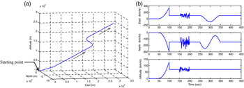
Figure 2. The scenario for simulation: (a) three dimensional trajectory of the vehicle and (b) the east, north, and altitude components of the vehicle velocity.
Table 3. Description of the vehicle motion.
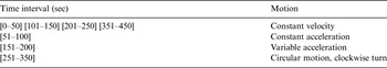
It is assumed that the Differential GPS (DGPS) mode is used, and most of the receiver-dependent errors are removed. We assume the remaining errors, mostly caused by multipath errors and thermal noise, follow a Gaussian mixture distribution of the form, defined by the PDF of the form
 $$f_{\bf X} (x) = \left( {\displaystyle{{1 - \varepsilon} \over {\sigma _1 \sqrt {2\pi}}}} \right)\exp \left[ { - \left( {\displaystyle{{x^2} \over {2\sigma _1^2}}} \right)} \right] + \left( {\displaystyle{\varepsilon \over {\sigma _2 \sqrt {2\pi}}}} \right)\exp \left[ { - \left( {\displaystyle{{x^2} \over {2\sigma _2^2}}} \right)} \right]$$
or equivalently by ${\bf X}\sim(1 - \varepsilon )N(0, \sigma _1^2 ) + \varepsilon N(0, \sigma _2^2 )$
, where σ
1 and σ
2 are the standard deviations of the individual Gaussian distributions, and ε is a perturbing parameter that represents error model contamination. In order to demonstrate the validity of the robustness of the proposed algorithm in non-Gaussian distributions, the perturbed conditions ε = 0·6 (i.e., with 60% contamination), and σ
2 = 10σ
1 = 10 × 1 (m) have been used. Figure 3 shows the Gaussian mixture model for the pseudorange errors in the simulation. The initial measurement noise variances
${\bf X}\sim(1 - \varepsilon )N(0, \sigma _1^2 ) + \varepsilon N(0, \sigma _2^2 )$
, where σ
1 and σ
2 are the standard deviations of the individual Gaussian distributions, and ε is a perturbing parameter that represents error model contamination. In order to demonstrate the validity of the robustness of the proposed algorithm in non-Gaussian distributions, the perturbed conditions ε = 0·6 (i.e., with 60% contamination), and σ
2 = 10σ
1 = 10 × 1 (m) have been used. Figure 3 shows the Gaussian mixture model for the pseudorange errors in the simulation. The initial measurement noise variances $r_{\rho _i} $
value are set to be 8 m2. The parameters utilised are α = 1·4, β = 2·5, κ = 0 in the UKF; γ = 1·345 in the CKF, for which the same value of the bounded-influence estimation selected by Huber (Reference Huber1981) is used.
$r_{\rho _i} $
value are set to be 8 m2. The parameters utilised are α = 1·4, β = 2·5, κ = 0 in the UKF; γ = 1·345 in the CKF, for which the same value of the bounded-influence estimation selected by Huber (Reference Huber1981) is used.
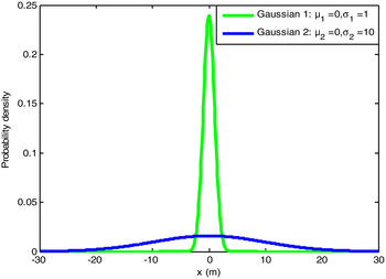
Figure 3. The Gaussian mixture model used in the simulation of pseudorange errors.
The results are shown in Figures 4–6. Prior to the incorporation of the Huber M-estimation mechanism, the GPS navigation accuracies based on the conventional nonlinear approaches: EKF, UKF and CKF are presented, shown in Figure 4, where the merits of the CKF have been shown. After that, evaluation of the results based on the nonlinear approaches compared to the Huber-based M-estimation CKF approach is conducted. Figure 5 provides comparison for the three types of filters: UKF, CKF, and HCKF. To show the benefit of the Huber M-estimation methodology, the comparison among Huber-based EKF, Huber-based UKF and Huber-based CKF has also be presented, shown in Figure 6. The HCKF, which inherits the virtue of robustness, shows the best performance among the various approaches. The simulation results show the superiority of the HCKF in highly dynamic situations which lead to the model to be mismatched to the actual situation. The improvement in robustness for the non-Gaussian measurement errors has also been presented.
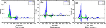
Figure 4. Comparison of positioning errors for EKF, UKF and CKF.
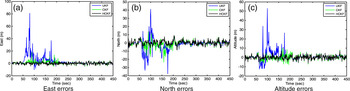
Figure 5. Comparison of positioning errors for UKF, CKF and HCKF.
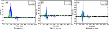
Figure 6. Comparison of positioning errors for HEKF, HUKF and HCKF.
Several important remarks are given as follows.
-
(1) In the four time intervals, 0–50, 101–150, 201–250, 350–450 s, the vehicle does not conduct manoeuvring and is performing constant-velocity straight-line motion. The navigation errors of all the nonlinear filters are not significantly distinguishable between the six methods.
-
(2) In the three time intervals, 51–100, 151–200, 251–350 s, the vehicle is conducting manoeuvring (constant acceleration, variable acceleration, or circular motion). The model mismatch to the actual situation leads to increased errors, as can be seen from the solution using the standard EKF. The CKF is about to converge in the high dynamic regions where there still exist noticeably large errors for the UKF-based solutions. However, performances based on the nonlinear filters are sensitive when the actual noise distribution deviates from the assumed Gaussian model. To further improve the performance of the CKF, a robust technique where the Huber M-estimation mechanism is incorporated can be utilised.
-
(3) When the GPS pseudorange observables are contaminated with non-Gaussian measurement errors, the CKF can adequately capture the non-Gaussianity and demonstrate noticeably better performance. Due to the appropriate tuning via the Huber M-estimation methodology, the HCKF exhibits robust behaviour and therefore outperforms the CKF when the non-Gaussian measurement errors are involved.
-
(4) The HCKF associates the contaminated measurements with an increase in the measurement covariance, causing the reformulated error covariance. This modified covariance inflation is known to cause an increase in the state estimation error due to the fact that all measurements are processed as if they were outliers.
-
(5) The HCKF and CKF filters give comparable results to each other for the positioning error during the non-manoeuvring intervals, while the HCKF provides a substantially improved performance in the high dynamic regions (51–100, 151–200, and 251–350 s), where it adequately captures both nonlinearity and non-Gaussianity. The HCKF is expected to provide further improved performance since the residual error covariance and measurement information used in computing the Huber M-estimation is the ML estimates for perfectly compensating against deviations from Gaussianity. The navigation results show that the HCKF demonstrates superior performance as compared to the other approaches.
4.3. Outdoor tests
Two tests conducted outdoors were carried out to further validate the effectiveness of the proposed algorithm. The two tests conducted at the National Taiwan Ocean University (NTOU) campus involved a field test and a rooftop experiment. The data collected by the Ashtech GPS receiver (DG14 module) was used for processing to perform a comparative study on navigation performance using various nonlinear estimators. The sampling rate of the measurements is 1 Hz. The measurement noise variances $r_{\rho _i} $
value are set to be 100 m2. The test results were obtained by post-processing of logged sensor data using the Matlab® software. The high accuracy relative positioning solution was used as the reference trajectory.
$r_{\rho _i} $
value are set to be 100 m2. The test results were obtained by post-processing of logged sensor data using the Matlab® software. The high accuracy relative positioning solution was used as the reference trajectory.
4.3.1. Field test
The first dataset was collected on the sports field at the university campus, shown in Figure 7. The raw data was collected for 140 seconds. In this test, the number of visible satellites varied between eight and nine in the clear open sky. To investigate the effect due to the contaminated non-Gaussian measurement errors, additional errors in the GPS pseudorange observables are added. The errors are assumed to possess the distribution again in the form as in Figure 3. Figure 8 shows the positioning errors for EKF, UKF and CKF. The CKF framework possesses some capability to deal with the non-Gaussian measurement errors/outliers. A comparison of the positioning errors for the three types of filters: UKF, CKF, and HCKF, is shown in Figure 9.
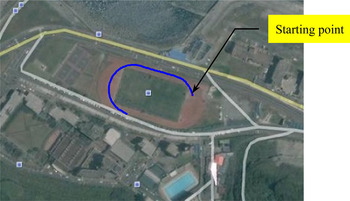
Figure 7. The trajectory for the field test in Google map.
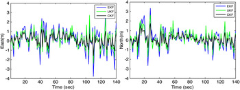
Figure 8. Positioning errors for EKF, UKF and CKF – the field test.
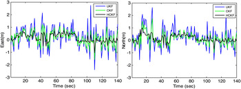
Figure 9. Positioning errors for UKF, CKF and HCKF– the field test.
4.3.2. Rooftop experiment
The second dataset selected for performance evaluation was collected on the rooftop of the department building. The trajectory for the rooftop experiment is shown in Figure 10, where a close look at the trajectory is also provided using the data collected by the Ashtech GPS receiver. The picture shown inside the trajectory based on the Ashtech GPS receiver is a zoomed-in shot for the upper right corner where a red tower is located. The starting point of the trajectory is at one side of the red tower, and the terminated point at the other side. In this experiment, the raw data was collected for 124 seconds. The rooftop environment presented a negative impact on the quality of GPS signals in such a challenging multipath environment. In this environment, there are several reflective objects on the rooftop, including the door that provides access to the roof. In addition, there are several other antennae in the vicinity. Multipath reflections from rooftop objects introduced a significant number of non-Gaussian errors to the GPS pseudorange observables. Furthermore, some of the GPS signals were blocked by the mountains in the south such that the number of visible satellites varied between four and seven, as shown in Figure 11. Figure 12 presents the positioning errors for the four approaches: EKF, UKF, CKF and HCKF.
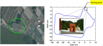
Figure 10. The trajectory for the rooftop experiment by Google map (left, circled area) and by the data collected by the Ashtech GPS receiver (right), respectively.
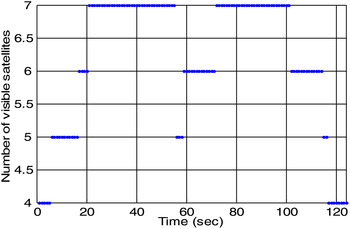
Figure 11. Number of visible satellites for the rooftop experiment.
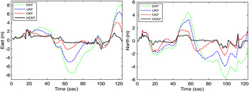
Figure 12. Positioning errors for EKF, UKF, CKF and HCKF–the rooftop experiment.
The results for the two outdoor tests do not try to demonstrate the superiority of the HCKF in high dynamic environments, but exhibit effectiveness against the non-Gaussian measurement errors. In the above three illustrative examples, the improvement due to the incorporation of the Huber M-estimation mechanism has been demonstrated. The GPS positioning errors clearly show the superiority of the HCKF algorithm.
5. CONCLUSIONS
This paper has presented a Huber-based Cubature Kalman Filter (HCKF) for GPS navigation processing. The measurements are GPS pseudorange observables contaminated with non-Gaussian errors. The cubature Kalman filter is based on the third-degree spherical-radial cubature rule to propagate the cubature points through the nonlinear functions, so as to solve the integration in the Bayesian filtering problem for numerically computing the multivariate moment integrals. The Huber M-estimation methodology is essentially based on Huber's generalised ML estimation theory, which exhibits robustness against the deviations from the Gaussian distribution.
The HCKF algorithm integrates the merits of the Huber M-estimation methodology to handle non-Gaussian errors or outliers and the cubature Kalman filter to avoid the numerical instability problem and improve the estimation accuracy in high-dimensional systems. The CKF framework was recast in the form of a sequence of nonlinear regression problems to be solved, at each measurement update using the robust Huber M-estimation methodology so as to enhance the CKF performance. In addition to the simulation test, the real GPS navigation data is also applied to validate the proposed algorithm. Performance comparisons on the six types of filters, EKF, UKF, CKF, HEKF, HUKF, and HCKF have been presented, among which the HCKF algorithm shows superior performance in GPS navigational accuracy.
ACKNOWLEDGMENT
This work has been supported in part by the Ministry of Science and Technology of the Republic of China under grant numbers NSC 101-2221-E-019-027-MY3 and MOST 104-2221-E-019-026-MY2.


