


1. Introduction
Multi-year seismic instrumentation of Antarctica has been historically sparse for regions not immediately accessible from the established science bases. This largely reflects the engineering and logistical challenges of year-round seismograph operation under extreme environmental conditions and limited opportunities for maintenance and data recovery. Scientific motivations (e.g. Podolskiy and Walter, Reference Podolskiy and Walter2016; Aster and Winberry, Reference Aster and Winberry2017) and instrumentation advancements over the last two decades have resulted in a dramatic increase in available seismic data, driven by numerous deployments of long-term or permanent broadband seismic instruments in both West and East Antarctica (Anthony and others, Reference Anthony2015).
In the last decade, two key developments in particular have removed the scientific and technical barriers to long-term, broadband ice shelf seismology. First, multiple studies utilizing local and teleseismic data from grounded-ice networks have established new analytical methods for stations sited on thick glacial ice (e.g. Barklage and others, Reference Barklage, Wiens, Nyblade and Anandakrishnan2009; Chaput and others, Reference Chaput2014) and the baseline models of seismic activity (Anthony and others, Reference Anthony2015, Reference Anthony, Aster and McGrath2017) necessary to contextualize broadband observations collected from an ice shelf-sited array. Second, community advancements in power and other technologies have produced lightweight broadband seismographs that are capable of continuous operation throughout multiple Antarctic winters.
Pioneering studies on ice shelf seismology have consisted of short-term deployments (<3 months) of single stations or small aperture arrays. High frequency experiments have focused on cryoseismic sources (Zhan and others, Reference Zhan, Tsai, Jackson and Helmberger2014) and active source imaging of ice shelf and seafloor structure (Kirchner and Bentley, Reference Kirchner and Bentley1979; Beaudoin and others, Reference Beaudoin, ten Brink and Stern1992). Other short-term studies placed broadband sensors at the Ross Ice Shelf (RIS) ice front and a free-floating iceberg and showed the viability of floating-ice-sited broadband seismometers as observatories of oceanic processes (Okal and MacAyeal, Reference Okal and MacAyeal2006; Cathles and others, Reference Cathles, Okal and MacAyeal2009), and even teleseismic earthquakes (MacAyeal and others, Reference MacAyeal, Okal, Aster and Bassis2009).
In late 2014, a 34-station broadband network (Fig. 1) was installed across the RIS for a 2-year study of oceanic, cryospheric and solid Earth processes (Bromirski and others, Reference Bromirski2015) by recording elastic and flexural-gravity waves on the ice shelf (Bromirski and Stephen, Reference Bromirski and Stephen2012). Ocean signals recorded atop large tabular floating ice bodies include tsunamis and infragravity waves (Bromirski and others, Reference Bromirski2017), ocean swell (Okal and MacAyeal, Reference Okal and MacAyeal2006; Cathles and others, Reference Cathles, Okal and MacAyeal2009; Baker and others, Reference Baker2019), waves from remote-calving events (MacAyeal and others, Reference MacAyeal, Okal, Aster and Bassis2009) and ice–ice and ice–seafloor interactions and their seismic and acoustic radiation (Talandier and others, Reference Talandier, Hyvernaud, Reymond and Okal2006; Dowdeswell and Bamber, Reference Dowdeswell and Bamber2007; MacAyeal and others, Reference MacAyeal, Okal, Aster and Bassis2008; Martin and others, Reference Martin2010). The RIS deployment additionally expanded opportunities for solid Earth studies in the sparsely-sampled Ross Embayment sector of the Antarctic plate; Shen and others (Reference Shen2018) applied ambient noise Rayleigh wave tomography to invert mantle S-wave velocity structure, and White-Gaynor and others (Reference White-Gaynor2019) applied teleseismic P-wave arrival time tomography to invert mantle P-wave velocity structure. Scientific motivations for this region include tectonic province boundaries, possible plumes (Seroussi and others, Reference Seroussi, Ivins, Wiens and Bondzio2017; Phillips and others, Reference Phillips2018) and the activity and origins of Antarctica's intraplate volcanism (e.g. Kyle and others, Reference Kyle, Moore and Thirlwall1992; Hole and LeMasurier, Reference Hole and LeMasurier1994; Reusch and others, Reference Reusch2008; Lough and others, Reference Lough2013). Heat flow, elastic lithosphere thickness and mantle viscosity constrained by geodesy and seismic proxies (Ramirez and others, Reference Ramirez2016; O'Donnell and others, Reference O'Donnell2017) have important implications for West Antarctic Ice Sheet dynamics and stability (Rignot and Jacobs, Reference Rignot and Jacobs2002; Joughin and Alley, Reference Joughin and Alley2011; Barletta and others, Reference Barletta2018).
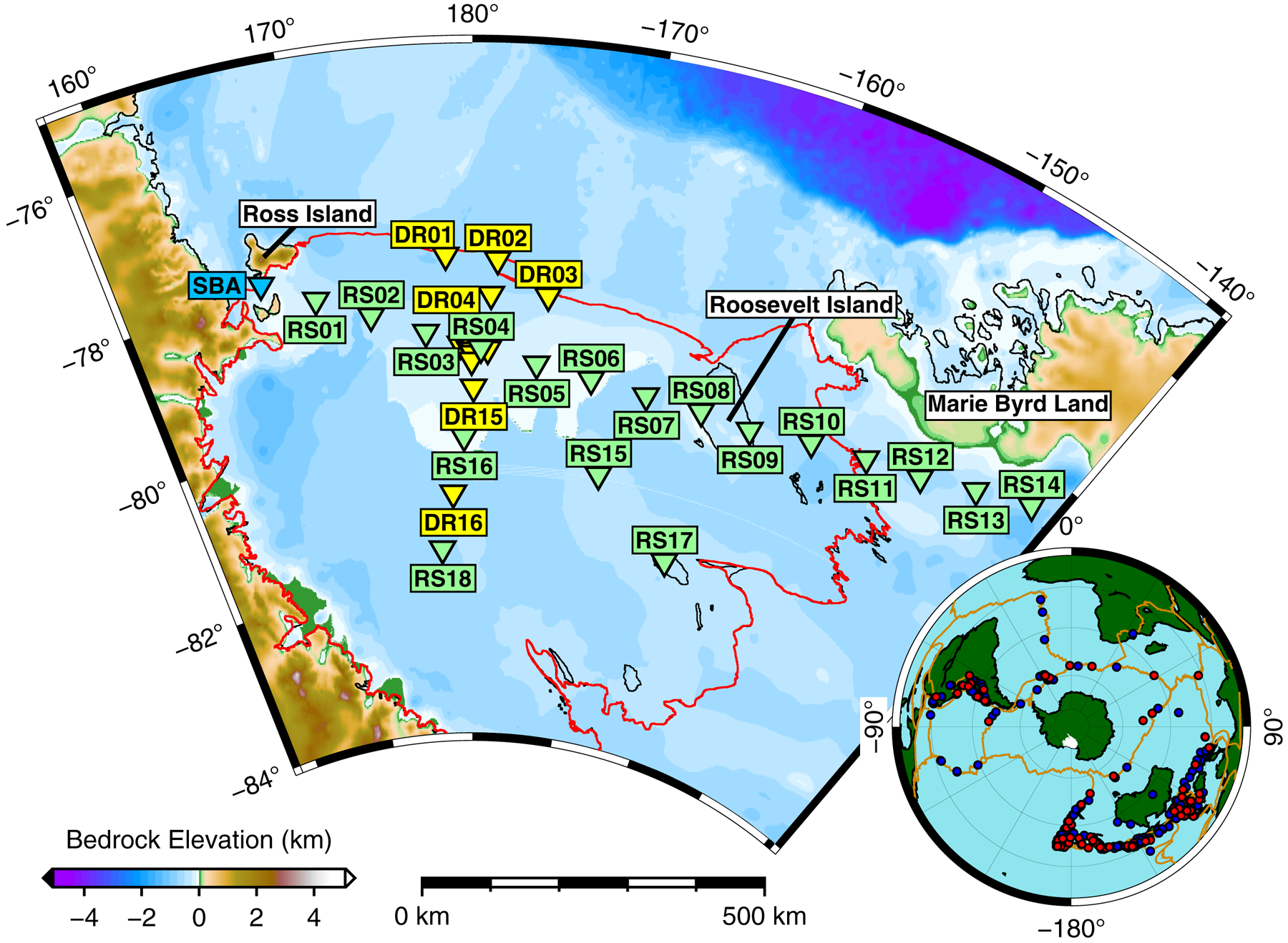
Fig. 1. RIS/DRIS array station locations. DR stations not explicitly labeled here (DR05–DR14; unlabeled yellow triangles) were deployed in the vicinity of central station RS04 (Fig. S1). All RS and DR stations were deployed on ice and all were on the floating ice shelf with the exception of: RS08 and RS09 on Roosevelt Island RS11–RS14 on the West Antarctic Ice Sheet in Marie Byrd Land; and RS17 on Steershead Ice Rise. Global Seismographic Network station SBA on Ross Island (blue) is also shown. The RIS is outlined in red. Inset: Map of summer (red) and winter (blue) earthquakes used in this study. Antarctica is displayed with the traditional Grid-North orientation. Tectonic plate boundaries are shown in orange (Bird, Reference Bird2003).
The ambient seismic environment of the RIS has been previously documented at short periods (<1 s) by Diez and others (Reference Diez2016) and Chaput and others (Reference Chaput2018), and for longer periods (>30 s) by MacAyeal and others (Reference MacAyeal2006), Cathles and others (Reference Cathles, Okal and MacAyeal2009), Bromirski and others (Reference Bromirski2017) and Chen and others (Reference Chen2018). For intermediate periods (0.5–20 s), Baker and others (Reference Baker2019) present seasonal and geographic variations in the RIS noise field and discuss potential source mechanisms. Our current signal-noise analysis makes extensive use of Baker and others (Reference Baker2019) and may be viewed as a companion piece to that work.
We present a signal-to-noise analysis of teleseismic P-wave (0.5–2.0 s period), S-wave (10–15 s) and surface wave (17–23 s) arrivals and their immediate coda. We show that these signals may be readily observed at floating-ice-sited seismographs, but are strongly modulated by seasonal changes in ocean wave-generated noise. We quantify how teleseismic observations are affected by station proximity to the RIS ice front and grounding zones and note secondary wavefields that are excited within the RIS by teleseismic wavefields. We utilize acoustic and Crary (i.e. SV-waves trapped in floating ice) resonances to estimate water column and ice thicknesses, respectively. We interpret observations of teleseismic arrivals at floating stations to be consistent with a theoretical ‘acoustic cutoff’ period delimiting compressible and incompressible regimes within the water column. We document the common conversion of teleseismic S-wave energy at grounding zones into fundamental mode, symmetric (S0) Lamb waves (e.g. Fig. 2) which may propagate 250 km or more into the ice shelf interior; to our knowledge, this phenomena has not been previously described. Finally, we document teleseismic surface wave dispersion on the ice shelf and present representative group velocity curves for Rayleigh waves.

Fig. 2. Schematic of the secondary wavefields generated within a floating plate by teleseismic body wave arrivals (‘P-wave’ and ‘SV-wave’). ‘Crary Resonance’ refers to an SV-wave resonance within the ice layer; this resonance may occur at non-critical angles for the ice/water layer interface and is therefore akin to a leaky Crary wave. An ‘Acoustic Resonance’ is simply P-waves reverberating within the water column. ‘S0 Lamb Wave’ shows the fundamental-mode symmetric Lamb wave generated by a teleseismic SV-wave incident at the grounding zone, with SV particle displacement perpendicular to the grounding line. Other plate modes are possible (e.g. P-to-SV resonances within the ice, or shear horizontal plate waves generated by SH-waves incident at the grounding zone) but are not illustrated here.
2. Data and methods
2.1. Instrumentation
The coordinated RIS (Mantle Structure and Dynamics of the Ross Sea from a Passive Seismic Deployment on the Ross Ice Shelf) and DRIS (Dynamic Response of the Ross Ice Shelf to Wave-Induced Vibrations) projects (Figs 1, S1) consisted of 34 polar-engineered broadband seismic stations provided by the Incorporated Research Institutions for Seismology (IRIS) Polar Programs. The RIS/DRIS stations were installed in late 2014 and recorded ~2 years of continuous data. Seismographs were deployed in two main transects: a 1100 km-long ice-front-parallel transect (W–E) and a 425 km long ice-front-perpendicular transect (N–S). The network consisted of (1) a shelf-spanning large aperture array (RS01–RS18) with a median spacing of 83 km and (2) a central medium aperture array (DR01–DR16) with stations spaced at 20–50 km. RS04 is located at the intersection of the two main transects. All stations were sited on floating ice, with the exceptions of RS08 and RS09 on Roosevelt Island, RS11–RS14 in Marie Byrd Land and RS17 on Steershead Ice Rise. .
Most RIS (RS) and DRIS (DR) stations utilized Nanometrics Trillium 120PH posthole sensors direct-buried at depths of 2–3 m below the snow surface; exceptions were RS09, RS11–RS14 and RS17, which were Nanometrics Trillium 120PA sensors installed on phenolic resin pads within shallow vaults. All DR stations and RS04 had a sampling rate of 200 Hz; all other RS stations had a sampling rate of 100 Hz. Stations used solar power during the Antarctic summer and single-use lithium thionyl batteries during the winter. Due to Iridium satellite modem power and bandwidth constraints, only state-of-health information was telemetered, and the network was therefore serviced in 2015 for intermediate data recovery and any other necessary servicing. The signal-to-noise analysis presented here incorporates data from the full deployment period of approximately November 2014 through November 2016. Stations RS10–RS14 remained deployed in Marie Byrd Land until early February 2017 due to logistical issues.
2.2. Teleseismic earthquake signals on the RIS
We perform a signal-to-noise ratio (SNR) analysis for teleseismic earthquake signals (M w 5.5 or greater) observed by the RIS/DRIS stations at epicentral distances >30°, selecting P-wave, S-wave and surface wave arrivals and their immediate coda, with spectral bandpass filtering and signal times shown in Table 1. The epicentral distribution and the Gutenberg–Richter relation for all events are shown in Figure S2. Predicted arrival times for individual phases for all earthquakes are based on ak135 travel time curves (Kennett and others, Reference Kennett, Engdahl and Buland1995). Bandpass filtering was determined based on the peak periods of the median modified SNR curves.
Table 1. Parameters for teleseismic signals used in this study
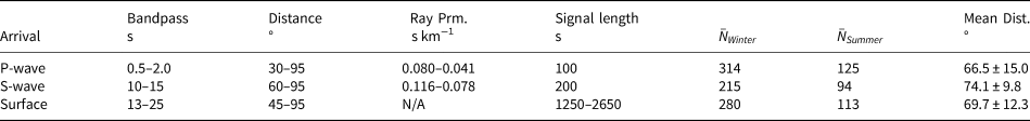
$\bar {N}$ indicates the mean number of events across all stations for each season. Summer includes all events between 1 December and 31 March. Winter includes all events between 1 April and 30 November. P- and S-wave signal lengths were chosen based on a survey of observed coda durations and to avoid contamination by subsequent phases. ‘Mean Dist.’ indicates the mean arc distance and standard deviation across all stations and all events. The mean magnitude for all bands, across all stations and all events, was M w = 6.0 ± 0.5.
To characterize teleseismic P-wave signals, we examine events at epicentral distances between 30° (slowness 0.08 s km−1) and 95° (0.04 s km−1) from each station. The teleseismic S-wave catalog is limited to events between 60° and 95° to prevent interference from surface wave arrivals near 5 km s−1. Teleseismic P- and S-wave arrivals are separated by a minimum of ~300 s (at 30°) and therefore will not mutually interfere. The surface wave analysis uses wavetrains in the 4 to 2 km s−1 arrival window, from earthquakes with epicentral distances between 45° and 100°, to prevent interference from body waves.
The ambient noise field of the RIS in the 0.4–30 s period band has seasonal variations of ~5–20 dB (Baker and others, Reference Baker2019). This variation is bimodal between the austral summer and winter and reflects the attenuation of wind-sea and ocean gravity waves in the Ross Sea by the formation of spatially continuous sea ice during the winter months. The absence of extensive, continuous sea ice determines the onset and termination dates of the ‘summer’ high-noise state analyzed in Baker and others (Reference Baker2019). We similarly subdivide our catalog into ‘summer’ earthquakes occurring during the approximate open-water interval between 1 December and 31 March, and ‘winter’ earthquakes occurring during the remainder of the year during which sea ice is broadly contiguous at the ice shelf front. Note that we henceforth refer to ‘winter’ and ‘summer’ noise conditions as indicating these annual sea ice-determined time periods, consistent with Baker and others (Reference Baker2019), and not the formal austral seasons.
2.3. Spectral characterization of teleseismic signals
The SNR ratios of individual events generally depend on a variety of source and propagation factors (e.g. moment, radiation pattern, depth, distance and mantle heterogeneities) which must be minimized to ensure that any observed temporospatial variations are solely the result of receiver-side features. We use event stacking and source normalization (described below) to approximate a globally-averaged teleseismic wavefield for comparison to station-specific noise fields. Additionally, we focus on the teleseismic excitation of the ice shelf beyond that of initial phase arrivals (in contrast to White-Gaynor and others (Reference White-Gaynor2019)).
For body wave arrivals, the phase arrival and its subsequent coda are extracted in fixed duration time segments (Table 1) regardless of epicentral distance, back azimuth and magnitude. S-wave signals with epicentral distances >~82° are referenced to the SKS phase. For surface wave trains, we analyze 4–2 km s−1 surface waves, with a total signal length that is dependent on epicentral distance. Data segments for all three arrival types include 10 s of pre-arrival noise as a buffer against potential deviations from predicted arrival times and to allow tapering of processing artifacts without attenuation of the actual signal. For all segment types, the ‘noise’ time series is drawn from immediate pre-arrival data using an equal number of seconds as the ‘signal’ analysis. For example, for a P-wave arriving at t 0 = 0 s, the noise data are comprised of T n = [t 0 − 110…t 0] s, while the signal data spans T s = [t 0 − 10…t 0 + 100] s. All data are de-meaned, de-trended, cosine-tapered by 5 s, decimated to 10 Hz, and rotated to (Z, R, T) (vertical, radial, transverse) coordinates using USGS NEIC Comcat parameters.
SNR spectra are calculated as the ratios of the signal and noise power spectral densities (PSD). PSDs are estimated using Welch's method (Welch, Reference Welch1967), with the number of (Hann-tapered) sub-segments determined by requiring 80% overlap and sub-segment lengths approximately equal to ten times the upper period limits indicated in Table 1. PSD estimates are subsequently smoothed by averaging over 1/8 octave bins in 1/16 octave increments.
Due to the geographic extent of the RIS/DRIS array and the nonuniform distribution of earthquake sources (Fig. 1), not all stations observed the same population of earthquakes given the event selection criteria. These disparities are especially exaggerated during our defined high-noise, low-sea-ice summer months (1 December–31 March), which include roughly a quarter of the number of events as the winter months (1 April–30 November). For the goals of this study, we require an idealized teleseismic source that is uniformly observed by all stations, such that interstation variations in SNR are predominantly controlled by receiver-side phenomena. To approximate such a source, we apply a correction analogous to the relative radiometric normalization used in remote sensing, but operating on the source rather than the receiver. We normalize individual earthquake SNRs to a theoretical earthquake model, with a scaling factor based on USGS seismic moment and losses from geometric spreading. For P- and S-waves, the corrected SNR′ is:

where SNR is the uncorrected signal-to-noise ratio, M 0 and M 0ref are the event and reference seismic moments, respectively and D and D ref are the depth-dependent, source-to-receiver ray path distances through a spherical ak135 Earth model. For surface waves, the correction is:

where Δ and Δref are the great arc distances, and the sine function corrects for two-dimensional spreading (Stein and Wysession, Reference Stein and Wysession2009). We use a reference event with a magnitude of M w = 6.0 (the approximate mean of all observed events), band-specific great arc distances as listed in Table 1, and a depth of 10 km.
We make no attempt to correct for source function beyond median stacking, nor do we eliminate overlapping events. For our S-wave analysis, the strength of the P-wave coda integrated into the S-wave noise estimate may be dependent on epicentral distance if the P-wave coda decays appreciably within the noise window. That is, S-wave noise estimates for more distant earthquakes may integrate a smaller percentage of the P-wave coda than those for less distant earthquakes. Based on our generally symmetric earthquake catalog (Figs 1, S2), we expect that median stacking will neutralize any spatial biasing relative to the receiver-side spatial variations. Surface wave noise estimates incorporate the entirely of the associated P- and S-wave codas regardless of epicentral distance and are therefore insensitive to this issue.
To evaluate seasonal variations in SNR, we calculate the seasonal median SNR from all appropriate summer and winter events, as defined above and by Baker and others (Reference Baker2019). We evaluate spatial variations across the RIS/DRIS array with respect to the mean of station-specific median seasonal PSDs for the arrival bandpass ranges listed in Table 1.
3. Elastic waves in an ice shelf
Floating tabular ice bodies support elastic-gravity wavefields that are generally not encountered elsewhere in seismology (e.g. Viktorov, Reference Viktorov1967; Sergienko, Reference Sergienko2017; Chen and others, Reference Chen2018; Baker and others, Reference Baker2019). Here, we provide an overview of the short-to-intermediate period (<20 s) wave phenomena for floating elastic plates that are relevant to this study.
3.1. Elastic structure
The RIS spans an area of 487, 000 km2 and floats on the relatively shallow continental shelf waters of the Ross Sea embayment with only sparse internal pinning points. RIS/DRIS station sites have ice thicknesses of 200–400 m (median 325 m; $\widetilde {h}$ ) and water column thicknesses of 100–700 m (median 464 m; $\widetilde {H}$
 ) in BEDMAP2 (Fretwell and others, Reference Fretwell2013).
Laterally varying structures in ice shelves are introduced by the convergence of source glaciers near the grounding line and by the subsequent advection of shelf ice toward the RIS calving front, at up to 1 km a−1 for the RIS (Mouginot and others, Reference Mouginot, Rignot and Scheuchl2019). Internal structures include suture zones between tributary glaciers that persist to the terminus of the RIS ice front. Also present are subglacial and surface crevasses and rifts that are generally parallel with the calving front, reflecting a broadly tensional stress state in the seaward flow direction. This tensional stress field is magnified near the free-floating terminus (LeDoux and others, Reference LeDoux, Hulbe, Forbes, Scambos and Alley2017) and is cyclically influenced by tidal tilt (e.g. Olinger and others, Reference Olinger2019). Significant vertical structure includes a meteoritic snow-firn layer that transitions to glacial ice over tens of meters (e.g. Diez and others, Reference Diez2016), and for some shelves, a seasonally modulated basal freeze layer. The sub-shelf seafloor may be comprised of up to several kilometers of low velocity lithified sediment overlying a high velocity basement (e.g. Beaudoin and others, Reference Beaudoin, ten Brink and Stern1992).
We assume bulk elastic properties for the RIS system as listed in Table 2. We also assume that the RIS is laterally and vertically homogeneous and isotropic, with ice/water and water/seafloor interfaces that vary smoothly at scales much longer than the ice thickness. We justify this simplification by noting that the RIS/DRIS stations were deliberately sited in regions of solid glacial ice several kilometers or more distant from crevassed or rifted areas as a matter of safety. For teleseismic body wave arrivals (i.e. Table 1) with near-normal angles of incidence, the maximum ice shelf basal piercing distance would be 230 m for a P-wave with a ray parameter of 0.08 s km−1, assuming a 700 m thick shelf with a P-wave velocity of 3.87 km s−1. For vertical features, our simplification is justified by the resolution limit of the teleseismic waves of interest. Assuming a quarter-wavelength limit, the highest resolving wave would be an SV-wave generated by a teleseismic P-wave at the ice/water interface, with a period of 0.5 s and a seismic velocity of 2.0 km s−1, and a minimum resolution of 250 m. For contrast, the low-velocity firn layer becomes important only in the uppermost 60 m (Kirchner and Bentley, Reference Kirchner and Bentley1979; Beaudoin and others, Reference Beaudoin, ten Brink and Stern1992; Diez and others, Reference Diez2016).
Table 2. Elastic parameters for the RIS used in this study
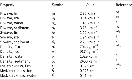
Firn values are the geometric mean of empirical results published in the listed references.
aKirchner and Bentley (Reference Kirchner and Bentley1979).
bFofonoff and Millard (Reference Fofonoff and Millard1983).
cBeaudoin and others (Reference Beaudoin, ten Brink and Stern1992).
dKing and Jarvis (Reference King and Jarvis2007).
eGriggs and Bamber (Reference Griggs and Bamber2011).
fFretwell and others (Reference Fretwell2013).
gDiez and others (Reference Diez2016).
3.2. Intralayer resonances
High seismic impedance contrasts in the vertical structure of an ice shelf system – specifically at the ice/water, water/seafloor and sediment/basement interfaces – create strong reverberatory wavefields by multiply reflecting incident body waves. A similar but less severe effect is common in geologic basins, where low velocity sediment overlies high velocity basement rock. The amplitude of this effect is maximized when the wavefield constructively interferes with itself. For any individual layer, the resonance periods, P R are:

where Z is the layer thickness, η is the vertical slowness of the incident primary wavefield, the integers n are harmonic mode orders and m accounts for phase reversals at reflective interfaces (modified from Press and Ewing, Reference Press and Ewing1951; Crary, Reference Crary1954). For resonances spanning multiple layers, the period is simply the series summation of all layers. For the ice shelf system, strong resonance wavefields may be generated for S-waves within the ice shelf and P-waves within the water column.
The layered structure of an ice shelf creates a highly efficient waveguide for plane-media polarizations of shear waves. SH-waves within an ideal ice shelf with perfectly horizontal boundaries undergo lossless, in-phase reflections (m = 0) at the free surface and the ice/water interface; at any resonance period, P R, an SH-polarized shear wavefield will propagate laterally along the ice shelf as a shear horizontal plate wave (Press and Ewing, Reference Press and Ewing1951; Rose, Reference Rose1999). SV-waves will experience lossless, out-of-phase reflections (m = 1) from either boundary only at the critical angle $\theta _{\rm c} = \sin ^{-1}\lpar \beta _{\rm i} \alpha _{\rm i}^{-1}\rpar$ ; a critically reflected SV-wavefield (m = 1) at any P R will propagate laterally along the ice shelf as a Crary wave (Crary, Reference Crary1954). SV-waves incident on the ice/water interface at all angles other than θ c will lose energy via SV-to-P conversions within the ice and water (Fig. S3).
For the structure specified in Table 2, θ c = 29.6°, equivalent to a ray parameter of p = 0.263 s km−1. Therefore, we do not expect to observe excitation of Crary waves by teleseismic body waves, for which p = 0.04–0.12 s km −1. However, the steeply incident ray parameters typical of teleseismic P-waves result in non-negligible P-to-SV conversion coefficients (10–20%) for both the free surface and the ice/water interface, with strong SV reflection coefficients (>80%), and no phase shift (m = 0) (Fig. S3). Furthermore, for the ice shelf values listed in Table 2, and a ray parameter of p = 0.06 s km−1, Eqn (3) yields P R = 0.33 s, which is generally within the spectral content of the P-wave teleseismic signal. We therefore expect to observe significant SV-resonant energy associated with these arrivals. We will refer to these as Crary resonances to differentiate them from true, lossless Crary waves.
SH-wave energy may potentially be observed coincident with teleseismic P-wave arrivals as a result of scattering from sloping interfaces or due to ice anisotropy. We do not expect to observe Crary resonances associated with teleseismic S-waves, due in part to their longer periods being incompatible with the RIS resonant periods, and for additional reasons to be discussed later in this section.
Extending the previous resonance analysis to the water column, we expect teleseismic P-wave codas to excite acoustic resonances (m = 0) with periods near P R = 0.61 s. This resonance is markedly less efficient than the Crary resonance and will leak P- and SV-wave energy into the ice and seafloor. In Section 4.1 we show that the spectral signatures of these Crary and acoustic resonances may be exploited to accurately estimate the thicknesses of the RIS and the sub-shelf water column.
3.3. Coupling of seismic, acoustic and gravity waves
For elastic waves within an open water column of finite depth H (i.e. bounded by a free surface and a solid elastic Earth), there exists an acoustic cutoff period, $P_{\rm c} = 4H \alpha _{\rm w}^{-1}$ , above which any vertical component of displacement ceases to propagate and becomes evanescent (i.e. decays exponentially in the vertical direction) (Ewing and others, Reference Ewing, Jardetzky and Press1957). For oscillations at periods greater than P c, gravity becomes increasingly relevant to the vertical restoring force, and completely dominates for periods greater than the Brunt-Väisälä period (Apel, Reference Apel1987). For the period band bounded by the acoustic cutoff period and the Brunt-Väisälä period, the propagation of oscillatory energy through the water column lies in the acoustic-gravity wave domain. Traer and Gerstoft (Reference Traer and Gerstoft2014) and Ardhuin and Herbers (Reference Ardhuin and Herbers2013) provide derivations of this wave type as an extension of the nonlinear wave–wave interaction model first proposed by Hasselmann (Reference Hasselmann1966). From the perspective of continuum mechanics, this acoustic-gravity regime may be understood as a transition between compressible and incompressible fluid behavior with increasing period. Useful analytical representations for the response of an ocean above vertically displaced ocean floor are given by Yamamoto (Reference Yamamoto1982). Literature on acoustic-gravity waves is extensive but has focused on wave mechanics confined to the water layer. Recent studies have begun to address acoustic-gravity waves in the presence of an ice layer, but have thus far been restricted to inelastic ice caps (Kadri, Reference Kadri2016) or thin (h ≪ H) elastic sea ice (Abdolali and others, Reference Abdolali, Kadri, Parsons and Kirby2018) and thus do not address coupling between acoustic-gravity and seismic waves.
To obtain an estimate for the cutoff period for the combined ice shelf and water column at the RIS, we use the derivation for the similar case of a three-layered liquid half space (Ewing and others, Reference Ewing, Jardetzky and Press1957). We justify this simplification by noting that teleseismic P-waves propagate within the water column at an angle of incidence of 3.3–6.6° (0.04–0.08 s km−1) and therefore lose <5% energy at any interface via conversion to SV-waves (Figs S3, S4). This approximation does not account for the flexural rigidity of the ice shelf nor the overlying firn layer. The cutoff period, P c, in this case may be determined using:

where m i,w,s are vertical wave numbers within the ice, water and sediment layers, respectively, and δ 1 = ρ i/ρ w, δ 2 = ρ w/ρ s (Ewing and others, Reference Ewing, Jardetzky and Press1957). For the values listed in Table 2, P c ≈ 2.25 s and varies within ±0.6 s for the range of sub-station ice and water layer thicknesses.
Short-period teleseismic arrivals associated with the P-wave coda (0.5–2.0 s) are therefore predicted to be observable on all three channels at floating stations. However, longer-period (e.g. 10–15 s) teleseismic compressional energy (e.g. S-to-P converted phases originating at the sediment/basement interface) should be observable solely on the vertical channel, reflecting the water column's predominately incompressible response to longer-period vertical seafloor displacement (e.g. Ewing and others, Reference Ewing, Jardetzky and Press1957). Observations of Rayleigh waves (>15 s) are similarly expected to be vertically dominant (as previously noted by Okal and MacAyeal (Reference Okal and MacAyeal2006)). Love wave arrivals should not be observable by floating stations above a planar seafloor due to the zero traction horizontal boundary condition.
3.4. Coupling of seismic and plate waves
A floating ice layer is an elastic plate system and therefore supports a variety of elastic modes that are not observed in solid-Earth or ocean-bottom seismology. On an ice shelf, plate modes are expected to be excited by tractions imposed upon the ice by ocean gravity waves at the ice front and within the sub-shelf water cavity. At ultra-long periods (>3 h), ocean waves may generate normal modes across the entirety of the RIS, which may, in turn, couple into acoustic-gravity waves within the atmosphere (Godin and Zabotin, Reference Godin and Zabotin2016). At periods of 50–100 s, infragravity and tsunami waves originating up to thousands of kilometers away generate flexural-gravity waves (i.e. buoyancy-coupled asymmetric mode (A0) Lamb waves) which propagate several hundred kilometers into the RIS interior (Bromirski and others, Reference Bromirski2017). In the 1–50 s period band, ocean swell impacts at the ice front generate zeroth-order, symmetric mode (S0) Lamb waves, in addition to flexural-gravity modes (Chen and others, Reference Chen2018; Aster and others, Reference Aster2019). On the RIS, flexural-gravity wave motion dominates the ambient wavefield at distances <120 km from the ice front. At greater distances, extensional wave motion (i.e. S0 Lamb) dominates and is observable at least 450 km from the ice front (Chen and others, Reference Chen2018; Baker and others, Reference Baker2019).
Of interest to the present study are the symmetric mode Lamb waves (Lamb, Reference Lamb1917). Particle motion for these waves is retrograde elliptical in the vertical/radial plane, with a high eccentricity oriented parallel to the radial axis (Fig. 2). Lamb waves may be generated within a plate by compressional forces applied normal to the plate end face, or by shear forces applied in traction parallel to the basal plate surface. The theory and application of these methods have been rigorously documented in a number of publications on ultrasonics, where Lamb waves are often used in nondestructive testing (e.g. Viktorov, Reference Viktorov1967; Rose, Reference Rose1999). For this study, we concern ourselves with Lamb wave generation via normal end face tractions, such that:

where E L is the energy of the resulting Lamb wave, A is the amplitude of the source signal and ϕ is the angle between the source traction and the normal to the plate face (Rose, Reference Rose1999). For simplicity, we have restricted the source signal to oscillating within the same plane as the plate surface (i.e. horizontal). For the generation of ocean-coupled Lamb waves, the RIS is oriented such that ocean gravity waves propagating across the Ross Sea generally impact the ice shelf face at oblique-to-normal angles of incidence, maximizing the transfer of horizontal impulse between the incoming waves and the shelf.
The grounding lines of ice shelves are also plate boundaries at which Lamb wave energy may be generated. A relevant situation for this study is the case of teleseismic S-waves arriving near the grounding lines at nearly vertical angles of incidence (Fig. 2). Both SV- and SH-waves have the potential to generate Lamb wave energy (E L) according to the general relationships:

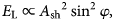

where A sv and A sh are the amplitudes of the SV- and SH-waves, respectively, θ gl is the strike of the grounding line (with the RIS defined as down-dip using the right-hand-rule convention) and θ eq is the back azimuth to the source earthquake.
4. Results
Figure 3 shows representative component spectrograms for an M w 6.4 earthquake recorded by floating station RS16. This spectrogram shows multiple features that are relevant to our discussion of the various arrival bands. Spectrograms for the same event recorded at grounded station RS08 are shown in Figure 4.
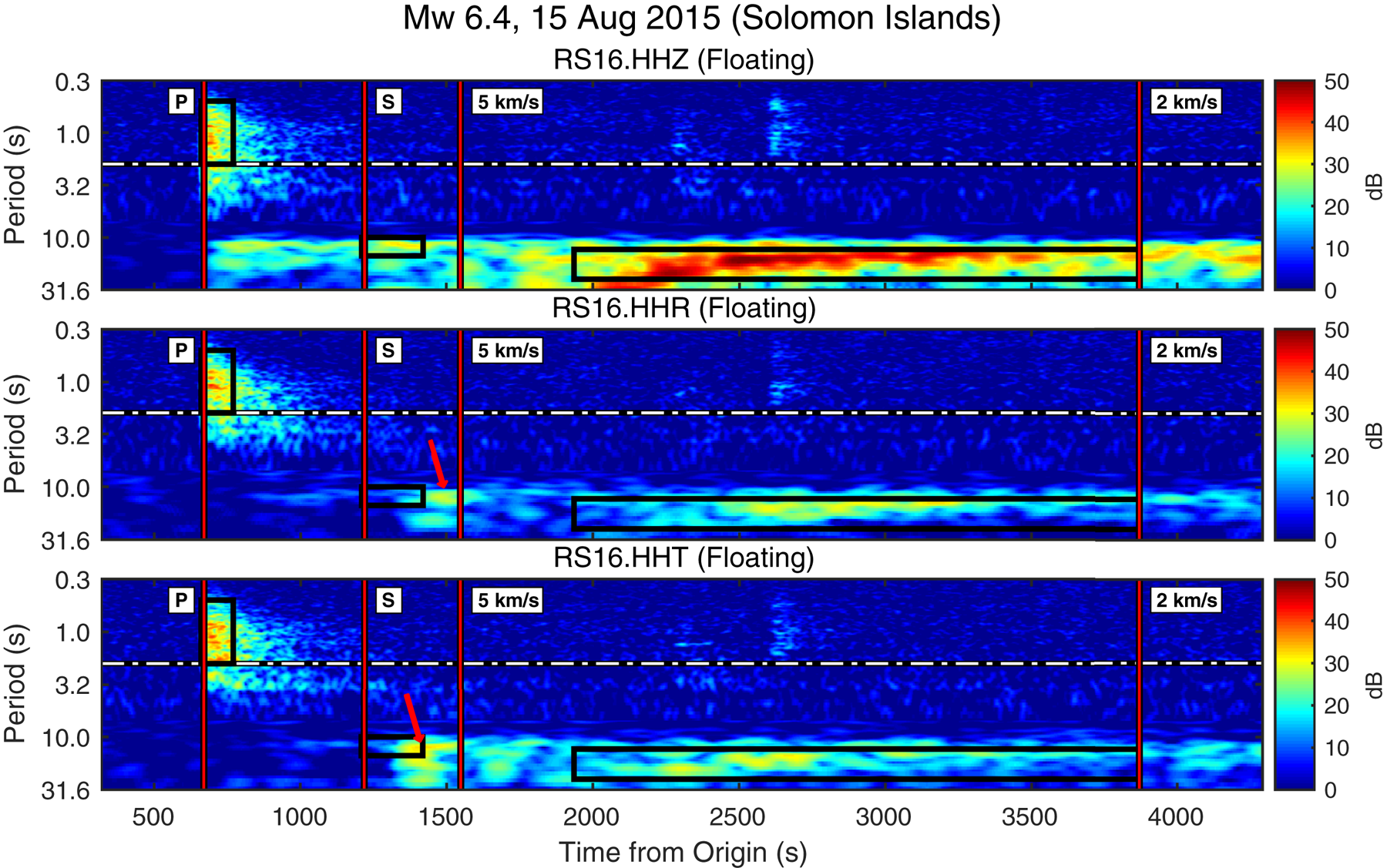
Fig. 3. Pre-P background-normalized spectrogram from floating station RS16 of an M w 6.4 earthquake east of the Solomon Islands, with an epicentral distance of 7740 km, a hypocenter depth of 8 km, and a back-azimuth of 345°. For periods <7.0 s, PSDs were calculated using 50 s segments in 0.5 s moving increments. For periods >7.0 s, PSDs were calculated for 200 s intervals in 2.0 s moving increments. Red vertical lines mark ak135-predicted arrival times. Black rectangles mark the spectral and temporal integration bounds used for signal analysis. White and black line marks the acoustic cutoff period as estimated using Eqn (4). Red arrows indicate probable Lamb waves generated by S-wave arrivals at RIS grounding lines to the southeast (HHR, Eqn (6)) and to the southwest (HHT, Eqn (7)). This event was recorded during winter low-noise conditions when continuous sea ice in the Ross Sea strongly attenuates ocean gravity waves before they can excite the RIS (Baker and others, Reference Baker2019) or generate strong microseisms (Anthony and others, Reference Anthony2015). Figure S5 shows the unnormalized spectrogram.
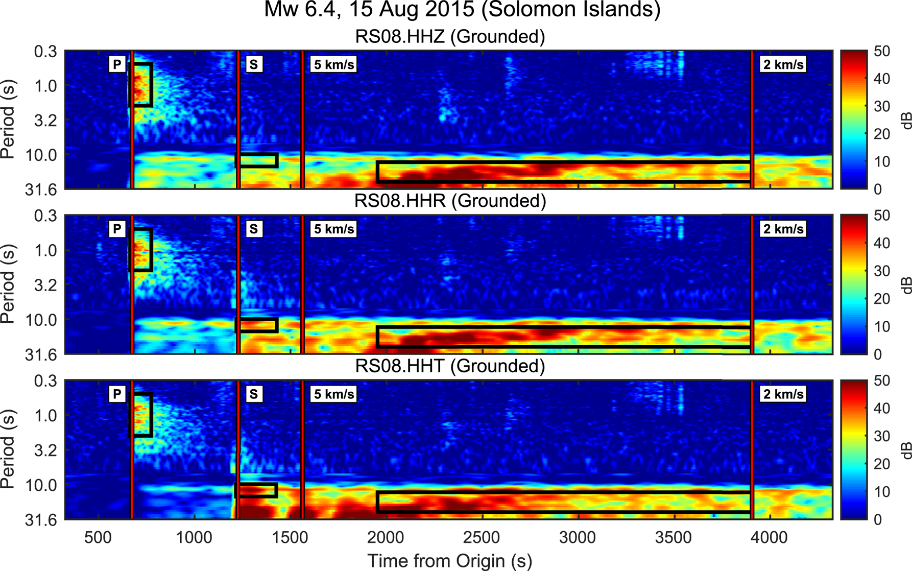
Fig. 4. Pre-P background-normalized spectrogram from grounded station RS08 for the same earthquake presented in Figure 3. Epicentral distance was 7800 km with a back-azimuth of 325°. Figure S6 shows the unnormalized spectrogram.
4.1. P-waves (0.5–2.0 s)
Teleseismic P-wave wavetrains in the 0.5–2.0 s period band are generally well-observed on the vertical and horizontal components of floating stations during both winter and summer noise conditions. In the 5–10 s band, secondary microseism noise overwhelms both vertical and horizontal component signal (Fig. S5). Notably, teleseism energy in the 10–20 s band is well-observed on the vertical component, but is very poorly observed on the horizontal components; for example, compare Figures 3 and 4. This relative lack of horizontal signal may reflect the transition of the water column from compressible to incompressible beyond the acoustic cutoff period (Eqn (4)); this behavior is addressed in detail in the Supplementary material.
Figure 5 shows spatial and seasonal variations in the mean SNR for teleseismic P-wave arrivals in the 0.5–2.0 s period band. During the winter low-noise state, mean vertical component SNR at nearly all floating ice stations for the P-wave and its immediate coda was ~25 dB, similar to the grounded ice stations on Roosevelt Island and in Marie Byrd Land (Fig. 5a, HHZ). Winter vertical SNR did not appear to be significantly affected by ice or water layer thicknesses nor by distance from the ice front (Figs 5a, b, respectively). The notable exceptions were the ice front stations (DR01–DR03), for which the vertical SNR dropped to 20 dB. The radial (HHR) and transverse (HHT) component SNRs showed greater spatial variations; along the W–E transect, SNR generally increased from 19 dB at RS01 to 23 dB at RS07, suggesting a possible dependence on increasing ice or decreasing water layer thicknesses. Along the N–S transect, horizontal SNR increased from 5 dB at DR02 to 23 dB for all stations farther than 120 km from the ice front. Surprisingly, the radial and transverse components show approximately equivalent SNR at most floating stations, except for those with the thickest ice and thinnest water columns (RS05–RS07), or those farthest from the ice front (DR16 and RS18). At these exceptional floating stations, and also all grounded stations, the radial SNRs were 2–3 dB higher than the transverse.
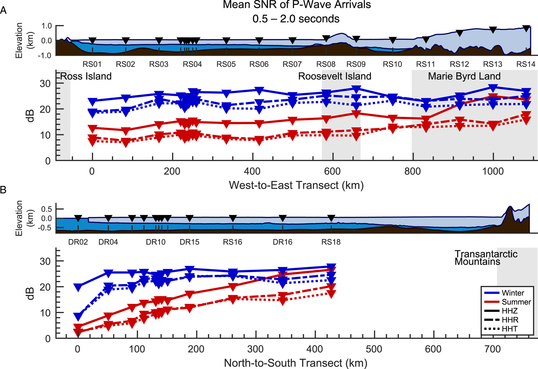
Fig. 5. Seasonal and geographic variations in average acceleration power for teleseismic P-wave arrivals, for the indicated seasonal SNR-PSD medians. Ice and water thickness profiles are based on BedMachine data. BedMachine uses an outdated coastline mask that excludes the current northward extent of the RIS; the RIS ice front currently sits ~3 km north of DR02. Gray backgrounds indicate approximate areas of grounded ice. Data have been corrected using Eqn (1); Figure S7 plots the uncorrected data.
The summer high-noise state predictably resulted in generally lower P-wave SNR at all stations. Along the W–E transect, SNR dropped by 8–12 dB across all three components for all floating stations and the grounded stations closest to the grounding zones (RS08, RS09 and RS11; Fig. 5a). Stations RS12–RS14, located more than 110 km inland from the grounding zone, observed a 5 dB decrease in vertical SNR, and an 8 dB decrease in horizontal SNRs. Along the N–S transect, vertical SNR was reduced to 5 dB at DR02, but increased exponentially with distance from the ice front, to 26 dB at RS18 (0.05 dB km−1), nearly equivalent to the winter SNR observed at the same station. The horizontal SNRs showed similar exponential increases, from 3 dB at the ice front, to 21 dB (HHR) and 18 dB (HHT) at RS18, only ~5 dB less than the winter values.
4.1.1. Estimates of layer thicknesses from resonance periods
Figure 6 shows the median PSDs for all P-wave arrivals observed by RS04 and identifies the local maximums associated with the acoustic and Crary resonances (Fig. 2). The peak periods of these resonances may be used in conjunction with Eqn (3) and Table 2 to estimate the vertical dimensions of the RIS proximal to each floating station. The orthometric elevation of the RIS may be estimated with Archimedes’ principle.
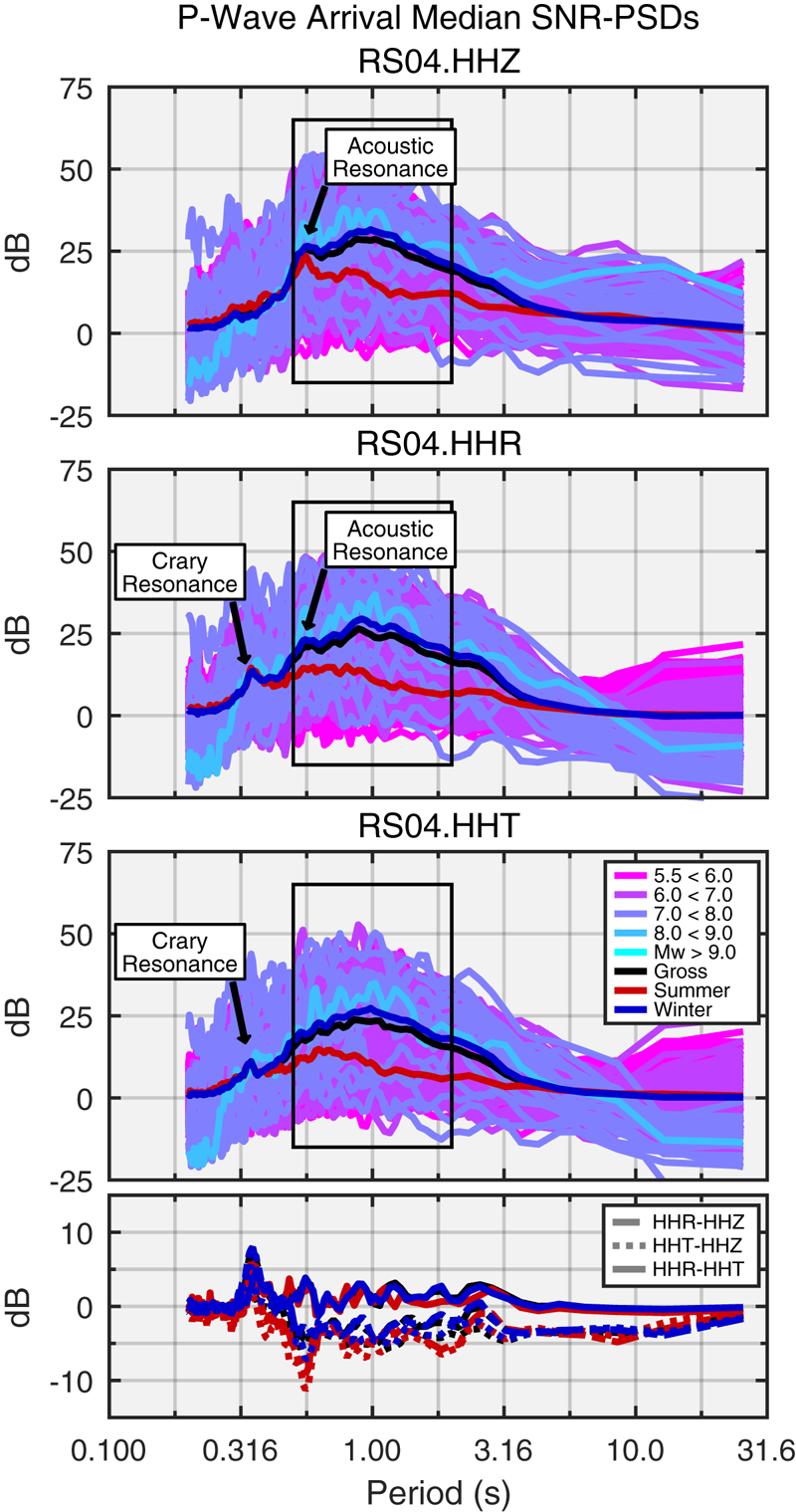
Fig. 6. Median SNR-PSDs for all teleseismic P-wave arrivals recorded at floating station RS04. Acoustic resonances are apparent on the vertical (HHZ) and radial (HHR) components. Crary resonances are observed on the radial (HHR) and transverse (HHT) components. The bottom panel shows the differential PSDs. The periods of these peaks (manually selected) at each floating station were used with Eqn (3) and Table 2 to estimate the ice and water thicknesses shown in Table S1. SNR-PSDs were not smoothed for this process (to maintain spectral resolution) but were scaled by distance and magnitude using Eqn (1).
To account for the low velocity meteoric firn layer, the resonance period PR (Eqn (3)) may be determined as the summation of a glacial ice layer of unknown thickness h′ and a firn layer of assumed known thickness F. The firn layer should also be accounted for in the calculation for orthometric elevation, e:

where h = h′ + F is the total ice shelf thickness.
Figure 7 and Tables S1 and S2 present these results for all RIS/DRIS floating stations and compares them to values from the ROSETTA (Das and others, Reference Das2020), BedMachine (Morlighem and others, Reference Morlighem2020) and BEDMAP2 (Fretwell and others, Reference Fretwell2013) datasets. ROSETTA values are based on airborne gravimetric and ice-penetrating radar. BedMachine is an update of BEDMAP2 with improved resolution of bedrock features derived from algorithmic interpolation, and additionally incorporates REMA (Howat and others, Reference Howat, Porter, Smith, Noh and Morin2019) measurements of RIS orthometric elevations and buoyancy-derived ice thicknesses compiled from multiple sources of airborne and satellite altimetry. BEDMAP2 water column depths were derived from satellite-based gravimetric mapping of sub-RIS bathymetry. BEDMAP2 ice shelf thicknesses were inferred from satellite radar altimetry of orthometric elevation using hydrostatic buoyancy and accounted for a meteoric firn layer of geographically variable thickness (Griggs and Bamber, Reference Griggs and Bamber2011). BEDMAP2 is included for historical perspective, but is expected to be less accurate than ROSETTA and BedMachine.
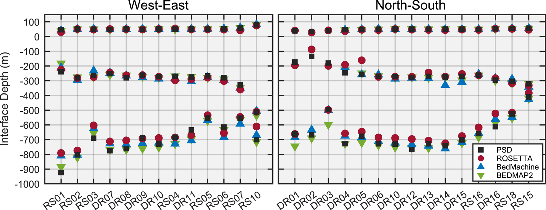
Fig. 7. Orthometric elevations for RIS vertical structure boundaries, as measured at the floating ice RIS/DRIS stations using teleseismic wavefield resonances (‘PSD’). Interpolated values from the ROSETTA (Das and others, Reference Das2020), BedMachine (Morlighem and others, Reference Morlighem2020), and BEDMAP2 (Fretwell and others, Reference Fretwell2013) datasets are provided for comparison. The top, middle and bottom horizons mark the ice free surface, the ice shelf base and the seafloor, respectively. Source values are listed in Tables S1 and S2.
4.2. S-waves (10–15 s)
Theoretically, floating ice-sited seismometers are incapable of directly observing teleseismic S-wave arrivals due to the inability of the underlying water column to propagate shear stresses. Nonetheless, the floating stations of the RIS array did record signals in the 10–15 s period band, coincident with ak135-predicted arrival times for teleseismic S-waves. These signals were recorded most reliably for moderate magnitude (M w > 6.0), low-noise (winter) events such as shown in Figure 3. These S-wave-associated arrivals exhibited strong vertical polarization, similar to the 10–20 s period P-wave arrivals.
A lack of horizontal signal coincident with vertical signal is consistent with a transition of the water column from compressible to incompressible behavior (see Supplementary material). Horizontal energy, when observed, was delayed by up to tens of seconds from the predicted S-wave arrivals, increasing with station distance from the RIS grounding zones (e.g. Fig. 3, red arrows). For comparison, signals from the same event at a grounded RIS station are shown in Figure 4.
Figure 8 shows spatial and seasonal variations in the mean SNR for teleseismic S-wave arrivals in the 10–15 s period band. As detailed in Section 2.3, the noise component for this figure is comprised of 200 s of pre-S-wave arrival time data. The S-wave SNR is therefore referenced against the extended P-wave coda, rather than the pre-event noise as in Figures 3 and 4.

Vertical component SNRs along the W–E transect were nearly uniform at 3–5 dB for most floating and grounded stations during summer and winter (Fig. 8a). For the N–S transect (Fig. 8b), winter vertical SNR was 3–4 dB and was relatively insensitive to distance from the ice front, while summer SNR was a relatively more variable 3–6 dB and showed slight increases with distance from the ice front. The ice front stations DR01–DR03 (represented by DR02 on Fig. 8b) recorded vertical SNRs of <1 dB during winter and summer.
Horizontal component floating station SNRs along the W–E transect decreased with station distance from the grounding line. Radial component (HHR) SNR during winter reached a maximum of 10 dB for floating stations <100 km from the grounding lines (Fig. 8a, RS01, RS07 and RS10), similar to SNR values observed for the grounded stations on Roosevelt Island and in Marie Byrd Land. Floating station radial component SNR decreased at a rate of 0.03 dB km−1 toward the RIS interior, reaching a minimum of 2 dB at RS04. Summer radial SNR followed similar trends, peaking at 7 dB near the shelf margins (somewhat lower than the grounded station values of 10 dB) and decreasing at a rate of 0.02 dB km−1 to a minimum of 2 dB at RS04. Transverse component (HHT) SNRs showed similar spatial distributions as the radial component for floating and grounded stations during winter and summer, although at some stations the transverse SNR was up to 2 dB greater than the radial. Along the N–S transect, floating station radial and transverse component SNRs were generally equivalent and showed <1 dB of change between summer and winter (Fig. 8b). Horizontal SNRs during both seasons increased with distance from the ice front at a rate of 0.02 dB km−1.
4.2.1. Coupling between teleseismic S-waves and Lamb waves
Longitudinal stresses applied to an ice shelf margin have the potential to generate symmetric Lamb wave modes (e.g. Viktorov, Reference Viktorov1967; Rose, Reference Rose1999). Chen and others (Reference Chen2018) showed that ocean gravity waves impacting the RIS ice front generate fundamental mode symmetric (S0) Lamb waves with a propagation velocity of 3.2 km s−1, in agreement with theoretical predictions for RIS thickness, density and elastic properties.
Figure 9 shows a representative record section for S-wave arrivals from an M w 6.6 earthquake in the Java Sea. Serendipitously, the epicenter of this event and the W–E transect were within 1° of a common great circle arc. The grounding lines at Ross Island and Roosevelt Island are nearly perpendicular to this great circle, yielding a favorable polarization alignment between the teleseismic SV-waves and the resulting RIS-propagating S0 Lamb waves (Eqn (6), φ ≈ 0°). Arrival times for the Lamb waves shown in Figure 9 indicate a propagation velocity of 3.2 km s−1 for waves radial from Ross Island and 3.3 km s−1 for waves anti-radial from Roosevelt Island. Particle motions (Fig. 10) are retrograde in the vertical/radial plane and highly elliptical in the radial direction, consistent with theoretical descriptions of symmetric Lamb waves (Viktorov, Reference Viktorov1967). Figure 11 shows the attenuation of Lamb wave amplitude with distance from the grounding lines and is notably similar to the horizontal SNRs in Figure 8. Figure S9 shows a similar record section for an inferred SH-Lamb conversion from the grounding line of Roosevelt Island.
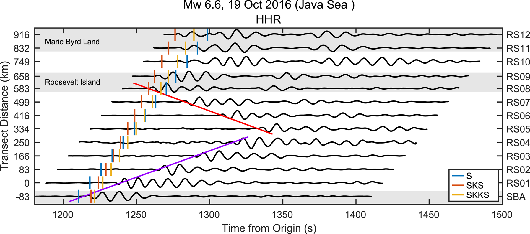
Fig. 9. Radial component ground velocity record section for teleseismic S-waves arriving from the 19 October 2016, M w 6.6 Java Sea earthquake (hypocenter depth: 614 km). Stations and event epicenter are within 1° of a common great circle arc. The purple and red lines mark the (manually fit) travel time curves for S0 Lamb waves generated by SV-wave incident at the grounding lines at Ross (3.2 km s−1) and Roosevelt (3.3 km s−1) Islands, respectively. Ground velocity data were bandpass filtered at 10–15 s and were self-normalized for clarity. Gray areas denote regions of grounded ice. Body wave arrival times were predicted with ak135.
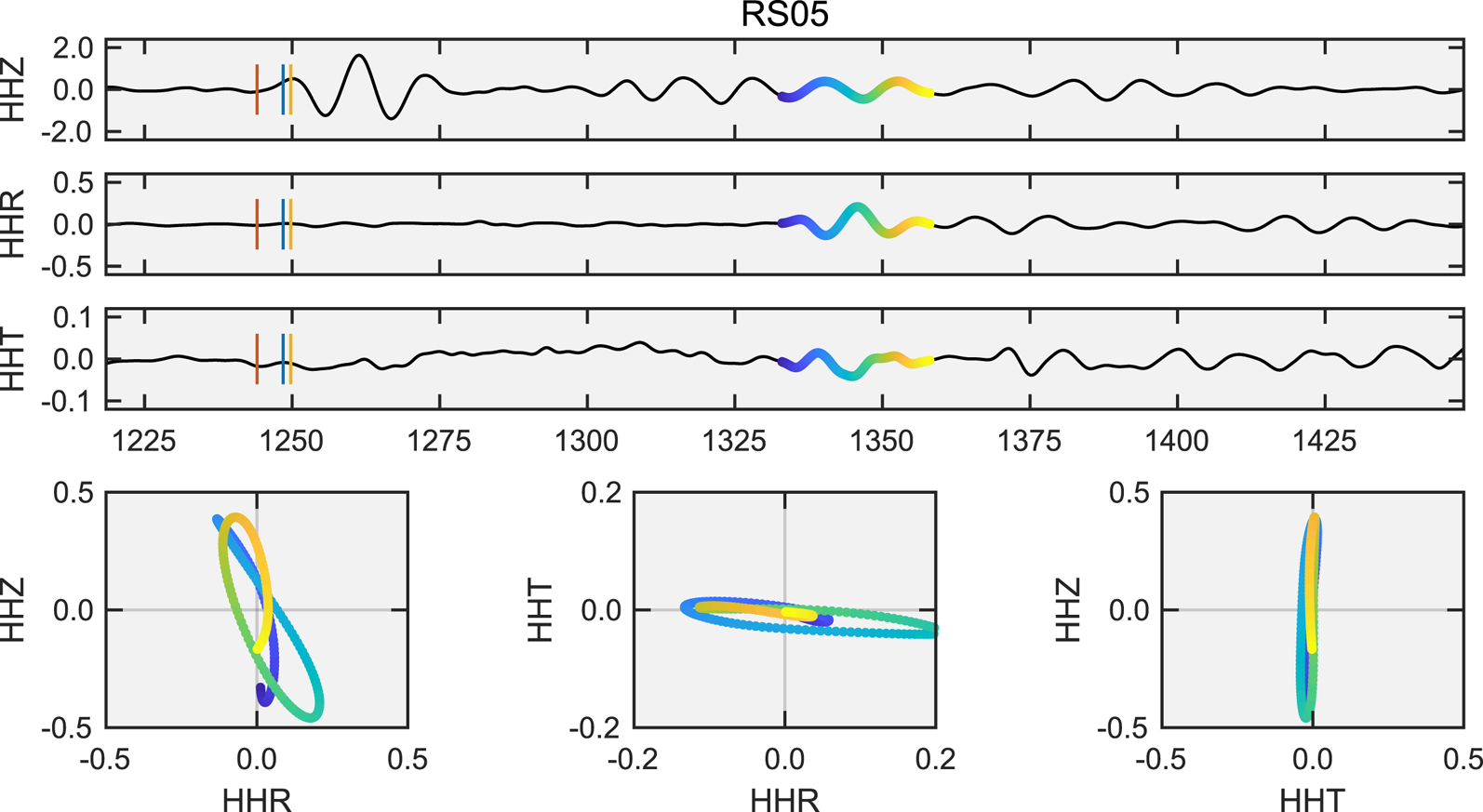
Fig. 10. Three-component ground velocities and particle motions (μm s−1) at floating station RS05 for the earthquake described in Figure 9. The identified Lamb wave arrival and associated particle motions are highlighted by the 25 s of multi-colored trace. Clockwise particle motions in the radial/vertical (HHR/HHZ) plane are consistent with an S0 Lamb wave with expected retrograde particle motions (Viktorov, Reference Viktorov1967; Rose, Reference Rose1999) propagating in the anti-radial direction from the grounding line at Roosevelt Island (Fig. 9, red travel time curve). Motion on the vertical component is dominated by the solid-Earth S-wave coda; S0 Lamb waves are otherwise expected to be radially polarized.
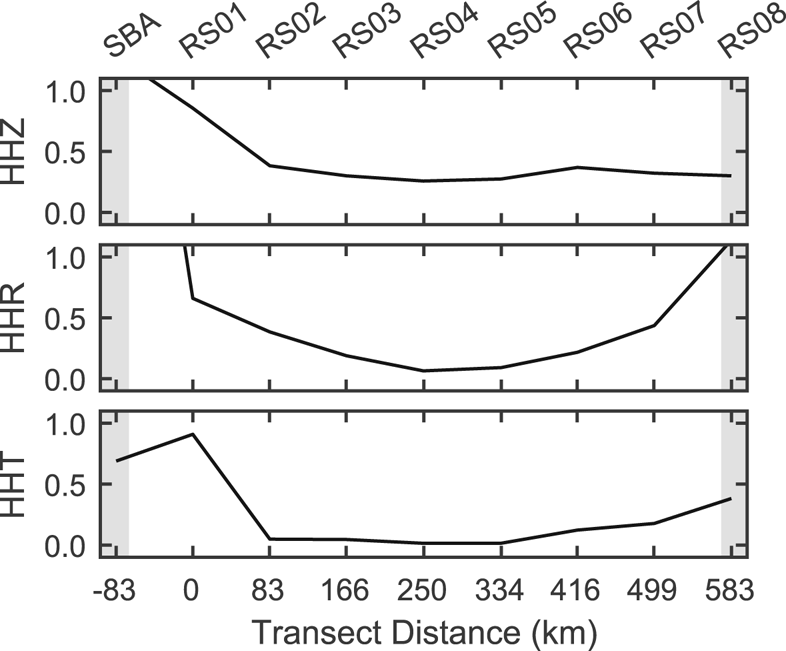
Fig. 11. Root-mean-squared (RMS) ground velocity amplitudes (μm s−1) for the Lamb waves identified in Figure 9. RMS values are based on 25 s of Lamb wave arrival, similar to Figure 10. Radial component RMS at SBA was 4.7 μm s−1; RS08 was 1.14 μm s−1. Gray backgrounds indicate approximate areas of grounded ice.
4.3. Surface waves (13–25 s)
Surface wave arrivals at floating stations with periods longer than the acoustic cutoff period are most strongly observed on the vertical channel; again, see Figures 3 and 4 for a representative comparison of floating and grounded stations, respectively. Velocity dispersion is measurable on vertical component spectrograms even for moderate magnitude (M w > 6.0) earthquakes, particularly during winter (Fig. 3).
Figure 12 shows spatial and seasonal variations in the mean SNR for teleseismic surface wave arrivals in the 13–25 s period band. The ‘signal’ for this figure incorporates 4–2 km s−1 arrivals. The ‘noise’ uses an equal length of pre-4 km s−1 noise, which includes the P- and S-wave codas and some amount of pre-event background noise.

Surface wave SNRs saw significant seasonal variations in absolute and relative component magnitudes. For floating stations along the W–E transect (Fig. 12a), winter vertical SNRs were improved by 3–6 dB over summer values, with the greatest increases observed over stations with the thinnest ices and thickest water columns. At grounded stations, winter vertical SNRs were <2 dB greater than summer values. The radial component SNR at floating stations was 2 dB greater than the transverse component. Summer radial and transverse SNRs at floating stations were nearly equivalent. At grounded stations, during both winter and summer, radial SNRs were consistently 3–4 dB higher than transverse SNRs. Both radial and transverse SNRs improved by <1 dB during winter. For the N–S transect (Fig. 12b), seasonal variations were generally similar to the W–E transect.
Surface wave SNRs also displayed systematic geographic variations. Along the W–E transect (Fig. 12a), floating station vertical SNR was highest in the east at RS07 and lowest in the west at RS01, decreasing by ~0.01 dB km−1 during winter and summer. In contrast, horizontal SNRs were highest near the grounding lines (i.e. RS01 and RS07) and lowest near the RIS centerline (i.e. RS04). During winter, both radial and transverse SNR decreased most rapidly with distance from Roosevelt Island (0.02 dB km−1, RS07–RS04) than from Ross Island (0.01 dB km−1, RS01–RS04). During summer, horizontal SNRs were uniformly 2.5 dB at most floating stations. Exceptions were RS07 and RS10, which both recorded SNRs that were 1.5 dB higher than RS01–RS06.
Along the N–S transect (Fig. 12b), floating station SNRs generally increased with distance from the ice front. For all seasons and all components, SNR at ice front station DR02 was effectively 0 dB. During winter, vertical SNR increased by 0.08 dB km−1 between DR02 and DR10, and by only 0.004 dB km−1 between DR10 and RS18. Summer vertical SNR increased by 0.04 dB km−1 between DR02 and RS16, and was equal to winter SNRs for RS16 through RS18. Horizontal SNRs increased uniformly between DR02 and RS18. During winter, the radial and transverse components each increased at 0.01 dB km−1; during summer, both horizontal components increased at 0.006 dB km−1.
4.3.1. Rayleigh wave group velocities
Figure 13 shows Rayleigh wave group velocities for the sub-RIS crust along portions of both transects, following the multiple filter methods of Dziewonski and others (Reference Dziewonski, Bloch and Landisman1969) and Meier and others (Reference Meier, Dietrich, Stöckhert and Harjes2004). For the W–E transect, we use a station pair of SBA on Ross Island and RS08 on Roosevelt Island; this limits the dispersion analysis to the portion of the West Antarctic Rift System directly beneath the RIS and excludes any influence from the thicker crustal province in Marie Byrd Land (i.e. RS11–RS14). For the N–S transect, we use a station pair of RS04 and RS18, restricted by the degradation of surface wave SNR at stations <130 km from the ice front. We limited source earthquakes to back azimuths within ± 5° of their respective transect great circles and manually selected events for high signal to noise. The W–E analysis used four events from the Nazca subduction zone; the N–S analysis used seven events from the New Zealand subduction zone. Unsurprisingly, the floating stations of the N–S transect yielded a considerably higher median absolute deviation than the grounded stations of the W–E transect. Nonetheless, both transects yielded similar dispersion curves in the low-error 17–23 s period band.
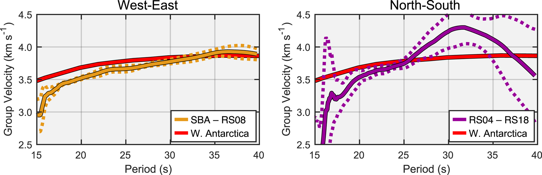
Fig. 13. Representative regional Rayleigh wave group velocities along the RIS transects, determined from cross-correlation of multiple filter analyses for the indicated station pairs (Dziewonski and others, Reference Dziewonski, Bloch and Landisman1969; Meier and others, Reference Meier, Dietrich, Stöckhert and Harjes2004). The W–E curve is the median of four events from the Nazca subduction zone; the N–S curve is the median of seven events from the New Zealand subduction zone. Dashed lines indicate the Median Absolute Deviations. Data have been smoothed with a 21-point rolling average filter. Red curves are representative group velocities for West Antarctica from Shen and others (Reference Shen2017).
5. Discussion
5.1. P-waves (0.5–2.0 s)
For the teleseismic P and immediate coda wavefield, differences between the summer and winter SNR values could technically reflect selection biases in our earthquake catalog (i.e. the signal) or actual variations in the ambient noise field of the RIS. However, since our winter and summer event populations are generally reflective of global earthquake rates (Fig. S2), and given previously documented seasonal background variations (below), we exclude selection bias as a significant contributor to the seasonal SNR variation. Baker and others (Reference Baker2019) examined temporal–spatial variations in ambient noise on the RIS in the 0.4–4.0 s period band and found that onset and termination of the summer high-noise state were strongly correlated with the breakup and redevelopment of contiguous sea ice in the Ross Sea. They suggest that this ‘Tertiary’ noise band, which overlaps with the teleseismic P-wave band, is recording short-period microseisms generated by nonlinear wave–wave interactions (e.g. Ardhuin and Herbers, Reference Ardhuin and Herbers2013), consistent with similar short-period peaks studied elsewhere in Antarctica (Anthony and others, Reference Anthony2015, Reference Anthony, Aster and McGrath2017). The spatial and seasonal variations presented here in Figure 5 do generally mirror the analogous plot for the Tertiary band presented in Baker and others (Reference Baker2019). We therefore conclude that the Tertiary band noise field is the predominate source of noise for summer P-wave observations. Resonances excited by teleseismic signals interacting with the RIS vertical structure (e.g. Fig. 6) are narrow band and low power, relative to the primary signal, and should be easily mitigated with band reject filtering for passive teleseismic applications.
Winter SNR values are generally equivalent between floating and grounded stations (excluding ice front stations DR01–DR03). Summer SNR may be improved by increasing the minimum event magnitude threshold, at the expense of the corresponding decrease in available events (Fig. S2). In either case, SNR values at floating-ice-sited seismographs are generally adequate for passive imaging methodologies, with the significant caveat that only the vertical component conveys information about structural velocities of the crust or mantle. Teleseismically-derived energy in this band observed on horizontal components is the result of P-to-S conversions at the water/ice interface, scattering from internal shelf structure, or is conveyed into the ice shelf wave guide through excitation at the grounding line (see below). Consequently, receiver function or similar converted wave analyses would be useful only for estimating velocity structures within the ice shelf. Vertical component autocorrelation analysis (e.g. Sun and Kennett, Reference Sun and Kennett2016; Pham and Tkalčić, Reference Pham and Tkalčić2018), however, may prove useful for constraining deeper structure.
5.1.1. Estimates of layer thicknesses from resonance periods
Our PSD-derived estimates of RIS ice and water layer thicknesses are generally in agreement with the interpolated ROSETTA and BedMachine values (Fig. 7 and Tables S1 and S2). Admittedly, our method is vulnerable to error from a number of sources, including incorrect elastic parameters, non-planar ice/water and water/seafloor interfaces, seasonal variations in ice thickness due to basal freezing and thawing, and possible changes in near-station bathymetry as the stations moved up to 1 km a−1 with the flow of the ice shelf. Our assumed firn layer thickness of 75 m is based on empirical measurements from the center of the RIS (Diez and others, Reference Diez2016) and may not be appropriate for all stations; RS01, for example, was sited on thinner ice than all other stations and also yielded the largest deviation in ice thickness from all three comparative datasets. ROSETTA had significant data gaps in the vicinity of the RIS/DRIS transect intersection (RS04 and DR04–DR15) which may have introduced significant interpolation errors.
Table S1 presents the most complete survey of RIS/DRIS floating station ice and water column thicknesses. Prior measurements based on ambient noise reverberations (Diez and others, Reference Diez2016; Chaput and others, Reference Chaput2018) were limited to the small aperture DRIS array.
The fidelity of our results to ROSETTA and BedMachine values further supports the development of ice shelf-deployed seismometers as integrated geophysical observatories. Seismometers can provide continuous, long-term monitoring of ice shelf elastic parameters (and thus inferred state-of-health) at significantly less expense and environmental impact compared to aerial or satellite-based remote-sensing surveys; while the latter are capable of greater spatial coverage, they typically do so with greatly reduced temporal resolution. Additionally, planned deployments of unmanned probes to extra-terrestrial ice shelves (e.g. Europa) are also expected to utilize seismometers for initial measurements of vertical structure (Stähler and others, Reference Stähler2018).
5.2. S-waves (10–15 s)
We interpret signals observed at floating stations during the S-wave arrival window as a combination of secondary wavefield effects resulting from interactions of teleseismic S-waves with the sub-shelf seafloor and the shelf grounded margins.
Signal recorded on the vertical component is explicable as S-to-P conversions at impedance contrasts within the crust or sub-shelf sediments (e.g. Beaudoin and others, Reference Beaudoin, ten Brink and Stern1992; Diez and others, Reference Diez2016). The lack of horizontal signal coincident with these S-to-P vertical arrivals (Fig. 3) implies that the S-to-P converted waves couple into the water column as acoustic-gravity waves, as expected for steeply incident waves with periods longer than the acoustic cutoff (Eqn (4)). As previously noted, vertical motions associated with the propagation of acoustic-gravity waves are predominantly incompressible and therefore would not generate significant S-wave modes in the ice. The relatively uniform vertical SNR along the W–E transect may indicate that the S-to-P conversion for floating and grounded stations occurs at the same impedance contrast (e.g. the sediment/basement interface); this is, however, entirely speculative and we acknowledge that the uniformity may instead be an unidentified artifact.
The composition of post-S arrival signals on the horizontal components varies with proximity to the grounding lines, as is evident from the changing ratios between radial and transverse SNRs. In the RIS interior, such horizontal energy is interpreted to be dominated by plate waves generated by teleseismic S-waves coupling at the grounding zones, with additional signal perhaps arising from acoustic-gravity modes. Figure 3, for example, shows two discrete and delayed arrivals on the horizontal components (red arrows), consistent with a symmetric S0 Lamb wave generated by the arrival of the teleseismic SV wave at the southeastern margin of the RIS (HHR) and by SH-waves incident along the southwestern margin (HHT). Horizontal power in these signals is found to increase systematically with proximity to the grounded margins, indicating that these plate waves undergo significant attenuation and/or geometrical spreading in the ice shelf. The stations closest to the grounding lines may also observe teleseism-induced elastic wave energy that is scattered into the ice shelf as incoherent, subcritical (i.e. highly lossy) reverberations. These reverberations, if arriving during the signal integration window, would technically increase SNR even while potentially obscuring the direct teleseismic signal. The discrepancy in HHT SNR between the western and eastern ends of the transect (Fig. 8a) may reflect the greater ice thicknesses in the east, which would allow a greater spectrum of periods and ray parameters to couple into the shelf as resonance modes.
Baker and others (Reference Baker2019) showed that the annual formation of sea ice in the Ross Sea during the winter months depresses noise in the 10–15 s period range by as much as 30 dB across all seismic components. In contrast, our present analysis found no significant seasonal variation in vertical SNR for energy associated with teleseismic S-wave arrivals, indicating that the long period P-wave coda is the most significant noise source for vertical component observations of teleseismic S-waves. Similarly, we found that the significant reductions (relative to summer) in horizontal noise during winter sea ice conditions were not accompanied by a proportionate increase in horizontal SNR.
5.2.1. Coupling between teleseismic S-waves and Lamb waves
Our initial observations of 10–15 s period S0 Lamb waves propagating along the W–E transect suggests a maximum range of ~250 km (Figs 9, 11, S9). In contrast, prior observations of similar period S0 Lamb waves propagating along the N–S transect suggested a maximum range in excess of 450 km, limited by the coverage of the RIS/DRIS array (Chen and others, Reference Chen2018; Baker and others, Reference Baker2019).
This disparity may be reflective of the large scale structure of the RIS. As with other elastic waves, Lamb waves are readily scattered by structural defects oriented perpendicular to wave propagation, such as open cracks or impedance contrasts (Viktorov, Reference Viktorov1967; Rose, Reference Rose1999). Examples of defects present in the RIS include open rifts, and highly strained regions of ice such as suture zones and shear zones, where ice densities or compositions may be laterally heterogeneous. Mapping of RIS surface textures indicates that shear and suture zones are present in the RIS as north-south oriented fabrics (LeDoux and others, Reference LeDoux, Hulbe, Forbes, Scambos and Alley2017), consistent with the greater Lamb wave attenuation (via scattering) observed along the W–E transect. Tensional rifts are also present near the RIS ice front but are located off-axis from the N–S array transect and therefore would not affect the studied Lamb waves, except as possible loci of scattered energy.
An alternate explanation is that the ocean wave-induced Lamb waves simply have greater initial amplitudes than the teleseism-induced Lamb waves identified in Figure 9; that is, our inference of lateral anisotropy may be based on insufficient sampling of teleseism-induced Lamb waves. A conclusive test for Lamb wave anisotropy would be a comparison of attenuation curves along each transect, requiring a greater number of teleseism-induced Lamb wave observations than we have currently identified. Compilation of such a catalog could be based on travel time predictions and eigenvector decomposition (Vidale, Reference Vidale1986) to verify that waveform polarizations satisfy Eqns (6–8).
5.3. Surface waves (13–25 s)
Signals observed by floating stations during the surface wave arrival window are often overwhelmingly on the vertical channel and have dispersion relations comparable to those of nearby grounded ice stations (e.g. Figs 3, 4). This behavior is consistent with the general model we have established for the interactions of solid Earth elastic waves with the RIS and the sub-shelf water column. That is, we expect that long period (>13 s) teleseismic Rayleigh waves propagating beneath the RIS should couple with the water column and the ice shelf as, predominately, incompressible vertical displacements; horizontal signals at the seafloor should not be observed above the water column. Semblance between the vertical component dispersion curves at floating and grounded stations further indicates that the RIS floating stations directly observed teleseismic Rayleigh wave arrivals. Similar observations of teleseismic Rayleigh waves on a free-floating tabular iceberg were presented in Okal and MacAyeal (Reference Okal and MacAyeal2006) for the 2004 and 2005 Sumatra earthquakes (M w 9.1 and 8.6, respectively).
Signals coincident with surface wave arrivals are weakly observed on the horizontal components during the winter low-noise state, with generally higher SNRs on the radial component than the transverse (Figs 3, 12). We suggest two non-exclusive mechanisms. The perhaps more obvious explanation is the propagation of plate wave modes from the grounding line via the same excitation processes as observed for S-wave arrivals. This would account for both radial (Lamb) and transverse (shear horizontal plate) signals. The decreasing horizontal SNRs with increasing distances from the grounding lines (Fig. 12a) would also be consistent with attenuation of these plate wave modes. For the radial component, S0 Lamb waves propagate across the RIS at 3.2 km s−1 (Fig. 9), in comparison with 3.5 km s−1 for crustal Rayleigh waves (Fig. 13), allowing for roughly similar arrival times between vertically polarized Rayleigh waves and radially polarized Lamb waves (Fig. 3). Shear horizontal plate waves would be restricted to the fundamental mode at these long periods and would propagate at the S-wave velocity of the RIS, β i (Rose, Reference Rose1999).
An alternate explanation is that the radial signal is the result of acoustic Rayleigh leakage into the water column. A Rayleigh wave traveling along a solid/liquid interface will lose energy to the liquid medium at a rate of e −1 per ten wavelengths if the acoustic velocity of the liquid, αw, is less than the phase velocity of the Rayleigh wave, V R (Viktorov, Reference Viktorov1967). These so-called ‘leaky’ Rayleigh waves emit acoustic waves at angles of incidence greater than the Rayleigh angle, θ R = sin−1(αw/V R) (Glorieux and others, Reference Glorieux2002). For V R = 3.5 km s−1, θ R = 24.5°. Acoustic waves are post-critical at the water/ice interface for this angle and convert >80% of their energy into SV-waves within the ice (Fig. S3). It is beyond the scope of this study as to how leaky Rayleigh wave energy would interact in detail with acoustic-gravity wave phenomena, but we expect that the elastic energy of such a mode would be increasingly favored with increasing angle of incidence. However, the strength of the apparent relation between horizontal SNR and distance from the grounding line (Fig. 12a) suggests that any effect of sub-shelf Rayleigh wave leakage is secondary to the plate modes.
Generally, we do not expect to observe sub-shelf crustal Love waves at floating stations. Steeply sloping bathymetry may, in theory, cause leakage of Love wave energy into the water column. However, we have observed no clear evidence of such signals.
Ambient noise in the 13–25 s period band is a multi-mode wavefield driven by the impacts of ocean swell with the RIS ice front, as described by Baker and others (Reference Baker2019). For their analysis, Baker and others restricted their so-called 'Primary' band to periods of 10–20 s, keeping with the traditional bandpass of the primary microseism wavefield. However, the PSDs included there indicate that the summertime high-power state for this wavefield is actually observed at periods as long as 30 s. As such, we have adjusted the noise calculations from that study to the 13–25 s period band and have included the results in Figure S13; we stress that this updated figure merely adjusts the quantitative distributions and does not otherwise change the qualitative interpretations.
We note some similarities between the spatial and seasonal distributions of vertical component surface wave SNR and Primary band noise. As noted by Baker and others (Reference Baker2019), the predominant source of noise for the RIS throughout the year in this general period band is ocean gravity waves. During the summer open water months of the Ross Sea, ocean gravity waves generate ambient noise via direct interaction with the ice front and penetration into the sub-shelf water cavity; these forcings remain observable throughout winter, even in the presence of extensive sea ice. Along the N–S transect, both summer and winter vertical component SNRs (Fig. 12b) are generally inverted from the adjusted Primary band noise powers (Fig. S13b). This indicates that, consistent with Baker and others (Reference Baker2019), the vertical noise wavefield in the 13–25 s period band is driven by a combination of ocean gravity waves and primary microseism Rayleigh waves. Ocean gravity waves are the predominant forcing within 130 km of the ice front during winter and within 250 km during summer, while primary microseism Rayleigh waves are responsible for the wavefield at greater distances. Variations in vertical SNR along the W–E transect (Fig. 12a) are similarly inverted with respect to the primary microseism noise band trend (Fig. S13a); this is explained by the decreased flexural rigidity of the thinner ice near Ross Island, which in turn allows for larger amplitude flexural-gravity waves.
6. Summary and conclusions
We present a signal-to-noise and phenomenological analysis of 2 years of teleseismic earthquake signals recorded by a 34-station broadband seismic array deployed across the RIS, Antarctica. Teleseismic observations in this environment must contend with a complex elastic and gravity wave displacement wavefield consisting of: (1) short period (0.4–4.0 s) ocean noise associated with shorter period microseism generation and/or direct ice front excitation; (2) primary and secondary microseisms; (3) flexural-gravity waves excited by infragravity and ocean swell waves; (4) water layer-decoupled P- and S-wave arrivals; (5) high-frequency (1–10 Hz) reverberations from the strong ice shelf basal and surface impedance contrasts and (6) intermediate to long period (10–50 s) plate waves induced by oceanic and teleseismic forcings. The ocean-forced components of this ambient wavefield have a strong dependence on sea ice extent in the Ross Sea, resulting in bimodal noise distributions between ‘winter’ (1 April–30 November) and ‘summer’ (1 December–31 March) sea ice periods (Baker and others, Reference Baker2019).
We use 300–400 teleseismic earthquakes to generate band-averaged SNRs for P-wave (0.5–2.0 s), S-wave (10–15 s) and surface wave (13–25 s) arrivals and codas, as recorded at floating- and grounded-ice-sited seismometers. We also address secondary wavefield effects, such as P-wave-derived intralayer resonances, S-wave-derived symmetric mode Lamb waves, and the effects of incompressible displacement of the sub-shelf water column by long period/long wavelength solid Earth elastic waves.
Teleseismic P-wave arrivals were well-observed at the RIS floating stations throughout the year. During the winter low-noise state, three-component P-wave SNRs at floating stations were uniformly equivalent to observations at nearby grounded stations (20–25 dB); an exception was stations within 3 km of the RIS ice front, where vertical and horizontal SNRs were 5 and 10 dB lower, respectively. During the summer high-noise state, three-component SNRs were effectively 0 dB at the ice front and increased by 0.05 dB km−1 landward; extrapolating from these trends suggests that summer SNR values would reach winter SNR values at 460 km from the RIS ice front. Given the similarity between floating and grounded station SNR values, we conclude that teleseismic P-wave coda may be useful to passive imaging methods for the determination of structural velocity within the ice shelf (vertical and horizontal components) and the sub-shelf crust and mantle (vertical component, only).
Teleseismic P-wave arrivals contain elastic wave frequencies that are optimal for generating fundamental mode resonances within the ice shelf and the sub-shelf water column. We used the peak periods of these resonances – which are readily apparent on PSD plots of earthquake arrivals – in conjunction with the mean ray parameter to estimate ice shelf and water column thicknesses. Our results agree with interpolated BedMachine estimates of ice and water thicknesses (Morlighem and others, Reference Morlighem2020) to within 7%. This demonstrates that long-term deployments of seismometers to terrestrial or extra-terrestrial (e.g. Europa) ice shelves have potential for year-round monitoring of ice shelf thicknesses and possibly even initial estimates of unknown vertical geometries.
Teleseismic S-wave codas were generally poorly recorded (<5 dB SNR) at all floating stations throughout the year. However, we do show that these arrivals, when incident near the RIS grounding lines, generate symmetric mode Lamb waves that may be observed at least 250 km into the interior the ice shelf. Significantly, the travel times and attenuation of these common teleseismically excited Lamb waves could be exploited for large scale, wide-angle measurements of ice shelf properties using the same techniques already perfected by the field of ultrasonic non-destructive testing.
Teleseismic Rayleigh wave arrivals were generally well-observed (>10 dB SNR) on the vertical components of floating stations, particularly during the winter, but were poorly observed (<5 dB) on the radial components. A similar deficit (relative to grounded stations) between vertical and radial power was also observed for long period P-wave arrivals (>20 s). We attribute this phenomena to the shallow-water acoustic cutoff period (~2.0 s), above which solid Earth elastic waves are expected to couple into the water column as incompressible vertical displacements. Such a displacement of the water column would not generate a P-to-S converted phase at the water/ice interface. Notably, these vertical displacements do preserve the Rayleigh dispersion values and may be exploited to determine the sub-shelf crustal Rayleigh wave group velocity curves. Our initial attempt at calculating group velocities between a pair of floating stations yielded similar values in the 17–23 s band as also determined for a pair of grounded stations. Unfortunately, the floating station analysis developed significant and unattributed errors at periods longer than 25 s and diverged from the grounded station fit.
In addition to quantifying teleseism metrics and signal character on the RIS, we note widely observed wave phenomena that can be applied for spatial and temporal studies of the elastic state of ice shelves. In particular, the presence of spectral resonances that can be utilized to estimate local layer thicknesses, and first observations of shelf-spanning, teleseismically induced Lamb waves generated at grounded zones by teleseismic S-waves. With a suitably dense network, observations of these vertical and horizontal wavefields might allow for time-lapse seismic tomography at the ice shelf scale.
Supplementary material
The supplementary material for this article can be found at https://doi.org/10.1017/jog.2020.83.
Acknowledgments
This research was supported by NSF grants PLR-1142518, 1141916, 1142126, 1246151, 1246416 and OPP-1744852 and 1744856. Seismic instruments were provided by the Incorporated Research Institutions for Seismology (IRIS) through the PASSCAL Instrument Center at New Mexico Tech. Data are available through the IRIS Data Management Center under RIS and DRIS network code XH (doi.org/10.7914/SN/XH\_2014). We make use of the following supplemental datasets: (1) permanent Global Seismographic Network station SBA (20 Hz) near Scott Base on Ross Island (doi: 10.7914/SN/IU); (2) bathymetric and topographic data from the National Geophysical Data Center ETOPO1 Global Relief Model (doi:10.7289/V5C8276M) and (3) coastline data from the SCAR Antarctic Digital Database (add.scar.org, accessed August 2020). Ice shelf profiles and interpolations of BedMachine and BEDMAP2 data were generated with the Antarctic Mapping Tools (Greene and others, Reference Greene, Gwyther and Blankenship2017). The facilities of the IRIS Consortium are supported by the National Science Foundation under Cooperative Agreement EAR-1851048 and the DOE National Nuclear Security Administration. We thank Samantha Hansen and an anonymous reviewer for suggestions that improved this article.


 Open access