


1. Introduction
In a context of generalized global glacier mass loss, the social and scientific interest about glaciers in mountain regions has increased substantially (Adler and others, Reference Adler, Huggel, Orlove and Nolin2019). The Southern Andes in Argentina and Chile are part of this global pattern of retreat. An increasing number of references indicate that over the past decades, Andean glaciers have lost mass at different and sometimes alarming rates, along this extensive mountain range (e.g. Braun and others, Reference Braun2019; Dussaillant and others, Reference Dussaillant2019; Hock and others, Reference Hock2019b). Basic information on the current state of glaciers is crucial from different points of view, including multi-temporal assessments of ice mass changes and improved analyses of glacier-climate relationships. Updated and better spatial resolution glacier inventories are also critical to outline environmental policies for glacier protection and monitoring programs, as well as for developing mitigation and adaptation strategies in response to climate changes (Johansen and others, Reference Johansen2019).
In 2010, the Argentinean Congress promulgated the National Law 26639 on ‘Minimum Standards Regime for Preservation of Glaciers and Periglacial Environment’. This law established the protection of glaciers and the periglacial environment as strategic reservoirs of water in the solid state, and led to the creation of the National Glacier Inventory (NGI) to identify and characterize glaciers and ice-rich periglacial landforms that act as water storages for protection, management and monitoring purposes. The Argentinean Institute for Snow, Ice and Environmental Sciences of the National Science and Technology Council (IANIGLA-CONICET for the initials in Spanish) was designated as the technical agency responsible for the development and periodic updating of the inventory in collaboration with the National Ministry of the Environment and Sustainable Development. The NGI program put glaciers and periglacial landforms at the forefront of discussions throughout the country and represented an unprecedented attempt to integrate science and policy in Argentina.
The results of the first NGI were officially presented in May 2018, allowing any interested user free access, for the first time in history, to complete, updated, highly detailed and standardized information about ice masses in Argentina. This information is vital for answering many basic questions about the nation's permanent ice masses, for addressing local needs in different regions of the country, and also as a valuable input for glaciological studies along the Southern Andes. Recently, it has been noted the need of more detailed inventories, to include the smallest glaciers (usually under-represented in glacier inventories) for a more accurate estimation of past and present contribution of glacier mass loss to global mean sea level rise (Bahr and Radić, Reference Bahr and Radić2012; Parkes and Marzeion, Reference Parkes and Marzeion2018; Leigh and others, Reference Leigh2019). The aim of this paper is to provide an overview of the methods and results of the first NGI and to establish a comparison between the local and global inventories.
2. Previous glacier inventories in Argentina
In Argentina, there have been several attempts to produce glacier inventories for selected portions of the Andes (e.g. Bertone, Reference Bertone1960; Rabassa and others, Reference Rabassa, Rubulis and Suárez1978; Corte and Espizua, Reference Corte and Espizua1981). These inventories provided important information, but the results were mostly local and followed different objectives and methodologies, which inhibited their compilation into homogeneous and consistent databases. Prior to the publication of the NGI, there were still many gaps of glaciological information along the Andes, even for some sectors with large glacierized areas and many important watersheds (IANIGLA-CONICET, 2010).
The first attempt to produce a glacier inventory in Argentina was conducted in the Argentinean portion of the Southern Patagonian Icefield (SPI), the largest glacierized area in the country. The work was based on aerial photographs and field surveys and only summarized the area and location of the largest glaciers (Bertone, Reference Bertone1960). A few decades later, the inventory of the Mendoza river basin (32.15–33.25° S) in the Argentinean Central Andes represented the first national inventory to follow the UNESCO's recommendations and to include rock glaciers (UNESCO, 1970). This inventory, also based on aerial photographs, characterized clean ice, debris-covered ice and rock glaciers larger than 0.02 km2 (Corte and Espizua, Reference Corte and Espizua1981).
The increased availability of satellite images in the following decades facilitated the development of detailed inventories using semi-automated processes for mapping glaciers in the SPI (Aniya and others, Reference Aniya, Sato, Naruse, Skvarca and Casassa1996; Skvarca and De Angelis, Reference Skvarca and De Angelis2003). Rock glaciers were also mapped in some areas of the Desert Andes and the Central Andes (Ahumada, Reference Ahumada2002; Trombotto, Reference Trombotto2003; Angillieri and Esper, Reference Angillieri and Esper2009; Ahumada and others, Reference Ahumada, Páez and Ibáñez Palacios2013; Martini and others, Reference Martini, Strelin and Astini2013). More recently, the inventories of the Valles Calchaquíes (25° S), Monte San Lorenzo (47° S), and Volcán Domuyo (36° S) areas were published by Falaschi and others (Reference Falaschi, Bravo, Masiokas, Villalba and Rivera2013, Reference Falaschi, Castro, Masiokas, Tadono and Ahumada2014, Reference Falaschi, Masiokas, Tadono and Couvreux2016). Masiokas and others (Reference Masiokas2015) produced a glacier inventory and assessed the recent fluctuations (1979–2015) along the Las Vueltas and Túnel basins, adjacent to the SPI.
3. Regional and climatic setting
The Argentinean Andes extend for ~4000 km (22–55° S) along the southwestern margin of South America. The highest elevations occur in the central and northern portions of this range (22–34° S) with several peaks exceeding 6000 m a.s.l. including the Mount Aconcagua (6961 m a.s.l.), the highest peak in the world outside Asia. The large latitudinal range from subtropical to subantarctic domains, steep elevational gradients and the north-south orientation perpendicular to the prevalent atmospheric circulation cause extremely different climatic conditions, and consequently, a great variety of ice mass types along the Southern Andes.
For the purposes of the NGI, and following the glacio-climatological regions of Lliboutry and others (Reference Lliboutry, Williams and Ferrigno1998), the Argentinean Andes were divided into five glaciological regions. This regionalization is similar to that used for the glacier inventory of Chile on the western side of the Southern Andes (Barcaza and others, Reference Barcaza2017). The Desert Andes region (22–31° S) is located in the northwestern part of Argentina. This region encompasses a high (3500–6700 m a.s.l.) mountain range with arid to semi-arid climatic conditions. Scarce precipitation (<500 mm a−1) is usually concentrated during the austral summer months (Fuenzalida and others, Reference Fuenzalida, Sánchez and Garreaud2005; Viale and others, Reference Viale2019). Farther south, the Argentinean Central Andes (31–35° S) are also characterized by high elevations (2600–6900 m a.s.l.). The region receives modest annual precipitation amounts, increasing southward from ~500 mm at 31° S to 1000 mm at 35° S (Viale and Nuñez, Reference Viale and Nuñez2011). In the Northern Patagonia Andes region (35–45° S), the precipitation amounts increase considerably (>2000 mm) due to the more frequent passage of cyclonic systems embedded in the dominant westerlies (Viale and others, Reference Viale2019). However, the mean elevation of the Andean barrier decreases substantially (1000–1500 m a.s.l.) compared to the northern latitudes. In the Southern Patagonian Andes region (45–53° S) the frequent passage of westerly cyclonic systems throughout the year lead to high annual total precipitation values (>4000 mm) (Bravo Lechuga and others, Reference Bravo Lechuga2019). The presence of relatively higher peaks (some over 3000 m a.s.l.) and elevated plateaus favor the presence of the largest glacier concentration in South America. Finally, the Andes in the Tierra del Fuego region (53–55° S) are substantially lower (1000–1500 m a.s.l.) with a west-east orientation, parallel to the prevalent westerly winds. Thus, the orographic enhancement of precipitation is not as strong as farther north and the precipitation amount diminishes from west to east (Fig. 1).
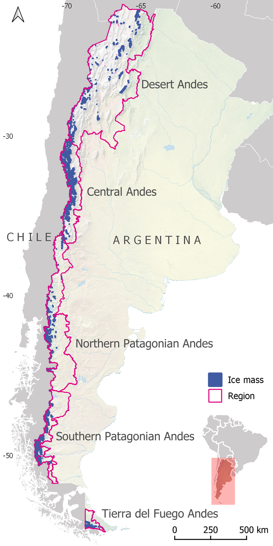
Fig. 1. Ice mass distribution and regions used in the NGI.
4. Data and methods
4.1. Organization of the NGI
The identification of ice masses and their subsequent characterization in a dedicated database was organized and compiled at the scale of hydrological basins. Basins were separated using a semi-automated watershed delineation process based on DEMs with on-screen manual corrections. The freely available SRTM DEM v4 and the ASTER GDEM v2, both voids filled, were used in the process (Jarvis and others, Reference Jarvis, Reuter, Nelson and Guevara2008; Tachikawa and others, Reference Tachikawa, Kaku and Iwasaki2011). Where larger basins were present, they were divided into smaller sub-basins to facilitate the workflow and the organizational scheme of the NGI. Finally, the boundaries of the basins and sub-basins were visually checked against satellite images and manually corrected in certain areas and to comply with the official political national boundary of Argentina. This process resulted in 66 Argentinean Andean basins or sub-basins.
4.2. Ice masses mapping and characterization
The identification and mapping of ice masses, within each of the 66 NGI sub-basins, was based on remote-sensing data, and largely followed the guidelines of the GLIMS project (Rau and others, Reference Rau, Mauz, Vogt, Khalsa and Raup2005; Raup and Khalsa, Reference Raup and Khalsa2010; Kargel and others, Reference Kargel, Leonard, Bishop, Kääb and Raup2014). A total of 178 optical multispectral satellite images of medium spatial resolution (15–30 m) and 224 high spatial resolution (2–5 m) acquired between 2004 and 2016 were used in the inventory. Fifty five percent of the total number of images were used as base images for the inventory, and the rest were used as auxiliary data in cases of snow cover, shadows and clouds and for proper identification of debris-covered ice and rock glaciers. Images coming from different satellites (ASTER, ALOS, SPOT, Landsat, CBERS) were carefully selected considering the absence of seasonal snow and cloud cover, which greatly varies at different latitudes along the Andes (Paul and others, Reference Paul2009) (Fig. 2, Table S1).

Fig. 2. Satellite images used for the NGI. (a) Footprint and number of overlapping scenes used for identifying glaciers and perennial snowfields. (b) Same as (a), but for rock glaciers. (c) Number of scenes per year, classified by satellite, used in the inventory of glaciers and perennial snowfields. (d) Same as (c), but for rock glaciers.
All ice masses larger than 0.01 km2 were included in the inventory, this being a standard threshold in most glacier inventories (Andreassen and others, Reference Andreassen, Paul, Kääb and Hausberg2008; Nicholson and others, Reference Nicholson2009; Paul and others, Reference Paul2009, Reference Paul, Frey and Le Bris2011; Gardent and others, Reference Gardent, Rabatel, Dedieu and Deline2014; RGI Consortium, 2017). Then, based on their superficial characteristics, ice masses were classified into five main operational categories: clean ice, debris-covered ice, glacierets or perennial snowfields, rock glaciers (active and inactive), and debris-covered ice with rock glacier. These main categories were all mapped as individual polygons (Fig. 3).

Fig. 3. Examples of the different types of ice masses mapped in the NGI (field views on the left, and satellite images on the right). (a) Left, clean ice; right, ASTER VNIR; (b) debris covered-ice; ASTER VNIR; (c) perennial snowfield; ASTER VNIR; (d) active rock glacier; (e) inactive rock glacier; ALOS AVNIR; (f) debris-covered ice with rock glacier; ASTER VNIR.
Clean ice and perennial snowfields were automatically extracted using multispectral data. The NDSI (Normalized-Difference Snow Index) was applied when satellite images contained a band in the shortwave infrared (SWIR). This index clearly identifies and separates snow and ice-covered surfaces from barren surfaces making use of the large reflectance difference of these surfaces in the visible and near-infrared bands (VNIR) vs SWIR (König and others, Reference König, Winther and Isaksson2001; Paul and others, Reference Paul, Kääb, Maisch, Kellenberger and Haeberli2002, Reference Paul, Frey and Le Bris2011; Bolch and Loibl, Reference Bolch and Loibl2018). In cases where the satellite imagery lacked the SWIR bands, we used a supervised classification with an object-oriented approach. Following the initial identification of snow and ice-covered surfaces, glacier outlines were manually corrected to include, for example, ice in cast shadow areas. In this classification scheme, small mountain glaciers were separated from perennial snowfields or glacierets by visual interpretation of present or former flow indicators (mainly crevasses or foliation), independently of the size. Flow indicators were identified in high-resolution satellite images, as they are difficult to detect in small ice masses using medium spatial resolution images. When no flow indicators were observed, ice bodies were considered as perennial snowfields (Fig. S1). The perennial condition of snowfields was checked using images of different dates (normally the base image compared to another earlier image with two or more years of difference).
Rock glaciers and sectors of glaciers covered by debris are difficult to identify and map properly using semi-automated methods because the spectral characteristics of these surfaces are very similar to the surrounding landscape. Thus, these units were manually digitized using a combination of medium to very-high spatial resolution images for a more accurate interpretation of the morphological characteristics typical of rock glaciers and debris-covered ice. Some have tried to automate the mapping of these particular surfaces (Bishop and others, Reference Bishop, Bonk, Kamp and Shroder2001; Paul and others, Reference Paul, Huggel and Kääb2004). However, visual interpretation and manual digitization remains the most reliable and widely used procedure for rock glaciers and debris-covered ice (Racoviteanu and others, Reference Racoviteanu, Paul, Raup, Khalsa and Armstrong2009; Scotti and others, Reference Scotti, Brardinoni, Alberti, Frattini and Crosta2013; Jones and others, Reference Jones, Harrison, Anderson and Betts2018). Rock glacier units were mapped using a restricted footprint (i.e. the frontal and lateral talus were not included). In all cases, the area of the rock glaciers was limited to where the creeping of permafrost is evident considering the surface morphology. It is worth noting that in many semi-arid sectors of the Andes there are transitional phases where debris-covered ice gradually transforms into rock glaciers with no clear boundary between these surfaces (Janke and others, Reference Janke, Bellisario and Ferrando2015). These cryoforms were mapped together and included into the ‘debris-covered ice with rock glacier’ category in the database (Fig. S2). Manual digitization of rock glaciers and debris-covered ice was the most time consuming and difficult task, which largely depends on the experience and criteria of the analyst, and to a lesser extent, of the spatial resolution of satellite images. Even with high-resolution images, interpretation may differ from one analyst to another (Paul and others, Reference Paul2013; Brardinoni and others, Reference Brardinoni, Scotti, Sailer and Mair2019).
Many individual polygons in the clean ice and debris-covered ice categories (and for some debris-covered ice with rock glacier) are adjacent to each other and form single units or ice masses. In these cases, these polygons were grouped together and assigned the IDs of the greater unit, but differentiated by their morphological characteristics in the database. In contrast, continuous ice masses belonging to distinct basins were split into individual glaciers according to ice divides using, as in the case of basins, in a semi-automated process based on DEMs with on-screen manual corrections (Bolch and others, Reference Bolch, Menounos and Wheate2010; Paul and others, Reference Paul, Frey and Le Bris2011). All different ice masses were morphologically characterized following the classification scheme of the World Glacier Monitoring Service (WGMS) and the Global Land Ice Measurements from Space (GLIMS) (i.e. primary classification, form, frontal characteristics, longitudinal characteristics, dominant mass source, tongue activity, moraine code 1, moraine code 2, debris coverage of tongue) (Haeberli and others, Reference Haeberli, Bösch, Scherler, Østrem and Wallén1989; Rau and others, Reference Rau, Mauz, Vogt, Khalsa and Raup2005). Few adaptations were made to account for local characteristics of rock glaciers which are not fully developed in the WGMS and GLIMS classification schemes. This expansion of the database allowed a much more detailed morphological description of rock glaciers, which are crucial components of the Andean cryosphere along extensive semi-arid Andean landscapes (Jones and others, Reference Jones, Harrison, Anderson and Betts2018, Reference Jones, Harrison, Anderson and Whalley2019). Some parameters were added to the database to account for the degree of activity, form, origin and structure of rock glaciers in the Argentinean Andes. In addition to these parameters, each unit was classified and characterized according to different information, including general data (local ID, GLIMS ID, province, basin and sub-basin name, common name, latitude and longitude), morphometric details (area, elevation, slope, aspect, length) and information about the satellite imagery (sensor, date) used in the mapping process. In total, the database consists of 38 fields that were carefully checked and filled for each ice mass in the NGI.
4.3. Fieldwork and uncertainty assessment
The mapping results were validated through field campaigns conducted in basins/sub-basins where glaciers, perennial snowfields and rock glaciers were detected through satellite imagery. Three main aspects of the units were assessed in these fieldworks: the identification, the classification according to the operational categories and the outline delineation. Since most ice masses in Argentina are located in remote areas with difficult access, no roads and limited communications, the ice masses and the locations selected for field validation were chosen taking into account the accessibility and security of the personnel who participated in the campaigns (Stumm and others, Reference Stumm, Joshi, Salzmann and MacDonell2017).
Uncertainties in derived outlines were also assessed by multiple digitization (six analysts) of a set of glaciers and rock glaciers (Paul and others, Reference Paul2013, Reference Paul2017). We selected an area containing seven glaciers with clean and debris-covered ice centered at 34.406° S, 70.031° W, and another area with six rock glaciers at 32.9173° S, 69.6753° W. In both cases, these areas exhibit variable debris, shadow and snow conditions. Glaciers were mapped using an ASTER-VNIR (15 m spatial resolution) image from 4 April 2011, whereas for rock glaciers we used an ALOS pansharpened (2.5 m resolution) from 28 March 2010, both from the end of the ablation period in the Southern Hemisphere. It is important to note that for this mapping exercise the analysts were required to map each unit using only the two selected images without the aid of external complementary information.
4.4. Assessment of the differences between the NGI and the Randolph Glacier Inventory
The Randolph Glacier Inventory (RGI), first released in 2012, is a global inventory of glacier outlines. It was initially developed in a short period of time (1–2 years) with limited resources, by a group of international glaciologists to serve the needs of the Fifth Assessment Report of the Intergovernmental Panel on Climate Change (IPCC) (Pfeffer and others, Reference Pfeffer2014). Their aim was to achieve a complete coverage rather than extensive documentary details, and different sources of information, dates, and qualities were merged in one single glacier inventory. Since its release, the RGI has been constantly improved by the ingestion of local to regional glacier inventories until the present version RGI 6.0 (RGI Consortium, 2017) and has become a worldwide reference for glaciological studies (Marzeion and others, Reference Marzeion, Jarosch and Hofer2012; Bosson and others, Reference Bosson, Huss and Osipova2019; Farinotti and others, Reference Farinotti2019; Hock and others, Reference Hock2019a).
Interestingly, the accuracy in terms of number, extent and characteristics of the glaciers included in the RGI have never been adequately evaluated in the Southern Andes. Here we compared the RGI 6.0 with the local glacier inventories of Argentina and Chile (Barcaza and others, Reference Barcaza2017). For this, we combined both datasets into one Southern Andes glacier inventory (hereafter SA inventory). As the RGI 6.0 does not include rock glaciers, we excluded these ice masses (more than 10 000 units) prior to analysis.
Pfeffer and others (Reference Pfeffer2014) acknowledge that RGI dataset could under-record the smaller ice masses (glacierets and other very small glaciers) or over-record by misidentification of small seasonal snowpatches as perennial snowfields (Fig. S4). Thus, only the upper and lower boundaries of the total number of small ice bodies could be given. The SA inventory was compared with both the lower and upper bound of small ice masses’ number in the RGI 6.0 (following Pfeffer and others (Reference Pfeffer2014)) in terms of the number of units, area covered and estimated volume. To calculate the ice volume in the RGI 6.0 and SA we applied the volume-area scaling derived by Huss and Farinotti (Reference Huss and Farinotti2012) for the Southern Andes. Although this empirical relationship underestimates the volume for the largest glaciers, it is nonetheless useful to investigate the influence of glacier sizes and numbers in the ice volume distribution along the Southern Andes.
5. Results
5.1. Main characteristics of Argentine ice masses
A total of 16 078 ice masses were identified in the Argentinean Andes covering an area of 5769 km2. The region with the largest area covered by ice masses in Argentina is the Southern Patagonia Andes with 3421 km2 (59%), whereas the Central Andes contains the greatest number of ice masses with 8076 (50%) (Table 1).
Table 1. Area, number, mean area and mean elevation of ice masses by region in the Argentinean Andes

The largest ice masses in the NGI are outlet, valley and mountain glaciers. However, these types are not very numerous. They sum up to ~83% of the total ice surface in the Argentinean Andes and are mainly found in the Southern Patagonia Andes. In contrast, the rock glaciers, mainly located in the Central Andes region, are the most numerous category ~48% but they are smaller (<2 km2) than glaciers and just cover 12% of the total area (Figs 4, 5).

Fig. 4. Distribution of the number and area covered by ice masses considering one-degree latitudinal band in the Argentine Andes.

Fig. 5. Total area and number of ice masses in Argentinean Andes considering their morphological classification.
Ice mass sizes range from ~0.01 km2 to almost 1000 km2 and ~93% of all ice masses are smaller than 0.5 km2 (mainly rock glaciers and perennial snowfields), 90% if rock glaciers are excluded. These small ice masses (<0.5 km2) collectively cover only 20% of the total inventoried area. By contrast, only six outlet glaciers located in Southern Patagonia Andes, between ~49° S and 50° S (e.g. Upsala, Viedma, Perito Moreno and Spegazzini) represent ~31% of the whole surface covered by ice (Fig. 6).

Fig. 6. Area class distribution of the different types of ice masses.
Most ice masses have a southeastern, southern and eastern aspect which correspond with the cold slope in the Southern Hemisphere (south) and the main directions of most valleys and drainage basins in the Argentinean Andes (east). Glaciers and perennial snowfields with eastern and northeastern aspect and rock glaciers with southwestern aspect reach the lowest mean elevations. On the contrary, glaciers facing the southwest, perennial snowfields with southern aspect and rock glaciers with northeast direction present the highest mean altitude (Fig. 7).
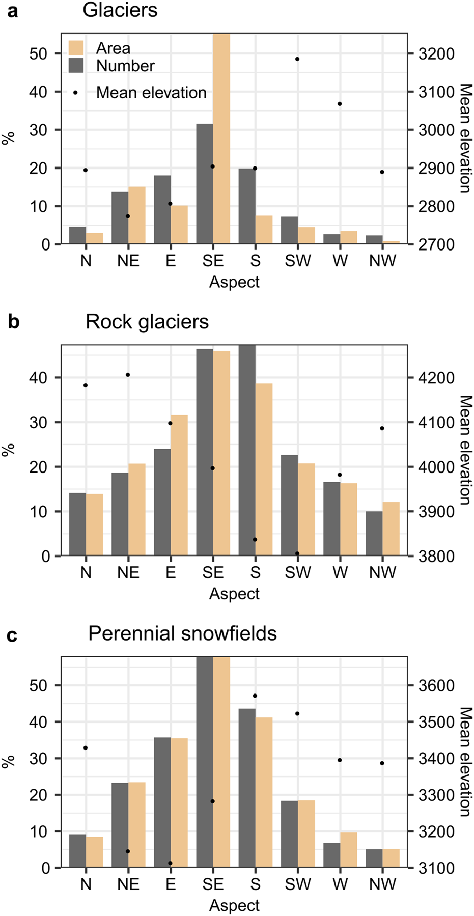
Fig. 7. Total area, number and mean elevation of ice masses classified according to their aspect.
The distribution of ice masses by elevation bands shows that the mean altitude decreases from ca. 5000 m a.s.l. in the north to ca. 1000 m a.s.l. in the south. In the Desert Andes, ice bodies are found at very high altitudes and the presence of several high peaks (some above 6000 m a.s.l.) along the Cordillera Oriental, located to the east, allows the existence of ice masses up to 65° W, the easternmost position of ice masses in Argentina and South America. To the south, starting in the Central Andes, ice masses are grouped along a narrower Cordillera fringe, within a wider range of elevation from 2700 to 6900 m a.s.l. In the Northern Patagonia Andes, ice masses are situated at lower altitudes from 1000 to 4600 m a.s.l. and at even lower elevations in the Southern Patagonia Andes from 200 up to 3500 m a.s.l. In Tierra del Fuego Andes ice masses are distributed between ~500 and 1450 m a.s.l. (Fig. 8).
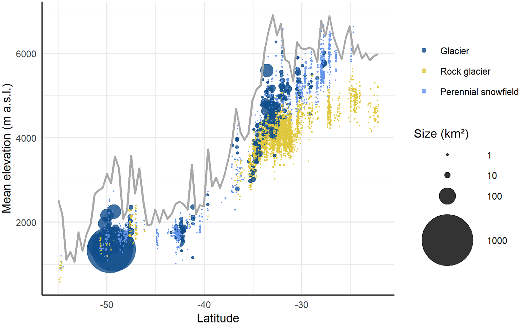
Fig. 8. Distribution of the ice mass sizes, elevation and latitude in the Argentinean Andes. Ice mass types are shown in different colors and size (circle diameter according to the logarithm of the glacierized area). The grey line at the background represents the maximum elevation profile of the Andes.
5.2. Ice mass distribution along the Argentinean Andes
Ice masses are found along the whole extension of the Argentine Andes. However, the distribution varies not only with latitude but also in cross-barrier direction.
The first glacier in the form of mountain glacier appears at ~25° S and valley glaciers and glaciers with debris-covered ice are located to the south of 29° S. The area covered by glaciers increases noticeably towards the south in the Central Andes, mainly between 31° S and 33° S. Glaciers in this region show large extents covered by debris; almost 70% of all glaciers are partly debris-covered and represent ~20% of the whole glacierized surface in this area. This is one of the areas with the highest percentage of glaciers with debris-covered ice in the world (Scherler and others, Reference Scherler, Wulf and Gorelick2018). A distinctive feature of this region is the great diversity of glaciers. In many cases, and especially in the larger bodies, complex geoforms can be found with the upper portions dominated by clean ice that gradually turns into debris-covered ice and rock glaciers at lower elevations. This mixed category here termed ‘debris-covered ice with rock glacier’ equals 15% of the entire inventoried area in the Central Andes. The Northern Patagonia Andes is characterized by a comparatively lower number of glaciers than farther north and dominance of mountain glaciers with the highest concentration of ice masses ~42° S. Southern Patagonia shows also a great diversity of glaciers, including the large SPI outlet glaciers in the west, the increasingly smaller valley and mountain glaciers to the east. The Andes in the Argentinean portion of Tierra del Fuego support many small mountain glaciers (<1 km2), mainly found on the highest peaks over 1000 m a.s.l. (Fig. 9a).

Fig. 9. Spatial distribution of ice masses in the different regions of the Argentinean Andes.
Rock glaciers constitute the only ice mass which is present all along the Argentinean Andes and are usually located at lower elevations than perennial snowfields, mountain and valley glaciers. In the Desert Andes, only rock glaciers are recorded at the northern end, between 22° S and 24° S. Within this region, the wetter eastern side shows a higher number and larger units compared to the drier western slopes, where the number of rock glaciers drops drastically to ~100 units over a study area of 55 000 km2. To the south, in the Central Andes, rock glaciers are larger than in the Desert Andes, with the largest rock glacier of the Argentinean Andes (just over 2 km2 in size) located at ~32° S. This region concentrates the highest number and area of rock glaciers in the Southern Andes, even superior to the Central Andes of Chile (Barcaza and others, Reference Barcaza2017). On the contrary, in Northern and Southern Patagonia few rock glaciers are found, they sum to 3% of the total number of units and 4% of the whole area with rock glaciers of the Argentine Andes. In Tierra del Fuego Andes rock glaciers constitute the second most numerous category and also the second in terms of the area covered (Fig. 9b).
Perennial snowfields are registered south of 24° S, and are regularly distributed in all regions along the Andes. They are also very numerous and small; none of them are >2 km2 in size (Fig 9c).
5.3. Fieldwork and uncertainty assessment
The mapping process of the NGI was validated through 40 field campaigns conducted along all the Andean regions between February 2012 and December 2017. The time invested in these trips represents a total of almost a year in the field, which allowed direct in situ measurements to be made for 1841 ice masses. We found a 95% agreement between the glaciers that were mapped and those that were observed in the field. For the clean-ice glaciers in Southern Patagonia, the agreement reached 98% while the Desert and the Central Andes, with a larger proportion of smaller glaciers, higher percentages of rock glaciers and glaciers with different degree of debris-covered ice, the agreement level was ~94%. Regarding the glacier classification (according to the operational categories), the agreement was ~91% for the entire Andes, with the Central Andes showing the lowest coincidence (85%). The main source of error detected in the field campaigns was related to the differentiation of active vs inactive rock glaciers. For the validation of the outline delineation, the outlines derived from satellite images were compared to direct field observations. Corrections in areas performed after the fieldwork amount to ~0.4% and are mainly associated with difficulties in interpreting the terminus of debris-covered ice and certain sectors of rock glaciers (Fig. S3).
The results of the digitization exercise of the glaciers mapped by six analysts show that the mean std dev. of the outlines is ~4% (for clean ice this value drops to 3%). As expected, the highest differences in the outlines were found in debris-covered and cast shadow areas. In the case of rock glaciers, the differences in the outlines are higher than in the case of clean ice glaciers, with a mean std dev. of 15% for all the units. We found that the mapping of the front of the rock glaciers was highly consistent but the upper parts showed greater differences depending on the analyst. Nonetheless, the difference between the mean area of rock glaciers obtained by the six analysts and the official outlines published in the NGI is −0.05%. In the case of glaciers, this difference is 3% (Table S2).
5.4. Regional glacier inventories vs global inventories (RGI)
Prior to the completion of the NGI, standardized information about glaciers in Argentina was only available from global datasets such as the RGI (RGI Consortium, 2017). A first comparison between the NGI and the latest version of the RGI (version 6.0) shows that local and regional inventories such as the NGI offer promising perspectives for improving the global products. For example, in the NGI there are 3800 (~45%) more glaciers than in the RGI, and this calculation is made without including the rock glaciers identified in the NGI. The inclusion of rock glaciers, partially debris-covered glaciers and many perennial snowfields allowed incorporation of 17 sub-basins that were not considered in the RGI, mostly in the Desert Andes and Central Andes where the arid to semi-arid conditions make these ice masses highly relevant as water resources. Mining activities are also largely located in these regions, and thus the detailed mapping of different ice masses, especially rock glaciers and debris-covered ice, allow more effective and efficient implementation of protection and conservation policies (Azócar and Brenning, Reference Azócar and Brenning2008).
The RGI 6.0 indicates that in the Southern Andes there are between 15 950 and 21 600 ice masses (lower or upper bounds of small ice masses), whereas in the SA the total number of ice bodies, without including rock glaciers, is 29 700 (and ~40 000 if rock glaciers are included). This represents a difference of −46 to −27% (depending if the lower or upper bound of small ice masses is used) in the number of ice masses between the RGI and SA (Fig. 10a). It is also worth noting that the largest discrepancy occurs in the number of small ice masses (<0.5 km2), which represent by far the majority of units in the Southern Andes. In this case, the RGI 6.0 has −53 to −32% less small ice masses than the SA. On the contrary, the difference in the number of ice masses >0.5 km2 is <5%. Regarding the total area covered by ice masses, the RGI 6.0 reports a glacierized area that is ~3% larger than the SA (without rock glaciers). Again, the difference between the datasets is higher for the smaller ice masses (−26 and −24% for the lower or upper bounds in the RGI) (Fig. 10b).
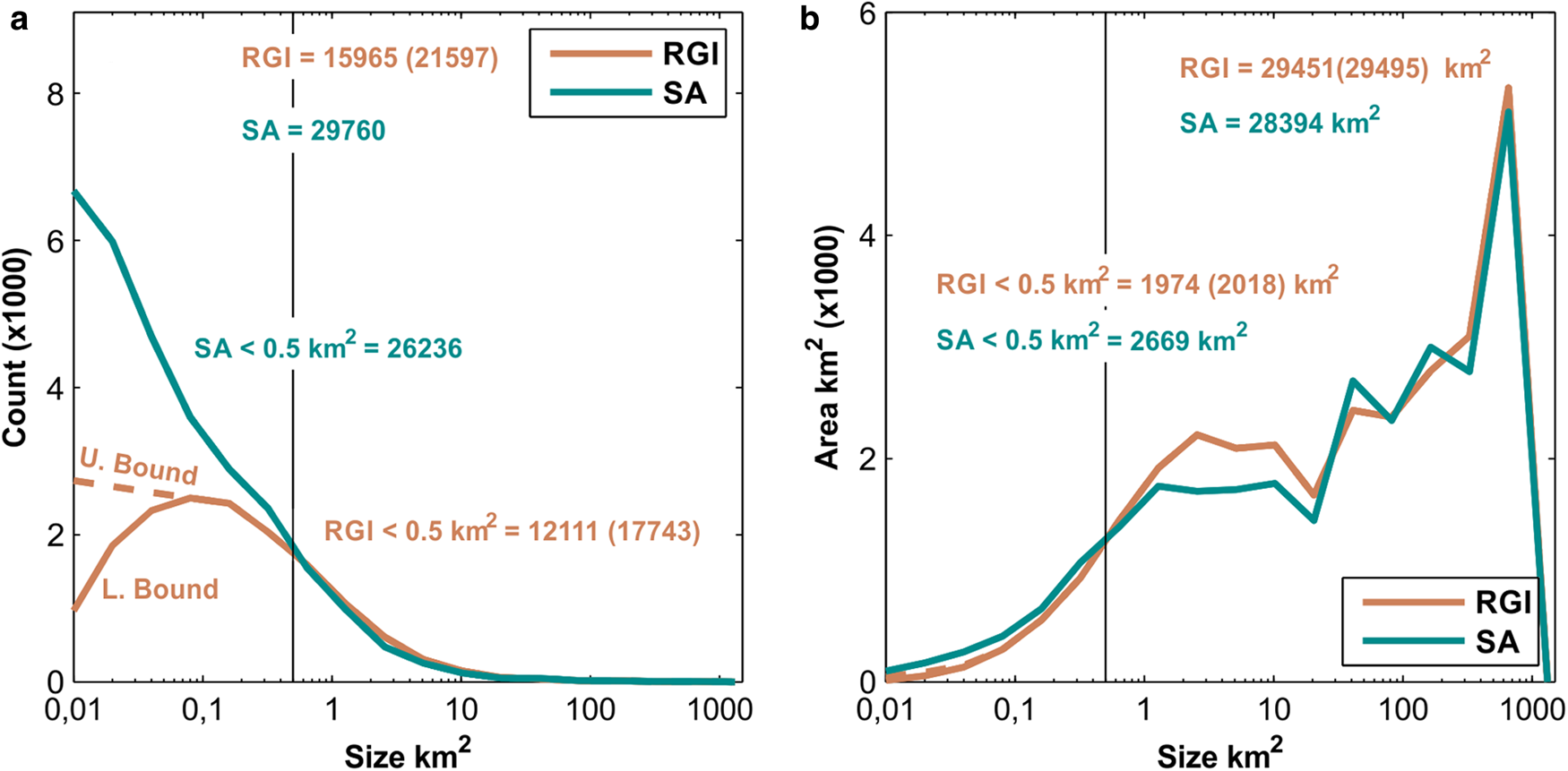
Fig. 10. (a) Number of ice masses for different unit sizes in the SA and the RGI 6.0. For the RGI 6.0, both the lower and upper bounds for ice masses <0.5 km2 are shown. (b) Same as (a) but for glacierized area vs unit size. The total area of ice masses in each inventory and the area of ‘smaller ice masses’ are also indicated. In both plots, the thin black vertical line indicates the boundary for ‘smaller ice masses’ (<0.5 km2). The number and extent of ice masses for the RGI 6.0 when the upper bound for smaller ice masses is used is shown in brackets.
In general, the RGI 6.0 and the SA show similar latitudinal patterns in terms of the number, extent and volume of ice masses. However, the total volume of glacier ice estimated for the RGI 6.0 is 16% smaller and for the SA. The disagreement with the RGI increases to −44% if we consider the volume of small glaciers alone, probably because of the larger number of small glaciers present in the SA inventory. Strong local discrepancies can also be observed between these datasets (Fig. 11). Clustering the data into one-degree latitudinal bands (Fig. 11a), it becomes evident that the number of ice masses in the RGI 6.0 is largely underestimated (with values ranging from −100 to −40% for most of the Southern Andes). In the Northern Patagonian Andes, in contrast, the RGI overestimates the number of glaciers by >150%. The smallest discrepancies between these datasets are observed in the Tierra del Fuego Andes, where the difference is below 10%. In terms of surface area covered by ice, in the Southern Patagonian Andes the difference is under 7%, showing that the largest ice masses (Southern Patagonian and Northern Patagonian Ice Fields) are well represented in the RGI 6.0. However, in the Desert Andes, where small ice masses prevail, the differences between the datasets range between −100 and +100% (Fig. 11b). In the North Patagonian Andes a large overestimation of >100% is observed in the RGI. In general, there is an underestimation in the volume of glacier ice in the RGI along the Southern Andes, with differences reaching up to −100% in the Desert Andes (Fig. 11c). Along the Central Andes we found −50% of underestimation in the ice volume in the RGI due to the lower number of ice masses in this dataset compared to the SA. Farther south, in the North Patagonian Andes the RGI shows an overestimation (more than 120%) in the volume of ice, but this large difference decreases to ~13% in the Southern Patagonian Andes.

Fig. 11. Number of ice masses (a), area (b) and volume (c) by one-degree latitude band along the Southern Andes for the SA and the RGI 6.0. The lines show the latitudinal totals and the bars show the differences between both datasets.
6. Discussion
6.1. Importance of the NGI
Argentina is one of the few countries with several thousand square kilometers of glaciers and ice-rich mountain permafrost features in its territory. However, despite the great number and surface area of ice masses and their undisputed socio-economic, hydrological, geopolitical, environmental and scientific-academic relevance, so far only a handful of glaciers have been studied in detail, and no information existed on the location, area and main characteristics of many ice masses. For example, we document the existence of rock glaciers of various sizes from 22° S in the Desert Andes up to 55° S in Tierra del Fuego, with a remarkable concentration in the Argentinean Central Andes ~ 31–34° S. This is particularly important as rock glaciers, which have received little attention in global inventories (due to a lack of freely available imagery with resolution of 10 m or higher, up until recently), are increasingly being considered as significant water sources that are more resilient than clean-ice glaciers and perennial snowfields to climate changes (Jones and others, Reference Jones, Harrison, Anderson and Whalley2019). Additionally, the applied methodology in rock glaciers delineation and characterization may represent a contribution to the IPA action Group Rock glacier inventories and kinematics which is currently working in establishing standard guidelines for inventorying rock glaciers (Delaloye and others, Reference Delaloye2018).
According to the Law, periodic updates should be conducted to evaluate changes in ice state across the Andes. Only minor changes are expected in debris-covered ice and rock glaciers in the near future inventories; however, the elevated rates of retreat documented in recent decades for clean ice masses, suggest major changes in perennial snowfields, small glaciers and low-elevation lying calving glaciers as those surveyed by the SPI (Sakakibara and Sugiyama, Reference Sakakibara and Sugiyama2014; Malmros and others, Reference Malmros, Mernild, Wilson, Yde and Fensholt2016; Barcaza and others, Reference Barcaza2017; Jones and others, Reference Jones, Harrison, Anderson and Betts2018; Braun and others, Reference Braun2019; Dussaillant and others, Reference Dussaillant2019; Leigh and others, Reference Leigh2019; Zemp and others, Reference Zemp2019).
Ice masses’ characteristics and their spatial distribution in Argentine Andes rely not only on the evident dependence of changing climates with latitude but also in cross-barrier direction. The interaction between the orography of the Andes and the atmospheric circulation induces contrasting climates at both sides of the Andes (Viale and others, Reference Viale2019). From local to regional scales, the Andean topography strongly controls the gradients of temperature and precipitation in the cross-barrier direction, which in turn also modulate ice mass types and their spatial distribution.
6.2. Differences between the glacier inventories of Argentina and Chile and the RGI 6.0
The comparison of the SA glacier inventory and the RGI 6.0 revealed several interesting findings. Although both datasets show overall similar values in terms of the total extent of ice masses, the RGI 6.0 shows a lower number and surface area of the smallest units, and an overestimation of the area covered by the largest glaciers (Fig. 10). When used for calculating, for example, the hydrological role of ice masses in a river basin where only small units are present, the importance of these glaciers as water resources will be obviously underestimated. On the contrary, for some basins in the Desert Andes where only rock glaciers are present, the inclusion of seasonal snow patches as perennial ice masses in the RGI 6.0 may overestimate the role of these ice masses as water resources. In the Southern Patagonian Andes, the differences in the extent and the number of ice masses between the SA and RGI are the lowest for the Southern Andes. Given that this region contains the bulk of the glacier ice in southern South America, these similarities provide independent validation for the assessment of the total ice volume and the recent and future contribution to sea-level rise of the entire Southern Andes region (Dussaillant and others, Reference Dussaillant2019; Farinotti and others, Reference Farinotti2019; Zemp and others, Reference Zemp2019).
7. Conclusions
For the first time, Argentina has a complete, detailed and standardized inventory, which includes 16 078 ice masses covering a total area of 5769 km2. This work constitutes original and unprecedented progress for glaciological, cryospheric, hydrological, climatological and many other related studies in Argentina. The inventory includes detailed maps and metadata of glaciers but also perennial snowfields and rock glaciers which show strong regional variations in their number, altitudinal distribution and surface area along the Andes. The inventory work also involved numerous field campaigns (~40) to validate the glacier maps and check the main characteristics and current status of many glaciers in the country. These campaigns also served to collect a valuable and very extensive photographic and cartographic database of many unexplored or poorly known areas of the Argentinean Andes. Compared to global inventories (RGI 6.0), the NGI provides more detailed information to protect the strategic water reservoirs in solid-state according to the mandates of the Argentinean legislation. Without the NGI many areas with ice masses in the Argentinean Andes would remain unknown, and consequently unprotected, particularly in arid to semi-arid regions which are highly sensitive to water scarcity. For the first time, any interested user can access, free of charge, accurate and updated information on the location, surface area, morphology and many basic physical parameters of all the frozen water reserves in the country. The use of a reliable and consistent methodology makes the results directly comparable among river basins, provinces and regions, and provides a very large and valuable cryospheric dataset with multiple uses at public and private levels. In particular, this new information can be of great help in the planning and management of water resources in arid to semi-arid Andean river basins. The new inventory can also help to improve the existing global inventories by providing more detailed information regarding the existence and actual boundaries of the different types of ice masses, especially in regions such as the Desert and Central Andes where rock glaciers and debris-covered ice are common but not always well defined in the global maps.
Supplementary material
The supplementary material for this article can be found at https://doi.org/10.1017/jog.2020.55
Data
The current NGI datasets are freely available and can be accessed at http://www.glaciaresargentinos.gob.ar and from the GLIMS database at http://www.glims.org/. Future updates of the NGI will be published periodically on these sites.
Acknowledgements
This work was supported by IANIGLA-CONICET and the Ministry of Environment and Sustainable Development. The satellite images were provided by the National Commission of Space Activities (CONAE for its initials in Spanish), GLIMS and the Japan International Cooperation Agency (JICA). We are very grateful to all who provided us support to conduct fieldwork all along the Andes such as the administrations of national and provincial parks, National Gendarmerie and Army, local authorities and communities. We are also very grateful to the National Geographic Institute (ING for its initials in Spanish), to past and present staff members of the National Glacier Inventory and to external collaborators. Finally, we thank the two reviewers and the Scientific Editor for their valuable and helpful comments.


 Open access