


1. Introduction
The response of the variation in Antarctic sea ice to global climate change has attracted increasing attention in recent decades. However, researchers still struggle to understand the mechanism responsible for the variation in Antarctic sea ice at the interannual scale, and current climate models exhibit an unsatisfactory performance when simulating Antarctic sea-ice variations (Turner and Comiso, Reference Turner and Comiso2017; Shu and others, Reference Shu2020). As an important component of the Antarctic climate system, landfast sea ice accounts for 35% (5%) of the total Antarctic sea-ice extent in summer (winter) (Fraser and others, Reference Fraser, Massom, Michael, Galton-Fenzi and Lieser2012). In East Antarctica, the contribution of landfast sea ice to the sea-ice mass balance is greater than the drifting sea ice (Giles and others, Reference Giles, Laxon and Ridout2008). The existence of landfast sea ice can reduce the energy exchange between the ocean and atmosphere, thereby affecting the regional atmospheric circulation and ecosystem.
Thermodynamic processes dominate the annual evolutionary cycle of landfast sea-ice thickness (h si) because of its immobility (Dumas and others, Reference Dumas, Carmack and Melliing2005). Accordingly, some previous studies have tested the sensitivity of the evolution of the Antarctic landfast sea-ice thickness to various thermodynamic processes using thermodynamic numerical models. For example, Heil and others (Reference Heil, Allison and Lytle1996) concluded that the sea-ice evolution is most sensitive to the oceanic heat flux, snow cover and albedo. In contrast, Yang and others (Reference Yang2016a) pointed out that the albedo is important in summer and that snow cover plays a minor role in Prydz Bay because of the effect of redistribution by wind. By comparing the evolution of first-year sea ice with that of second-year sea ice in a small scale (~10 km) landfast sea-ice zone, Zhao and others (Reference Zhao, Cheng, Yang, Vihma and Zhang2017) found that the conductive heat flux led to the differences in the evolution of first- and second-year sea ice because of the differences in sea-ice thickness. Nevertheless, although the sensitivities of some thermodynamic processes were tested in these studies by altering the corresponding parameterization scheme to force the model, evaluations of the parameterization schemes of thermodynamic processes remain limited due to the scarcity of observations, especially for the observations of turbulence and radiation fluxes over the sea ice; hence, the influence of the differences between parameterized and observed parameters on the simulation of sea-ice mass balance need to be better understood.
In particular, due to the sparsity of oceanic heat flux observations, the oceanic heat flux is the least documented parameter in thermodynamic studies of sea ice. In the Arctic, an oceanic heat flux of 2 W m−2 is widely considered a reasonable annual basin-averaged value during winter (Maykut and Untersteiner, Reference Maykut and Untersteiner1971). In Antarctica, reference values were obtained via model tuning with sea-ice thickness observations (Gordon and Huber, Reference Gordon and Huber1990; Heil and others, Reference Heil, Allison and Lytle1996; Lei and others, Reference Lei, Li, Cheng, Zhang and Heil2010; Yang and others, Reference Yang2016a; Zhao and others, Reference Zhao2019). Heil and others (Reference Heil, Allison and Lytle1996) suggested that the oceanic heat flux varied from 5 to 12 W m−2 within a full sea-ice season for the landfast sea ice off Mawson station. In Prydz Bay, East Antarctica, Lei and others (Reference Lei, Li, Cheng, Zhang and Heil2010) demonstrated that the oceanic heat flux derived based on the heat balance at the sea-ice bottom decreased from 11.8 W m−2 in April to 1.9 W m−2 in September; in contrast, Yang and others (Reference Yang2016a) reported that the oceanic heat flux decreased from 25 to 5 W m−2 during the growth season and recovered back to 25 W m−2 in summer. The oceanic heat flux shows a seasonal variation and some potential interannual changes. However, without sea-ice mass-balance measurements, it is difficult to quantitatively determine the oceanic heat flux, and thus, how to present a reasonable parameterization scheme for the oceanic heat flux in numerical models remains a topic of ongoing research.
Prydz Bay in East Antarctica is one of the local sites from which intensive observations have been acquired. There are four operational year-round stations within or surrounding Prydz Bay: Davis, Zhongshan, Progress II and Mawson, which makes the contribution of this region to the Antarctic landfast sea-ice monitoring network being particularly important. Previous studies concluded that the annual maximum first-year landfast sea-ice thickness ranged from 1.5 to 1.8 m and decreased to <1.0 m before break-up, while the maximum second-year landfast sea-ice thickness could even exceed 3 m in this region (Heil, Reference Heil2006; Tang and others, Reference Tang, Qin, Ren and Kang2006; Lei and others, Reference Lei, Li, Cheng, Zhang and Heil2010; Yang and others, Reference Yang2016a, Reference Yang2016b). In 2016, comprehensive observations were conducted over the landfast sea ice near Zhongshan station. High-quality datasets, especially turbulence fluxes over the sea ice, have been collected for the first time at this location (Liu and others, Reference Liu2020). These datasets provide an excellent opportunity to evaluate the thermodynamic parameterization schemes in numerical models.
Therefore, focusing on the thermodynamic processes of the landfast sea ice near Zhongshan station, this study aims to evaluate the thermodynamic parameterization schemes and further investigate the sensitivity of parameterization schemes to sea-ice thickness simulation in the sea-ice thermodynamic model. Furthermore, we attempt to identify a reasonable parameterization scheme for the oceanic heat flux. The data and methods are described in Section 2. Then, the results and discussion are presented in Section 3. Finally, the conclusions are given in Section 4.
2. Data and methods
2.1 Site and instruments
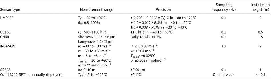
The observation site was located on landfast sea ice along the coast of Prydz Bay, East Antarctica, at 69°22′08.1″S 76°21′42.1″ E (Fig. 1a). During the observation campaign from 29 April to 31 October in 2016, a mast was put up on the sea ice to measure meteorological parameters (Hao and others, Reference Hao, Pirazzini, Yang, Tian and Liu2020). The instruments setup on the mast included (Fig. 1b): an HMP155 air temperature and humidity sensor (Vaisala Inc., Finland), a CS106 barometer (Vaisala Inc., Finland), a CNR4 net radiometer (Kipp & Zonen Inc., the Netherlands), an in situ, open-path, mid-infrared gas (CO2/H2O) analyzer integrated with a 3-D sonic anemometer (IRGASON, Campbell Sci. Inc., USA) and an SR50A sonic distance sensor used for snow depth (h s) measurement (Campbell Sci. Inc., USA). However, the SR50A sensor was broken after 1 September 2016, so the snow depth was measured manually once per day from then onward. Additionally, the cloudiness at Zhongshan station was observed visually every 6 h, the daily accumulated precipitation was measured at Russian Progress II station (located ~1 km from Zhongshan station), and the sea-ice thickness and sea-water temperature beneath the sea-ice bottom were recorded manually by borehole measurements about once a week, and the positions of measurements were very close to the observation site. The sea-water temperature was measured using a Cond 3210 SET1(Xylem Inc., Germany) sensor during the sea-ice thickness measurement. To derive one record of sea-ice thickness at least three repeat measurements were made, and these three measurements were made on the same core. The uncertainty of measured sea-ice thickness is ~±0.005 m. This is a low-end estimate of the sea-ice thickness uncertainty, which originates from the variability between cores. The key technical specifications and installation information of these instruments are summarized in Table 1. The meteorological data were first published in Liu and others (Reference Liu2020), and the data processing and quality control procedures were the same as those in Liu and others (Reference Liu2020), while the sea-ice data are first presented in this study. We consider the positive heat fluxes as the surface or sea-ice bottom gains the energy, while the negative heat fluxes indicate the surface or bottom loses energy in this study.

Fig. 1. (a) Geographical location of the observation site (red dot), (b) the local topography and (c) the meteorological tower at the observation site.
Table 1. Key technical specifications and installation information of the sensors
2.2 Sea-ice model
2.2.1 Model description and initial setup
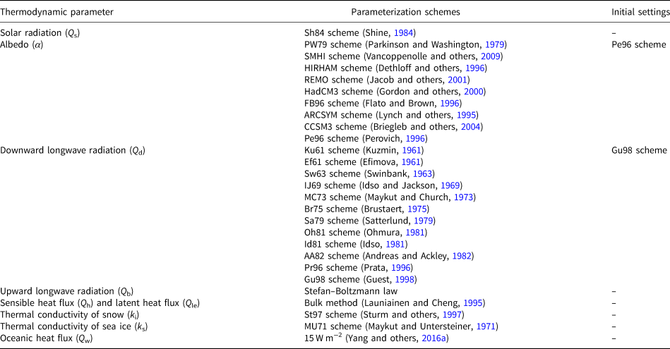
The growth and ablation of landfast sea ice are controlled mainly by thermodynamic processes (Williams and others, Reference Williams2014). Hence, in this study, to simulate the landfast sea-ice mass balance, we choose a vertical 1-D thermodynamic snow and sea-ice model, i.e. the high-resolution thermodynamic snow/ice (HIGHTSI) model (Launiainen and Cheng, Reference Launiainen and Cheng1998). To date, this model is widely used as a tool to investigate the influence of sea-ice properties or synoptic process on the simulation of sea-ice mass balance in the Antarctica and Arctic (Cheng and others, Reference Cheng, Mäkynen, Similä, Rontu and Vihma2013; Zhao and others, Reference Zhao, Cheng, Yang, Vihma and Zhang2017; Merkouriadi and others, Reference Merkouriadi, Cheng, Graham, Rösel and Granskog2017, Reference Merkouriadi, Cheng, Hudson and Granskog2020). The main thermodynamic processes and corresponding parameterization schemes, as well as their initial settings included in the HIGHTSI model are summarized in Table 2. Five input variables wind speed (U), air temperature (T a), relative humidity (R h), cloudiness (C n) and precipitation (P) were initially used to force the model. Note that HIGHTSI does not consider the effects of blowing snow on the snow depth, even though blowing snow may play an important role in local snow accumulation. Hence, to eliminate the uncertainty of the snow depth simulation, we use the observed snow depth instead of precipitation to force the model. The initial sea-ice thickness and snow depth input for modeling are 0.53 and 0.23 m, respectively, which are observed on 29 April 2016.
Table 2. Various parameterization schemes that can be used in the HIGHTSI model
As shown in Fig. 2a, the maximum 6 hourly averaged wind speed attains 13.7 m s−1, and the mean wind speed is 4.1 m s−1. The mean air temperature is −16.8°C, and the 6 hourly averaged maximum and minimum air temperatures are −1.6 and −47.1°C, respectively (Fig. 2b). For the surface temperature, which is derived from measured longwave radiation with the Stefan–Boltzmann relation (e.g. Vihma and others, Reference Vihma, Johansson and Launiainen2009; Yang and others, Reference Yang2016b), the mean value is −18.6°C. The 6 hourly averaged maximum and minimum surface temperatures are −3.8 and −47.8°C, respectively (Fig. 2b). The half-hourly averaged surface temperature is first observed to attain 0°C on 31 October. It is noted that the surface temperature refers to the surface skin temperature regardless of the bare sea-ice surface or snow surface. For the relative humidity (Fig. 2c), the mean value is 57.1%. Figure 2d shows the variation in cloudiness observed visually every 6 h. For the whole observation period, the proportions of C n ⩽ 0.1 and C n ⩾ 0.9 are 38.1 and 44.0%, respectively. Since the time step of the HIGHTSI model is set to 30 min in this study, we interpolate the observed cloudiness every 6 h in half-hour increments. Figure 2e describes the variation in snow depth. The snow depth is maintained at ~0.2 m before heavy precipitation occurred on 11 July, due to which the snow depth sharply increases to a maximum of 0.67 m; then, the snow depth gradually decreases until 15 August. From 1 September to 31 October, the accumulated snow shows a slight decreasing trend, and the snow depth attains 0.12 m at the end of the observation period. As shown in Fig. 2e, the precipitation is concentrated in June (25.0 mm) and July (44.1 mm), and the maximum daily precipitation of 19.2 mm occurred on 11 July.

Fig. 2. Time series of the observed 6 hourly averaged (a) wind speed, (b) air temperature, (c) relative humidity, (d) cloudiness, (e) snow depth and (f) daily precipitation during the whole observation period.
2.2.2 Design of controlled trials
To evaluate the parameterization schemes of different thermodynamic processes in the HIGHTSI model, we directly compare the results of solar radiation (Q s), albedo (α), downward longwave radiation (Q d), upward longwave radiation (Q b), sensible heat flux (Q h) and latent heat flux (Q le) from parameterization schemes with the corresponding observations. Then, we analyze the sensitivities of the simulation of sea-ice thickness to the differences between the parameterizations and observations through controlled trials. In the control groups, all the thermodynamic processes in the HIGHTSI model are described by parameterization schemes. In the experimental groups, we prescribe (rather than parameterizing) one variable using our observations to force the model. For example, to evaluate the influence of the differences between the parameterized and observed solar radiation on the sea-ice thickness simulation, we compare the simulation results from the HIGHTSI model forced by observed U, T a, R h, C n and h s (the control group) with those forced by observed U, T a, R h, C n, h s and Q s (the experimental group). Analogously, the design of the other control trials is described in Table 3. It should be noted that we use observed snow depth to force the model, the effects of thermodynamic processes on snow melting will be ignored, which may affect the reliability of sensitivity tests. However, during the sea-ice growth season the influence of thermodynamic processes on determining snow depth is negligible and the conclusion drawn from sensitivity studies by using observed snow depth will not be unreliable because of eliminating the feedback of thermodynamic processes on snow depth. In addition, to further understand the effects of the oceanic heat flux on the sea-ice thickness simulation, we compare the simulation results with different oceanic heat flux values, i.e. exp. F1 (Q w = 5 W m−2), exp. F2 (Q w = 15 W m−2) and exp. F3 (Q w = 25 W m−2). These values of Q w are in the typical range of Q w reported by previous studies in Antarctica (Gordon and Huber, Reference Gordon and Huber1990; Heil and others, Reference Heil, Allison and Lytle1996; Lei and others, Reference Lei, Li, Cheng, Zhang and Heil2010; Yang and others, Reference Yang2016a; Zhao and others, Reference Zhao2019).
Table 3. Design of the controlled trials

2.3 Calculations of sea-ice thickness in the HIGHTSI model
The total sea-ice thickness change is determined by the sea-ice evolution at the surface and bottom. At the surface, the melting dominated the change of snow or sea-ice thickness, and it can be expressed as (Launiainen and Cheng, Reference Launiainen and Cheng1998):

where Q m is the excess energy consider to melt the snow or sea ice when the surface temperature exceeds the melting point, ρ i is the sea-ice density, L f is the latent heat of freezing and (dh si/dt)sur is the snow or sea-ice thickness change at the surface.
At the sea-ice bottom, the sea-ice thickness change can be calculated as:

where (dh si/dt)bot is the sea-ice thickness change at the bottom, k i is the thermal conductivity of sea-ice, (∂T i/∂z)bot is the temperature gradient at the bottom and Q w is the oceanic heat flux. Finally, the total sea-ice thickness change (dh si/dt)tot can be derived according to:

2.4 Parameterizing the oceanic heat flux
In the HIGHTSI model, the ocean mixed-layer model is not included and the oceanic heat flux is set as a constant. However, some previous studies reported that the oceanic heat flux in the landfast sea-ice zone in Antarctica exhibited significant seasonal variation (Heil and others, Reference Heil, Allison and Lytle1996; Lei and others, Reference Lei, Li, Cheng, Zhang and Heil2010; Yang and others, Reference Yang2016a; Zhao and others, Reference Zhao2019). Hence, we consider presenting a modified parameterization scheme for the oceanic heat flux. The oceanic heat flux can be accurately expressed as:

where ρ s and c ps ( = 3980 J kg−1 K−1, Ackley and others, Reference Ackley, Xie and Tichenor2015) are the density and specific heat capacity of sea water respectively, and 〈w s'T os'〉 is the vertical turbulent heat flux of sea water, which can be obtained by using acoustic Doppler velocimetry combined with conductivity, temperature and depth measurements. However, we had not measured ocean turbulence or velocity below the sea ice. To obtain the Q w without turbulent measurements, McPhee and others (Reference McPhee, Kottmeier and Morison1999) used the bulk method to estimate 〈w s'T os'〉:

where C Hs is the bulk transfer coefficient for heat in the sea, and the reference value is 0.0057 (Kirillov and others, Reference Kirillov, Dmitrenko, Babb, Rysgaard and Barber2015); T os and T w are the sea-water temperature beneath the sea ice and the temperature of the sea-ice bottom, respectively, where T w is set as −1.8°C according to Heil and others (Reference Heil, Allison and Lytle1996); u 0* is the frictional velocity beneath the sea ice. For the landfast sea ice, the quadratic resistance law can be used to describe the relationship between u 0* and the velocity of sea water (U s) according to Jenkins and others (Reference Jenkins, Nicholls and Corr2010):

where c w is a dimensionless drag coefficient, and the reference value is 0.0055 (Hibler, Reference Hibler1979). Unfortunately, we lack the observations on U s. To simply optimize the oceanic heat flux without U s observations in the HIGHTSI model, we suppose that:

where k c is the empirical coefficient. As shown in Eqns (4–6), k c should be related to the current velocity, density and heat capacity of sea water. In this study, k c is assumed to be a constant. To determine the best possible value of k c, the HIGHTSI model is ran with a step of 0.1 W m−2 °C−1 within the range from 0 to 50 W m−2 °C−1 of k c. It should be noted that all the surface thermodynamic processes are prescribed based on the observations in these experiments. Then the optimal value of k c can be identified when the minimum bias between the modeled and observed sea-ice thicknesses is obtained. Hence, k c is a tuning parameter.
3. Results and discussion
3.1 Evaluation of the solar radiation parameterization scheme
In the HIGHTSI model, the Q s parameterization scheme for a clear sky was proposed by Shine (Reference Shine1984), and a cloudiness factor of (1 − 0.52C n) is used for cloudy conditions (Bennett, Reference Bennett1982). As shown in Fig. 3a, the parameterization scheme of Q s can accurately reproduce the observations during the period from May to September when the Q s is relatively small. However, the parameterized Q s is underestimated in some periods after September. This is partially caused by the uncertainty in the visually observed cloudiness because it is observed at Zhongshan station, ~1 km away from our sea-ice measurement site. In addition, the using of empirical cloudiness factor of (1 − 0.52C n) may be another cause for the underestimation of Q s, for example, the cloudiness factor of (1 − 0.6C n3) proposed by Parkinson and Washington (Reference Parkinson and Washington1979) produces larger solar radiation reaching to the surface when C n < 0.94. Figure 3b presents the observed and parameterized daily maximum Q s, revealing that the parameterized daily maximum Q s is underestimated after mid-October.

Fig. 3. Comparison of the (a) solar radiation and (b) daily maximum solar radiation between the observed (red line) and parameterized (black line) results, (c) the comparison among observed sea-ice thickness (blue dots), simulated sea-ice thickness by the parameterized solar radiation (black line) and that by the observed solar radiation (red line) and (d) the differences between the sea-ice thickness simulated by the parameterized solar radiation and that simulated by the observed solar radiation.
To quantitatively understand the influence of the differences between the parameterized and observed Q s on the sea-ice thickness simulation, Fig. 3c compares the sea-ice thickness simulated by the parameterized Q s with that simulated by the observed Q s, which the results demonstrate are very similar to each other. As shown in Fig. 3d, the relative difference, defined as the ratio of the difference between the sea-ice thickness simulated by the parameterized Q s and that simulated by the observed Q s to the sea-ice thickness simulated by the observed Q s (a similar definition is used for the following variables), is <0.1% before October but increases to a maximum of 0.36% at the end of October. While the absolute difference, defined as the sea-ice thickness simulated by the parameterized Q s minus the sea-ice thickness simulated by the observed Q s (a similar definition is used for the following variables), does not exceed 6 × 10⁻³ m during the whole observation period. These results indicate that the effects of the differences between the parameterized Q s and observed Q s on the sea-ice thickness simulation are negligible in the HIGHTSI model during the observation period.
Figure 3c also presents the observed sea-ice thicknesses obtained by borehole measurements. The observed sea-ice thickness is 0.53 m at the beginning of the observation period and gradually grows to a maximum of 1.82 m by 18 October 2016. Comparing with the simulated sea-ice thickness by the HIGHTSI model under initial settings (equivalent to the sea-ice thickness simulated by the parameterized Q s), it is clear that the simulation results are consistent with observations before mid-June, but they are significantly underestimated after mid-June. The differences between the simulation results and observations tend to increase with time.
3.2 Evaluation of albedo parameterization schemes
There are nine parameterization schemes for α in the HIGHTSI model (as shown in Table 2). Figure 4a presents the parameterized α and the observed monthly mean α when the observed daily maximum Q s > 20 W m−2. The std dev. of observed monthly mean albedo is ~0.06 for each month. According to the variation in the observed monthly mean α, the maximum of 0.86 appears before August 2016, and the observed monthly mean α gradually decreases from July to October, which is related to the metamorphism of the snow cover. Moreover, the parameterization result of 0.86 from the REMO scheme is more consistent with the observations before August compared with those from the other schemes; however, in August and September, the Pe96 scheme and SMHI scheme perform better, respectively, and the HadCM3 scheme performs better than the other schemes in October. Generally, the current version of the HIGHTSI model cannot accurately describe the seasonal variation in α over snow surface by using a single parameterization scheme.

Fig. 4. Comparison of albedo between the observed and parameterized results, and (b) the relative differences and (c) absolute differences in the sea-ice thickness simulated using various albedo parameterization schemes against that simulated using the observed albedo.
Furthermore, we examine the influence of the parameterized α on the sea-ice thickness simulation. Figures 4b, c present the relative differences and the absolute differences in the sea-ice thickness simulated using different α parameterization schemes compared with that simulated using the observed α. The relative differences of all parameterization schemes are small before September but show considerable diversity after September. The relative differences of the CCSM3 scheme maintain a continuous increase after September, and the increase is the largest among all the schemes, attaining 3.5% at the end of the observation period. In contrast, the relative differences of the HadCM3 scheme are maintained at <0.3% during the whole observation period, indicating that the HadCM3 scheme is the best choice for parameterizing α in the HIGHTSI model. It can also be found that the PW79, HIRHAM, HadCM3, FB96, ARCSYM and CCSM3 schemes produce negative absolute differences after September, while the absolute differences of SHMI, Perovich and REMO schemes are positive. In addition, Yang and others (Reference Yang2016a) concluded that the simulation of sea-ice thickness is very sensitive to the setting of the α parameterization scheme in the HIGHTSI model during the melting season. However, our results show relatively low sensitivity of the sea-ice thickness simulation to the α parameterization scheme because our experiment is carried out mainly during the growth season of sea ice, when Q s is relatively small.
3.3 Evaluation of the longwave radiation parameterization schemes
The longwave radiation budget plays an important role in the surface heat balance, especially during winter when the shortwave radiation is relatively weak. However, the inaccuracy in estimating the atmospheric longwave radiation Q d even under clear-sky conditions tends to be considerable (Launiainen and Cheng, Reference Launiainen and Cheng1998). In the HIGHTSI model, there are 12 parameterization schemes for determining Q d. The cloudiness factor of (1 + 0.26Cn) is used for cloudy conditions in Ef61, Sw63, Br75, Oh81, Id81, AA82, Pr96 and Gu97 schemes (Jacobs, Reference Jacobs1978), and the cloudiness factors of (1 + 0.12C n), (1 + 0.275C n), (1 + 0.2232C n2.75) and (1 + 0.2C n2) are used in Ku61, IJ69, MC73 and Sa79 schemes, respectively. Figure 5 compares the observed Q d and parameterized Q d obtained by these schemes. The bias, which is defined as |observedQ d − parameterizedQ d|/m (m is the number of samples), reflects the absolute difference between observations and parameterizations. Our results show that the Pr96 scheme produces the smallest bias, but the bias from the Br75 scheme is the largest. To evaluate the consistency of variation, the correlation coefficient (R) is also given in Fig. 5. It is found that the parameterizations based on the Ef61, IJ69, Br75, Id81, AA82 and Pr96 schemes show the highest correlation with observations, while the Ku61 scheme performs the worst. In addition, the slope is also used to quantify the systematic deviation. It can be found that the parameterizations from the Br75 scheme show the most significant underestimation, and the parameterizations from the Id85 scheme produce the smallest systematic deviation. By using the observations collected in the Arctic, Key and others (Reference Key, Silcox and Stone1996) also evaluated some Q d parameterization schemes. They pointed that the Ef61 scheme for clear sky and the MC73 scheme for all-sky performed well, but AA82 scheme was less accurate for clear sky. Similar results can also be reproduced in our assessment.
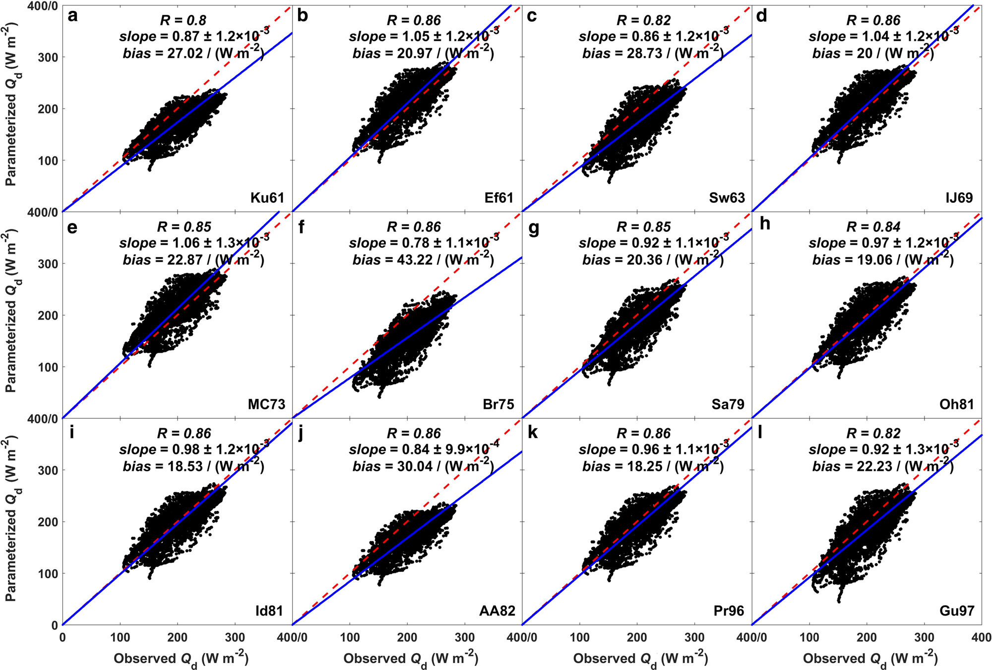
Fig. 5. Comparison between the observed atmospheric longwave radiation and parameterized atmospheric longwave radiation obtained using 12 different schemes. The red dotted line is the 1 : 1 line, and the blue solid line is the linear best-fitting line.
To further understand the influence of the differences between observed Q d and parameterized Q d on the sea-ice thickness simulation, Fig. 6 presents the relative differences in the sea-ice thicknesses simulated using various Q d parameterization schemes against that simulated using the observed Q d. As shown in Fig. 6a, the relative differences of the Id81 scheme are the smallest with an average of 0.5% during the whole observation period, whereas the relative differences derived from the Br75 scheme attain the maximum of 12.8%, and the average relative difference of the Br75 scheme (9.9%) is significantly higher than that of the other schemes. In addition, the Ef61, IJ69 and MC73 schemes present the negative absolute differences, while other schemes show the positive absolute differences. The Br75 (MC73) scheme produces the maximum positive (negative) absolute difference of 0.167 (−0.066) m at the end of the observation period. These results indicate that the choice of the Q d parameterization scheme is important when simulating the sea-ice thickness in the HIGHTSI model, and the Id81 scheme appears to be more applicable for the landfast sea ice in the coastal region of East Antarctica.

Fig. 6. (a) Relative differences and (b) absolute differences in the sea-ice thickness simulated using various atmospheric longwave radiation parameterization schemes against that simulated using the observed atmospheric longwave radiation.
The longwave radiation emitted from the snow/ice surface is determined using the Stefan–Boltzmann relation. In the HIGHTSI model, the surface temperature (T s) is described by the surface heat balance equation:

where F(T s) is the net flux, the term I 0 is the penetration part of solar radiation, and Q c is the conductive heat flux. Under freezing conditions, F(T s) should be equal to 0 W m−2. Then Eqn (8) can be solved effectively by the Newton iteration method (e.g. Launiainen and Cheng, Reference Launiainen and Cheng1998: refer to the HIGHTSI technical paper):

where ${F}^{\prime}( T_{\rm s}^n )$ denotes the derivative term with respect to T s. $T_{\rm s}^0$
 is the first guess of T s, which is set as T a − 0.5°C. Then, the iterative processes are made to match $\vert {T_{\rm s}^{n + 1} -T_{\rm s}^n } \vert < 0.01$
 , and the maximum iterative step is set to be 15 (i.e. n = 15). Once the value of T s is obtained, the corresponding Q b can also be derived by the Stefan–Boltzmann relation. Figure 7 compares the calculated Q b with the observed Q b, demonstrating that the calculated Q b is fractionally underestimated compared with the observed Q b. The bias, R and slope between the calculated Q b and observed Q b are 13.5 W m−2, 0.82 and 0.98, respectively.

Fig. 7. Comparison between the observed upward longwave radiation and calculated upward longwave radiation. The red dotted line is the 1 : 1 line, and the blue solid line is the linear best-fitting line.
On the other hand, the observed Q b can be used as an input to force the HIGHTSI model; in this case, the term related to Q b in F′(T s) should be eliminated. Figure 8 compares the sea-ice thickness simulated using the parameterized Q b against that simulated using the observed Q b, revealing that the former is generally larger than the latter, and the differences between them gradually increase during the sea-ice growth season. The mean relative difference (absolute difference) during the whole observation period is 5.4% (0.06 m), and the maximum relative difference (absolute difference) can attain 7.5% (0.09 m). In the HIGHTSI model, T s plays an important role in simulating sea-ice thickness because it not only determines the surface melting but also directly affects the snow and sea-ice temperature profiles. Although the surface melting can be ignored during the sea-ice growth season, the impacts of surface temperature on snow and sea-ice temperature profiles cause the differences of simulated sea-ice thickness by different parameterization schemes. The differences between parameterized Q b and observed Q b produce the relatively large differences in the calculated surface temperature, which further lead to the relatively large differences in the simulated sea-ice thickness. Furthermore, our results also show that the simulated sea-ice thickness is sensitive to the differences between parameterized Q b and observed Q b at the upper sea-ice boundary. This may indicate that the using of observed Q b instead of parameterized Q b induces the significant influence on the calculation of surface temperature.

Fig. 8. (a) Sea-ice thickness simulated using the parameterized upward longwave radiation (black line) and that simulated using the observed upward longwave radiation (red line) and (b) their relative (green line, scaled to the left y axis) and absolute (blue line, scaled to the right y axis) differences.
3.4 Evaluation of the turbulent heat flux parameterization schemes
In the HIGHTSI model, Q h and Q le are parameterized using the familiar bulk formula based on the Monin–Obukhov similarity (MOS) theory; the details of the calculation can be found in Launiainen and Cheng (Reference Launiainen and Cheng1998). The settings of the aerodynamic roughness length (z 0m) and scalar roughness length for temperature (z 0h) in the HIGHTSI model follow Banke and others (Reference Banke, Smith, Anderson and Pritchard1980) and Andreas (Reference Andreas1987). The z 0m calculated by Banke and others (Reference Banke, Smith, Anderson and Pritchard1980) is 1.42 × 10⁻⁴ m, and the z 0h ranges from 1.1 × 10⁻⁸ to 1.6 × 10⁻⁴ m according to Andreas (Reference Andreas1987). However, Liu and others (Reference Liu2020) analyzed the same dataset employed in this study and revealed that the values of z 0m and z 0h should be 1.9 × 10⁻³ and 3.7 × 10⁻⁵ m, respectively. Hence, the values of z 0m and z 0h in the HIGHTSI model are revised according to Liu and others (Reference Liu2020). Figures 9a, b compare the parameterized Q h and Q le against the corresponding observations, revealing that Q h is overestimated by the HIGHTSI model, whereas Q le is underestimated. The accuracies of the parameterized Q h and Q le are greatly inferior compared with the parameterization results of the radiation fluxes in the HIGHTSI model. For Q h, we further analyze why the parameterization result is markedly overvalued with the same z 0m and z 0h as employed by Liu and others (Reference Liu2020). We find that the underestimation of the calculated surface temperature in the HIGHTSI model is the main cause of the overvalued Q h. Thus, if we use the observed T s to calculate Q h with the same method as described in the HIGHTSI model, the parameterized Q h is consistent with the observations (as shown in Fig. 9c). For Q le, the inaccuracy may be related to the uncertainty in the surface humidity and the corresponding roughness length in the parameterization scheme. However, effective means with which to measure these key parameters are lacking. Hence, because of problems with identifying parameters and their availability, there is still an imperfection in parameterizing Q le within the MOS theory framework.
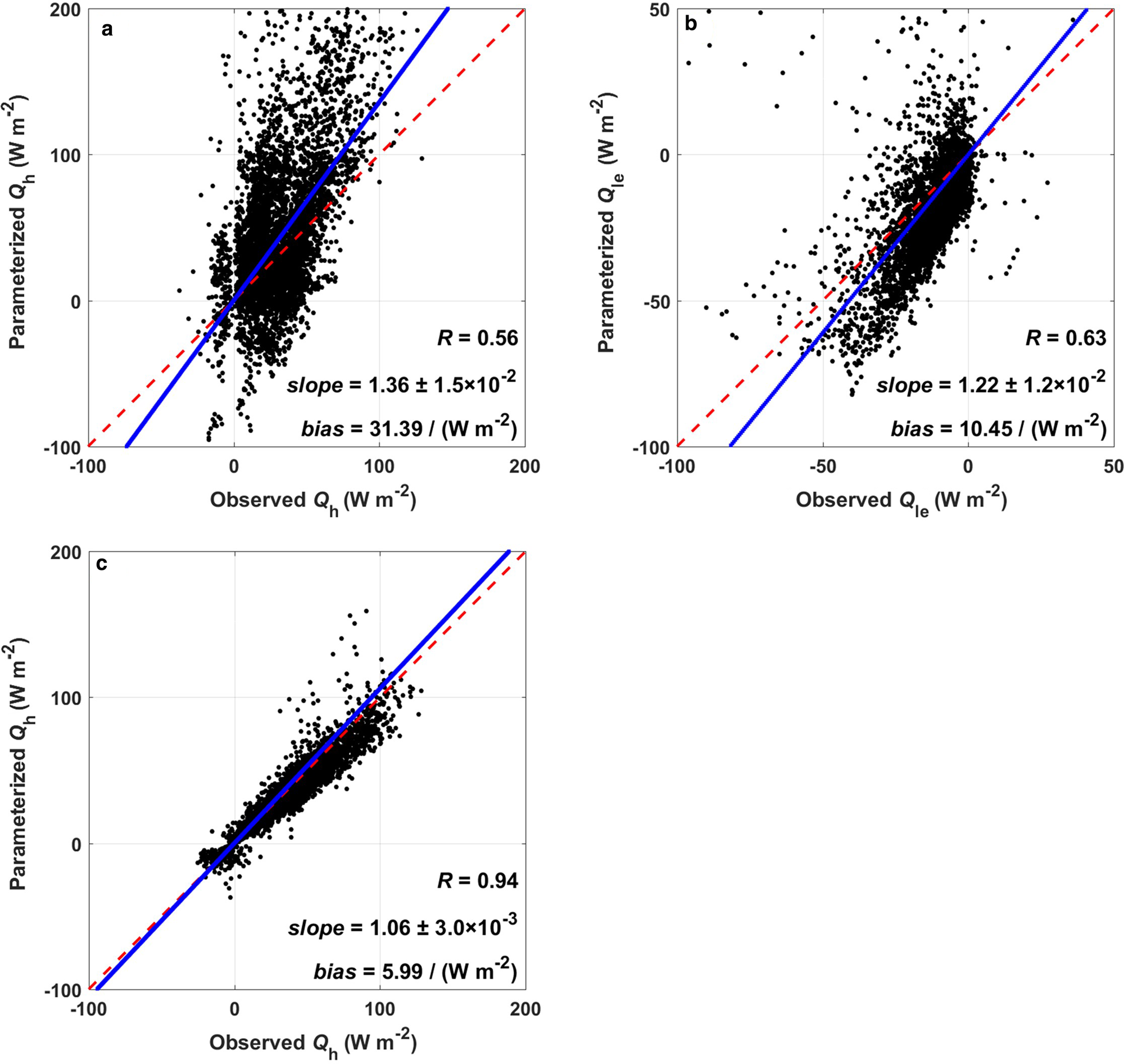
Fig. 9. Comparison of the parameterized (a) sensible heat flux and (b) latent heat flux in the HIGHTSI model with the corresponding observations, and (c) the comparison of the parameterized sensible heat flux by using observed surface temperature with observations.
Furthermore, to quantify the influence of the differences between the parameterized and observed surface turbulent heat fluxes (Q h and Q le) on the sea-ice thickness simulation, we compare the sea-ice thickness simulated by the parameterized Q h and Q le with that simulated by the observed Q h and Q le in Fig. 10, demonstrating that the latter is slightly thinner than the former. The maximum relative difference is only 5.5%, and the mean relative difference is 3.1%. For absolute differences, the maximum value of 0.05 m occurs in mid-July and mid-September and the mean absolute difference is 0.03 m. In addition, although the parameterized surface turbulent heat fluxes show a large discrepancy compared with observations, the influence of the differences between the parameterized and observed surface turbulent heat fluxes on the sea-ice simulation is smaller than that of the differences between the parameterized and observed Q b on the sea-ice simulation.

Fig. 10. (a) Sea-ice thickness simulated by the parameterized sensible heat flux and latent heat flux (black line) and that simulated by the observed sensible heat flux and latent heat flux (red line) and (b) their relative (green line, scaled to the left y axis) and absolute (blue line, scaled to the right y axis) differences.
3.5 Sensitivity test and improvement of the oceanic heat flux parameterization scheme
In the HIGHTSI model, Q w is initially set as a constant. However, Q w is highly dependent on the sea-water temperature, salinity and current velocity beneath the sea-ice bottom (Kirillov and others, Reference Kirillov, Dmitrenko, Babb, Rysgaard and Barber2015). Hence, a proper determination of Q w may necessitate coupling an ocean mixed-layer model. In the current study, we first test the sensitivity of Q w to the sea-ice thickness simulation during the growth season. Figure 11 shows the simulated sea-ice thicknesses obtained by exps. F1, F2 and F3. The simulated sea-ice thicknesses clearly vary with different values of Q w, and the differences tend to increase with time. The simulated maximum sea-ice thickness is 1.1 m when using Q w of 25 W m−2; however, it can attain 1.73 m when Q w is 5 W m−2. This result indicates that the sea-ice thickness simulation is very sensitive to Q w during the sea-ice growth season. Thus, it is crucial to accurately describe Q w in the HIGHTSI model.

Fig. 11. Simulated sea-ice thickness with the oceanic heat flux setting as 5 W m−2 (black line), 15 W m−2 (red line) and 25 W m−2 (blue line).
Furthermore, we derive a more reasonable Q w parameterization scheme by running the HIGHTSI model with the observed heat fluxes at the upper sea-ice boundary. As demonstrated in Section 2.4, a simple bulk formula is adopted to determine Q w. Figure 12a presents the observed T os − T w retrieved by borehole measurements, which are acquired at a frequency of approximately once a week. It should be noted that although the measurement depth of T os is not fixed, the sea-water temperature shows little variation with depth in the oceanic surface layer where the measurement of T os is conducted. To match the time step of 30 min for the model input, continuous daily T os − T w data are first generated through smoothing the observed T os − T w with moving average method. Then, the Q w scheme based on Eqn (7) is used to force the HIGHTSI model, and the value of k c in Eqn (7) is tested within the range from 0 to 50 W m−2 °C−1 with a step of 0.1 W m−2 °C−1. These experiments indicate the optimum k c of 21.8 W m−2 °C−1. Figure 12b exhibits the simulated sea-ice thickness by the model forced by measurements of U, T a, R h, C n and h s, plus measurements of all the upper interface fluxes when k c is set as 21.8 W m−2 °C−1. It can be found that the simulated sea-ice thickness is in good agreement with the observations, and the smallest mean bias of 0.05 m is obtained when k c is set as 21.8 W m−2 °C−1.

Fig. 12. (a) Observed T os − T w (red triangle) and smoothed result (red line), and (b) the observed sea-ice thickness (blue circle), simulated sea-ice thickness with k c = 21.8 W m−2 °C−1 (blue line), and the corresponding oceanic heat flux (black line) in 2016.
Figure 12b also shows the corresponding time series of Q w, which clearly exhibits a seasonal variation characterized by a decrease from 7.5 W m−2 at the beginning of the observation period to 0.9 W m−2 at the end. The seasonal variation of Q w reflects the seasonal variation of sea-water temperature, which is related to the water masses advected along the shelf (Heil and others, Reference Heil, Allison and Lytle1996). Some previous studies reported the similar Q w value to our results. For example, Heil and others (Reference Heil, Allison and Lytle1996) found that Q w was <2 W m−2 during the period from early July to late November in the Prydz Bay region; Lei and others (Reference Lei, Li, Cheng, Zhang and Heil2010) indicated that Q w decreased from 11.8 (±3.5) W m−2 in April to 1.9 (±2.4) W m−2 in September at Zhongshan station. However, some studies also show that Q w exits significant interannual and spatial variability (Heil and others, Reference Heil, Allison and Lytle1996; Perovich and Elder, Reference Perovich and Elder2002; Kirillov and others, Reference Kirillov, Dmitrenko, Babb, Rysgaard and Barber2015). In addition, a similar seasonal variation pattern of Q w was reported by Yang and others (Reference Yang2016a). However, although Yang and others (Reference Yang2016a) also used the HIGHTSI model combined with observed sea-ice thicknesses to derive Q w near Zhongshan station, they reported that Q w decreased from 20 to 5 W m−2 during the same season as our experiment. A possible explanation is that they used U, T a, R h, C n and P only to force the HIGHTSI model; that is, the thermodynamic processes at the upper boundary were parameterized. In contrast, in our study, to reduce the errors caused by parameterization schemes at the upper boundary, the observed surface energy fluxes are used to force the HIGHTSI model. Furthermore, by using surface temperature and sea-ice thickness observations to solve the thermal energy balance equation at the bottom of sea ice (named the heat residual method), Zhao and others (Reference Zhao2019) discovered that the monthly mean Q w in May was 27 W m−2 and fell to ~10 W m−2 after July. Compared with the method used in our study, the heat residual method is simpler; nevertheless, the heat residual method produces a periodic 1- to 2-month oscillation (Lei and others, Reference Lei, Li, Cheng, Zhang and Heil2010; Zhao and others, Reference Zhao2019). Hence, the heat residual method may be less reliable because it produces a spurious oscillation.
On the other hand, to verify the applicability of new Q w parameterization scheme, the U, T a, R h, C n and h s data collected at the same site during the period from 29 April to 31 October in 2017, and the calculated Q w by using the formula of k c × (T os − T w) with k c = 21.8 W m−2 °C−1 is used to force the HIGHTSI model. Due to the lack of reliable measurements of the upper interface fluxes in 2017, the thermodynamic processes are parameterized in the HIGHTSI model and the choices of parameterization schemes are based on our evaluation results. As shown in Fig. 13a, the calculated Q w decreases from 9.9 W m−2 at the beginning of observation period to the minimum of 1.5 W m−2 on 5 October 2017, and it shows a slight increase in trend after 5 October 2017. By using this calculated Q w to force the HIGHTSI model, the simulated sea-ice thickness shows good agreement with the observations, however, the simulated sea-ice thickness simulated by the constant Q w of 15 W m−2 is significantly underestimated compared with the observations (Fig. 13b). Hence, these results indicate that the new parameterization scheme of Q w is useful across two seasons at Prydz Bay. Compared with the calculated Q w in 2016, the calculated Q w in 2017 looks to be a different magnitude across both years by 25%, but the new parameterization scheme still works well. Furthermore, the best parameterization in 2016 also works well in 2017, which indicates the robustness of the new parameterization.

Fig. 13. (a) Observed (red triangle) and smoothed (red line) T os − T w, and the calculated oceanic heat flux Q w by k c × (T os − T w) with k c = 21.8 W m−2 °C−1 (black line), and (b) the comparison between observed sea-ice thickness (blue circle) and simulated sea-ice thickness with Q w = 15 W m−2 (blue line) and Q w = k c × (T os − T w) with k c = 21.8 W m−2 °C−1 (red line) in 2017.
It should be noted that our study presents a constant k c, however, as demonstrated in Section 2.4, k c should be related to the current velocity, which exists a daily variation (Jenkins and others, Reference Jenkins, Nicholls and Corr2010). In addition, the T w, which is set as a constant of −1.8°C in this study, should depend on the salinity of the underlying sea water (Vancoppenolle and others, Reference Vancoppenolle, Madec, Thomas and McDougall2019) and the settings of T w will also have impacts on k c. Hence, the representativeness of k c we presented may be limited to the local scale and the temporal variation characteristic of k c is lost. To develop a more realistic Q w parameterization scheme, the measurements of current velocity, salinity, as well as some turbulent parameters in the oceanic surface layer are still required.
3.6 Seasonal variation in the heat budget and its influence on the sea-ice thickness variation
The monthly mean net shortwave radiation Q s(1 − α) − I 0, net longwave radiation (Q d − Q b), Q h, Q le, Q c, F(T s), Q w and the monthly growth of sea-ice thickness are presented in Table 4. These values are calculated from the results of modeling experiment, which is driven by the observed surface heat fluxes and with best choice of K c. It can be found that the net shortwave radiation, Q h, and Q c are the heat sources at the snow surface, while the net longwave radiation and Q le are the heat sinks at the snow surface during the growth season. From May to September, the surface loses energy to atmosphere through radiation fluxes, mainly due to a negative net longwave radiation, while Q h and Q c become the leading heat source. The monthly mean Q w gradually decreases from 6.2 W m−2 in May to 1.2 W m−2 in October, and the value of the monthly mean Q w is small compared with the other terms. Among these heat budget terms, the seasonal variation in the net shortwave radiation is the most significant, increasing from 0 W m−2 in June to 39.8 W m−2 in October. It can also be found that the larger Q c and the smaller Q w will intensify the growth of the sea-ice bottom. For example, the Q w in August is similar to that in September, however, the Q c in August is 9.6 W m−2 m larger than that in September, which leads to the more sea-ice growth in August. In October, the significantly reduced Q c leads to the minimum of sea-ice growth. In addition, although the Q c in August is close to that in May, caused by the smaller Q w in August, the sea-ice growth in August is larger than that in May. Hence, this case indicates the smaller Q w is conducive to the growth of the sea ice. Table 4 also presents the monthly mean net flux, which is assumed to be equal to 0 W m−2 in the calculation of surface temperature. It is clear that the model results agree with the assumption of F(T s) = 0 W m−2 under freezing conditions.
Table 4. Monthly mean heat fluxes and sea-ice thickness from May to October and their std dev values as calculated from model tuning results.

4. Summary
By using data collected throughout the sea-ice growth season over the landfast sea ice in Prydz Bay, East Antarctica, the parameterization schemes of thermodynamic processes at the upper sea-ice boundary in the HIGHTSI model are examined, and we propose a modified oceanic heat flux (Q w) parameterization scheme.
Comparing the results of solar radiation (Q s), albedo (α), downward longwave radiation (Q d), upward longwave radiation (Q b), sensible heat flux (Q h) and latent heat flux (Q le) from the parameterization schemes with the corresponding observations reveals that the surface turbulent flux parameterization schemes produce the largest deviations from the observations. However, although the parameterized Q h and Q le present the largest deviations from the observations, the influence of this deviation on the sea-ice thickness simulation is not the most significant. At the upper sea-ice boundary, the differences between the parameterized and observed Q b tend to have the greatest influence on the simulated sea-ice thickness. In addition, our results suggest that the best choices for the α and Q d parameterization schemes in the HIGHTSI model are the HadCM3 scheme and Id81 scheme, respectively. Furthermore, the simulated sea-ice thickness is very sensitive to Q w during the sea-ice growth season. Hence, it is important to select a reasonable Q w parameterization scheme in the HIGHTSI model. In the current study, a modified scheme of k c × (T os − T w) with k c = 21.8 W m−2 °C−1 is proposed. This scheme also works well for an independent verification in a different year.
Finally, the seasonal variation in the heat budget and its influence on the sea-ice thickness variation are also discussed in this study. The net shortwave radiation and Q h are found to be the heat sources at the surface during the growth season, while the net longwave radiation and Q le are the heat sinks at the surface. The larger conductive heat flux and the smaller oceanic heat flux are conductive to intensify the growth of the sea-ice.
This study helps us to improve understanding of the thermodynamic processes of sea ice and our results provide a reference for the choice of parameterization scheme of thermodynamic processes. However, it should be noted that this study only focuses on the simulation of sea-ice thickness during the sea-ice growth season due to the limitation of observation data, while it is also important to investigate the simulation of sea-ice thickness during the melting season. In addition, our data were collected at a single observation site in Prydz Bay, East Antarctica, the representativeness of our results may be limited to the very local area. To overcome this limitation, the international joint efforts on the Antarctic landfast sea-ice observations are strongly required (e.g. Heil and others, Reference Heil, Gerland and Granskog2011).
Acknowledgements
This study was supported by the National Natural Science Foundation of China (nos. 41941009, 41922044, 42105072 and 41876212), the Guangdong Basic and Applied Basic Research Foundation (nos. 2020B1515020025, 2021A1515011591 and 2021A1515012209), the China Postdoctoral Science Foundation (no. 2021M693585), the Fundamental Research Funds for the Central Universities, Sun Yat-sen University (nos. 19lgzd07 and 2021qntd29), the Southern Marine Science and Engineering Guangdong Laboratory (Zhuhai) (SML2020SP007) and the Academy of Finland (contract 304345). We thank the Chinese Arctic and Antarctic Administration and Polar Research Institute of China for logistic support. We also thank the Russian Progress II meteorological station for providing the precipitation data.
Author contributions
Changwei Liu performed all calculations and wrote the first draft, Qinghua Yang made many constructive suggestions and helped improve the manuscript, Guanghua Hao provided the most of data and also gave some helpful suggestions, Yubin Li, Jiechen Zhao, Ruibo Lei, Bin Cheng and Zhiqiu Gao helped revise the manuscript.


 Open access