


Introduction
Firn is a porous, intermediate layer of polar ice sheets that exists between freshly accumulated snow and the underlying glacial ice (Cuffey and Paterson, Reference Cuffey and Paterson2010, Ch. 2). Currently, modelling firn densification is a major source of uncertainty in ice-sheet mass-balance estimates using altimetry measurements – where the thickness change associated with densification can be greater than that due to changes in the accumulation rate (e.g. Helsen and others, Reference Helsen2008; Shepherd and others, Reference Shepherd2012). For ice core climatological records, firn models are essential to determine the age difference between the ice matrix and the age of gases trapped within (e.g. Parrenin and others, Reference Parrenin2012). In both cases the accuracy of model estimates is limited by our understanding of firn densification and structural evolution.
The firn layer covers $\gt$ 98% of the Antarctic continent (Winther and others, Reference Winther, Jespersen and Liston2001; Burton-Johnson and others, Reference Burton-Johnson, Black, Peter and Kaluza-Gilbert2016) and it is characterised by an increasing density with depth. The thickness of the firn is determined by the depth at which density approaches that of polycrystalline ice, i.e. 830 kg m$^{-3}$
 when the pore close-off depth is reached. The process of firn densification is primarily driven by the mean annual surface temperature and accumulation rate (e.g. Herron and Langway, Reference Herron and Langway1980; Alley, Reference Alley1987a; Kameda and others, Reference Kameda, Shoji, Kawada, Watanabe and Clausen1994), accompanied by wind (Craven and Allison, Reference Craven and Allison1998) and the magnitude of deviatoric stresses in the region (Riverman and others, Reference Riverman2019). Firn densification is a complex process that can be considered to occur in four stages. The first spans from freshly accumulated snow to a density of $\sim$
 550 kg m$^{-3}$
 – which corresponds to a porosity of 40% – and is primarily driven by the settling and rounding of ice crystals (e.g. Alley, Reference Alley1987a); however, recent tomographic analyses suggest that this boundary is not as clearly defined as previously thought (Freitag and others, Reference Freitag, Kipfstuhl and Faria2008). A second stage of densification to $\sim$
 730 kg m$^{-3}$
 occurs through an increase in the surface contact area between adjacent particles via sublimation, diffusion (e.g. Hobbs and Mason, Reference Hobbs and Mason1964; Ebinuma and others, Reference Ebinuma, Maeno and Maeno1987), and later recrystallisation (Alley and Bentley, Reference Alley and Bentley1988). Viscoplastic deformation due to increasing overburden pressure drives the third densification stage until pore close-off is reached at $\sim$
 830 kg m$^{-3}$
 (Maeno and Ebinuma, Reference Maeno and Ebinuma1983), i.e. when air entrapped in the firn forms discrete bubbles within the polycrystalline ice matrix. A fourth stage of slow density increase, up to $\sim$
 917 kg m$^{-3}$
 , is associated with compression of these air bubbles (Lipenkov and others, Reference Lipenkov, Salamatin and Duval1997).
Seismic techniques can image the physical properties of the firn and thereby expand the centimetre-scale limitations imposed by firn core studies. In firn and ice, differences in density lead to differences in the propagation velocity of seismic waves (Kohnen, Reference Kohnen1972). The continuous densification of the firn layer with depth enables the seismic velocity structure to be determined in detail by applying a diving-wave inversion of the first arrival travel times (Slichter, Reference Slichter1932; Kirchner and Bentley, Reference Kirchner and Bentley1990; Diez and others, Reference Diez, Eisen, Hofstede, Bohleber and Polom2013). This allows analyses of physical properties of the firn, e.g. thickness, elastic moduli, Poisson's ratio, density and temperature (Kohnen, Reference Kohnen1972, Reference Kohnen1974; King and Jarvis, Reference King and Jarvis2007). The directional dependence of the seismic velocity, i.e. the seismic anisotropy of the firn, can also be determined by acquiring seismic data in different horizontal directions (Kirchner and Bentley, Reference Kirchner and Bentley1979, Reference Kirchner and Bentley1990; Schlegel and others, Reference Schlegel2019).
The mechanical properties of the firn are commonly assumed to be vertically anisotropic (directionally dependent) and transversely isotropic (directionally independent) (e.g. Alley, Reference Alley1980, Reference Alley1987b; Luciano and Albert, Reference Luciano and Albert2002; Fujita and others, Reference Fujita, Okuyama, Hori and Hondoh2009; Lomonaco and others, Reference Lomonaco, Albert and Baker2011). Firn anisotropy is often attributed to structural processes during densification where the temperature gradients lead to vertical water vapour transport and a preferred direction of grain growth, or structural anisotropy (e.g. Colbeck, Reference Colbeck1983; Lytle and Jezek, Reference Lytle and Jezek1994). Seismic anisotropy can also occur where alternating ice layers with different densities are present, even if those layers are otherwise isotropic. This is often referred to as effective anisotropy (e.g. Backus, Reference Backus1962; Hörhold and others, Reference Hörhold, Albert and Freitag2009; Picotti and others, Reference Picotti, Carcione, Santos and Gei2010; Diez and others, Reference Diez2016).
Most physical properties of a single crystal of ice are anisotropic (Fletcher, Reference Fletcher1970) and can be described relative to the orientation of the crystallographic c-axis, which is orthogonal to the basal plane. Compressional seismic waves travel 7% faster through an ice crystal along the c-axis than orthogonal to it (Bennett, Reference Bennett1968). Despite the pronounced anisotropy of single ice crystals, a polycrystalline aggregate will behave isotropically provided that it has a statistically random distribution of c-axis orientations. When polycrystalline ice is subject to prolonged deformation under conditions of constant stress (as defined by the large-scale ice flow regime) its microstructure evolves, resulting in the development of a pattern of crystallographic c-axis orientations (fabric) that is compatible with the applied stress. This microstructural evolution makes the ice anisotropic and correspondingly easier to deform perpendicular to the $c$ -axis compared to an isotropic aggregate (e.g. Budd and Jacka, Reference Budd and Jacka1989; Budd and others, Reference Budd, Warner, Jacka, Li and Treverrow2013; Faria and others, Reference Faria, Weikusat and Azuma2014). Fabric evolution is a ubiquitous and important feature of polar ice sheets that develops due to multiple micro-scale deformation and recovery processes that are influenced by air and ice temperature, the stress configuration and its magnitude and the presence of impurities (e.g. Budd and Jacka, Reference Budd and Jacka1989; Faria and others, Reference Faria, Weikusat and Azuma2014; Hudleston, Reference Hudleston2015). The extent of the anisotropy associated with the development of a crystal orientation fabric can be described by statistical analysis of the distribution of c-axis orientations. In this study, the ice and firn with a crystal orientation fabric will be referred to as exhibiting intrinsic anisotropy (following Thomsen, Reference Thomsen1986; Picotti and others, Reference Picotti, Vuan, Carcione, Horgan and Anandakrishnan2015).
In polycrystalline ice, seismic velocity is sensitive to the degree of intrinsic anisotropy. Higher values occur for strong, single maximum fabrics where the mean c-axis orientation is parallel to the direction of the seismic wave propagation (Bennett, Reference Bennett1968; Bentley, Reference Bentley1971; Blankenship and Bentley, Reference Blankenship and Bentley1987; Diez and others, Reference Diez2014). Observations of the directional differences in seismic velocity can be used to investigate large-scale patterns of c-axis alignment in ice sheets (Anandakrishnan and others, Reference Anandakrishnan, Fritzpatrick, Alley, Gow and Meese1994; Picotti and others, Reference Picotti, Vuan, Carcione, Horgan and Anandakrishnan2015), or englacial reflections caused by sudden changes in crystal orientation fabric (Horgan and others, Reference Horgan, Anandakrishnan, Alley, Burkett and Peters2011; Vélez and others, Reference Vélez, Tsoflias, Black, Van der Veen and Anandakrishnan2016; Kluskiewicz and others, Reference Kluskiewicz2017).
This study focuses on using seismic refraction to investigate the firn structure on the hundreds of metres to kilometre-scale. We analyse the seismic structure at eleven survey sites on the Amery Ice Shelf, East Antarctica, to better capture the role of ice dynamics in the evolution of the observed firn. The surveyed region spans the suture zone in-between two major ice flow units of the Amery Ice Shelf, those from the Mawson Escarpment Ice Stream and Lambert Glacier. We identify variations in firn structure and anisotropy both along and across the suture zone. Using orthogonal profiles at each site we investigate the distribution of seismic anisotropy (directional dependence of seismic velocity) in the firn of the region. Noting that there are relatively few previous investigations of firn structure, this study will further improve our understanding of how firn structure evolves in a highly dynamic region, a significant step towards improving ice-sheet mass-balance estimates.
Data and methods
Data acquisition
The dataset consists of orthogonal shallow seismic refraction profiles, acquired at eleven individual survey sites across the central part of the Amery Ice Shelf during the 2004–05 austral summer (Fig. 1, DOI: 10.25959/5e52efd1ab9e7). They target the region near the suture zone between the Mawson Escarpment Ice Stream and Lambert Glacier ice flow units. The survey sites are located $\sim$ 150 km downstream of the region where the Mawson Escarpment Ice Stream unit enters the Amery Ice Shelf. The region upstream of the survey sites is characterised by zones of elevated strain rates (Young and Hyland, Reference Young and Hyland2002) and extensive blue ice zones (Phillips, Reference Phillips1998; Hui and others, Reference Hui2014), which are shown in Figure 1. Nine of the sites are clustered into three sample areas along the boundary between the two ice flow units and are designated as upstream, midstream and downstream in this study. The field team surveyed three flowlines (one on the Mawson Escarpment Ice Stream, one on the Lambert Glacier ice flow units and one on the suture zone in-between these) at each sample area. The surveyed flowlines are $\sim$
 1 km apart. When discussing findings at, or in between, survey sites their names will be abbreviated according to their flowline, following Figure 1 (LG, SZ, ME). In discussions of glaciological implications, full names will be used.
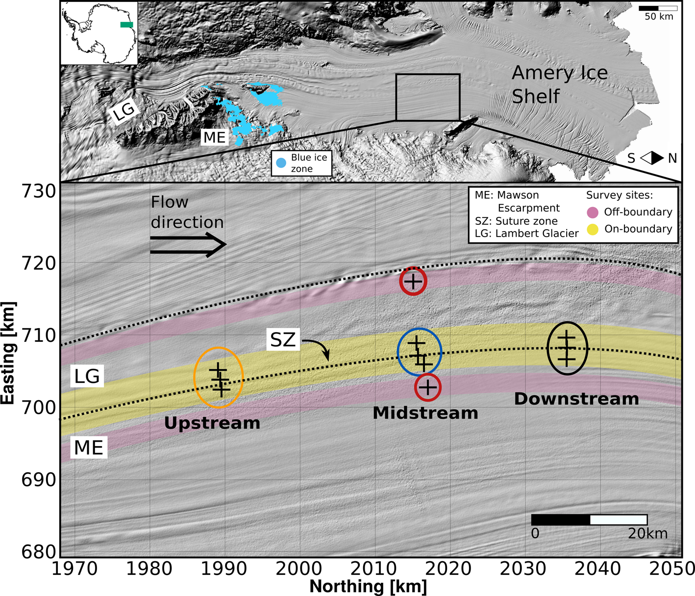
Fig. 1. Map of the Amery Ice Shelf and seismic survey region. Top: Amery Ice Shelf surface morphology, with the inset of ice shelf location. The blue ice zones upstream of the survey sites are highlighted (Hui and others, Reference Hui2014). Bottom: Details of study area. The three sample areas are highlighted by circles in orange (upstream), blue (midstream) and black (downstream); ME: Mawson Escarpment Ice Stream; SZ: suture zone; LG: Lambert Glacier, off-boundary sites (named ME East and LG West) are highlighted by circles in red; coordinates in Universal Polar Stereographic (ref. latitude: $-$ 71); approximate boundaries of relevant ice units are shown by black dashed lines. DEMs courtesy of the Polar Geospatial Center (Howat and others, Reference Howat, Porter, Smith, Noh and Morin2019).
Two additional sites, near the centre of each ice flow unit, complement the survey, where the expected simple shear strain rates are significantly lower. The survey sites were chosen using Landsat satellite images and the surface strain data of Young and Hyland (Reference Young and Hyland2002). The field team acquired two shallow seismic refraction profiles at each site, with one oriented along-flow (approximately N–S) and the other oriented across-flow (approximately E–W). Each profile comprised of a 24 channel geophone spread with groups of four 14 Hz geophones. The sources were Orica Pentex (110 g) charges, detonated along the seismic profile to provide continuous and overlapping coverage from $-480$ to $+ 480\, {\rm m}$
 offset with a variable receiver spacing averaging 5 m for offsets $\lt$
 100 m and a spacing of 10 m thereafter. The seismic dataset consists of 2.048 s records at a 4000 Hz sample rate. The along-flow and across-flow seismic profiles intersect at the centres of each profile.
We picked the first arrival travel times manually for each of the shallow seismic refraction profiles. At all sites misplacements of shot locations of up to 3 m lead to uncertainties of up to 0.45 ms. Signal to noise ratio was generally high and wavelets clearly exposed, so that the cumulative picking uncertainties are an order of magnitude smaller than the shot location misplacements. In agreement with Brisbourne and others (Reference Brisbourne2014), we therefore estimate picking uncertainty to generally be better than $\sim$ 0.5 ms.
Velocity–depth inversion from seismic travel times
We apply the 1-D velocity–depth inversion developed by Wiechert–Herglotz–Bateman (WHB) (Slichter, Reference Slichter1932) to the dataset. This approach assumes that the seismic velocity increases monotonically with depth, seismic layers are horizontally flat and the firn only varies in one dimension within a profile (lateral homogeneity on a scale of 100 s of metres). We verified the lateral homogeneity of our seismic profiles by comparing the first arrival travel times along the forward and reverse shot directions of each profile (Appendix A). The travel time differences are mostly smaller than the picking uncertainty, hence we assume each profile to be laterally homogeneous.
This allows us to apply the WHB technique to the dataset, where the seismic travel time curve of the first arrivals is a function of the seismic velocity and penetration depth of the diving waves (Slichter, Reference Slichter1932):

where $x$ is the source-to-receiver offset (in m), $u$
 the slowness at offset $x$
 with $x\leq X( u)$
 (in s m$^{-1}$
 ), $P$
 the slowness at offset $X( u)$
 (in s m$^{-1}$
 ) and $z$
 the associated depth (in m). This inversion method is employed to calculate the seismic velocity structure at the 11 sites across the Amery Ice Shelf.
The WHB inversion requires uniform sampling of the seismic slowness in the source-to-receiver offset domain. We therefore employed the exponential equation derived by Kirchner and Bentley (Reference Kirchner and Bentley1979) to produce a uniformly sampled travel time curve from the measured first arrival travel times:

where $x$ is the offset, $t$
 is the travel time and $a_i,\; \, i \in [ 1,\; \, 5] ,\;$
 are constants relating to the curvature of the travel time data. The $a_i$
 values are determined by estimating the best-fit regression to the travel time data using the trust region reflective method (More and Sorensen, Reference More and Sorensen1983). The approximation is then used to eliminate outliers from the original data before repeating the travel time approximation. Differences larger than 2 ms between the picked and the approximated travel time, presumably due to incorrect geophone placements, are considered outliers, as they imply a physically unrealistic increase in firn density. Removed data points are randomly distributed along the profiles and account for $\lt$
 1% of the data. The seismic velocities are then determined by differentiating and inverting $t( x)$
 (Eqn (3)). The associated depths were calculated using WHB method, following Eqn (1):

We performed sensitivity tests of the travel time picks to determine the impact of the picking uncertainties on the resultant seismic velocity–depth profiles. We applied the picking uncertainty to the travel time in the following ways: (1) constant offset with maximum uncertainty (positive and negative); (2) linearly increasing uncertainty (from $-0.5$ to 0.5 ms), and linearly decreasing uncertainty (from 0.5 to $-0.5$
 ms) and (3) linearly increasing (from $-0.5$
 to 0.5 ms) uncertainty for offsets $\gt$
 100 m and linearly decreasing (from 0.5 to $-0.5$
 ms) uncertainty for offsets $\gt$
 100 m. (4) Additionally, we directly accounted for the shot location misplacement by adding (or subtracting) the offset error of 3 m between 30 and 360 m, in accordance with our findings. The travel time remained unchanged for this test. The range of the resultant velocity–depth values (difference between minimum and maximum at each offset) is then used as the model error to the picking uncertainty (see Appendix B for more information).
Results
Travel times
The overall spread and the std dev. of observed first arrival travel times of each of the three sample areas (excluding the two off-boundary sites) and their related offset are shown in Figure 2a, following the colour coding of Figure 1. The near-offset travel times appear to be uniformly distributed among the survey areas and possess considerable overlap (left inset). They begin to deviate at $\sim$ 80 m offset and remain separated until maximum offset (right inset), with the upstream area possessing the smallest and the downstream area possessing the largest absolute travel times. The travel time std dev. is the largest within the upstream area with 1.7 ms and the smallest within the downstream area with 0.5 ms.

Fig. 2. (a) Spread of picked travel times vs offset for the three sample areas on the Amery Ice Shelf, off-boundary sites excluded. The minimum and maximum travel time values within each sample area are shown by lines; insets show the near- and far-offset values in more detail; the inset for far-offsets shows the average travel time and std dev. of first arrival travel times at maximum offset of each survey area. (b) Travel time differences between the along- and across-flow profiles for all of the survey sites (off-boundary sites excluded). Positive values indicate longer along-flow travel times compared to across-flow travel times, whereas negative values indicate shorter along-flow travel times compared to across-flow travel times. Thin black lines indicate the zero value. Shaded regions represent travel time uncertainty. Colour coding follows Figure 1.
The travel time differences between the along-flow and across-flow profiles of the nine survey sites near the suture zone (no off-boundary sites) are shown in Figure 2b, with the 0.5 ms travel time uncertainty shown as shaded areas. The approximated travel times (Eqn (2)) are shown for clarity. The ME and SZ flowlines exhibit travel time differences larger than the travel time uncertainty at the large offsets for the upstream and midstream areas. The travel time differences of the LG flowline remain below the picking uncertainty at all of the sample areas.
Velocity profiles
Figure 3 shows the velocity–depth profiles for all of the survey sites. The two main trends of the travel times (Fig. 2a), (i) the increase of absolute travel time, and (ii) the decrease in the range of travel times from up- to downstream, are also visible here. There are two velocity–depth profiles for each survey site, one in the along-flow direction (see inset, dashed lines) and one in the across-flow direction (solid lines). There is no separation of the travel times of the three sample areas near the surface. The separation starts at 5–10 m depth, which corresponds to 30–50 m offset. After a strong separation phase at intermediate depths of 10 to 40 m, the seismic velocities exhibit minimal overlap close to the maximum penetration depth (45–55 m depth, depending on site). At equivalent depths the seismic velocities are highest at the upstream sites, followed by the midstream and then downstream sites. The picking uncertainty of ${\pm }$ 0.5 ms converts to a maximum modelled velocity error of 2.4% (or ${\pm }$
 45 m s$^{-1}$
 ) at maximum penetration depth. The along-flow and across-flow profiles of most sites exhibit significant differences in seismic velocity, but below the conservatively chosen model error. Although the firn/ice transition zone is located at the same depth for orthogonal profiles of the same survey site, we note differences in the maximum penetration depth of up to 5 m at individual sites. The penetration depth increases by $\sim$
 8 m from 44 to 52 m along the flow direction of the Amery Ice Shelf, and the average seismic velocity at the maximum depth decreases by $\sim$
 90 m s$^{-1}$
 . The across-flow seismic velocities are generally larger than the along-flow velocities. The magnitude of both of these trends in seismic velocity is smaller than the model error of ${\pm }$
 45 m s$^{-1}$
 , but is consistent with the observed travel times (Fig. 2a).
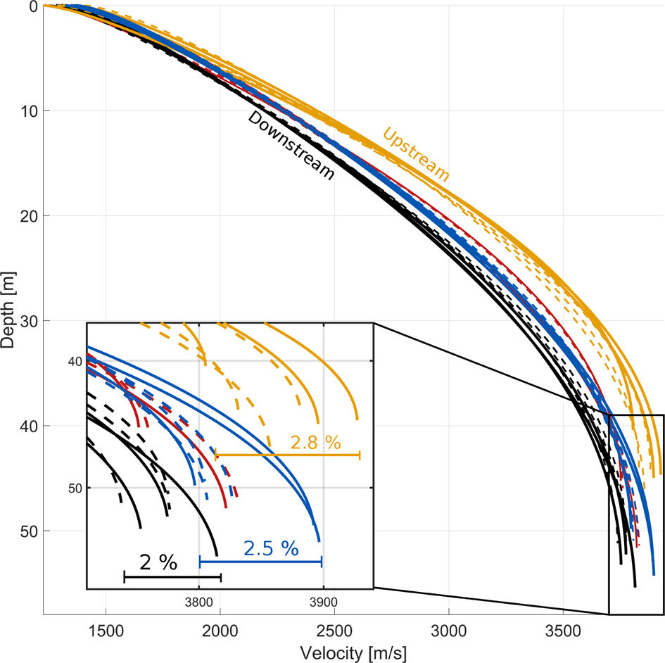
Fig. 3. Velocity–depth profiles for all of the survey sites on the Amery Ice Shelf. Each survey site is represented by two velocity–depth curves. Across-flow profiles are shown as solid lines and along-flow profiles are shown as dashed lines. The inset shows the seismic velocities at maximum depth as well as the relative range of seismic velocities of each on-boundary sample area. Colour coding follows Figure 1.
Velocity–depth values close to the firn/ice transition zone
When comparing velocity–depth values at maximum offset, which we take to be close to the firn/ice transition zone, we observe a distinct grouping according to their position along the flowline (Fig. 4). The upstream sample area exhibits the fastest seismic velocities, followed by midstream and then the downstream sample area. The upstream sample area on average exhibits the smallest penetration depths (Fig. 4), followed by midstream and then downstream with the deepest penetration depths. A comparison of the seismic velocities of the sampled flowlines with one another (Fig. 4), highlights an overlap between the survey sites on the ME and SZ flowlines, whereas the sites on the LG flowline stand out due to slower seismic velocities and, upstream and midstream, slightly shallower penetration depths (Fig. 4). The two off-boundary sites ‘ME East’ and ‘LG West’ also agree with this observation. Their velocity–depth values coincide with their corresponding flowlines, ME and LG respectively.
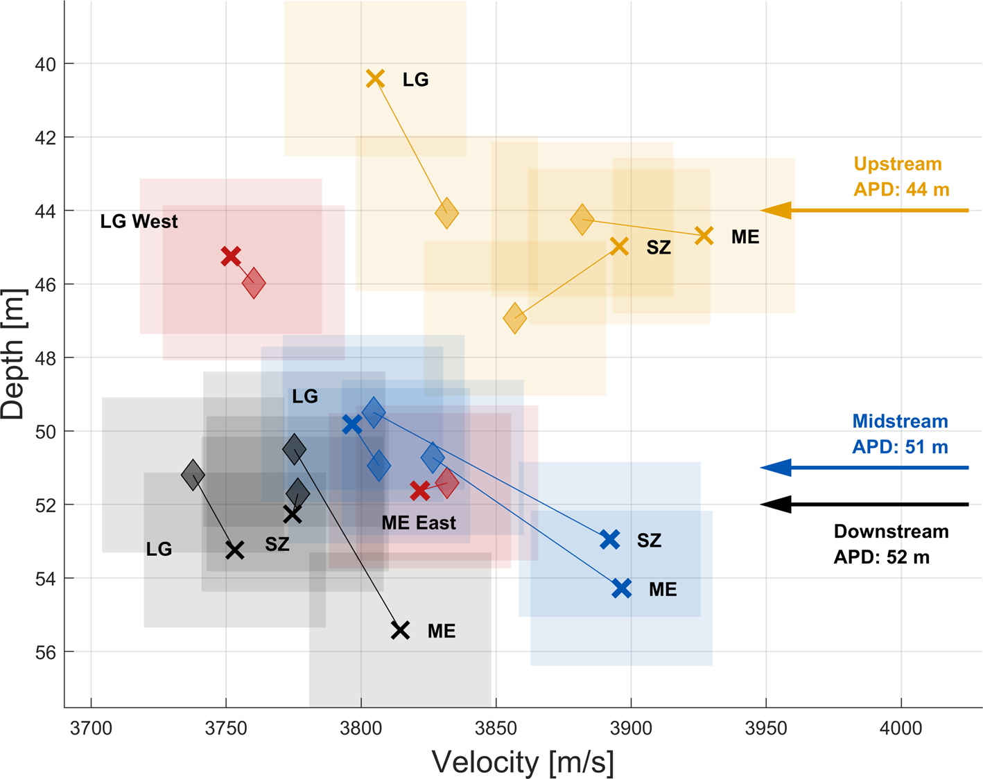
Fig. 4. Velocity–depth values of all survey sites on the Amery Ice Shelf close to the firn/ice transition zone (maximum penetration depth). For each survey site there are two values in each plot: along-flow values are marked by diamonds, across-flow values by crosses. Profiles for each site are connected with a line. The site location is displayed next to the across-boundary value of each pair (crosses). This plot should be used to compare location groups rather than single survey sites due to the significant uncertainties in seismic velocity. APD: average penetration depth of the survey area, i.e. up-, mid- or downstream. Colour coding and abbreviations follow Figure 1, with ME East: Mawson Escarpment Ice Stream off-boundary site and LG West: Lambert Glacier off-boundary site. Black circles indicate the separation of ice flow units and shaded areas show the model error.
Discussion
The seismic dataset used in this study consists of 11 individual survey sites along and across the suture zone of two major ice flow units of the Amery Ice Shelf. Sampling the ME, SZ and LG flowlines at three different locations enables the analysis of trends both parallel and orthogonal to the flow direction.
Uncertainties
The travel time uncertainty of this dataset, and with it the resulting error in modelled seismic velocity and penetration depth, is comparatively high for a seismic refraction survey, likely due to the incorrect placement of some shot locations of up to 3 m. The travel time uncertainty was chosen conservatively (i.e. high) to bolster the significance and informative value of any differences that exceed the uncertainty threshold. Differences in seismic velocity between individual survey sites are usually smaller than the model error of ${\pm }$ 45 m s$^{-1}$
 ) (see overlap of shaded areas in Fig. 4), preventing statistically meaningful comparison of differences between individual sites in this study.
However, the consistency of some trends throughout the dataset provides an insight into the characteristics of the firn. We discuss these trends here, separated into differences along and across the flow direction, to highlight the complexity of the firn structure of the region. The analysis of these trends will focus on the deep firn layer (Fig. 4), as the cause of the apparently more uniform distribution of velocity–depth values near the surface (Fig. 3) cannot be unambiguously determined in this study for two key reasons:
(1) The near-offset ($\lt$
 100 m) receiver spacing of $\sim$5 m may not adequately capture the fast densification with depth near the surface.
(2) Near the surface the firn density can vary up to $\pm$
80 kg m$^{-3}$ on scales of centimetres to metres (e.g. Freitag and others, Reference Freitag, Wilhelms and Kipfstuhl2004; Hörhold and others, Reference Hörhold, Kipfstuhl, Wilhelms, Freitag and Frenzel2011) and with it the seismic velocity by 50–90 m s$^{-1}$, for the corresponding density range (Kohnen, Reference Kohnen1972). The metre-scale vertical resolution of the seismic data is significantly larger than the thickness of most ice lenses, and the travel time approximation (Kirchner and Bentley, Reference Kirchner and Bentley1979) has an additional smoothing effect on the data. If present, high density layers would not be individually resolved and would instead result in an effective seismic anisotropy (Backus, Reference Backus1962).


We therefore focus on analysing the deeper layers, where the issues described above are of less concern. Due to lateral homogeneity of opposite shot directions for the same profile, the seismic waves of along- and across-flow profiles should travel through the same firn and, within uncertainty, yield the same velocity–depth profiles and penetration depths. We assume that the depth differences of up to 5 m for individual survey sites (Fig. 4) are caused by a combination of the model error and the seismic anisotropy of the firn. In polycrystalline ice, the seismic P-wave velocity can vary by up to 7% due to a preferred crystal orientation fabric (Bennett, Reference Bennett1968) which leads to miscalculations of the penetration depth of the same magnitude for seismic reflection surveys in polycrystalline ice (Diez and others, Reference Diez2014). For a 50 m thick ice layer this translates to penetration depth differences of up to 3.5 m. This prohibits a quantitative analysis of the velocities at maximum penetration depth of individual survey sites. Instead, the velocity–depth profiles are used to highlight differences and similarities between the three survey regions in the 2-D velocity–depth space (Fig. 4).
Along-flow trends
The average seismic travel time at the maximum offset (Fig. 1) increases from 0.145 s upstream to 0.153 s downstream. This coincides with an average decrease in seismic velocity at maximum penetration depth from 3866 m s$^{-1}$ upstream to 3771 m s$^{-1}$
 downstream (Figs 2a and 3). This decrease in seismic velocity further coincides with an overall increase in penetration depth from 44 m at the upstream sites to 52 m downstream sites (Fig. 3), or an average increase in firn thickness of 1 m per 6 km.
The firn also appears to undergo a process of homogenisation from the upstream to the downstream sample area. When comparing the travel times of profiles oriented both in the along- and across-flow directions of different survey areas with each other we note a decrease in the std dev. of travel times from 1.7 ms upstream to 0.5 ms downstream (Fig. 2 inset far offsets). This decrease is accompanied by a decrease in the range of seismic velocities from 2.8 to 2% (Fig. 3, inset). We interpret this as the physical structure of the firn becoming more homogeneous from upstream to downstream.
Across-flow trends
Aggregating survey sites along their respective flowlines (three sites per flowline) enables the identification of trends in the firn structure across the flow direction, i.e. between Mawson Escarpment Ice Stream flow unit, the suture zone and the Lambert Glacier ice flow unit. We find differences in travel times, penetration depths and seismic velocities. Firstly, the travel time differences above the uncertainty of ${\pm }$ 0.5 ms are only present on the ME and SZ flowlines (Fig. 2b). Secondly, the survey sites on the LG flowline are characterised by slower seismic velocities and slightly shallower penetration depths than the Mawson Escarpment Ice Stream and suture zone sites (Fig. 4), suggesting a separation of the firn structure along the suture zone of the two ice flow units.
The differences in penetration depth could be due to differences in the thickness of the firn, as the units originate from very different regions. Firn thickness differences across the boundary could therefore originate from a discontinuous step-like ice thickness change in the across-flow direction. This does however not explain the change in the degree of seismic anisotropy we observe to be associated with the firn thickness change, which suggests that the boundary between these two ice flow units of the eastern Amery Ice Shelf is also a boundary in the seismic structure of the firn.
Seismic anisotropy
Since seismic diving waves of orthogonal profiles at the same site sample the same firn region, the observed differences in travel time must be due to the measurement uncertainty or the directional dependence of seismic velocity in the firn, i.e. seismic anisotropy. The travel time differences for orthogonal profiles exceed the travel time uncertainty of ${\pm }$ 0.5 ms at four survey sites, i.e. the ME and SZ flowlines at the upstream and midstream sample areas (Fig. 2b). Travel time differences are caused by seismic velocity differences along the ray path. Using WHB we calculated the ray paths of the along- and across-flow profiles at these survey sites. From the travel times we conclude that at all four sites (ME upstream, ME midstream; SZ upstream, SZ midstream) the average seismic velocity is faster in the across-flow direction, as indicated by negative travel time differences in Figure 2b. This, in combination with the apparent firn thickness change that is present at the same four survey sites, suggests that the boundary between these two ice flow units of the eastern Amery Ice Shelf is also a boundary in the seismic structure of the firn. Although the velocity–depth profiles (Figs 3 and 4) could provide insight into the degree of seismic anisotropy and its development with depth, the relatively high model uncertainty of 45 m s$^{-1}$
 and penetration depth differences of up to 5 m prevent such an analysis.
The large-scale flow regime of the survey region is transverse simple shear (Young and Hyland, Reference Young and Hyland2002). Here, a combination of the direction of the compressive principal axis of the shear strain and rigid-body rotation leads to a horizontal single maximum crystal orientation fabric, oriented between 45 and $90^{\circ }$ away from the shear margin (Alley, Reference Alley1988; Budd and Jacka, Reference Budd and Jacka1989; Fujita and Mae, Reference Fujita and Mae1994).
The direction of faster seismic velocity is therefore consistent with the large-scale dynamics of the Amery Ice Shelf (Bennett, Reference Bennett1968; Diez and others, Reference Diez2014), although the two orthogonal seismic profiles per site likely do not capture the maximum degree of seismic anisotropy, as the single maximum crystal orientation fabric is likely oriented somewhere in between the two. Although the cause of this seismic anisotropy cannot be unambiguously determined on the basis of a seismic refraction study alone, the fabric that is expected along the underlying suture zone ($> \!45^{\circ }$ away from the shear margin) is consistent with the seismic findings in that the seismic velocity is faster across-flow for the LG, SZ survey sites of the upstream and midstream regions. This leaves the possibility open that the large-scale flow regime of the region plays a role in the development of the seismic anisotropy in the firn. However, if the large-scale flow regime was the dominant factor in the development of anisotropy in the firn, it should be evident at more survey sites near the suture zone, implying that other processes must be involved in the development and disappearance of seismic anisotropy in the firn.
Seismic anisotropy in the firn and its connection to the flow regime
Although there are some indications for a connection between the physical structure of the firn and the large-scale ice shelf dynamics of the region, the extent to which the flow regime of the ice masses can influence firn evolution is not clear (Salamatin and others, Reference Salamatin and Hondoh2009; Faria and others, Reference Faria, Weikusat and Azuma2014). For the deeper ice, beneath the firn, many studies demonstrate the connection between large-scale ice dynamics and the development of fabric in ice (e.g. see the reviews of Budd and Jacka, Reference Budd and Jacka1989; Hudleston, Reference Hudleston2015), but to the best of our knowledge there has not been a definitive study illustrating their influence on the intrinsic anisotropy of firn. Jordan and others (Reference Jordan, Schroeder, Elsworth and Siegfried2020) show that on Whillans Ice Stream a clear shift in the prevailing c-axis orientation is present between the near-surface layers and the deeper ice. However, in this case the deeper fabric is a result of the ice reacting to the presence of a nearby sticky spot, which limits the comparability. To investigate the possible effect of the underlying ice dynamics of the Amery Ice Shelf on the development of anisotropy in firn, we calculated the strain that could have accumulated in the firn due to the large-scale flow of the ice shelf. We base our strain estimation on Antarctica wide velocity and strain rate mosaics derived from Landsat imagery (Rignot and others, Reference Rignot, Mouginot and Scheuchl2011; Mouginot and others, Reference Mouginot, Scheuchl and Rignot2012; Fahnestock and others, Reference Fahnestock2016; Alley and others, Reference Alley2018). The presence of a major blue ice zone upstream of the study area represents a limit for where the snow accumulation of the firn sampled for this study commenced. Integrating the strain rate for each survey site along the flowline upstream to the blue ice zone provides a maximum value for the component of accumulated strain in the firn that could be due to the large-scale dynamics of the ice shelf (Phillips, Reference Phillips1998; Hui and others, Reference Hui2014). We find that the maximum accumulated strain along these flowlines is $\sim$ 0.9%, and therefore approximately an order of magnitude below that generally required for large-scale ice dynamics to produce intrinsic anisotropy in the polycrystalline ice (Treverrow and others, Reference Treverrow, Budd, Jacka and Warner2012). Laboratory studies indicate that for ice with density $\geq$
 830 kg m$^{-3}$
 , the strain required to produce a fabric in material with no pre-existing anisotropy is $\geq$
 10% (e.g. Budd and Jacka, Reference Budd and Jacka1989; Treverrow and others, Reference Treverrow, Budd, Jacka and Warner2012; Craw and others, Reference Craw, Qi, Prior, Goldsby and Kim2018). Ice core analyses demonstrate that clear anisotropic fabrics can be present close to the firn/ice transition zone (e.g. Svensson and others, Reference Svensson2003; Wang and others, Reference Wang, Kipfstuhl, Azuma, Thorsteinsson and Miller2003; Montagnat and others, Reference Montagnat2014; Treverrow and others, Reference Treverrow, Jun and Jacka2016), indicating that their development commenced within the firn at these sites.
Due to contact between firn and the underlying ice the firn must be compliant to deformation occurring in the underlying ice (Salamatin and others, Reference Salamatin and Hondoh2009). Furthermore, Faria and others (Reference Faria, Weikusat and Azuma2014) describe how densification processes within firn can produce strains high enough to generate tertiary creep over small spatial scales as the firn responds to highly localised variations in the stress field. Due to their localised nature, these deformations may not be consistent with the large-scale stress regime imposed by the ice shelf dynamics. Nevertheless, these processes provide conceptual support for the role of deformation in the development of intrinsic anisotropy within firn. In future studies, a suite of firn and snow observations would be required to identify the micro-scale processes that contribute to this anisotropy and its connection to seismic anisotropy.
Additional research is clearly required to understand firn evolution processes and reduce the ambiguity inherent to seismic refraction measurements. Where possible, we suggest that future seismic studies of firn structure should incorporate a range of complementary measurements. In addition to multi-angle seismic profiles, observations should ideally include cores that recover the firn and firn-ice transition zones, vertical strain rate information from phase-sensitive radar (e.g. Brisbourne and others, Reference Brisbourne2019) and surface GPS in order to characterise the contributions of strain and densification to firn evolution. To minimise uncertainty these measurements should be made in a zone where the upstream flow regime is both stable and consistent with conditions at the survey site. Such a study would address (i) if the seismic anisotropy present in deep firn layers originates from intrinsic anisotropy and (ii) to what extent the firn anisotropy is consistent with anisotropy present in the uppermost ice layers below the firn. In turn a better understanding of how firn evolves will contribute to reducing uncertainty in estimates of ice-sheet mass balance and the depth–age relationship in ice core climatological records.
Conclusions
We demonstrate the complex physical structure of the firn layer on the Amery Ice Shelf by analysing first arrival travel times of a seismic dataset, which reveals clear trends along and across a major ice shelf suture zone. Orthogonal profiles at each of the 11 survey sites permit the analysis of directional changes of seismic velocity (seismic anisotropy) at each site and relative seismic velocity changes between the survey sites. We observe a gradual increase of firn thickness in the downstream direction across the surveyed region. The suture zone between ice flow units appears to represent a boundary in the firn structure, with distinct firn thicknesses and average seismic velocities for each ice flow unit. At four survey sites we find travel time differences between orthogonal profiles above the picking error, which indicates a directional dependence of the average seismic velocity, i.e. seismic anisotropy, in the firn column.
Where present, the faster direction of seismic velocity does not contradict the crystal orientation fabric that is expected to be present in the underlying ice mass due to the large-scale flow regime. While this suggests that glacier dynamics may play a role in the development of firn structure, the extent to which deformation of the underlying ice mass can influence the development of the firn structure remains poorly understood. We demonstrate the feasibility of employing seismic methods to characterise the evolution of the firn in detail over large spatial scales, particularly where coring may not be feasible. However, to further understand the characteristics of firn, and to what extent this can be achieved by seismic methods, future seismic surveys should be complemented with other sampling approaches (e.g. firn coring, radar and GPS).
Acknowledgments
This research was supported under Australian Research Council's Special Research Initiative for Antarctic Gateway Partnership (Project ID SR140300001). The seismic survey was supported by the Australian Antarctic Division (AAD) ASAC Project 2581 with Richard Coleman as Chief Investigator. Data from the 2004/05 seismic survey can be found on the data portal of the Institute for Marine and Antarctic Studies, University of Tasmania (http://dx.doi.org/doi:10.25959/5e52efd1ab9e7), or via contacting the authors. We thank Alex Brisbourne, Coen Hofstede and the editor for thoughtful reviews which improved the manuscript. We also thank Christopher Watson and Richard Coleman for providing advice and assistance.
Appendix A: Travel time uncertainty
The seismic dataset contains a regular non-fixable error in the raw travel time picks. The travel times at individual offsets are in some cases separated by up to 0.8 ms. Figures 5 and 6 show the individual and merged travel time picks for the suture zone site of the upstream sample area, for both the whole offset and an enlarged middle section. The merged travel time profiles show a distinct sawtooth pattern, especially in the enlarged middle part of the profile (Fig. 6, bottom) between 30 and 360 m. Tests using synthetic data show that this pattern can be created by shifting the first arrival travel time profiles of single shot locations by 1–3 m prior to merging them to one continuous travel time profile. This indicates that the recorded location of some shots was incorrect. We account for this shot location misplacement when calculating the model error via sensitivity testing (see also Appendix B).
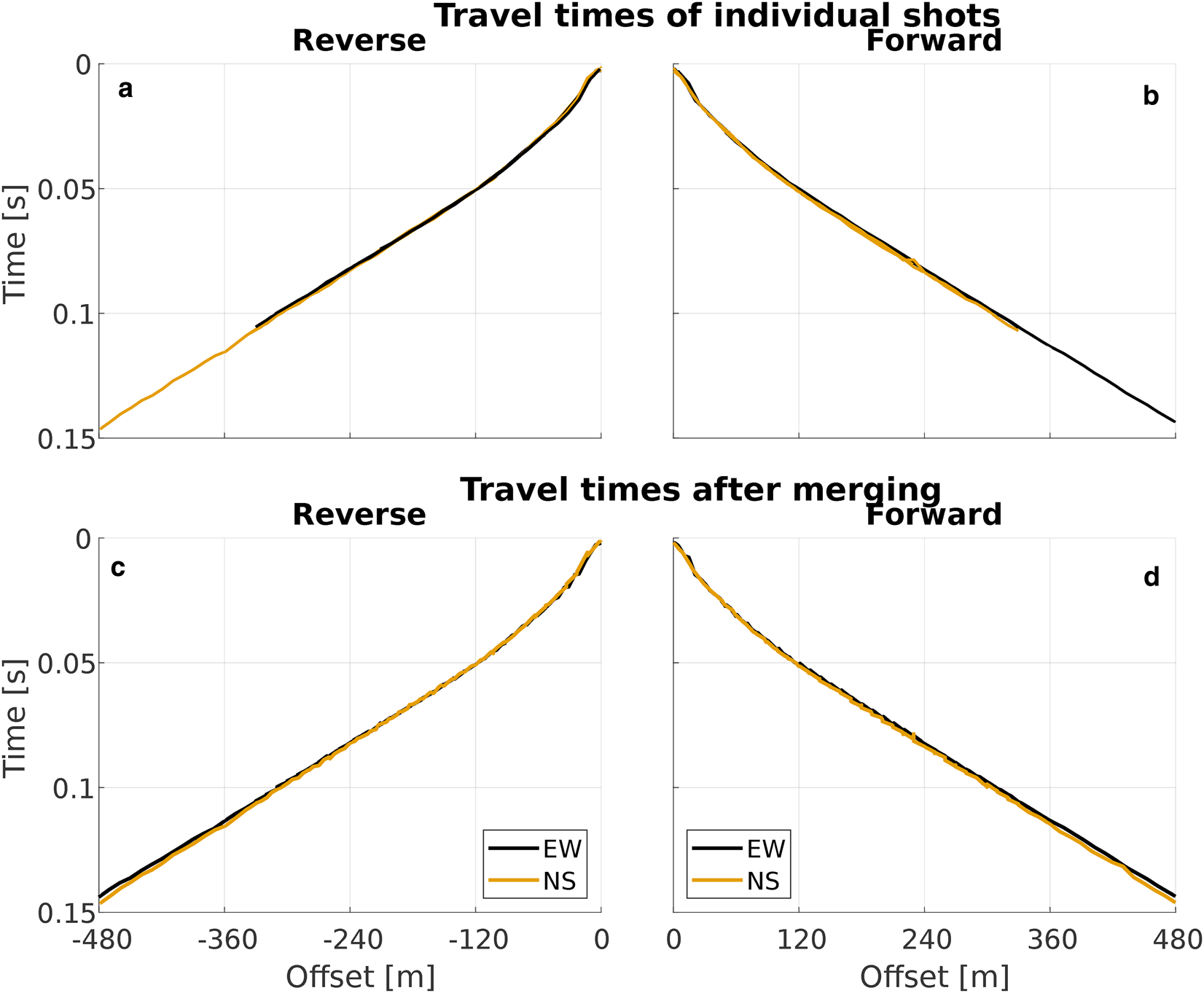
Fig. 5. Picked raw travel times of the whole upstream suture zone shot gather, separated into forward and reverse shots. (a, b) Travel times displayed in shot gathers, with each line representing one shot gather. (c, d) Shot gathers merged into their respective travel time profiles; travel times of the EW shot direction are shown in black, travel times of the NS shot direction are shown in orange (all plots).

Fig. 6. Picked raw travel times of the upstream suture zone shot gather at offsets 120–240 m, separated into forward and reverse shots. (a, b) Travel times displayed in shot gathers, with each line representing one shot gather. (c, d) Shot gathers merged into their respective travel time profiles; travel times of the EW shot direction are shown in black, travel times of the NS shot direction are shown in orange (all plots).
Appendix B: Sensitivity test and model error
In this study, the first arrival travel times were picked manually for each shallow seismic refraction profile. At all sites misplacements of shot locations of up to 3 m led to picking uncertainties of up to 0.45 ms. Signal to noise ratio was generally high and wavelets clearly exposed, so that the cumulative picking uncertainties are an order of magnitude smaller than the shot location misplacements. In agreement with Brisbourne and others (Reference Brisbourne2014) we therefore estimate picking uncertainty to generally be better than $\sim$ 0.5 ms. The consequential error in seismic velocity and penetration depth are determined by adding and subtracting the picking uncertainty to the raw picked travel times and applying the velocity–depth inversion of WHB to the new travel time profile. The picking uncertainty is applied to the picked seismic travel times in the following ways:
(1) Adding the maximum uncertainty to all data points.
(2) Subtracting the maximum uncertainty from all data points.
(3) Linearly decreasing picking uncertainty, starting at positive maximum and ending at negative maximum.
(4) Linearly increasing picking uncertainty, starting at negative maximum and ending at positive maximum.
(5) Linearly decreasing picking uncertainty at near-offset (offset $\leq$
100 m), starting at positive maximum and ending at negative maximum.(6) Linearly increasing picking uncertainty at near-offset (offset $\leq$
100 m), starting at negative maximum and ending at positive maximum.(7) Adding 3 m to one data point of the offset every 10 m to imitate the shot location misplacement. We limited it to offsets between 30 and 360 m in accordance with our findings. About 40% of the data were changed and the travel time was not altered for this test.
(8) Subtracting 3 m to one data point of the offset every 10 m to imitate the shot location misplacement. We limited it to offsets between 30 and 360 m in accordance with our findings. About 40% of the data were changed and the travel time was not altered for this test.


Next, the difference between the maximum and minimum values of penetration depth and seismic velocity of all nine velocity–depth profiles (including the original profile) was determined for every offset. The result was a single profile for penetration depth and seismic velocity that we used as a measure of the model error (Fig. 7). The model error, especially at large offsets, is considerably larger than what can be found in other studies (Kirchner and Bentley, Reference Kirchner and Bentley1979). This is mainly due to the shot location misplacements, as described in Appendix A (Figs 5 and 6).
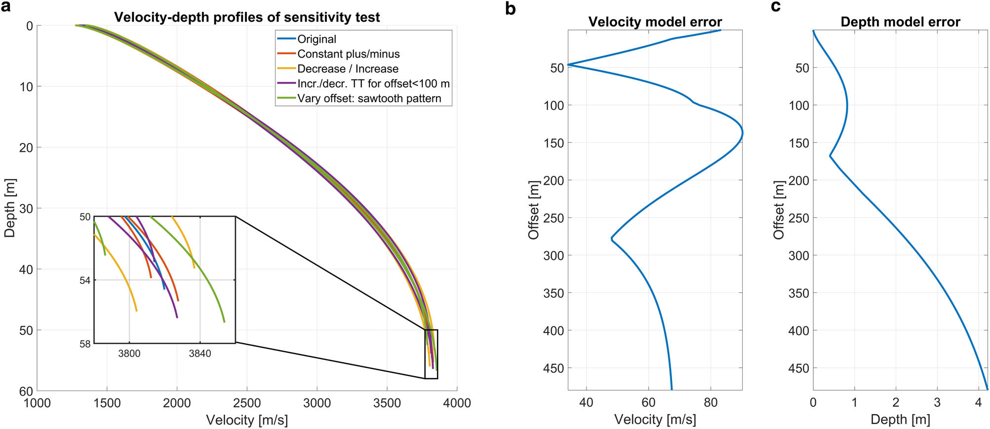
Fig. 7. Error in seismic velocity and penetration depth assuming a ${\pm }$ 0.5 ms picking uncertainty. (a) Velocity–depth profiles after applying the picking uncertainty to the travel times in different ways (see legend). (b) Range of the velocity error versus offset. (c) Range of the depth error against offset.


 Open access